
Quantifying Geodiversity at the Continental Scale: Limitations and Prospects

Institute of Geology, Adam Mickiewicz University, Bogumiła Krygowskiego 12, 61-680 Poznań, Poland
Resources 2023, 12(5), 59; https://doi.org/10.3390/resources12050059
Submission received: 31 March 2023
/
Revised: 11 May 2023
/
Accepted: 12 May 2023
/
Published: 17 May 2023
(This article belongs to the Special Issue Geodiversity Assessment: What, Why and How?)
Abstract
:Geodiversity, defined as the natural range of geological, geomorphological, hydrological, and soil features, has been explored in a growing number of studies at different spatial scales. However, most research efforts have been directed at analysing geodiversity at a fine-scale. Here, an estimation of the geodiversity of the European subcontinent is performed using six available high-resolution global data sets that describe the diversity of selected features of the abiotic environment. Six maps representing geomorphological, geological, hydrological, hydrogeological, soil, and topographical diversity are compiled using the methods of centroid analysis and kernel density estimation. The present contribution identifies areas with high values of most geodiversity variables which were not previously studied, nor are included in the network of international geoparks. The study also shows that, although remote sensing images and digital elevation models allow one to grasp a significant understanding of geodiversity on the continental scale, fine-resolution and process-oriented geological data sets are required to further enhance the quality of large-scale geodiversity assessments. To ensure interoperability between studies, a consensus is necessary regarding the analytical methods, classification rules, standardised indices and dictionaries. Without this, comparisons of geodiversity evaluations across different scales and between distant study areas remain difficult.

1. Introduction
Although the importance of abiotic natural resources considered as natural features and assets that foster the diversity of living organisms (i.e., biodiversity) and sustain the human economy is widely accepted, it has only been in recent years that their evaluation has received attention and become the subject of study. From the beginning of the 1990s, and the introduction of the term “geodiversity” (which broadly refers to the diversity of abiotic nature [1]), research related to the assessment of the natural range of nonliving components of the lithosphere, hydrosphere, abiotic products of the biosphere and, in some cases, the atmosphere, became a central theme of a growing number of scientific papers. This was followed by recognition of the importance of geodiversity evaluation to conserve biodiversity [2], for tourism development [3] and for the future of sustainable economies [4]. This has led to the conclusion that the strict definition of geodiversity and its careful evaluation are important for the rapidly expanding global economy and for the preservation of natural diversity, both biotic and abiotic, for future generations [5,6].
Despite the growing number of studies, a unified definition of the term geodiversity has not yet been adopted by all scholars active in the field. The most widely accepted view is that geodiversity encompasses a range of geological, geomorphological, hydrological, and soil characteristics, following the concept of Gray [7]. Competing opinions, supported by a smaller number of published contributions [8], are broader, and include ex situ geological features such as building stones [9], nonrenewable energy resources [2], and climate diversity [10]. Conflicting views on geodiversity are accompanied by a lack of universal classifications of geodiversity elements [11] and the multitude of available evaluation methods [12]. These specific features of geodiversity research limit the interoperability of individual studies.
Geodiversity estimations and their relationships with biodiversity are scale dependent [13]. The aim of the research usually defines its scale; studies that explore the abiotic diversity of habitats and micro-habitats necessarily operate on a scale of individual plots [14], while investigations of tourist potential requires assessments over large areas or on numerous sites of geological interest [15]. Geodiversity elements also differ in scale, from individual outcrops of various rock types to huge landforms and large groundwater reservoirs. This involves further difficulties when comparing the results of research that refer to different scales and discordant lists of geodiversity elements.
Although the amount of geodiversity research grows exponentially [16], relatively few studies explore abiotic diversity on multinational, subcontinental, continental [17,18], or global scales [19]. This makes existing studies at the medium and small scales more dispersed. It also reduces the interoperability of the evaluation methods and impedes the introduction of standardised classification methods that could be used at broader scales of regions and continents. The apparent scarcity of large-scale empirical studies also results from the limited availability of spatial data that cover large areas or, better still, the entire world. However, in recent years, the advent of satellite remote sensing and geographic information systems has resulted in global data sets containing geodiversity variables [13]. This facilitates geodiversity assessments over large areas and comparisons with local studies. Regional- and continental-scale geodiversity estimations are also important due to the scale dependence of some geodiversity elements. Therefore, studies across scales can reveal patterns that would otherwise remain hidden, similar to the procedures involved in biodiversity research [20].
This study aims to quantify geodiversity on a continental scale and identify regions with a diverse set of abiotic resources, that is, high geodiversity. Similar to biodiversity hotspots, such areas are termed geodiversity hotspots when they undergo significant anthropogenic pressure [21]. The identification of such areas is important for future conservation efforts [22] and for tourist development. Another goal of the study is to compare the outcome of the geodiversity evaluation with the results obtained in earlier small-scale studies conducted within the same area and with the use of different methods and geodiversity elements, to estimate the impact of the absence of widely accepted standards and methodologies. We hypothesise that the use of different scales, from continental to mesoscale, will reveal geodiversity patterns not detected when using a fixed spatial level in the analysis. Comparison of geodiversity evaluations at the continental scale with earlier research efforts will also permit the location of geodiverse areas that have not yet been studied or assessed for relevance in current areas of natural protection networks; their tourist potential has not yet been adequately recognised. The area of study covers Europe, which has been extensively investigated in terms of geodiversity and the tourist potential of regions with significant abiotic diversity, but most studies have been performed at finer scales.
2. Materials and Methods
2.1. Study Area
The study area included the entire European subcontinent (Figure 1), ranging from Iceland and the Azores in the west to the Ural Mountains in the east, and covering an area of approximately 10 million square kilometres. The choice of study area is justified by a significant number of earlier studies that assessed geodiversity at micro to mesoscales. When considering the number of published research contributions in 2019, Europe outnumbered all other continent by at least three times [16]. Furthermore, more than 50% of UNESCO world geoparks are located in Europe. Therefore, the use of the European subcontinent as an area of study facilitates comparisons with earlier studies at smaller scales and allows estimation as to whether areas with high scores of geodiversity and numerous geodiversity elements are represented adequately in current research. This permits the identification of possible gaps and biases, suggesting possible future directions of study.
2.2. Geodiversity Elements and Data Sources
Geodiversity is the natural range of geological, geomorphological, hydrological, and pedological features, including their contribution to the landscapes [7], although other definitions are also used [8]. The choice of the concept of geodiversity determines the list of geodiversity elements that are studied. Some approaches include the climatic diversity within the geodiversity [23]. Other frameworks introduce abiotic diversity (defined as the union of climate diversity and geodiversity [24]) and establish a separate entity, termed climatediversity [25], to complement existing concepts of biodiversity and geodiversity. In this work, climatic diversity is excluded from geodiversity because it is not included in the widely accepted definition of geodiversity. Therefore, the list of geodiversity components used in the present study includes six items (Table 1), which are discussed in detail below. For each geodiversity element, one variable that best reflects the state of this feature was selected for this study. Only global data sets were used for each variable to allow future for comparisons among other continents.
2.2.1. Geomorphodiversity
The diversity of landforms is included in the widely used definition of geodiversity [7]. In some studies, the geomorphological component of environmental diversity is termed geomorphological diversity [34] or geomorphodiversity [35,36], but its affiliation with geodiversity is not questioned [36]. Research on landform diversity at a large scale is hampered by limited data availability [37], as there are no detailed geomorphological maps on a global scale. However, metrics related to the landscape heterogeneity can be extracted from standard digital elevation models (DEMs). Here, the concept of geomorphons (scale-dependent, elementary units of terrain [38]) was employed. The package r.geomorphon [27], available within the QGIS environment, was used to obtain landform data from the global digital elevation model MERIT DEM [26], which offers an angular resolution of three seconds (approximately 90 m at the equator). Geomorphons were extracted using default parameters of outer search radius (3.0) and flatness threshold (1.0), which determined the scale of the landform features and the angle at which the ground was considered flat, respectively.
Although the use of geomorphons allowed for the mapping of ten of the most common standard landform types, it returned no indications regarding their origin. Furthermore, the morphological characteristics of the ice covers are not analysed independently of the features of the ground surface. On the other hand, the introduction of the classification of the geomorphological features into genetic classes has proved to be a valuable tool In assessing geodiversity, particularly at its intersection with biodiversity [14]. Thus, geodiversity studies would benefit from new continent-scale geomorphological data sets. This would also give more insight into the processes that shape landscapes; these are also included in the definition of geodiversity [7]. Thomas [39] has stressed the importance of the processes and events that influence geomorphodiversity.
2.2.2. Hydrodiversity
Hydrological diversity, or hydrodiversity [21], is defined as the diversity of the surface water resources of the Earth and is included in the prevailing geodiversity concepts [6,7], considered an integral part of geodiversity in many studies [40,41,42,43]. Other frameworks place hydrodiversity in a broader category of environmental heterogeneity [44]. In the present study, hydrological resources were included in geodiversity estimation, and their diversity was assessed using the Global Water Body Map data set, developed using an automated algorithm to analyse multitemporal Landsat images, having an angular resolution of three seconds [28]. The data source contains the spatial extents of permanent water, temporary flooded areas, salt marshes, wet soil, and snow cover.
2.2.3. Hydrogeological Diversity
Although hydrogeological resources were not explicitly indicated in the definition of geodiversity followed in this study [7] but were incorporated into a broader category of hydrological features, and underground water resources were determined using the subsurface geology [45], which constitutes an integral part of geodiversity. To quantify the diversity of groundwater resources, the depth of the groundwater table, retrieved from the Fan et al. [29] data set, was used as a parameter. Variability in the level of the groundwater table is considered to have an impact on vegetation cover [46] and the heterogeneity of native habitats. The data source used in the present study was compiled using observations of the water table from wells and a groundwater model forced by climate and topography [29]. Well data are not uniformly distributed, with significant gaps (e.g., in the eastern part of the European subcontinent). Although the model is global, no data were available for most of Iceland’s territory.
2.2.4. Lithological Diversity
The diversity of geological resources (rocks, minerals, mineral deposits, fossils) is among the most frequently used components of geodiversity [6]. In the present study, two global lithological data sets were used: (1) Global Lithological Map (GLiM) [30] and (2) Global Unconsolidated Sediments Map Database (GUM) [31]. The average resolution of both maps was approximately 1:3,000,000, significantly less than in the case of the other data sources featured in the present study. The GLiM database does not include information on unconsolidated sediments, instead using the lithological units located beneath [30]. Therefore, the data retrieved from the GUM database were also used for the purpose of the present study. Both data sources were compiled from maps provided by national geological services; due to the heterogeneity of the data sources (that is, the names of lithological types), a classification was applied to the data set [31]. From the GUM database, the sediment type variable was used in the present study, while codes of dominant lithologies were recovered from the GLiM map.
Other metrics of lithological diversity not used in the present study include mineralogy [43], fossil content [47,48], and superficial deposit richness [37]. They are less common in existing quantitative assessments of geodiversity [6], although mentioned in the classic definition [7]. They were not used in the present study because there are currently no global maps for these features. In the future, it should be possible to use data from the Mindat.org and the GEMI databases for mineral occurrences [49], and from the Palaeobiology Database (PBDB) [50] for the locations of fossils.
Geodiversity characteristics related to geophysical processes, such as land subsidence, earthquakes, volcanic eruptions, and surface materials dynamics, were not used in the present study, although their inclusion within the geodiversity assessment frameworks was postulated [2]. Although there are data sets available for some of these variables (e.g., seismological data) and others can be measured from existing remote sensing data using automated algorithms (e.g., subsidence patterns retrieved from Sentinel satellite images [51]), most of the information regarding the geological processes that underlie lithological variation on the Earth’s surface is difficult to estimate using machine learning and requires careful interpretation. Thus, although the analyses of such geodiversity features, included in the tentative list of Essential Geodiversity Variables (EGVs) compiled by Schrodt et al. [2], will involve extensive research efforts, and it would give additional information on environmental diversity.
2.2.5. Pedodiversity
Pedodiversity studies aim at describing the diversity of soil types in a given area [11] and determining the variation in standard soil properties. Although considered part of geodiversity [13], pedodiversity research has traditions which are longer than, or at least comparable to, investigations of geodiversity [11]. This resulted in the adoption of mature standards and classification schemas, which allowed the compilation of high-resolution global databases of soil types and numeric soil properties. In the present study, the SoilGrids250m database [32] was used. Soil classes coded using the international World Reference Base classification system were employed as a parameter for pedodiversity quantification. The data set includes predictions based on soil profiles and soil covariates from remote sensing [32].
2.2.6. Topographic Diversity
Although topographic heterogeneity is included in the widely accepted definition of geodiversity [7], its status differs significantly among individual studies. Many frameworks aimed at geodiversity evaluation feature topographical variables [13,17], while others replace them with metrics of landform diversity [2,52], exclude topography from geodiversity elements and assess it separately [42,43], or move it into a wider category of environmental heterogeneity [44]. Among the topographical measures, elevation (i.e., mean and standard deviation), slope angle, and orientation of a slope (i.e., aspect), topographical wetness index, and terrain ruggedness index are some of the most widely used [37,53]. The number and wide use of these features is, in part, due to the ease of obtaining the data. All topographic variables can be calculated from the DEM. The abundance of topographic diversity metrics imposes their careful choice and use. Basic features such as elevation, slope angle, and aspect are frequently analysed simultaneously. However, although these variables are found to provide important information, their strong collinearity lowers the general usefulness of their application [37]. On the other hand, the terrain ruggedness index (TRI) receives recognition as a valuable metric of terrain heterogeneity and its potential use in geodiversity studies at different scales has been explored in detail, [53]. Although not deprived of certain limitations, such as dependence on altitude and differences in elevation, TRI is a reasonable choice for a single metric that describes topographic heterogeneity and, therefore, was used in the present study. The feature was calculated from the MERIT DEM world digital elevation model [26], following the algorithm by Riley et al. [33].
2.3. Geodiversity Assessment
The selection of methods used for the evaluation of geodiversity is among the most difficult challenges in geodiversity studies, regardless of their scale [12]. This results from the multitude of assessment methodologies and statistical procedures employed in previous research in this field [6]. In a review of the existing methods, Zwoliński et al. [12] divided available assessment frameworks into (a) direct and indirect and (b) qualitative, quantitative, and qualitative–quantitative. Indirect methods do not require fieldwork, as geodiversity attributes are calculated from existing data sources within a geographic information system (GIS) environment. Therefore, they were used in the present study, allowing geodiversity evaluations to be performed on large areas.
Quantitative methods of geodiversity estimation are used the most frequently [12]. Therefore, they were considered to be the most suitable for the purpose of this contribution, which covers a large study area and aims to compare the results with previous research efforts. Parameters that numerically describe geodiversity are employed as input for quantitative methods, whereas indices and map algebra are used to estimate the intensity (diversity) of multiple geodiversity features [54]. Although the geodiversity index [5,55,56] has a long history and has been used in numerous studies, its formula is still disputed by the scientific community and undergoes modifications. The use of one combined variable is also unfavourable in many geodiversity studies, particularly those exploring the intersection of abiotic and biotic diversity [37]. Moreover, indices operate on spatial units of different shapes and areas, by forming a grid over the study area in most cases [6]. The resolution of the grid is taken at the beginning of the analysis. However, in the present study, it was difficult to judge the best possible type and dimensions of the grid due to the use of diverse data sources, which were available in raster formats. This means that these data sources were, in fact, gridded with resolutions that are not the same in all data sets. Moreover, it is not possible to use a single grid dimension when comparing the results of the evaluation on multiple scales. Thus, the approach that involves the use of spatial analytical tools and map algebra was better suited for the purpose of the present study than the use of a geodiversity index.
To avoid the drawbacks of grid-based geodiversity evaluation, the centroid analysis method [52] followed by kernel density estimation [1] was used to count geodiversity elements within the study area. Centroid analysis involves finding the geometric centres (centroids) of polygons that represent the spatial extent of a geodiversity element, or an area exhibiting the same or comparable values of a geodiversity variable. Kernel density estimation was used to visualise the spatial density of centroids for a given variable [57], allowing us to create maps showing hotspots and coldspots representing the expected number of centroids per unit area. The resolution of the maps obtained was determined at the end of the workflow, which is a more robust solution, enabling easy testing across scales, and this is essential for comparing the study outcome with earlier contributions at mesoscale and microscale. No statistical modelling was used to simplify the assessment procedure. The choice of available statistical tools is usually determined by the purpose of the study, and their use is most common in research that explores the links between geodiversity and biodiversity [2]. The outcome of the present contribution does not include conclusions regarding the relationship between the biotic and abiotic diversity, because geodiversity poorly improves biodiversity models at large scales [37]. Thus, statistical modelling was not included in the study design. A detailed outline of the geodiversity assessment framework used in this study is provided below and shown in Figure 2. The resulting maps are shown in Figure 3 and Figure 4 and Supplementary Materials S1. Correlation matrix among the geodiversity variables is included in Table 2. For all spatial analyses, the QGIS software was used.
2.3.1. Data Preprocessing
All data sets used in the present study were global in scale. The first stage of data preparation was, therefore, to crop the layers to the extent of the study area (i.e., to the European subcontinent). Clipped data sets were reprojected into the WGS 1984 coordinate referencing system when necessary. Some of the geodiversity variables chosen for the purpose of this study need to be calculated from existing global data sources. Therefore, the second step of the analysis was to detect geomorphons and calculate the TRI values from the DEM. During the next stage of data preparation, the raster layers containing values of water table depth and TRI were reclassified based on ranges provided in the Figure 2 to enable the use of continuous data in the subsequent conversion to the vector format.
In the fourth step, a sieve filter was applied to the raster data. The filter removed elements whose surface areas were smaller than the chosen number of pixels (eight in this study) and pixels that were not adjacent to any other pixel sharing the same value (the connectivity of eight), replacing them with pixels representing the surrounding objects [58]. This step was employed to reduce the computation time and facilitate the analysis of a large area.
Both the centroid analysis and kernel density estimation, used in the present study, require the data set to be in vector format. During the final stage of data preparation, the resulting raster layers were converted into polygonal (i.e., vector) layers and reprojected to the LAEA-ETRS89 projection.
2.3.2. Centroid Analysis and Spatial Smoothing
The main phase of the analysis included the process of locating centroids of polygons on vector layers and the spatial aggregation of data to obtain density maps using kernel density estimation. The centroid localisation algorithm returned vector point layers, which served as inputs to the kernel density function. The kernel density estimation recovered the underlying structures of data sources [59], resulting in the generation of a raster map that represents the number of centroids in a given unit area [52]. Although no grid is imposed on the data sets when kernel density estimation is employed [1], the value of the radius parameter, which defines the distance at which neighbouring points are counted, was selected at this stage of the analysis. The resolution of the source maps [52] and the experiments [1] were used in previous studies, to determine the most suitable radius value. The same approach was adopted in the present study, although more objective methods of optimal radius selection can be employed in the future [60]. The cell size defines the resolution of the resulting map. Two sets of maps were generated by applying the following values of the radius and cell size parameters:
- High-resolution maps included in Supplementary Materials S1 (radius of 5 km and cell size set to 1 km to ensure a high resolution of the resulting maps).
To generate a final map showing the diversity of all characteristics of the geodiversity and representing the total expression of the geodiversity, map algebra functions were employed [12]. Each raster map obtained as an output from the kernel density estimation was normalised between 0 and 100. Missing data values were replaced by zeros, to enable calculations on raster pixel values. The arithmetic mean of all raster layers was then calculated and clipped to the study area, resulting in a final map that visualised the total geodiversity, allowing one to locate possible geodiversity hotspots. No weights were applied to geodiversity elements, although recent studies show that there is a possibility of weighting geodiversity features by multivariate statistical analyses [56].
During the last stage of the analysis, the geodiversity variables used in the present study were tested for possible correlations. This particularly applies to features that were derived from the same source (geomorphons and TRI values, both obtained from the DEM). A covariance matrix for the raster maps obtained by smoothing the kernel was calculated using the r.covar function (Table 2).
2.4. Review of the Literature
Systematic reviews of the literature provide an overview of the current state of research, finding research gaps, and locating areas of uncertainty [61]. Here, a bibliographic review was used to identify earlier contributions that aimed at analysing microscale- and mesoscale geodiversity of study areas located in Europe. We hypothesised that the intensity of research reflects the location of geodiversity hotspots identified in the present study. The literature review can also be used to recognise areas that show high geodiversity but are not investigated enough and can be used as study areas in the future.
The bibliometric analysis procedure was based on three steps:
- Literature search;
- Selection of relevant papers;
- Data extraction and analysis of results.
The method used in this study is summarised in Figure 5.
During the first stage, the Scopus and Web of Science databases were used. The search strings used to retrieve relevant papers are listed in the Figure 5. The term “geoheritage” was also included in the queries. Although the geodiversity and geoheritage assessment are considered to be separate research areas [6,62], the term geoheritage is frequently, but incorrectly, used as a synonym for geodiversity. Geoheritage is defined as the part of geodiversity essential for reconstructing the history of the Earth [7] or as in-situ and ex-situ geodiversity elements with high scientific values [62]. Apart from its importance for the scientific community, some authors use a broader definition of geoheritage, including geodiversity elements that exhibit outstanding educational and/or cultural values [63]. Despite the differences between definitions, it is clear that high levels of geodiversity do not necessarily correlate with geoheritage because elements of geodiversity which are important from a scientific point of view can appear in areas of low abiotic diversity.
The research was carried out in January 2023. The literature search returned a total of 794 results from the Scopus database and 614 results from Web of Science. In the subsequent step of the analysis (step 2 in Figure 5), the duplicate records were removed from the results. The outcome of this stage included 1108 items. The abstracts were screened to identify publications that are not directly related to the theme of geodiversity and/or geoheritage assessment. Studies that do not involve specific study areas or investigate ex-situ geodiversity elements, such as building stones, were removed from the database, reducing the volume of data to 202 items. In the last step of the literature review (step 3 in Figure 5), the geographic location of each contribution was determined and mapped (Figure 6 and Figure 7). The most prominent themes of each contribution were identified by analysing the title and key words of the papers (noting that some papers explore several topics in similar depth). As a result, an Excel datasheet was produced with bibliographic data and the information obtained from the text (Supplementary Materials S2).
The scientific reports that have not undergone peer review were not included in this review of the literature. Therefore, the total amount of labour for the documentation and promotion of geodiversity of the European continent was larger than that evaluated in the present contribution, but the application of scientific databases allowed for a satisfactory approximation of recent efforts and the identification of current research trends related to geodiversity evaluation.
2.5. International Geoparks
UNESCO Global Geoparks (UGGs) are territories of international relevance whose geodiversity characteristics allow visitors to appreciate and experience geological and geomorphological features, and their sustainable development is supported by the local community [64]. The network of UGG includes (in January 2023) 177 members in 46 countries. The European Geoparks Network (EGN) aims to improve the recognition, conservation, and promotion of geoheritage [65]. In January 2023, it unites 94 geoparks from 28 countries. This number does not include local geoparks introduced at the national or local administrative levels.
The exceptionality of geological features regarded as an aspect of geodiversity of these at the heart of the geopark concept, although it also integrates elements of biodiversity and cultural heritage [66]. Geoparks are established as a means of efficient conservation of unique geodiversity elements [67]. High scores are obtained from the evaluation of the geodiversity resources of selected existing global geoparks [68]. However, the presence of an UGG or EGN member does not necessarily indicate high geodiversity in the area because the geological heritage of international relevance is not correlated with high levels of geodiversity. The amount of conservation efforts can also be independent of the results of geodiversity evaluation. Furthermore, the presence and number of UGG and EGN members does not reflect a complete coverage of the studies related to geodiversity and geoheritage, because some countries have not yet adopted the concept of international geopark networks but use national geoparks and natural reserves instead. In addition, the designation of a new UGG and EGN member requires substantial input from local communities, regardless of the scientific efforts to assess geodiversity and identify geoheritage sites in the study area. However, the locations of the international geoparks were used as a useful approximation of the recognition and appreciation of the geological heritage and as a means of identifying areas that show a distinct and very diverse set of geodiversity characteristics and resources, for which no global or European geoparks have yet been established, suggesting possibilities for future development.
The geographic coordinates of current UGG and EGN members were recovered and used (after removing duplicates) to map geoparks located in the study area (Figure 6). As a result, a list of 90 geoparks located within the study area was compiled (Supplementary Materials S3).
2.6. Case Study
To bridge the results obtained for the whole of the European subcontinent with earlier research efforts at mesoscale- and microscale, a case study was performed on a national scale, using the territory of Poland, which covers an area of approximately 312,000 square kilometres. The selection of a state for this step of the analysis was based on the amount of earlier research efforts and the number of published contributions that provide detailed maps of geodiversity. Poland is among the countries with the highest number of geodiversity and geoheritage studies [16], and a review of the literature revealed several articles that included estimates of geodiversity and detailed geodiversity maps at a local scale (Supplementary Materials S2). This shows the rationality of using Poland as a study case.
Six earlier geodiversity studies from selected areas of Poland were used to test the results obtained using the current methodology [15,69,70,71,72,73]. Contributions that refer to study areas covered by subsequent studies [74], or only evaluate topographical or geomorphological diversity [75,76], were excluded from this comparison. From each of the previous studies selected for comparative analysis, the boundaries of the study area and the areas that exhibit the highest values of total geodiversity (geodiversity class termed “very high”) were extracted and mapped on the base map of compound geodiversity, which was obtained in this study (Figure 8).
Geodiversity maps allow local policy makers and managers to include future geoconservation efforts on regions that reveal the highest scores of total geodiversity during centroid analysis and, therefore, host the richest assemblage of abiotic resources. To determine whether existing protected areas established on the territory of Poland are associated with the extent of enclaves of high geodiversity values, the boundaries of protected areas were plotted on the base map of the total geodiversity, as estimated in the present contribution (Figure 9). The following types of protected areas were established in Poland, including national parks, landscape parks, Nature 2000 network, protected landscape areas, and nature–landscape complexes. Nature reserves and natural monuments were excluded because the study of their distribution requires finer scales of geodiversity maps. The purpose of many protected areas is to facilitate the conservation of biodiversity; therefore, their distribution cannot be directly compared with the locations of geodiversity hotspots. However, they were used to identify areas with significant abiotic resources that are not yet included in the national network of protected areas.
3. Results
3.1. Geodiversity Evaluation
The geomorphological diversity of Europe, analysed using the geomorphon concept, revealed high values for most of the continent (Figure 3a), partly reflecting the high resolution of the source DEM and the low radius parameter of the r.geomorphon algorithm [27]. The lowest number of geomorphons per unit area was obtained for lowlands and alluvial plains (the Caspian Depression, Po Plain, Romanian Plain, parts of Pannonian Plain, and Polesian Lowland). The highest values were recorded for mountainous areas (the Carpathians, Apennines, Dinarides, Scandinavian Mountains, Alps, Cantabrian Range) and for highlands (Massif Central, Central German Uplands, Southern Swedish Uplands). Absolute or relative heights do not determine geomorphodiversity, as shown by the high values obtained for the Timan Ridge and Northern Uvaly, in Russia.
Hydrological diversity (the number of hydrological features per unit area) reveals lower and less differentiated values (Figure 3b). The highest numbers are obtained at the northern margin of the subcontinent (Iceland, Svalbard, the environs of Lake Inari, the northern coast of the Kola Peninsula, Novaya Zemlya, and the lower course of the Pechora river), with smaller enclaves located in southwestern Norway and along the lower course of the Volga river. The interior and southern parts of the European continent exhibit low and relatively undifferentiated values of hydrological diversity.
The diversity of the underground water table levels shows another pattern. Peak values are noted in Norway (Figure 3c), in the highest and most extensive mountain ranges (the Alps, Caucasus, Dinarides, Pyrenees), in Svalbard, and, to a lesser extent, in the northern peripheries of the continent.
The map of lithological diversity (number of outcrops of lithological types per unit area) reveals a significant bias caused by unequal sampling (Figure 3d). Most countries in the European Union and Great Britain show more prominent lithological variation compared to the southeastern part of the subcontinent and Russia. Peak values are recorded for Ireland, Belgium, and Denmark, followed by Germany and Switzerland. The estimated lithological diversity changes sharply at many administrative borders, showing that both GLiM and GUM databases are compiled from heterogeneous sources that differ significantly in resolution, artificially lowering the geological diversity of southeast and eastern Europe.
Soil diversity shows high and variable numbers of World Reference Base classes throughout the continent; its patterns differ from those noted for other maps (Figure 3e). The highest values are obtained for Poland, northern Germany, Lithuania, Latvia, and the northern Ostrobothnia of Finland. The lowest diversity is recorded for the East European Plain, north of the Central Russian Uplands and south of the Timan Ridge.
Topographic diversity is defined as the number of centroids of areas with comparable values of TRI (after reclassification), calculated per unit area, which is highest in mountainous areas, notably the Alps and the Caucasus and, to a lesser extent, the Pyrenees and the Dinarides (Figure 3f). Increased values have also been obtained for Svalbard. The lower mountain ranges and highlands show relatively low values of TRI, similar to those obtained for the lowlands.
The composite map of geodiversity (Figure 4) allows for the identification of areas that show high values of most geodiversity metrics. On the European subcontinent, such areas are mapped in the eastern fringe of the Western Alps, in the vicinity of the Sognefjord in Norway, on the Barents Sea coasts (west from Murmansk and in the vicinity of the Haypudyrskaya Bay of the Pechora Sea), in Nordaustlandet in the archipelago of Svalbard and in the Caucasus. The fine-resolution map supports these findings (Supplementary Materials S1). High values are also noted in Ireland and Denmark, but these are the result of high values of lithological diversity as a result of oversampling. The lowest values are found for the plains (the Netherlands, the Caspian Depression, the Pannonian Plain, the Po Plain, the Polesian Lowlands, and the Romanian Plain). The largest lakes in Europe are also marked with low values of geodiversity because most variables cannot be calculated for water reservoirs.
The low values in the correlation matrix for geodiversity element maps (from −0.103 to 0.271; Table 2) confirm that the differences seen in the maps of individual geodiversity features are statistically significant and that the variables used in this study show poor collinearity, even when calculated from the same DEM (geomorphons and TRI). The use of ordination methods like PCA is, therefore, not required here.
3.2. Literature Review and Global Geoparks
Although the geodiversity of Europe has been extensively researched in numerous investigations, most studies are small-scale and unevenly distributed across the continent (Figure 6). The high geodiversity values obtained in the present contribution do not correlate with the high number of published contributions. The articles selected for the review were published in the period 2000–2023; more than half of them (51.5%) were published after 2017. 202 published sources feature some kind of geodiversity evaluation component and are included in the literature review, referring to 28 countries, mostly located in western and southern parts of the continent (Figure 7). Five papers discuss results from trans-boundary study areas. From the combined territories of Russia and Ukraine, which occupy approximately 45% of the continent’s area, only seven studies were recorded. Among the countries best represented in the literature review, Italy (35 papers), Poland (33) and Spain (31) dominate, followed by Czechia (16) and Portugal (13). A lower number of papers is noted for Slovenia (10) but this country is one of the highest when considering the number of papers per area. Most studies use microscale- and mesoscale study areas, with notable exceptions in 13 papers, which examined geodiversity at the scale of the state (Czechia, Finland, France, Great Britain, Poland, Portugal, Slovenia and Spain; study areas of these papers are not shown in Figure 6; see Supplementary Materials S2 for references). Most study areas were limited by administrative borders or by the boundaries of geoparks and protected areas. Nearly half of the articles focus primarily on the assessment of geodiversity (39 studies, 19.3%), geotourism (34, 16.8%), and geoheritage (28, 13.9%). Among the other themes, education (14, 6.9%), geoconservation (14, 6.9%), geomorphodiversity assessment (13, 6.4%) and geoparks (12, 5.9%) prevail, showing that, despite the claim by Ibáñez and Brevik [11] that geodiversity studies are skewed towards geoconservation and geotourism, a strong methodological component is also present in many research papers.
The UNESCO geoparks located in Europe also show uneven distribution, not correlated with the intensity of geodiversity features; the number of geoparks is related to the adoption of the geopark concept in individual countries (Figure 6). Among 90 UGGs and EGNs located on the European subcontinent, 13 (14.4%) have been established in Spain, followed by Italy (11, 12.2%), Germany (8, 8.9%) and Great Britain (8, 8.9%). Internationally designated geoparks are rare in eastern Europe. Areas with high values of most geodiversity features do not show higher densities of geoparks located in their territory. The location of geoparks also shows relatively poor correlation with the study areas in published papers. Although countries with significant numbers of UNESCO geoparks are also represented in the list of papers (Supplementary Materials S3), published contributions usually explore areas located outside of geoparks, even when they obtained lower values of geodiversity variables in this study.
3.3. Geodiversity of Poland
Although earlier small-scale studies of geodiversity in Poland employed similar lists of geodiversity characteristics (Table 3), their composite maps differ significantly from the compound geodiversity map obtained in this study (Figure 8). This partly reflects the differences of scales, because the study by Chrobak et al. [15], which involved the largest study area, shows the most similarities with the results acquired in the present contribution. However, significant differences are not surprising, given that each study uses different variables to quantify each component of geodiversity, their own evaluation methods, and classification schemes, other than those used in the present study. Most study areas are restricted to the boundaries of protected areas. Some of them (e.g., [69]) explore areas with relatively low differences in geodiversity values; the differences within geodiversity classes (from very low to very high geodiversity) established in such studies, are largely insignificant when compared with the extent of geodiversity values measured at the state-wide scale. Other studies (see, e.g., [73]) explored the geodiversity of protected areas (in the case of Zwoliński and Stachowiak [70], the area was additionally bordered by the state boundary), leaving the areas with highest geodiversity values outside the study area. In some cases, the areas under study show significantly lower values of total geodiversity compared to adjacent areas.
4. Discussion
4.1. Geodiversity Evaluation
In the assessment stage of the study, significant difficulties were encountered during the analysis of lithological diversity. The resolution of data included in the GLiM [30] and GUM [31] databases differs significantly between countries and between the western and eastern parts of the European continent. This limits the applicability of the evaluation of the crucial component of geodiversity and endangers the evaluation of geodiversity on a global scale. The compilation of high-resolution geological data sources is, therefore, among the most important future challenges. The introduction of higher weights to databases with lower inter-state variability during the calculation of composite geodiversity index would serve as a workaround for this issue. On the other hand, such a solution reduces the contribution of selected geodiversity elements regardless of their intrinsic importance. In the present study, equal weights were used to demonstrate the limitations of large-scale databases.
The use of a limited set of variables, one for each of the geodiversity components included in the accepted definition of geodiversity [7], resulted in low cross-correlations among features (Table 2). Some studies (see, e.g., [42]) suggest that the inclusion of a more diverse set of topographic variables and additional metrics from other geodiversity components would facilitate the analyses at the intersection with biodiversity. Future use of more metrics would, however, involve supplementing the research framework with statistical methods, such as ordination [77], to avoid unwanted cross-correlations among variables derived from the same geodiversity components.
The use of variables derived from DEMs strongly depends on the data classification. The number of classes determines the density of centroids and the levels of geodiversity values. Thus, to obtain interoperable and comparable results, it is necessary to acquire a sort of consensus on the methodology and use of geodiversity metrics, mostly related to topography. So far, the only comprehensive study on this topic has been devoted to TRI [53]. The elaboration of the universal arrangement of classified data requires studies at a continental and global scale to define class boundaries that will embrace the total diversity of a given geodiversity resource. This stresses the importance of large-scale studies of geodiversity.
Low geodiversity is not correlated with low biodiversity or the low importance of an area for the scientific community, geotourism, or conservation purposes. The Po Plain, which revealed low values for most geodiversity components in the present study, is a good example. Its loess sequences are potential geoheritage sites [78], a significant historical record of anthropogenic landforms is used for the purpose of geotourism and education [79], and its relatively high soil diversity (when compared to values of other components of geodiversity) served as an important resource for the development of significant cultural heritage [80]. The decoupling of geoheritage potential from the values of geodiversity components is known from a number of earlier studies (e.g., [6]).
Areas that show high scores of geodiversity metrics, while being threatened by anthropogenic pressure, are termed geodiversity hotspots [21]. The present study shows that, in Europe, these areas are located primarily at the northern fringe of the continent (Figure 4), including the coasts of the Barents Sea, which are threatened by human activities and suffer from environmental pollution [81]. Another geodiversity hotspot can be identified in the Caucasus, which also undergoes significant anthropogenic pressure [82,83]. High values for the components of geodiversity were also noted for the highest mountain ranges of western and southern Europe (Figure 4 and Supplementary Materials S1), such as the Alps and the Pyrenees, which experience much higher human population densities than the northern coasts and can also be defined as possible geodiversity hotspots.
Interestingly, the importance of areas that exhibit high abiotic heterogeneity and are located in the northernmost part of the European subcontinent is not recognised in the scientific discourse related to geodiversity and in the geopark development process. The only notable exceptions include the analysis of geodiversity at its intersection with biodiversity, which was completed on the territory of Finland. The concept of international geoparks was also adopted. Future research and protection efforts should be focused on other parts of northernmost Europe, the Caucasus and, possibly, other geodiversity hotspots of the continent to explore relevant conservation strategies, tourist development (if applicable), and the potential to act as a reservoir for biodiversity. According to the perspective of conserving nature’s stage (CNS [84,85]), diversity in abiotic conditions (including topography, soil, and water resources) acts as a powerful agent in creating the habitat heterogeneity necessary to support future biodiversity [86]. Conservation strategies centred in areas showing high geodiversity increase the probability of preserving as many taxa as possible [18]. However, the use of geodiversity as a surrogate for biodiversity requires more evidence for the positive relationship between abiotic diversity and the number of species [87]. Although, in selected ecosystems, geodiversity cannot be used directly to predict biodiversity [88], there is supporting evidence for a positive relationship between abiotic and biotic diversity in European terrestrial environments [87]. Thus, there is the possibility of using this as a surrogate for species richness and to focus conservation efforts in areas exhibiting high levels of geodiversity, which also confirms the need for large-scale studies of abiotic diversity.
4.2. Geodiversity of Poland
Taking Poland as a case study shows the importance of maintaining a wider-scale approach, even in small-scale studies, as stressed by Stojilković [53]. The dedication of all research efforts to the study area poses the threat of overlooking more pronounced hotspots located in the immediate vicinity of the study area, severely obscures the possibility of direct comparison of the outcome with other studies, and depletes the importance of relative differences in geodiversity indices calculated over the study area. Geodiversity is scale dependent, as are many ecological patterns [13]; therefore, its evaluation requires careful decision making, regarding qualitative variables and comparison of the values obtained across different scales.
However, geodiversity studies cannot fully adopt the research frameworks that are applied in the biodiversity approach. Although ecological diversity can be mapped continuously [89], the ranges of species are patchy, whereas topographical, lithological, and geomorphological features are continuous across continents and submerged areas. There is no single place on Earth where there are no topographic features or bedrock. Therefore, geodiversity studies need to be considered at broader scales, even if they are focused on a selected administrative unit, national park, or geopark territory. The same applies to studies limited by catchment boundaries (e.g., [72]), which usually show highest abiotic diversity near the borders of the study area. This can potentially lower the geodiversity values in these highly diversified peripheries, in some methodologies, as well as leaving areas with high geodiversity levels outside the study area (Figure 8).
The geodiversity of Poland is strongly influenced by the pedodiversity component (Figure 3e). This partly reflects the high resolution of the data source, at least when compared to lithological data sets. Furthermore, widely accepted standards and classifications facilitate the compilation of large-scale and fine-resolution data sets [11], improving the values obtained in the kernel density analysis for pedodiversity over lithological diversity. However, high levels of soil diversity can also be attributed to a wide range of glacial and glaciofluvial sediments deposited during the last Pleistocene glaciation, during and after the Last Glacial Maximum (25–11 ka ago; [90,91]); they form a patchy mosaic of moraine plateaus and outwash plains throughout the landscape. Therefore, all geodiversity estimates for northern and central Poland should incorporate the component of pedodiversity, although this was not the case in many earlier studies (Table 3). Furthermore, soil groups can act as a powerful agent in determining biodiversity by creating space for diversified forest habitats [92]. This shows that it is necessary to commence the geodiversity studies of a given area with a diverse set of variables, in order to identify those that exert the most distinct influence on the overall abiotic diversity. Where the selection of the most influential geodiversity variables is not straightforward, multivariate statistical methods can be used to apply appropriate weights to metrics [56]. Other approaches adopted in geodiversity studies in the same context include the analytical hierarchy process method [93].
Differences between this assessment and earlier studies, although mainly attributed to diversified evaluation strategies, classifications, and the statistical methods used for data processing, can also result from poorer resolution of the lithological data used in this study. Both GLiM [30] and GUM [31] databases offer lower resolutions than 1:50,000 scale geological maps of Poland, which are employed in most studies. This is another argument for the compilation of standardised and fine-resolution geological diversity data sets, available at a global scale. Without them, it will be difficult, if not impossible, to assess and compare geodiversity across national borders.
The example of Poland also reveals that areas exhibiting the most pronounced diversity of abiotic resources are already featured in the national framework of protected areas. Relatively small patches with significant geodiversity levels, not covered by any form of protection of nature, are located in places where soil diversity is very high and not correlated with elevated levels of other geodiversity characteristics. There are also examples of areas with relatively low geodiversity values that are protected; these include the Białowieża Forest, Bug River valley and Żuławy Wiślane, with the Mierzeja Wiślana sand bar (Figure 9a). Some of these areas are undergoing protection measures due to their distinct biodiversity values; whereas, in other cases, the low geodiversity values obtained in this analysis are scale dependent. This mainly applies to linear structures (such as the Bug River valley), or areas located near the coastline (Mierzeja Wiślana), where a high number of centroids per unit area is difficult to obtain.
4.3. Data sources and Geodiversity Elements
In this study, significant differences were found between the results of the analysis of separate geodiversity variables. Differences are particularly striking when considering soil diversity and water resources (Figure 3b,e); low values of correlation coefficients between geodiversity variables used in the present study are consistent with this finding. This confirms the importance of the features used in this study and many previous attempts. On the other hand, this also shows that the value of the geodiversity index that combines the values of all individual geodiversity traits cannot be interpreted without reference to the individual characteristics of environmental heterogeneity. Wallis et al. [88] showed that combinations of individual environmental variables better explain biodiversity patterns than compound geodiversity indices. Another threat to the interpretation of compound geodiversity indexes is related to difficulties in comparing their values across studies and scales, due to the limited availability of large-scale data sets and the influence of the study objectives on the selection of geodiversity features.
The number of variables used in the present study is relatively low due to the limited availability of relevant global data sources. However, future research efforts would benefit from calculating other topographical metrics, such as elevation, slope angle, topographical wetness index [41], and/or landscape metrics [94,95,96], because the usage of a large suite of explanatory variables allows for better identification of environmental gradients [97]. Studies that explore the relationship between geodiversity and biodiversity should also include climatic variables that have been shown to have a profound impact on biodiversity, especially at larger scales [37]. Global data sets, such as WorldClim [98], are available. Climatic variables are not used in the present study because they are not considered to be part of geodiversity in its accepted definition [7] and because the present study primarily aims at locating geodiversity hotspots, recommending possible areas for future studies, for the development of geotourism, land management, and conservation strategies.
For studies at the intersection of geodiversity and biodiversity, more pedodiversity parameters, such as pH (global data set available in the SoilGrids250m repository [32]), are also recommended [88]. Topographic heterogeneity is also an important driver of biodiversity (species richness) across scales [18,44], indicating that geodiversity studies at the intersection with biodiversity would also benefit from including more basic topographical parameters, such as slope angle and aspect.
Studies that employ global data sets relevant to geodiversity should not omit their validation. This is important, especially regarding data automatically obtained from DEMs or remote sensing images. For example, the global soil database SoilGrids250m, used in the present study, includes predictions of the distribution of soil classes obtained by machine learning methods [32]; although their precision is high, the geodiversity maps obtained using such data sets should be considered as an approximation of true pedodiversity. Other data sets, such as the GLiM and GUM, showed significant differences in resolution between countries (Figure 3d), heavily affecting geodiversity estimates. Other vector data sets obtained by the concatenation of local and disparate sources could face the same issue. Data sources that underwent multiple transformations and conversions within the GIS environment could also show displacements in polygon boundaries. Such inconsistencies affect the location of centroids, imposing a bias on the geodiversity estimations.
4.4. Universal Classifications of Geodiversity Elements
The large number of assessment methods and inconsistencies in lists of geodiversity elements prevent the use of geodiversity as a fully operational concept [16]. The problem is also apparent in the present study. It is not easy to compare the outcome of this study with the results of previous studies on geodiversity, which followed other methodologies and featured a diverse set of geodiversity features, as shown in a study case of the territory of Poland. Although the unification of geodiversity definitions in most recent studies [8] is notable, the lists of variables used in individual research projects can be very different. Some studies (e.g., [44]) limit the concept of environmental heterogeneity to topographical and soil diversity, omitting the lithological and geomorphological components, which are at the core of the classic definition of geodiversity [7]. The reduction of the concept of geodiversity to topography is compensated for, in some cases, by adding climatic or vegetation variables [44], which can be explained by the scarcity of global-scale and high-resolution data sets that allow quantification of mineral and rock diversity. However, a more difficult problem to tackle is the nearly complete absence of universal classifications of lithology [11] and little consensus regarding the classification of geomorphological variables, although classifications of geoforms have already been introduced [99]. Site-specific classifications cannot be used at broader scales because they omit significant parts of possible lithologies, minerals, and landforms that are not present within the study area. Therefore, a global diversity inventory of geological resources is required to fully appreciate the natural range of geological features [11]. The GLiM database uses 42 lithological classes [30] that cannot accurately describe the natural diversity of rock types. For example, metamorphic rocks are included in a single class (“metamorphics”), not recognising individual rock types. Their differentiation into subtypes is required in many cases, for example when exploring connections of lithological diversity with species occurrences. The presence of serpentinite (a metamorphic derivative of weathered peridotite rocks) in bedrock constitutes a favourable habitat for selected fern genera [100,101]; the same does not apply to other metamorphic rocks. Future studies of such interplays of geodiversity and biodiversity will not be possible without developing a more detailed global lithological data set.
The scarcity of available standardised lists of lithological types and geological structures can be overcome with the use of vocabularies such as GeoSciML (Geoscience Markup Language [102]). A semantic approach to data representation provides data interoperability on an international scale [103]. GeoSciML acts as an interchange language for geological information, provides a data model for harmonised geological maps, and is a global initiative with participants from four continents [104]. The interoperability of geological data at global scale is also at the core of the OneGeology project, which aims at accelerating the sharing of data in the geosciences [105] and includes global geological maps. These are featured in the GLiM database used here to quantify the lithological diversity. However, the results of the study show that the data available within the project exhibit significant bias toward the areas of selected states and are of lower resolution than information obtained from DEMs. The semantic harmonisation of geological data w further facilitated by the INSPIRE directive of the European Parliament, aiming to provide a standardised platform for the sharing of environmental spatial information [104,106], although this initiative is not global in scope. Uniform geological nomenclature and harmonised high-resolution lithological maps are also introduced at a national level, e.g., in Switzerland [107]. The adoption of standard vocabularies would lead to the development of interoperable geological data sets that could be merged into a continent-scale database.
Another possible improvement is related to the implementation of computational ontologies, such as Ontogenous [102], which facilitate formal and explicit representations of process-oriented geological data and knowledge domains. Interoperable representation of active geological processes would significantly stimulate studies at the intersection of geodiversity and biodiversity, because microscale- and mesoscale dynamic environments support a wide range of species that depend on processes such as debris flows, frost weathering, and dynamic environments, e.g., shores and coasts [86]. The distinction between geological settings based on processes (aeolian, fluvial, glacigenic, littoral, and others) that shape their geomorphodiversity permits the identification of geomorphological geofeatures [14] which, in turn, facilitate biodiversity research. Without expanding the palette of data sets used to measure geological diversity beyond standard lithological maps, the analysis of these aspects of geodiversity remains largely unexplored.
4.5. Future Prospects of Large-Scale Geodiversity Estimations
Although the usefulness of large-scale geodiversity evaluation is limited in some applications, in other areas it proves its importance, permitting the detection of geodiversity hotspots in vast areas [21] and facilitating the comparison of results produced in many small-scale studies and across scales [53]. However, to ensure the high quality of future studies, the following issues should be addressed:
- The availability of high-resolution, global-scale data sets. Although there is a growing database of DEMs and remote sensing images, there is also a significant gap where geological data are concerned. Moreover, the interpretation of the origins and dynamics of geological processes often requires ground surveys and traditional mapping efforts [108].
- Standard data models for geodiversity. In order to ensure future interoperable data sets for geodiversity studies, it is necessary to widely adopt fine-scale mapping product standards for the exchange of geological information, such as vocabularies and ontologies (e.g., GeoSciML and Ontogenous).
- Standard framework for data analysis. There is a plethora of available assessment methods and geodiversity indices [12]. Therefore, it is difficult to compare any two existing examples of geodiversity assessment, even when produced by the same research team, not to mention direct comparison of the evaluation results between administrative units, as shown by the example of Poland.
- Agreement on scales, sampling, and classification. Many geodiversity metrics, such as geodiversity indices, are scale dependent and require classification. In many studies, the Jenks classification methods [109] are employed; however, other optimisation procedures for classifying data on choropleth maps proved to be robust [110]. The types of sampling grid also differ between studies, although the application of kernel density estimation lowers the importance of that issue. Classification of data from microscale studies without reference to landscape-scale study areas also limits the possibilities of comparing various geodiversity assessments.
- The geodiversity evaluation of the selected administrative or protection units should include areas adjacent to the study area, to compare the relative differences in diversity in their wider context. This allows for the detection of possible geodiversity hotspots located outside the study area, significantly improving future conservation strategies and action plans, and allowing easier comparisons among studies [53].
Without fine-scale geological data, we can only measure a poor glimpse of true geodiversity [108]. With incompatible assessment strategies and small-scale studies separated by large areas that do not undergo any analysis, we can only obtain a patchy understanding of the geodiversity, and all values and measures that we used cannot be easily compared to those employed in other studies.
5. Conclusions
The present study shows that a diverse set of geodiversity components should be included in the evaluation process to capture a significant part of the true geodiversity. In studies that are primarily aimed at the assessment of the geodiversity of a given area, a wider spatial context is required to better understand the differences in the values of selected geodiversity variables. When planning multistage evaluation efforts that span separate study areas, it is crucial to employ the standard list of geodiversity variables, the same methods, and classification schema. The best scenario includes some kind of simplified assessment of the territory that separates individual study areas.
When studying geodiversity values at large spatial scales, we can only measure a small part of the total abiotic heterogeneity. Although remote sensing images and DEMs can, potentially, be used to predict the diversity of geological and geomorphological features [111], no fine-scale, global data sets compiled from dispersed sources are available, excluding the GLiM and GUM databases, which show a significant bias towards data from the western part of the European continent. However, there is a growing list of global data sets that include approximations of many geodiversity elements, such as hydrological, soil, and hydrogeological features, in great detail. Although this is not sufficient to grasp a meaningful approximation of the true geodiversity, it now allows geodiversity evaluation at continental and global scales. However, it is not possible to further improve the quality of such studies unless a consensus regarding methods, indices, variables, classification rules, and standard dictionaries is established. The preparation of high-resolution global geological databases is another mandatory direction of research that would facilitate future global geodiversity assessments.
Although continental geodiversity estimations cannot replace fine-scale studies in many applications, they can be used to locate geodiversity hotspots in large areas, facilitating future conservation efforts, and the ability to compare the results of the evaluation obtained for smaller-scale, dispersed study areas. In Europe, such analysis allowed here for identification of possible geodiversity hotspots for which no geodiversity studies have been completed so far. These areas, when recognised and involved in conservation strategies, can serve as reservoirs for biodiversity during climate change. Surprisingly, although Europe’s geodiversity has been intensively studied in many small and medium scale studies, there are still many significant gaps in our understanding of areas that exhibit high values of most of the components of geodiversity. This shows that, at a global scale, there is still a very limited picture of the total geodiversity and a wide palette of future studies at all spatial scales is required to at least obtain a general view of the true heterogeneity of the abiotic environment.
Supplementary Materials
The following supporting information can be downloaded at: https://www.mdpi.com/article/10.3390/resources12050059/s1, Supplementary Materials S1: High-resolution geodiversity maps (radius of 5 km was used and cell size was set to 1 km); Supplementary Materials S2: The results of the systematic review of the literature; Supplementary Materials S3: List of UNESCO Global Geoparks (UGG) and the European Geoparks Network (EGN) geoparks located within the study area.
Funding
This research received no external funding.
Data Availability Statement
Publicly available data sets were analysed in this study. The data presented in this study are available in the Supplementary Materials.
Acknowledgments
The author thanks Ying Fan Reinfelder (Rutgers University) and Gonzalo Miguez-Macho (Universidade de Santiago de Compostela) for support with accessing the water table depth data set.
Conflicts of Interest
The author declares no conflict of interest.
References
- Forte, J.P.; Brilha, J.; Pereira, D.I.; Nolasco, M. Kernel density applied to the quantitative assessment of geodiversity. Geoheritage 2018, 10, 205–217. [Google Scholar] [CrossRef]
- Schrodt, F.; Bailey, J.J.; Kissling, W.D.; Rijsdijk, K.F.; Seijmonsbergen, A.C.; Van Ree, D.; Hjort, J.; Lawley, R.S.; Williams, C.N.; Anderson, M.G.; et al. To advance sustainable stewardship, we must document not only biodiversity but geodiversity. Proc. Natl. Acad. Sci. USA 2019, 116, 16155–16158. [Google Scholar] [CrossRef] [PubMed]
- Kuleta, M. Geodiversity research methods in geotourism. Geosciences 2018, 8, 197. [Google Scholar] [CrossRef]
- Migoń, P.; Pijet-Migoń, E. The role of geodiversity and geoheritage in tourism and local development. Geol. Soc. London Spec. Publ. 2023, 530, SP530-2022-115. [Google Scholar] [CrossRef]
- Serrano, E.; Ruiz-Flaño, P. Geodiversity: A theoretical and applied concept. Geogr. Helv. 2023, 62, 140–147. [Google Scholar] [CrossRef]
- Crisp, J.R.; Ellison, J.C.; Fischer, A. Current trends and future directions in quantitative geodiversity assessment. Progr. Phys. Geogr. 2021, 45, 514–540. [Google Scholar] [CrossRef]
- Gray, M. Geodiversity: Valuing and Conserving Abiotic Nature, 2nd ed; Wiley-Blackwell: Chichester, UK, 2013. [Google Scholar]
- Boothroyd, A.; McHenry, M. Old processes, new movements: The inclusion of geodiversity in biological and ecological discourse. Diversity 2019, 11, 216. [Google Scholar] [CrossRef]
- Polck, M.A.D.R.; de Medeiros, M.A.M.; de Araújo-Júnior, H.I. Geodiversity in urban cultural spaces of Rio de Janeiro city: Revealing the geoscientific knowledge with emphasis on the fossil content. Geoheritage 2020, 12, 47. [Google Scholar] [CrossRef]
- Parks, K.E.; Mulligan, M. On the relationship between a resource based measure of geodiversity and broad scale biodiversity patterns. Biodivers. Conserv. 2010, 19, 2751–2766. [Google Scholar] [CrossRef]
- Ibáñez, J.J.; Brevik, E.C. Geodiversity research at the crossroads: Two sides of the same coin. Span. J. Soil Sci. 2022, 12, 10456. [Google Scholar] [CrossRef]
- Zwoliński, Z.; Najwer, A.; Giardino, M. Methods for assessing geodiversity. In Geoheritage; Reynard, E., Brilha, J., Eds.; Elsevier: Amsterdam, The Netherlands, 2018; pp. 27–52. [Google Scholar]
- Zarnetske, P.L.; Read, Q.D.; Record, S.; Gaddis, K.D.; Pau, S.; Hobi, M.L.; Malone, S.L.; Costanza, J.; Dahlin, K.M.; Latimer, A.M.; et al. Towards connecting biodiversity and geodiversity across scales with satellite remote sensing. Global Ecol. Biogeogr. 2019, 28, 548–556. [Google Scholar] [CrossRef] [PubMed]
- Hjort, J.; Tukiainen, H.; Salminen, H.; Kemppinen, J.; Kiilunen, P.; Snåre, H.; Alahuhta, J.; Maliniemi, T. A methodological guide to observe local-scale geodiversity for biodiversity research and management. J. Appl. Ecol. 2022, 59, 1756–1768. [Google Scholar] [CrossRef]
- Chrobak, A.; Novotný, J.; Struś, P. Geodiversity assessment as a first step in designating areas of geotourism potential. Case study: Western Carpathians. Front. Earth Sci. 2021, 9, 919. [Google Scholar] [CrossRef]
- Ibáñez, J.J.; Brevik, E.C.; Cerdà, A. Geodiversity and geoheritage: Detecting scientific and geographic biases and gaps through a bibliometric study. Sci. Total Environ. 2019, 659, 1032–1044. [Google Scholar] [CrossRef] [PubMed]
- Rong, T.; Xu, S.; Lu, Y.; Tong, Y.; Yang, Z. Quantitative Assessment of Spatial Pattern of Geodiversity in the Tibetan Plateau. Sustainability 2022, 15, 299. [Google Scholar] [CrossRef]
- Tukiainen, H.; Toivanen, M.; Maliniemi, T. Geodiversity and biodiversity. Geol. Soc. London Spec. Publ. 2023, 530, SP530-2022. [Google Scholar] [CrossRef]
- Seijmonsbergen, H.; Versteegh, H.; Rijsdijk, K. Global geodiversity mapping. Geophys. Res. Abstr. 2019, 21, 1. [Google Scholar]
- Bailey, L.L.; Muths, E. Integrating amphibian movement studies across scales better informs conservation decisions. Biol. Conserv. 2019, 236, 261–268. [Google Scholar] [CrossRef]
- Bétard, F.; Peulvast, J.P. Geodiversity hotspots: Concept, method and cartographic application for geoconservation purposes at a regional scale. Environ. Manag. 2019, 63, 822–834. [Google Scholar] [CrossRef]
- Pellitero, R.; Manosso, F.C.; Serrano, E. Mid-and large-scale geodiversity calculation in Fuentes Carrionas (NW Spain) and Serra do Cadeado (Paraná, Brazil): Methodology and application for land management. Geogr. Ann. A 2019, 97, 219–235. [Google Scholar] [CrossRef]
- Claudino-Sales, V. Geodiversity and geoheritage in the perspective of geography. Bull. Geogr. 2021, 21, 45–52. [Google Scholar] [CrossRef]
- Comer, P.J.; Pressey, R.L.; Hunter Jr, M.L.; Schloss, C.A.; Buttrick, S.C.; Heller, N.E.; Tirpak, J.M.; Faith, D.P.; Cross, M.S.; Shaffer, M.L. Incorporating geodiversity into conservation decisions. Conserv. Biol. 2015, 29, 692–701. [Google Scholar] [CrossRef] [PubMed]
- Beggs, P.J. New Directions: Climatediversity: A new paradigm for climate science. Atmos. Environ. 2013, 68, 112–113. [Google Scholar] [CrossRef]
- Yamazaki, D.; Ikeshima, D.; Tawatari, R.; Yamaguchi, T.; O’Loughlin, F.; Neal, J.C.; Sampson, C.C.; Kanae, S.; Bates, P.D. A high-accuracy map of global terrain elevations. Geophys. Res. Lett. 2017, 44, 5844–5853. [Google Scholar] [CrossRef]
- Jasiewicz, J.; Stepinski, T.F. Geomorphons—a pattern recognition approach to classification and mapping of landforms. Geomorphology 2013, 182, 147–156. [Google Scholar] [CrossRef]
- Yamazaki, D.; Trigg, M.A.; Ikeshima, D. Development of a global ~90 m water body map using multi-temporal Landsat images. Remote Sens. Environ. 2015, 171, 337–351. [Google Scholar] [CrossRef]
- Fan, Y.; Li, H.; Miguez-Macho, G. Global patterns of groundwater table depth. Science 2015, 339, 940–943. [Google Scholar] [CrossRef]
- Hartmann, J.; Moosdorf, N. The new global lithological map database GLiM: A representation of rock properties at the Earth surface. Geochem. Geophy. Geosy. 2012, 13, 1–37. [Google Scholar] [CrossRef]
- Börker, J.; Hartmann, J.; Amann, T.; Romero-Mujalli, G. Terrestrial sediments of the earth: Development of a global unconsolidated sediments map database (GUM). Geochem. Geophy. Geosy. 2018, 19, 997–1024. [Google Scholar] [CrossRef]
- Hengl, T.; Mendes de Jesus, J.; Heuvelink, G.B.; Ruiperez Gonzalez, M.; Kilibarda, M.; Blagotić, A.; Shangguan, W.; Wright, M.N.; Geng, X.; Bauer-Marschallinger, B.; et al. SoilGrids250m: Global gridded soil information based on machine learning. PLoS ONE 2017, 12, e0169748. [Google Scholar] [CrossRef]
- Riley, S.J.; DeGloria, S.D.; Elliot, R. Index that quantifies topographic heterogeneity. Intermt. J. Sci. 1999, 5, 23–27. [Google Scholar]
- Thomas, M. A geomorphological approach to geodiversity-its applications to geoconservation and geotourism. Quaest. Geogr. 2012, 31, 81–89. [Google Scholar] [CrossRef]
- Panizza, M. The geomorphodiversity of the Dolomites (Italy): A key of geoheritage assessment. Geoheritage 2009, 1, 33–42. [Google Scholar] [CrossRef]
- Melelli, L.; Vergari, F.; Liucci, L.; Del Monte, M. Geomorphodiversity index: Quantifying the diversity of landforms and physical landscape. Sci. Total Environ. 2017, 584, 701–714. [Google Scholar] [CrossRef]
- Bailey, J.J.; Boyd, D.S.; Hjort, J.; Lavers, C.P.; Field, R. Modelling native and alien vascular plant species richness: At which scales is geodiversity most relevant? Global Ecol. Biogeogr. 2017, 26, 763–776. [Google Scholar] [CrossRef]
- Stepinski, T.F.; Jasiewicz, J. Geomorphons—a new approach to classification of landforms. Geomorphometry Proc. 2011, 2011, 109–112. [Google Scholar]
- Thomas, M.F. Geodiversity and landscape sensitivity: A geomorphological perspective. Scot. Geogr. J. 2012, 128, 195–210. [Google Scholar] [CrossRef]
- Hjort, J.; Luoto, M. Geodiversity of high-latitude landscapes in northern Finland. Geomorphology 2010, 115, 109–116. [Google Scholar] [CrossRef]
- Hjort, J.; Heikkinen, R.K.; Luoto, M. Inclusion of explicit measures of geodiversity improve biodiversity models in a boreal landscape. Biodivers. Conserv. 2012, 21, 3487–3506. [Google Scholar] [CrossRef]
- Tukiainen, H.; Bailey, J.J.; Field, R.; Kangas, K.; Hjort, J. Combining geodiversity with climate and topography to account for threatened species richness. Conserv. Biol. 2017, 31, 364–375. [Google Scholar] [CrossRef]
- Bailey, J.J.; Boyd, D.S.; Field, R. Models of upland species’ distributions are improved by accounting for geodiversity. Landsc. Ecol. 2018, 33, 2071–2087. [Google Scholar] [CrossRef] [PubMed]
- Stein, A.; Gerstner, K.; Kreft, H. Environmental heterogeneity as a universal driver of species richness across taxa, biomes and spatial scales. Ecol. Lett. 2014, 17, 866–880. [Google Scholar] [CrossRef]
- Şen, Z. Applied Hydrogeology for Scientists and Engineers; CRC Press: Boca Raton, FL, USA, 1995. [Google Scholar]
- Ruseckas, J.; Grigaliunas, V.; Suchockas, V.; Pliura, A. Influence of ground water table depth, ground vegetation coverage and soil chemical properties on forest regeneration in cutovers on drained fen habitats. Balt. For. 2015, 21, 152–161. [Google Scholar]
- Silva, J.P.; Pereira, D.I.; Aguiar, A.M.; Rodrigues, C. Geodiversity assessment of the Xingu drainage basin. J. Maps 2013, 9, 254–262. [Google Scholar] [CrossRef]
- Wolniewicz, P. Beyond geodiversity sites: Exploring the educational potential of widespread geological features (rocks, minerals and fossils). Geoheritage 2021, 13, 34. [Google Scholar] [CrossRef]
- Prabhu, A.; Morrison, S.M.; Eleish, A.; Zhong, H.; Huang, F.; Golden, J.J.; Perry, S.N.; Hummer, D.R.; Ralph, J.; Runyon, S.E.; et al. Global earth mineral inventory: A data legacy. Geosci. Data J. 2021, 8, 74–89. [Google Scholar] [CrossRef]
- Peters, S.E.; McClennen, M. The Paleobiology Database application programming interface. Paleobiology 2016, 42, 1–7. [Google Scholar] [CrossRef]
- Du, Z.; Ge, L.; Ng, A.H.M.; Zhu, Q.; Yang, X.; Li, L. Correlating the subsidence pattern and land use in Bandung, Indonesia with both Sentinel-1/2 and ALOS-2 satellite images. Int. J. Appl. Earth Obs. 2018, 67, 54–68. [Google Scholar] [CrossRef]
- da Silva, M.L.N.; do Nascimento, M.A.L.; Mansur, K.L. Quantitative assessments of geodiversity in the area of the Seridó Geopark Project, Northeast Brazil: Grid and centroid analysis. Geoheritage 2019, 11, 1177–1186. [Google Scholar] [CrossRef]
- Stojilković, B. Towards transferable use of terrain ruggedness component in the geodiversity index. Resources 2022, 11, 22. [Google Scholar] [CrossRef]
- Brilha, J.; Gray, M.; Pereira, D.I.; Pereira, P. Geodiversity: An integrative review as a contribution to the sustainable management of the whole of nature. Environ. Sci. Policy 2018, 86, 19–28. [Google Scholar] [CrossRef]
- Pereira, D.I.; Pereira, P.; Brilha, J.; Santos, L. Geodiversity assessment of Paraná State (Brazil): An innovative approach. Environ. Manag. 2013, 52, 541–552. [Google Scholar] [CrossRef]
- dos Santos, F.M.; de La Corte Bacci, D.; Saad, A.R.; da Silva Ferreira, A.T. Geodiversity index weighted by multivariate statistical analysis. Appl. Geomat. 2020, 12, 361–370. [Google Scholar] [CrossRef]
- Baddeley, A.; Rubak, E.; Turner, R. Spatial Point Patterns: Methodology and Applications with R; CRC Press: Boca Raton, FL, USA, 2015. [Google Scholar]
- Ose, K. Detection and mapping of clear-cuts with optical satellite images. In QGIS and Applications in Agriculture and Forest; John Wiley & Sons, Inc.: Hoboken, NJ, USA, 2018; pp. 153–180. [Google Scholar]
- Wand, M.P.; Jones, M.C. Kernel Smoothing; Chapman and Hall/CRC: London, UK, 1994. [Google Scholar]
- Medrano, J.; Kheddar, A.; Lesne, A.; Ramdani, S. Radius selection using kernel density estimation for the computation of nonlinear measures. Chaos 2021, 31, 083131. [Google Scholar] [CrossRef]
- Denyer, D.; Tranfield, D. Producing a systematic review. In Sage Handbook of Organizational Research Methods; Buchanan, D., Bryman, A., Eds.; Sage Publications Ltd.: London, UK, 2009; pp. 671–689. [Google Scholar]
- Brilha, J. Inventory and quantitative assessment of geosites and geodiversity sites: A review. Geoheritage 2016, 8, 119–134. [Google Scholar] [CrossRef]
- Herrera-Franco, G.; Carrión-Mero, P.; Montalván-Burbano, N.; Caicedo-Potosí, J.; Berrezueta, E. Geoheritage and geosites: A bibliometric analysis and literature review. Geosciences 2022, 12, 169. [Google Scholar] [CrossRef]
- Catana, M.M.; Brilha, J.B. The role of UNESCO global geoparks in promoting geosciences education for sustainability. Geoheritage 2020, 12, 1. [Google Scholar] [CrossRef]
- Zouros, N. The European Geoparks Network-Geological heritage protection and local development. Episodes 2004, 27, 165–171. [Google Scholar] [CrossRef]
- Herrera-Franco, G.; Montalván-Burbano, N.; Carrión-Mero, P.; Jaya-Montalvo, M.; Gurumendi-Noriega, M. Worldwide re-search on geoparks through bibliometric analysis. Sustainability 2021, 13, 1175. [Google Scholar] [CrossRef]
- Ruban, D.A. Geodiversity as a precious national resource: A note on the role of geoparks. Resour. Policy 2017, 53, 103–108. [Google Scholar] [CrossRef]
- Li, B.X.; Németh, K.; Zakharovskyi, V.; Palmer, J.; Palmer, A.; Proctor, J. Geodiversity estimate of the Arxan–Chaihe Volcanic Field extending across two geoparks in Inner Mongolia, NE China. Geol. Soc. Lond. Spec. Publ. 2023, 530, SP530–2022–130. [Google Scholar] [CrossRef]
- Radwanek-Bąk, B.; Laskowicz, I. Ocena georóżnorodności jako metoda określania potencjału geoturystycznego obszaru. Ann. Univ. Mariae Curie-Sklodowska 2012, 67, 77–95. [Google Scholar]
- Zwoliński, Z.; Stachowiak, J. Geodiversity map of the Tatra National Park for geotourism. Quaest. Geogr. 2012, 31, 99–107. [Google Scholar] [CrossRef]
- Górska-Zabielska, M.; Nowicka, N.; Zawieja, J. Geodiversity of the Drawa National Park, NW Poland. Biul. Państwowego Inst. Geol. 2015, 463, 1–42. [Google Scholar] [CrossRef]
- Najwer, A.; Borysiak, J.; Gudowicz, J.; Mazurek, M.; Zwoliński, Z. Geodiversity and biodiversity of the postglacial landscape (Dębnica River catchment, Poland). Quaest. Geogr. 2016, 35, 5–28. [Google Scholar] [CrossRef]
- Najwer, A.; Jankowski, P.; Niesterowicz, J.; Zwoliński, Z. Geodiversity assessment with global and local spatial multicriteria analysis. Int. J. Appl. Earth Obs. 2022, 107, 102665. [Google Scholar] [CrossRef]
- Jankowski, P.; Najwer, A.; Zwoliński, Z.; Niesterowicz, J. Geodiversity assessment with crowdsourced data and spatial multicriteria analysis. ISPRS Int. J. Geo-Inf. 2020, 9, 716. [Google Scholar] [CrossRef]
- Kot, R.; Leśniak, K. Impact of different roughness coefficients applied to relief diversity evaluation: Chełmno Lakeland (Polish Lowland). Geogr. Ann. A 2017, 99, 102–114. [Google Scholar] [CrossRef]
- Kot, R. A comparison of results from geomorphological diversity evaluation methods in the Polish Lowland (Toruń Basin and Chełmno Lakeland). Geogr. Tidsskr. 2018, 118, 17–35. [Google Scholar] [CrossRef]
- Erikstad, L.; Bakkestuen, V.; Dahl, R.; Arntsen, M.L.; Margreth, A.; Angvik, T.L.; Wickström, L. Multivariate Analysis of Geological Data for Regional Studies of Geodiversity. Resources 2022, 11, 51. [Google Scholar] [CrossRef]
- Bollati, I.M.; Zerboni, A. The Po Plain Loess Basin (Northern Italy): Scientific Values, Threats, and Promotion Opportunities. Geoheritage 2021, 13, 74. [Google Scholar] [CrossRef]
- Filippo, B.; Cremaschi, M.; Manuela, P. Estimating the potential of archaeo-historical data in the definition of geomorphosites and geo-educational itineraries in the central Po plain (N Italy). Geoheritage 2019, 11, 1371–1396. [Google Scholar] [CrossRef]
- Costantini, E.A.; L’Abate, G. The soil cultural heritage of Italy: Geodatabase, maps, and pedodiversity evaluation. Quat. Int. 2009, 209, 142–153. [Google Scholar] [CrossRef]
- Ivanova, L.V.; Sokolov, K.M.; Kharitonova, G.N. Plastic pollution tendencies of the Barents Sea and adjacent waters under the climate change. Arct. N. 2018, 32, 121–145. [Google Scholar] [CrossRef]
- Diyachenko, V.V.; Malykhin, Y.A.; Diyachenko, L.G. The problems of the North Caucasus landscape’s pollution and population’s health. J. Environ. Prot. 2014, 5, 81–86. [Google Scholar] [CrossRef]
- Nikolaishvili, D.; Dvalashvili, G. Anthropogenic changes of Caucasus forest landscapes. Earth Sci. 2015, 4, 54–59. [Google Scholar] [CrossRef]
- Lawler, J.J.; Ackerly, D.D.; Albano, C.M.; Anderson, M.G.; Dobrowski, S.Z.; Gill, J.L.; Heller, N.E.; Pressey, R.L.; Sanderson, E.W.; Weiss, S.B. The theory behind, and the challenges of, conserving nature’s stage in a time of rapid change. Conserv. Biol. 2015, 29, 618–629. [Google Scholar] [CrossRef]
- Beier, P.; Hunter, M.L.; Anderson, M. Conserving nature’s stage. Conserv. Biol. 2015, 29, 613–617. [Google Scholar] [CrossRef]
- Hjort, J.; Gordon, J.E.; Gray, M.; Hunter Jr, M.L. Why geodiversity matters in valuing nature’s stage. Conserv. Biol. 2015, 29, 630–639. [Google Scholar] [CrossRef]
- Alahuhta, J.; Toivanen, M.; Hjort, J. Geodiversity–biodiversity relationship needs more empirical evidence. Nat. Ecol. Evol. 2020, 4, 2–3. [Google Scholar] [CrossRef]
- Wallis, C.I.; Tiede, Y.C.; Beck, E.; Böhning-Gaese, K.; Brandl, R.; Donoso, D.A.; Espinosa, C.I.; Fries, A.; Homeier, J.; Inclan, D.; et al. Biodiversity and ecosystem functions depend on environmental conditions and resources rather than the geodiversity of a tropical biodiversity hotspot. Sci. Rep. 2021, 11, 1–14. [Google Scholar]
- Halvorsen, R.; Skarpaas, O.; Bryn, A.; Bratli, H.; Erikstad, L.; Simensen, T.; Lieungh, E. Towards a systematics of ecodiversity: The EcoSyst framework. Global Ecol. Biogeogr. 2020, 29, 1887–1906. [Google Scholar] [CrossRef]
- Marks, L. Last glacial maximum in Poland. Quat. Sci. Rev. 2002, 21, 103–110. [Google Scholar] [CrossRef]
- Tylmann, K.; Rinterknecht, V.R.; Woźniak, P.P.; Bourles, D.; Schimmelpfennig, I.; Guillou, V.; Aster Team. The Local Last Glacial Maximum of the southern Scandinavian Ice Sheet front: Cosmogenic nuclide dating of erratics in northern Poland. Quat. Sci. Rev. 2019, 219, 36–46. [Google Scholar] [CrossRef]
- Lasota, J.; Błońska, E.; Łyszczarz, S.; Sadowy, A. Forest habitats and forest types on chernozems in south-eastern Poland. Soil Sci. Annu. 2019, 70, 234–243. [Google Scholar] [CrossRef]
- Ferrando, A.; Faccini, F.; Paliaga, G.; Coratza, P. A quantitative GIS and AHP based analysis for geodiversity assessment and mapping. Sustainability 2021, 13, 10376. [Google Scholar] [CrossRef]
- Benito-Calvo, A.; Pérez-González, A.; Magri, O.; Meza, P. Assessing regional geodiversity: The Iberian Peninsula. Earth Surf. Process. Landf. 2009, 34, 1433–1445. [Google Scholar] [CrossRef]
- Malinowska, E.; Szumacher, I. Application of landscape metrics in the evaluation of geodiversity. Misc. Geogr. 2013, 17, 28–33. [Google Scholar] [CrossRef]
- Hesselbarth, M.H.; Sciaini, M.; With, K.A.; Wiegand, K.; Nowosad, J. landscapemetrics: An open-source R tool to calculate landscape metrics. Ecography 2019, 42, 1648–1657. [Google Scholar] [CrossRef]
- Beier, P.; de Albuquerque, F.S. Environmental diversity as a surrogate for species representation. Conserv. Biol. 2015, 29, 1401–1410. [Google Scholar] [CrossRef]
- Fick, S.E.; Hijmans, R.J. WorldClim 2: New 1-km spatial resolution climate surfaces for global land areas. Int. J. Climatol. 2017, 37, 4302–4315. [Google Scholar] [CrossRef]
- Zinck, J.A. The geomorphic landscape: Criteria for classifying geoforms. In Geopedology: An Integration of Geomorphology and Pedology for Soil and Landscape Studies; Zinck, J.A., Metternicht, G., Bocco, G., Del Valle, H.F., Eds.; Springer: Cham, Switzerland, 2016; pp. 77–99. [Google Scholar]
- Samecka-Cymerman, A.; Garbiec, K.; Kolon, K.; Kempers, A.J. Factor analysis of the elemental composition of Pteridium aquilinum from serpentine and granite soils as a tool in the classification of relations between this composition and the type of parent rock in the Ślęża Massif in Lower Silesia, Poland. Environ. Geol. 2009, 58, 509–514. [Google Scholar] [CrossRef]
- Terlecka, M.; Szczepańska, K. Contemporary state of preservation of the lichen biota in the eastern part of the “Paprocie Serpentynitowe w Masywie Ślęży” ecological area. Acta Mycol. 2021, 56, 5612. [Google Scholar] [CrossRef]
- Mantovani, A.; Piana, F.; Lombardo, V. Ontology-driven representation of knowledge for geological maps. Comput. Geosci. 2020, 139, 104446. [Google Scholar] [CrossRef]
- Lombardo, V.; Piana, F.; Mimmo, D.; Mensa, E.; Radicioni, D.P. Semantic models for the geological mapping process. In Proceedings of the AI*IA 2017 Advances in Artificial Intelligence: XVIth International Conference of the Italian Association for Artificial Intelligence, Bari, Italy, 14–17 November 2017; Esposito, F., Basili, R., Ferilli, S., Lisi, F.A., Eds.; Springer: Cham, Switzerland, 2017; pp. 295–306. [Google Scholar]
- Laxton, J.L. Geological map fusion: OneGeology-Europe and INSPIRE. Spec. Publ. 2017, 408, 147–160. [Google Scholar] [CrossRef]
- Simons, B.A.; Raymond, O.; Jackson, I.; Lee, K. OneGeology—Improving global access to geoscience. In Digital Soil Assessments and Beyond, Proceedings of the 5th GlobalWorkshop on Digital Soil Mapping, Sydney, Australia, 10–13 April 2012; CRC Press: Boca Raton, FL, USA, 2012; pp. 265–275. [Google Scholar]
- Bartha, G.; Kocsis, S. Standardization of geographic data: The European Inspire Directive. Eur. J. Geogr. 2011, 2, 79–89. [Google Scholar]
- Strasky, S.; Morard, A.; Möri, A. Harmonising the lithostratigraphic nomenclature: Towards a uniform geological dataset of Switzerland. Swiss J. Geosci. 2016, 109, 123–136. [Google Scholar] [CrossRef]
- Gray, M. Geodiversity: A significant, multi-faceted and evolving, geoscientific paradigm rather than a redundant term. Proc. Geol. Assoc. 2021, 132, 605–619. [Google Scholar] [CrossRef]
- Jenks, G.F.; Caspall, F.C. Error on choroplethic maps: Definition, measurement, reduction. Ann. Assoc. Am. Geogr. 1971, 61, 217–244. [Google Scholar] [CrossRef]
- Brewer, C.A.; Pickle, L. Evaluation of methods for classifying epidemiological data on choropleth maps in series. Ann. Assoc. Am. Geogr. 2002, 92, 662–681. [Google Scholar] [CrossRef]
- Lausch, A.; Schaepman, M.E.; Skidmore, A.K.; Catana, E.; Bannehr, L.; Bastian, O.; Borg, E.; Bumberger, J.; Dietrich, P.; Glässer, C.; et al. Remote Sensing of Geomorphodiversity Linked to Biodiversity—Part III: Traits, Processes and Remote Sensing Characteristics. Remote Sens. 2022, 14, 2279. [Google Scholar] [CrossRef]
Figure 1.
Map of the study area. Locations of geographic units mentioned in the text: 1—Alps, 2—Apennines, 3—Cantabrian Range, 4—Carpathians, 5—Caspian Depression, 6—Central German Uplands, 7—Dinarides, 8—East European Plain, 9—Iceland, 10—Kola Peninsula, 11—Lake Inari, 12—Massif Central, 13—Northern Uvaly, 14—Novaya Zemlya, 15—Pannonian Plain, 16—lower course of the Pechora river, 17—Ostrobothnia, 18—Po Plain, 19—Polesian Lowland, 20—Pyrenees, 21—Romanian Plain, 22—Scandinavian Mountains, 23—Southern Swedish Uplands, 24—Svalbard, 25—Timan Ridge, and 26—lower course of the Volga river.

Figure 2.
The design of the procedure used to quantify the geodiversity in the present study. Maps of individual geodiversity elements are shown in Figure 2, whereas their arithmetic mean is illustrated in Figure 4. Correlation matrix is included in Table 2. For high-resolution maps of individual geodiversity elements, see Supplementary Materials S1.

Figure 3.
Maps of individual geodiversity elements. A radius of 50 km and cell size of 5 km were used: (a) diversity of landforms; (b) hydrological diversity; (c) hydrogeological diversity; (d) lithological diversity; (e) soil diversity; (f) topographical diversity.
Figure 3.
Maps of individual geodiversity elements. A radius of 50 km and cell size of 5 km were used: (a) diversity of landforms; (b) hydrological diversity; (c) hydrogeological diversity; (d) lithological diversity; (e) soil diversity; (f) topographical diversity.

Figure 4.
Compound geodiversity map of Europe (arithmetic mean of six maps representing separate components of geodiversity). A radius of 50 km and cell size of 5 km were used. Locations of possible geodiversity hotspots discussed in the text: 1—Barents Sea coasts west from Murmansk; 2—vicinity of the Haypudyrskaya Bay; 3—Nordaustlandet; 4—eastern fringe of the Western Alps; 5—Sognefjord.

Figure 5.
Flow chart illustrating the literature search and data extraction processes.

Figure 6.
Internationally designated geoparks and locations of the earlier geodiversity evaluations of the territory of Europe.
Figure 6.
Internationally designated geoparks and locations of the earlier geodiversity evaluations of the territory of Europe.

Figure 7.
Geographic distribution of research studies on geodiversity evaluation with study areas located within Europe, included in scientific databases.
Figure 7.
Geographic distribution of research studies on geodiversity evaluation with study areas located within Europe, included in scientific databases.

Figure 8.
Earlier geodiversity assessments on the territory of Poland. The background represents the results of the present evaluation (a radius of 5 kilometres and cell size of 1 kilometre were used in the kernel density estimation): (a) Western Carpathians (located in Slovakia, Poland, Czechia, and Hungary) in [15]; (b) Drawa National Park in [71]; (c) Dębnica River catchment in [72]; (d) Karkonosze National Park in [73]; (e) Roztocze National Park in [73]; (f) Wolin National Park in [73]; (g) Pieniny Mountains in [69]; (h) Tatra National Park in [70].

Figure 9.
Compound geodiversity map of Poland. The radius of 5 km and the cell size of 1 km were used in the kernel density estimation. (a) Total geodiversity and the locations of protected areas. Locations of geographic units mentioned in the text: 1—Białowieża Forest; 2—Bug River valley; 3—Mierzeja Wiślana sand bar; 4—Żuławy Wiślane. (b) Earlier geodiversity studies used to test the results obtained from present methodology: 1—[15]; 2—[71]; 3—[72]; 4—[73]; 5—[69]; 2012; 6—[70].


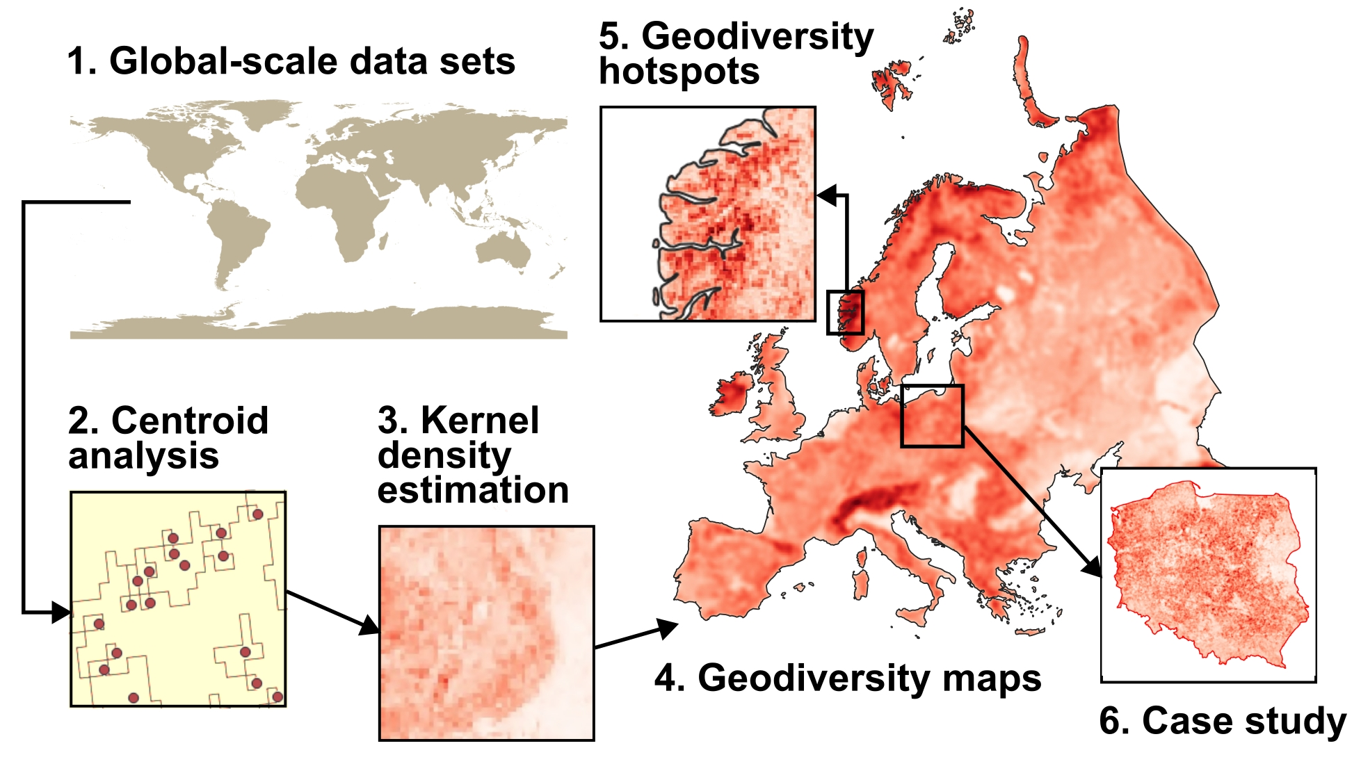
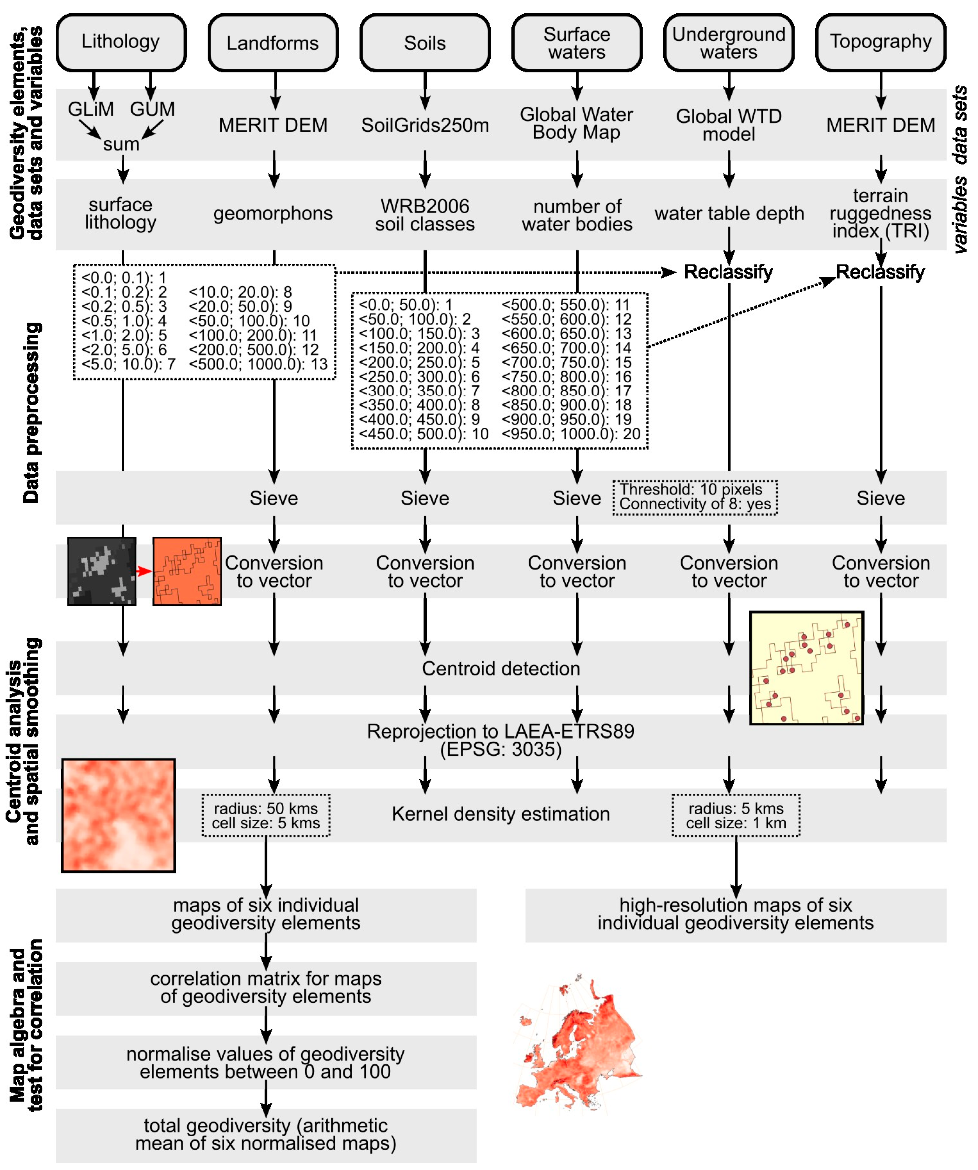
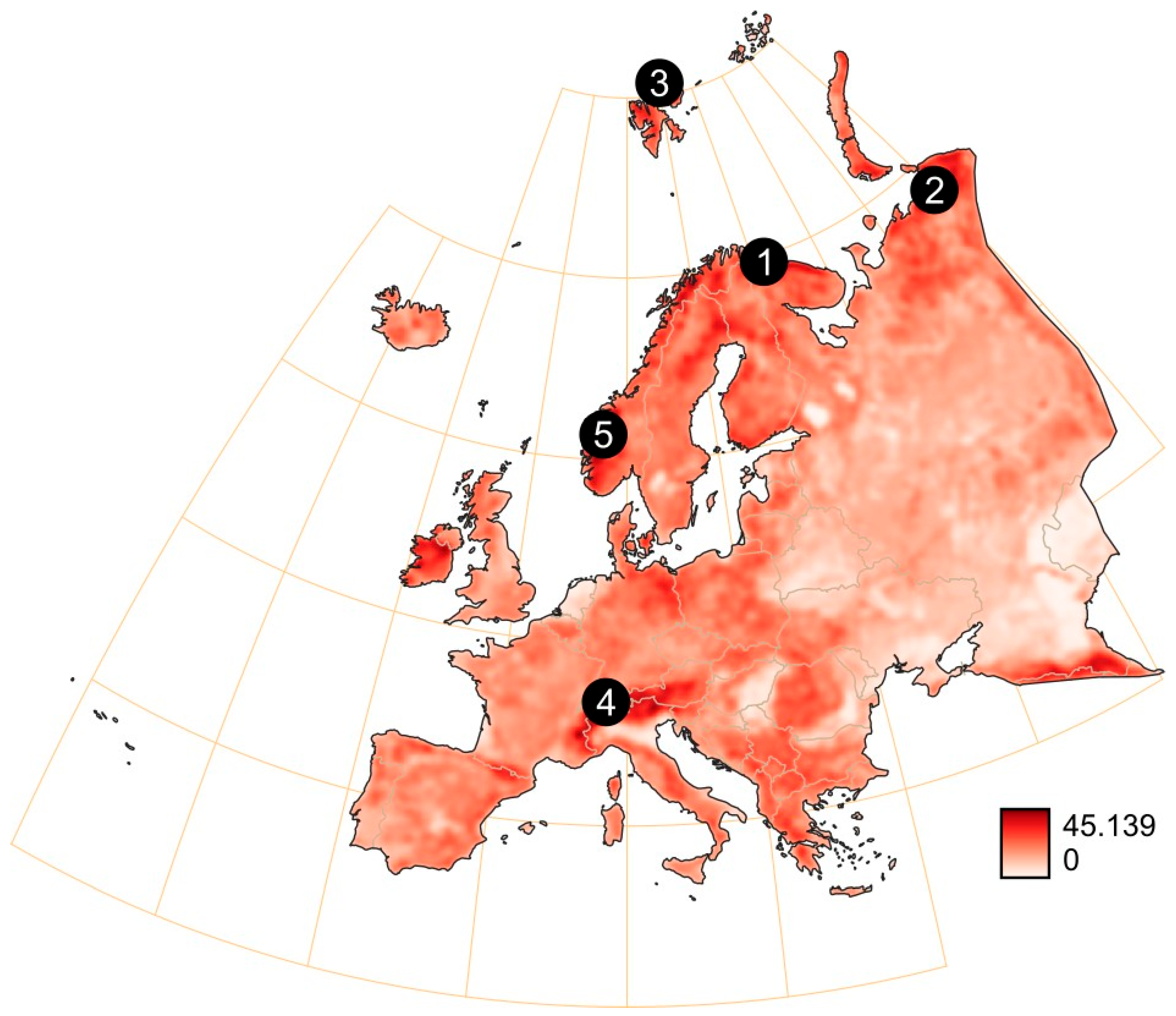
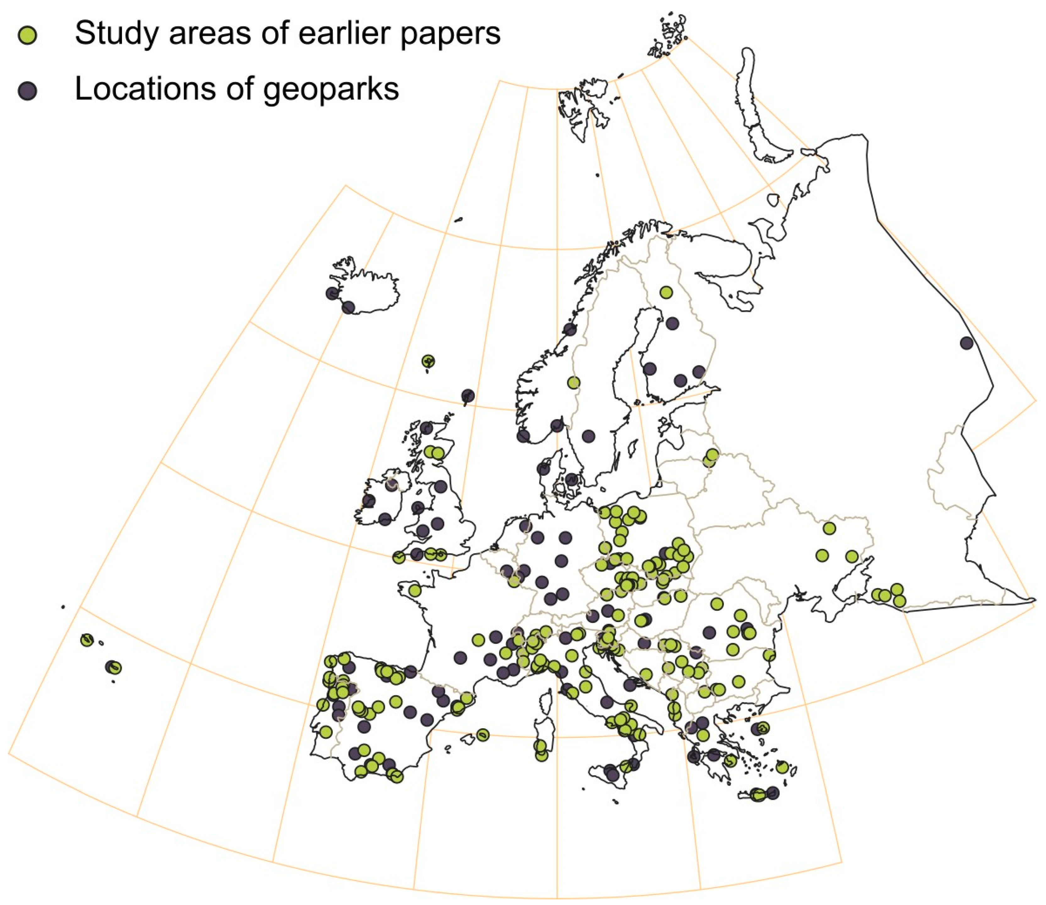
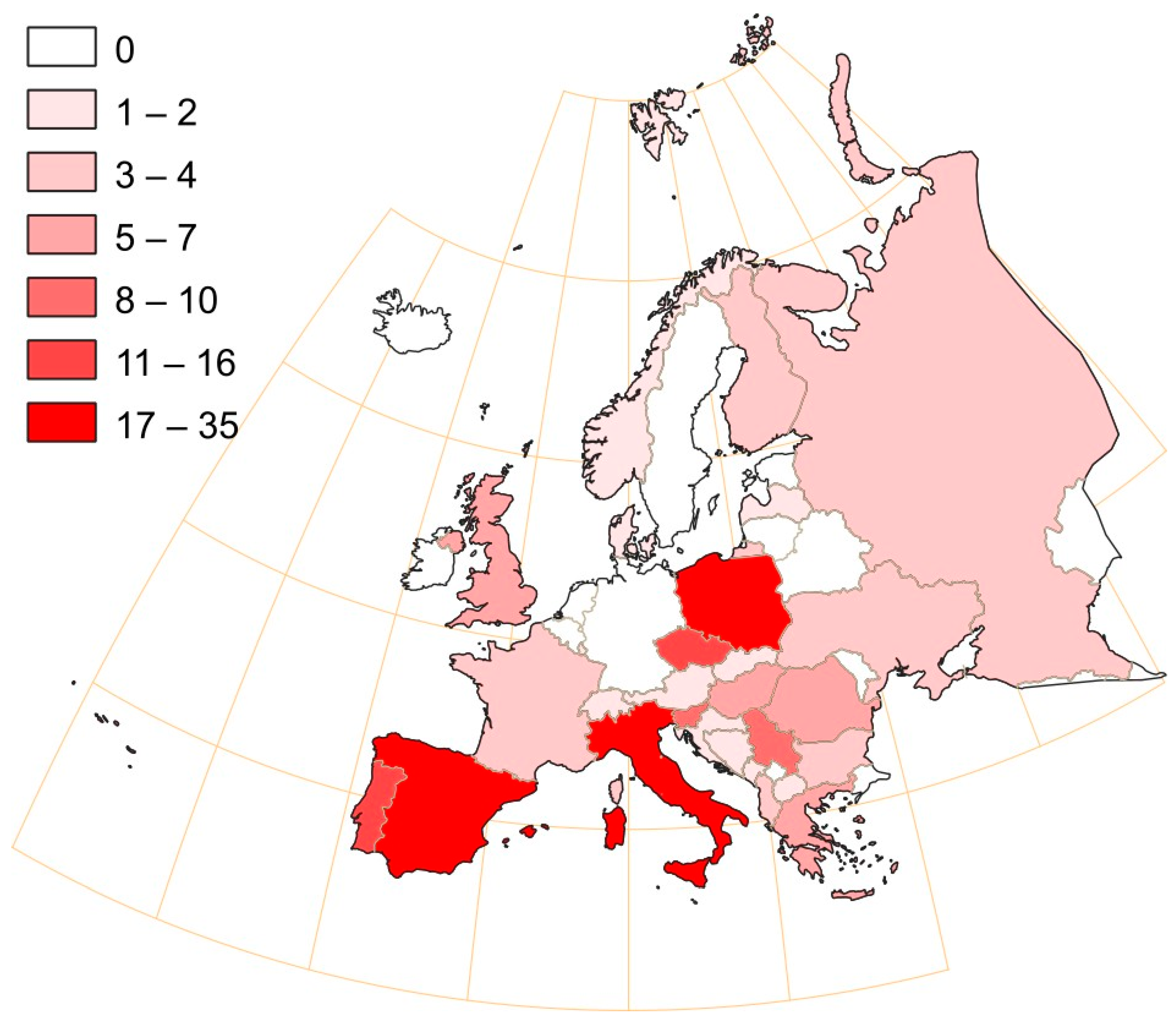
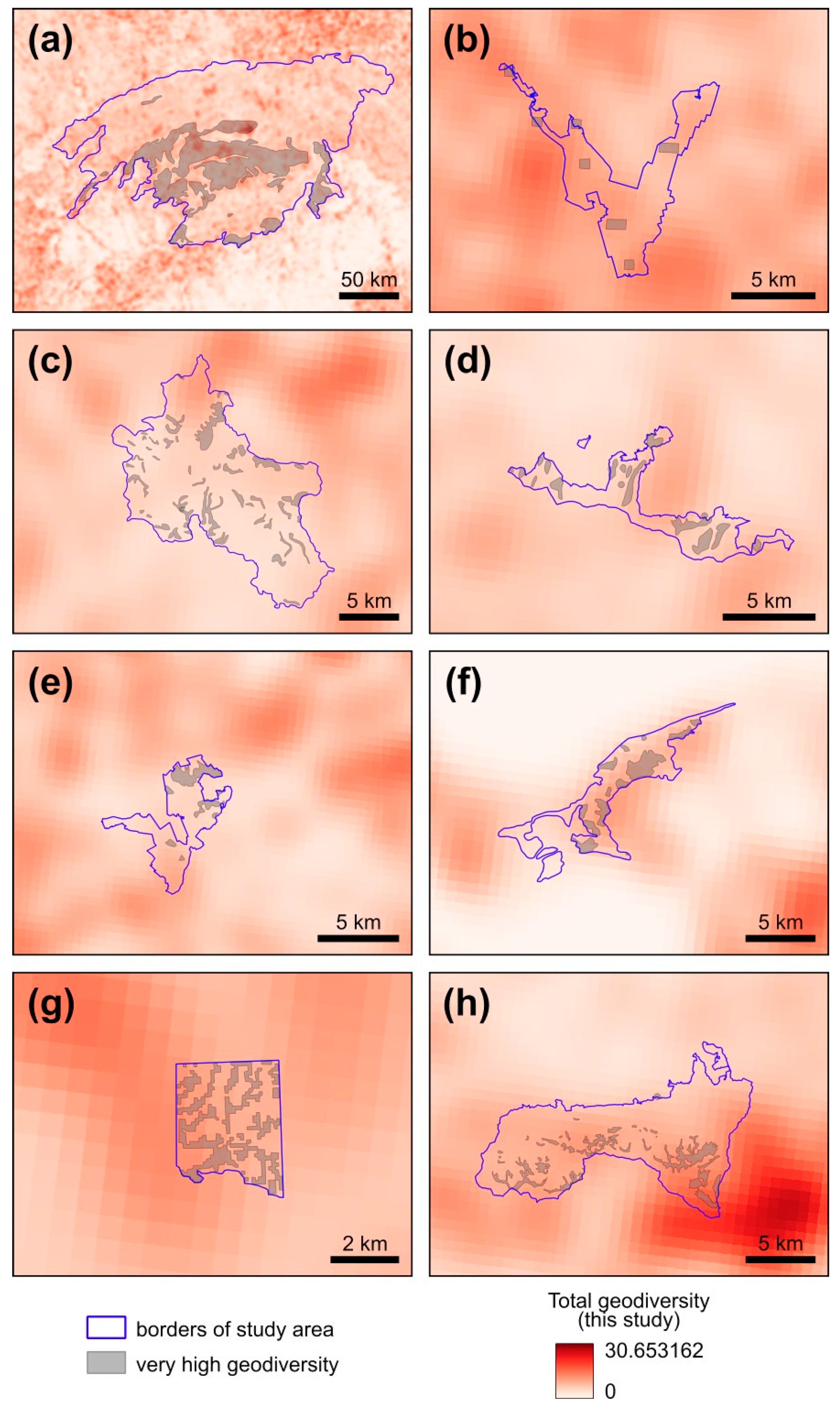
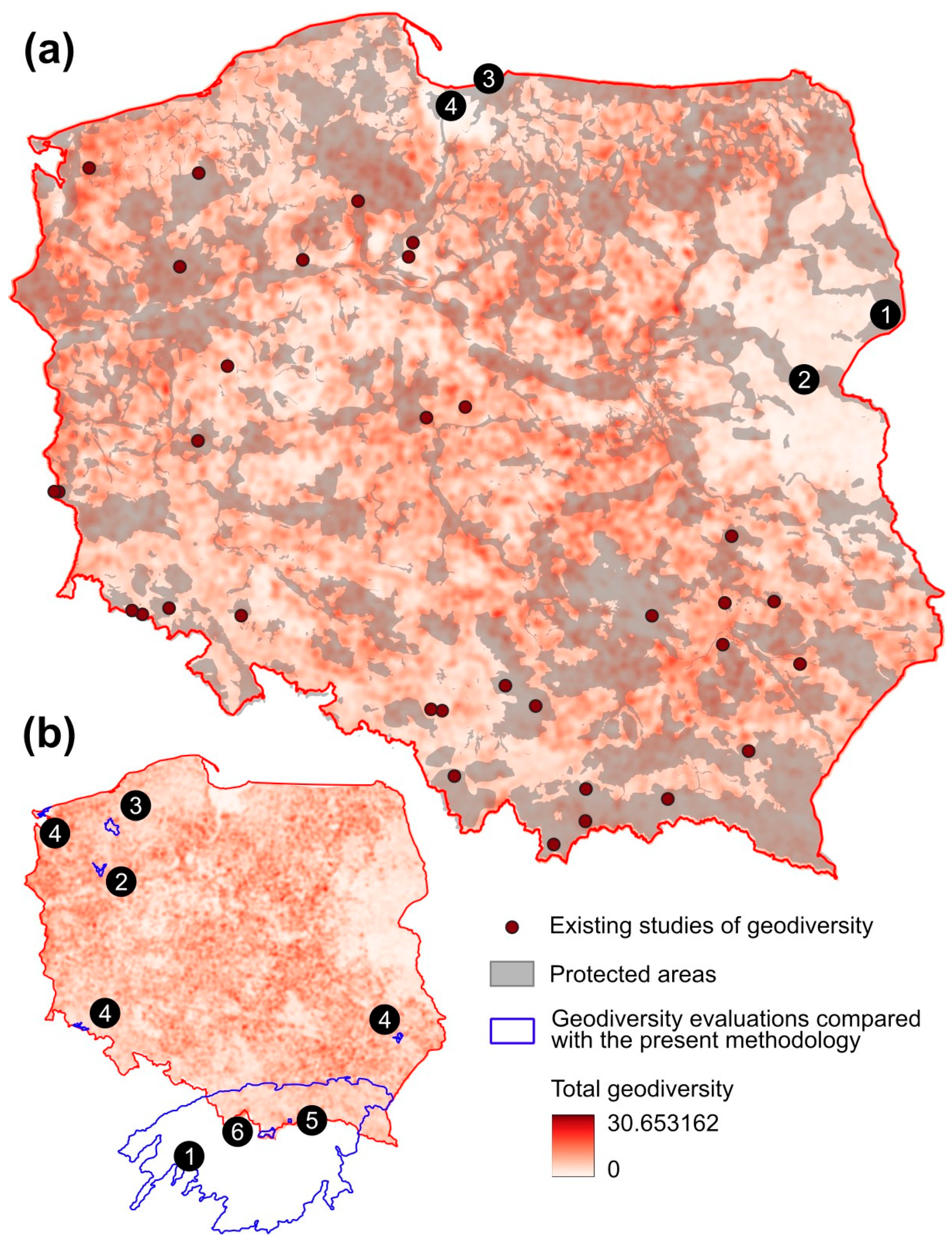
Table 1.
Input data for the evaluation of geodiversity in the present study.
| Geodiversity Feature | Parameter | Resolution/Scale | Sources and Algorithms |
|---|---|---|---|
| Geomorphodiversity (diversity of landforms) | geomorphons | angular resolution of three seconds | MERIT DEM [26] and r.geomorphon [27] |
| Hydrological diversity | number of individual water bodies | angular resolution of three seconds | Global Water Body Map [28] |
| Hydrogeological diversity | depth of the groundwater table | angular resolution of 30 s | water table depth data set [29] |
| Lithological diversity | diversity of lithological units | 1:3,000,000 | Global Lithological Map [30] and Global Unconsolidated Sediments Map Database [31] |
| Soil diversity | soil classes of the World Reference Base classification system | ground resolution of 250 m | SoilGrids250m [32] |
| Topographic diversity | terrain ruggedness index (TRI) | angular resolution of three seconds | MERIT DEM [26] and the algorithm by Riley et al. [33] |
Table 2.
Correlation coefficient matrix among the geodiversity variables used in the present study, calculated from the high-resolution maps included in Supplementary Materials S1.
Table 2.
Correlation coefficient matrix among the geodiversity variables used in the present study, calculated from the high-resolution maps included in Supplementary Materials S1.
| Geomorphology | Hydrology | Hydrogeology | Lithology | Soils | Topography | |
|---|---|---|---|---|---|---|
| Geomorphology | 1 | 0.089891 | 0.025250 | −0.052276 | −0.040580 | 0.095918 |
| Hydrology | 0.089891 | 1 | 0.071646 | −0.075945 | 0.038403 | −0.014773 |
| Hydrogeology | 0.025250 | 0.071646 | 1 | −0.045082 | −0.042982 | 0.271481 |
| Lithology | −0.052276 | −0.075945 | −0.045082 | 1 | 0.058896 | 0.009629 |
| Soils | −0.040580 | 0.038403 | −0.042982 | 0.058896 | 1 | −0.102918 |
| Topography | 0.095918 | −0.014773 | 0.271481 | 0.009629 | −0.102918 | 1 |
Table 3.
Lists of features used in earlier mesoscale geodiversity assessments on the territory of Poland.
Table 3.
Lists of features used in earlier mesoscale geodiversity assessments on the territory of Poland.
| Study | Geomorphology | Hydrology | Hydrogeology | Lithology | Soils | Topography | Other Geodiversity Features |
|---|---|---|---|---|---|---|---|
| [15] | + | + | + | land cover | |||
| [69] | + | + | + | ||||
| [70] | + | + | + | + | + | geoecology | |
| [71] | + | + | + | biodiversity, cultural assets, erratic boulders | |||
| [72] | + | + | + | + | climate | ||
| [73] | + | + | + | + | climate, land cover |
Disclaimer/Publisher’s Note: The statements, opinions and data contained in all publications are solely those of the individual author(s) and contributor(s) and not of MDPI and/or the editor(s). MDPI and/or the editor(s) disclaim responsibility for any injury to people or property resulting from any ideas, methods, instructions or products referred to in the content. |
© 2023 by the author. Licensee MDPI, Basel, Switzerland. This article is an open access article distributed under the terms and conditions of the Creative Commons Attribution (CC BY) license (https://creativecommons.org/licenses/by/4.0/).
Share and Cite
MDPI and ACS Style
Wolniewicz, P. Quantifying Geodiversity at the Continental Scale: Limitations and Prospects. Resources 2023, 12, 59. https://doi.org/10.3390/resources12050059
AMA Style
Wolniewicz P. Quantifying Geodiversity at the Continental Scale: Limitations and Prospects. Resources. 2023; 12(5):59. https://doi.org/10.3390/resources12050059
Chicago/Turabian StyleWolniewicz, Paweł. 2023. "Quantifying Geodiversity at the Continental Scale: Limitations and Prospects" Resources 12, no. 5: 59. https://doi.org/10.3390/resources12050059
Note that from the first issue of 2016, this journal uses article numbers instead of page numbers. See further details here.