1. Introduction
Since the first oil price shock in 1973, theoretical and empirical studies have investigated the relationship between economic activity and oil prices due to its significance (Hamilton, [
1,
2,
3]). The conclusions of the seminal study by Hamilton [
1] aroused controversy regarding the effect of oil prices on macroeconomic indicators. Through this analysis, he demonstrated the effect of oil prices on the US economy as a whole. Herrera and Hamilton [
4] discovered that oil price shocks have a larger impact on the economy and that monetary policy cannot prevent the contractionary effects of oil price shocks. In addition, Baumeister and Hamilton [
5] determined that oil supply shocks had a higher and more significant effect on economic activity than oil demand shocks. In addition, Baumeister and Peersman [
6] argued that oil supply shocks result in significant macroeconomic effects over time and that supply shocks explain a portion of the volatility in the real price of oil in the United States. In addition to the global economic expansion, Kilian [
7] found that the effects of oil shocks on macroeconomic indicators vary qualitatively and quantitatively depending on the source of the shock.
Indeed, the impact of oil price changes on macroeconomic indicators has been extensively studied, with some research focusing on specific macro indicators such as the impact of oil price fluctuations on economic growth and inflation rate (Barsky and Kilian [
8], Kilian [
9]; Hamilton [
10]; Nasir et al. [
11]). There is also a considerable body of research that investigates the relationship between oil prices and macroeconomics in oil-importing economies, either by examining the impact of oil demand and supply shocks on economic activity or the influence of oil price fluctuations on the global economy (Kilian [
9]; Baumeister and Peersman [
6]; Baumeister and Hamilton [
5]).
Although it is claimed in the literature that increases in oil prices cause negative and positive effects on oil-importing and oil-exporting countries, respectively, the mechanisms of the effects remain unclear. If an increase in oil prices occurs through the mechanism of wealth transfer from an oil-importing country to an oil-exporting country, then it can be said that it influences current account imbalances through trade or valuation channels. An increase in oil prices can lead to the depreciation of the currencies of oil importers, deterioration in current account balances, and a decrease in consumption, causing wealth transfer from oil importers to oil exporters through the trade channel. On the other hand, asset prices may change due to supply shocks through oil demand or the valuation channel, resulting in an increase in oil prices and a drop in the prices of assets in oil-importing countries relative to asset prices in oil-exporting countries, leading to temporary current account imbalances in both countries (Kilian et al. [
12]; Allegret et al. [
13]; Bodenstein et al. [
14]).
The literature demonstrates that an increase in oil prices has a positive impact on oil-exporting countries and a negative one on oil-importing economies, and that oil supply shocks affect the economy based on their location on the international oil market. In general, the method by which these impacts are conveyed remains obscure; hence, the size, timing, and even direction of the consequences of such shocks remain uncertain. However, a proper analysis of the effects of oil shocks over time is highly dependent on the sources of these shocks as well as the circumstances of countries; consequently, the effects of these shocks are likely to fluctuate over time. Numerous studies have utilized TVP-VAR methodology (Chien-Chiang et al. [
15]; Balli et al. [
16]; Lee and Olasehinde-Williams [
17]). Hence, the purpose of this study is to contribute to the literature on analyzing the effects of oil shocks on the trade balance in a time-varying framework by examining the differences in oil shock sources. To this end, we select the economy of Saudi Arabia as the largest producer and net exporter, and most significant player, on the global oil market. In addition, the oil sector contributed approximately 32.5 percent (on average) to the size of Saudi Arabia’s GDP from 2011 to 2020. (GCC-STAT [
18]). According to our knowledge, no study has been conducted on the impact of oil shocks on Saudi Arabia’s economy in the context of the time-varying parameters of such shocks.
Our results indicate that oil price shocks have more profound effects compared with oil production shocks, whether global supply or Saudi supply, and are unstable over time. Yet, we found that the effects of global oil production shocks were significant for the entire period of analysis and were greater than the effects of Saudi oil production shocks, which were not significant for most of the period. Further, the Saudi Arabian trade balance responded negatively to global oil supply shocks.
In this context, this study contributes to the literature on the interaction between oil shocks and macroeconomics in several respects. First, the primary goal of this research is to examine the possible time-varying effects of oil shocks on Saudi Arabia’s external balance. Second, unlike earlier research, we employ quarterly time series data, which allows us to give clear insights into the impacts of oil shocks. Third, we use the time-varying parameter vector autoregression model with stochastic volatility (TVP-VAR) to describe the dynamics of oil shocks in a flexible and resilient manner. Fourth, we differentiate between oil price shocks and oil production shocks, which gives us a detailed understanding of the Saudi economy’s sensitivity to oil shocks. Fifth, we distinguish between the amount of domestic oil production in Saudi Arabia and the amount of global oil output excluding Saudi Arabian oil production. Furthermore, while limited empirical evidence has acknowledged the significant impact of oil shocks on Saudi Arabia’s economics, this is the first attempt, to the best of our knowledge, to investigate the time-varying effects of oil shocks on Saudi Arabia’s trade balance by distinguishing the types of oil shocks [
19].
The remainder of this study is organized as follows:
Section 2 reviews the findings of the previous studies in this field.
Section 3 describes the TVP-VAR model and data.
Section 4 presents the empirical results of time-varying responses and forecast-error decompositions to quantify the impact of oil shocks on the trade balance of Saudi Arabia. Finally, the conclusions and policy implications are presented in
Section 5.
2. Review of Previous Studies
There is an abundance of literature that has investigated the interaction between oil shocks and macroeconomic indicators. This literature has examined the relationship using different methods in diverse contexts. However, very few studies have yet been conducted to examine the effects of oil shocks on the economics of the world’s largest net oil exporters, such as the economy of Saudi Arabia.
Most scholarly research has found that oil price shocks might have a great deal of influence on economic activity. Many studies have focused on advanced economies or oil-importing countries, specifically, the United States prior to its oil production. In this context, Hamilton [
1] found that oil price shocks were a significant contributing factor in most US economic recessions until 1972. In another study, Hamilton [
3] showed that oil price shocks played a significant role in the experience of the 2007–2008 recession. Work developed by Bjørnland et al. [
20] emphasized the important role of fluctuations in oil prices as a frequent source of US macroeconomic volatility and instability. In an empirical study of China as an emerging economy and the United States and Japan as developed economies, Taghizadeh-Hesary and Yoshino [
21] examined the impact of oil price movements on economic growth and inflation. They found that oil price fluctuations significantly and negatively impact economic growth. The effect on inflation in China was milder than in Japan and the United States. This led them to conclude that the negative impact was due to the fact that these were countries that depend on imported oil. Based on data from Thailand, Rafiq et al. [
22] confirmed that oil price fluctuations have a negative and important impact on the growth rate of the GDP and other macroeconomic variables.
Some empirical studies have also focused on oil-exporting countries. Bergholt [
23], for example, concluded that oil sector activities contribute to macroeconomic volatility for an oil exporter in a small open economy. Snudden [
24] showed that external shocks in oil prices lead to an increase in GDP through an increase in net exports in oil-exporting economies. Husain et al. [
25] noted that oil price fluctuations affect the economic cycle in countries where the size of the oil sector is large for the economy and where oil price changes affect macroeconomic fluctuations through their impact on fiscal policy. By developing a new Keynesian model for assessing oil price shocks, Bergholt et al. [
26] argued that oil price movements are an important source of macroeconomic volatility in Norway.
In contrast to the literature mentioned above, there are also studies that have examined the asymmetric impact of oil price shocks on the macroeconomy or on some of its indicators. For instance, Raheem [
27] tested the asymmetric effect of oil price changes on macroeconomics. By decomposing oil price changes into positive and negative shocks, an asymmetric effect was reported in high-trading economies (China and Germany) and in oil-exporting economies (Russia and Canada) in the long term, while in oil-importing economies (US and India) the asymmetric effect was in the short term. Similarly, Akinsola and Odhambo [
28] concluded that an asymmetric effect of oil price shocks on macroeconomics is limited to the long run in seven oil-importing economies in sub-Saharan Africa.
In fact, there is another dimension that has been identified in the empirical literature that distinguishes between oil shocks in terms of the source of the shock, i.e., demand or supply shocks. Kilian [
7], for example, noted that not all oil shocks have a similar effect on a country’s macroeconomics. Baumeister and Peersman [
6] reported the same conclusions. They also found that oil supply shocks represent a part of the fluctuation in the real price of oil and therefore play a greater role than oil demand shocks.
Moreover, due to their direct impact on the external balances, recent literature has focused on the impact of oil shocks on external imbalances as one of the macroeconomic indicators, whether in oil-exporting or oil-importing economies. Based on data for Malaysia as a net exporter, Japan as a net importer, and Singapore as an oil refiner, Le and Chang [
29] reported a long-run causal relationship between oil price and the total oil and non-oil trade balances in Malaysia and Japan, while the evidence for this was insufficient in Singapore. They concluded that an increase in oil prices was beneficial for exporters, while it was the opposite for importers. For the oil refinery economy, oil price shocks had a negligible impact on trade balances and their oil and non-oil components. According to Kilian et al. [
12], the oil demand and supply shocks affected the external balance. In addition, they found that the overall effect of the oil shocks on the trade balance depends not only on the source of the shock but also on the response of the non-oil trade balance, whether for oil exporters or importers.
Ozlale and Pekkurnaz [
30] illustrated that the current account responds negatively and significantly to oil price shocks in the Turkish economy. Yalta and Yalta [
31] highlighted the same findings, namely that fluctuations in oil prices have important effects on Turkey’s current account. For India, Tiwari et al. [
32] concluded that positive oil price shocks have a significant effect on the trade balance. Similarly, Anand and Zhang [
33] illustrated that oil prices negatively affect the current account in Pakistan, while, in a highly oil-export-dependent economy like Nigeria, Chuku et al. [
34] found that current account dynamics respond positively to positive oil price shocks.
On the other hand, Jibril et al. [
35] found that the asymmetric effect of oil prices on trade balances depends on the source of the shock. They concluded that an increase in oil prices due to global demand leads to the deterioration of trade balances for oil importers, in contrast to their improvement for oil exporters. Also, Baek and Kwon [
36] noted that oil prices have asymmetric effects on the trade balance in six major African economies. Rafiq et al. [
22] investigated the asymmetric impact of oil shocks on external balances in 28 oil exporters and 40 oil importers. They argued that an oil price decrease has a positive effect on oil exporters and a negative effect on oil importers, and this is because the effect of quantity outweighs the effect of price.
Using the TVP-VAR model in Canada’s diversified economy, Gnimassoun et al. [
37] concluded that the current account responded to oil demand shocks significantly and positively due to the oil trade balance surplus, while oil supply shocks had no effect. Also, they indicated that the implications of oil shocks on the current account depend on the oil price intensity and the degree of sectoral diversification of the economy. Nasir et al. [
38] examined the implications of oil price shocks on the BRICS economies. Their empirical results showed that the internal and external balances of the BRICS economies responded asymmetrically and very differently to oil price shocks, whether oil exporters or importers, and even within. They pointed out that the increased dependence on oil makes such economies more vulnerable to the implications of oil price shocks. In another study, Nasir et al. [
11] found that oil price shocks have important positive effects on GDP, trade balance stability, and inflation in the economies of the GCC. They concluded that the transmission mechanism of shocks was considerably different across these economies in terms of intensity. Mohaddes, et al. [
39] concluded that a slowdown in the global economy has a significant and long-lasting impact on the economic growth of Saudi Arabia and oil prices.
More recently, Balli et al. [
16] showed that the trade balance responded to oil shocks very differently between China as an importer and Russia as an exporter, and that the source of the shock was important for understanding its implications. Abu Eleyan et al. [
40] analyzed the impact of oil price shocks on trade balances in the ASEAN-5 economies, i.e., Malaysia, Indonesia, the Philippines, Singapore, and Thailand. They also indicated that oil price shocks have time-varying and significantly different effects on trade balances between economies due to their distinct positions in the oil trade as oil importers, exporters, or refiners.
Saudi Arabia ranked third in crude oil production globally in 2021, with production reaching 9.125 million barrels per day, accounting for approximately 13.10 percent of global production. Due to the so-called “great shutdown” caused by COVID-19 in 2020, crude oil production decreased by 6.1% and oil exports decreased by 5.4% [
19]. In addition, Saudi Arabia’s nominal GDP in 2021 exceeded 833.5 billion US dollars, making it the eighteenth largest economy in the world and 0.87 percent of the global economy.
Overall, economic growth in particular, and development in general, in Saudi Arabia are closely related to the demand-driven fluctuations in oil prices and oil supply shocks, as a result of upswings or downturns in global growth. This is because the Saudi economy is mainly dependent on oil revenues. In 2009, when oil prices fell by about 40% after the 2008 global financial crisis, real economic growth contracted to an average of −2.1% from a growth rate of about 7.98% in the previous five years. Also in 2014–2019, growth declined to an average of 1.9% from an average of 5.8% in the previous four years as a result of the collapse in oil prices by nearly 50% from their peak. The recovery of oil prices has been slow and partial since the collapse of 2014, even with OPEC restrictions in the period 2017–2019 in order to restore stability in prices. In 2020, with the major global shutdown to counter the spread of COVID-19, oil prices collapsed to USD 29.6 per barrel in the second quarter of 2020, the lowest level since 2004, as this led to the plummet of economic growth to an average of −4.1% in Saudi Arabia, while the global economy contracted by −3.1% and −2.1% in emerging markets and developing economies, respectively. However, Jouini and Gaaloul [
41] argued that the economic growth of the GCC interacts significantly with fluctuations in oil prices. By decomposing oil prices into increases and decreases, real GDP responses to negative oil price shocks were found to be higher than the responses to positive oil price shocks in the long run.
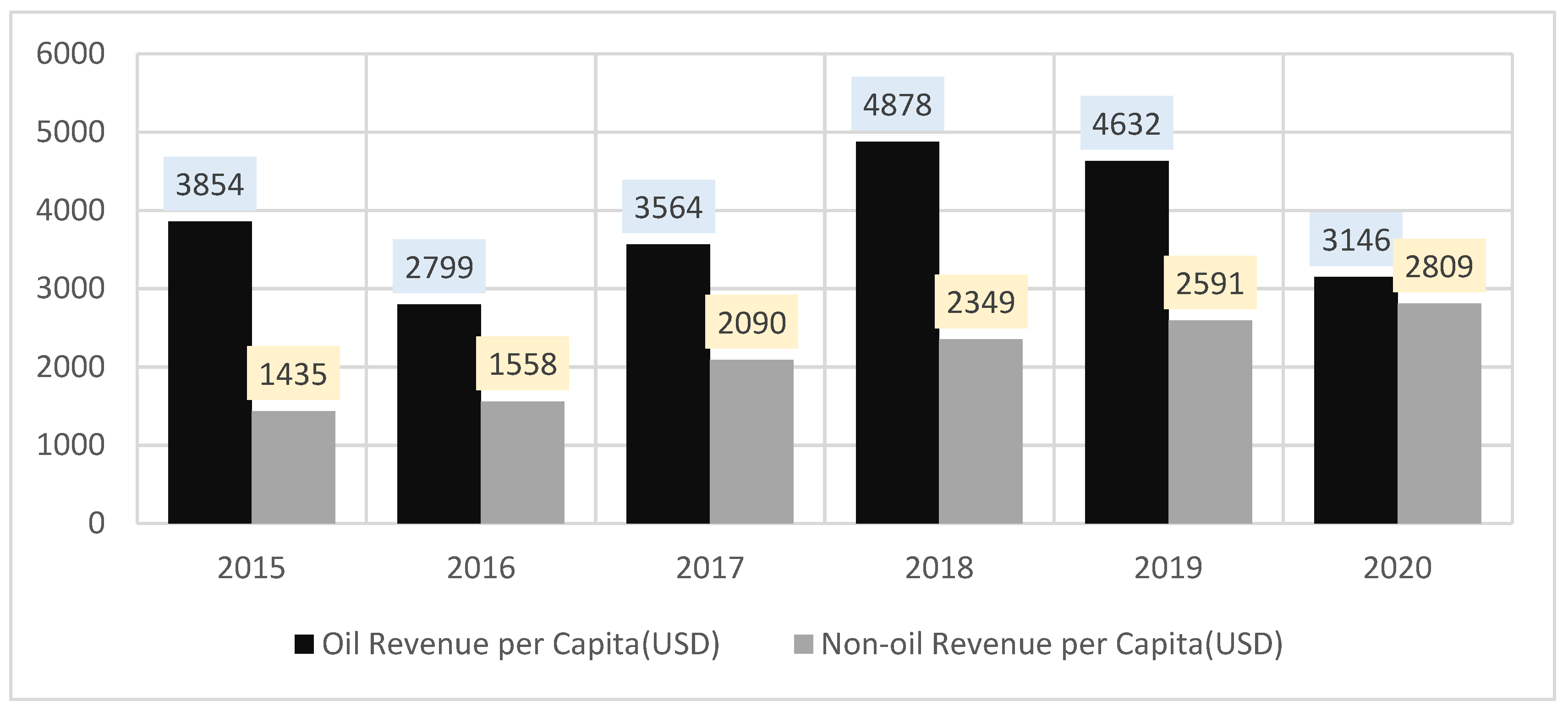
Despite the attempt to diversify sources of income in Saudi Arabia, oil revenues are still higher than non-oil revenues, meaning the degree of dependence on oil is still huge.
Figure 1 depicts this phenomenon. However, differences in the level and degree of dependence of the economy on oil can lead to very different effects on the response to oil shocks. Moreover, the empirical literature ignores the instability of oil dependence and its implications. Therefore, there is merit in studying the time-varying effects of oil shocks on the macroeconomics of Saudi Arabia.
The empirical literature outlined above indicates that estimating and analyzing the effects of oil shocks on the trade balance is a very difficult task, since differences in the source of oil shocks are likely to affect economies in very different ways, whether in oil-exporting or oil-importing economies. Furthermore, the majority of the literature does not account for the time-varying effects of oil shocks on the macroeconomy, implying that the estimated parameters remained constant throughout the analysis period. Accordingly, our study bridges the gap in the literature by estimating the time-varying effects of oil shocks on the external balance of Saudi Arabia using the TVP-VAR model. To our knowledge, this is the first attempt to study the impact of oil shocks in Saudi Arabia in the context of the time-varying parameters of such shocks.
4. Empirical Results and Discussion
This section presents how the TVP-VAR model is applied to the data of our study in order to analyze the effects of oil shocks on the macroeconomics of Saudi Arabia. To accurately estimate time-varying parameters in terms of unobserved latent variables, a Bayesian approach based on the Markov Chain Monte Carlo (MCMC) algorithm is employed. By breaking the estimation sample into smaller portions, this strategy is very effective for dealing with nonlinearities and large parameter space dimensions (Nakajima [
51]; Balli et al. [
16]; Abu Eleyan et al. [
40]). The time-varying stochastic fluctuation causes the model to be non-normal state-space and nonlinear, which requires different sampling methods. Following Nakajima [
51], to sample the exact posterior density of stochastic volatility, we employ a multi-move sampler developed by Shephard and Pitt [
52] and Watanabe and Omori [
53].
To achieve convergence of time-varying parameters, a simulation is conducted by drawing 100,000 samples from the posterior distribution, where the initial 10,000 observations in the sample during the burn-in period are discarded.
Table 3 reports the descriptive statistics for the selected parameters of the TVP-VAR model based on MCMC estimation. From the results, it is found that the estimated posterior mean lies within the confidence intervals of 95 percent, and the Convergence Diagnostic (CD) test based on Geweke [
54] indicates that the null hypothesis of convergence to the posterior distribution is not rejected at the five percent level of significance. Moreover, most inefficiency factors for sampling are relatively low. Therefore, we can conclude that the MCMC method generates posterior draws efficiently and that the number of iterations is sufficient to converge the parameters of the estimated model. (To determine the optimal number of lags in the VAR, we utilized the Akaike Information Criterion (AIC). The same priors in Nakajima [
51] are applied in the TVP-VAR estimates.)
After investigating the convergence of the parameters, the time-varying responses to oil shocks are calculated based on the variance-covariance matrix of the TVP-VAR model. In
Figure 2,
Figure 3,
Figure 4 and
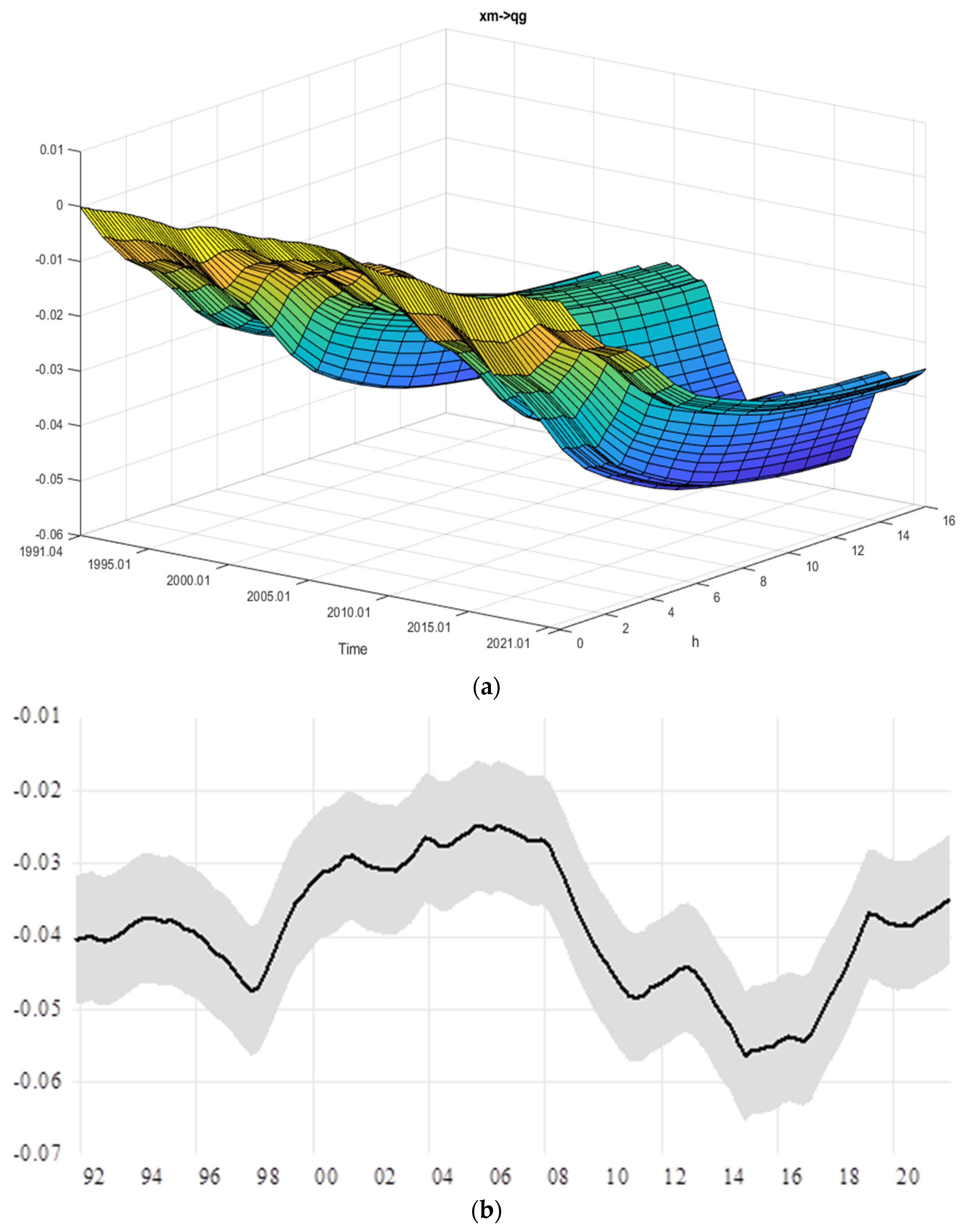
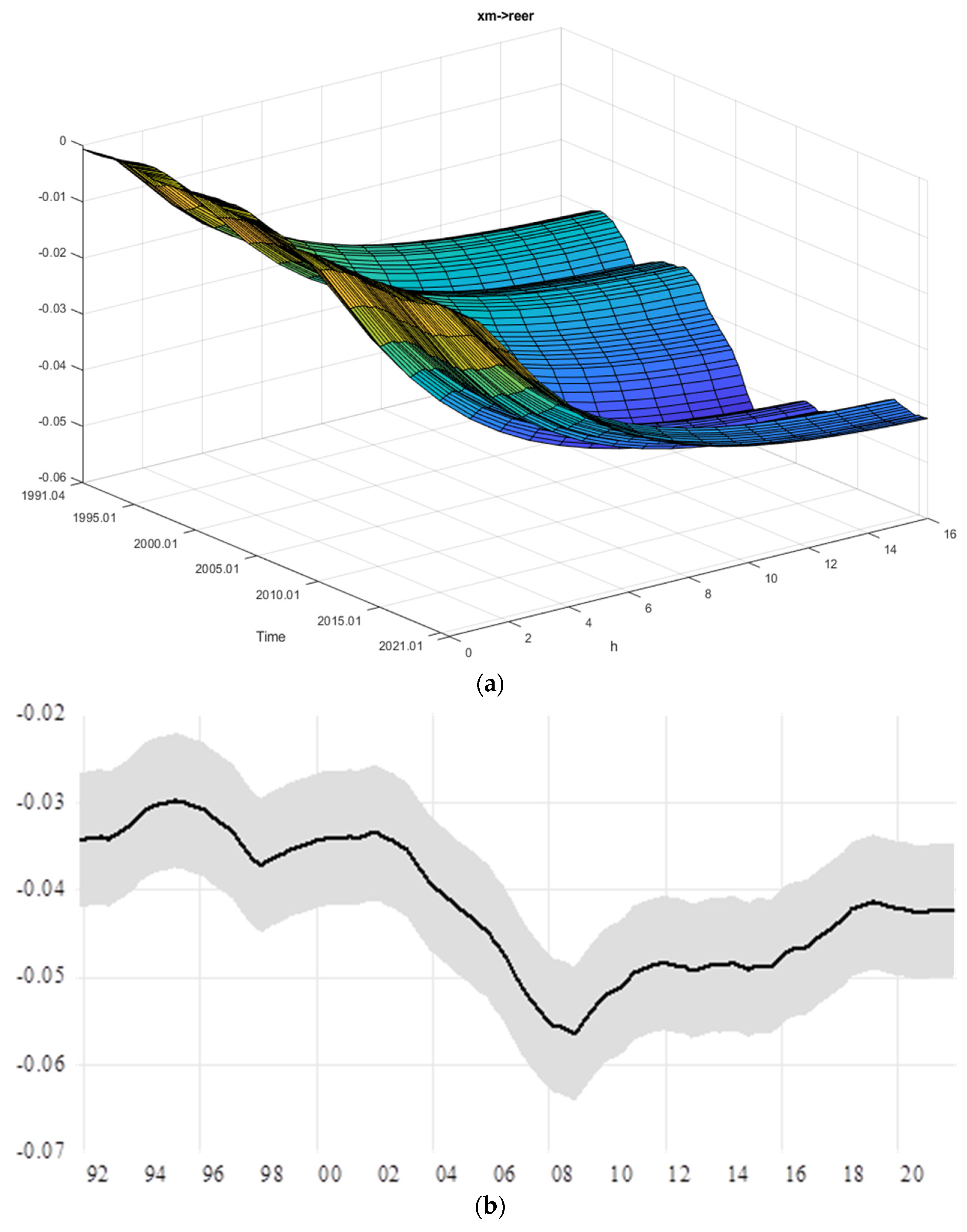
Figure 5, we plotted the cumulative time-varying responses of trade balance to the shocks based on two different illustrations. In each figure, panel (a) shows the surface plot including a three-dimensional representation of the cumulative responses for the time horizon t = 0 to 16, while panel (b) shows the accumulated responses over the sixteenth-quarter horizon, h = 16th, along with the confidence bands, in order to evaluate the significance of the shocks over the examined period.
The time-varying responses of the trade balance to global oil production shocks are presented in
Figure 2. It is worth reiterating that the global oil production variable does not contain domestic oil production in Saudi Arabia. Consistent with expectations, global oil supply shocks have a negative impact on the Saudi economy as the world’s largest net oil exporter over the whole analysis period. In addition, panel (b) of the figure implies that the responses are statistically significant for the whole analysis period. In terms of the magnitude of the impact of global oil supply shocks, the negative impact is more pronounced during periods of global crises and disruptions in the global oil market. This means that fluctuations in global oil production have a serious impact on the external balance of Saudi Arabia, the world’s largest net oil producer and exporter. The Saudi economy’s negative response to global oil supply disruptions appears to be closely associated with the collapse of global oil demand and consequently the huge fluctuations in real prices during and immediately after global crises.
One of the largest negative responses to global oil supply shock was recorded during the year 2006 due to the increasing trend in oil production and the global oil demand shock that doubled the oil price from USD 32.1 in the first quarter of 2004 to USD 68.6 per barrel in the third quarter of 2006 (see
Table 4), while the largest negative response occurred in the fourth quarter of 2014, coinciding with the start of what is known as the “great plunge”, when prices collapsed sharply from USD 106.4 in the second quarter of 2014 to USD 32.5 per barrel in the first quarter of 2016. Two other remarkable effects of the global oil supply shock occurred: the first was at the end of the 1990s in conjunction with the Asian and Russian financial crises, which dropped global oil prices to their lowest levels during the entire investigation period; the second coincided with the 2008 global financial crisis and the collapse of the real oil price from USD 120.7, its historical high in the second quarter of 2008, to USD 44 per barrel in the first quarter of 2009. Overall, the results show that the responses of Saudi Arabia to global oil supply shocks are not stable for most of the analysis period and depend on the magnitude and duration of the shocks. Thus, it is affected by fluctuations in global oil production.
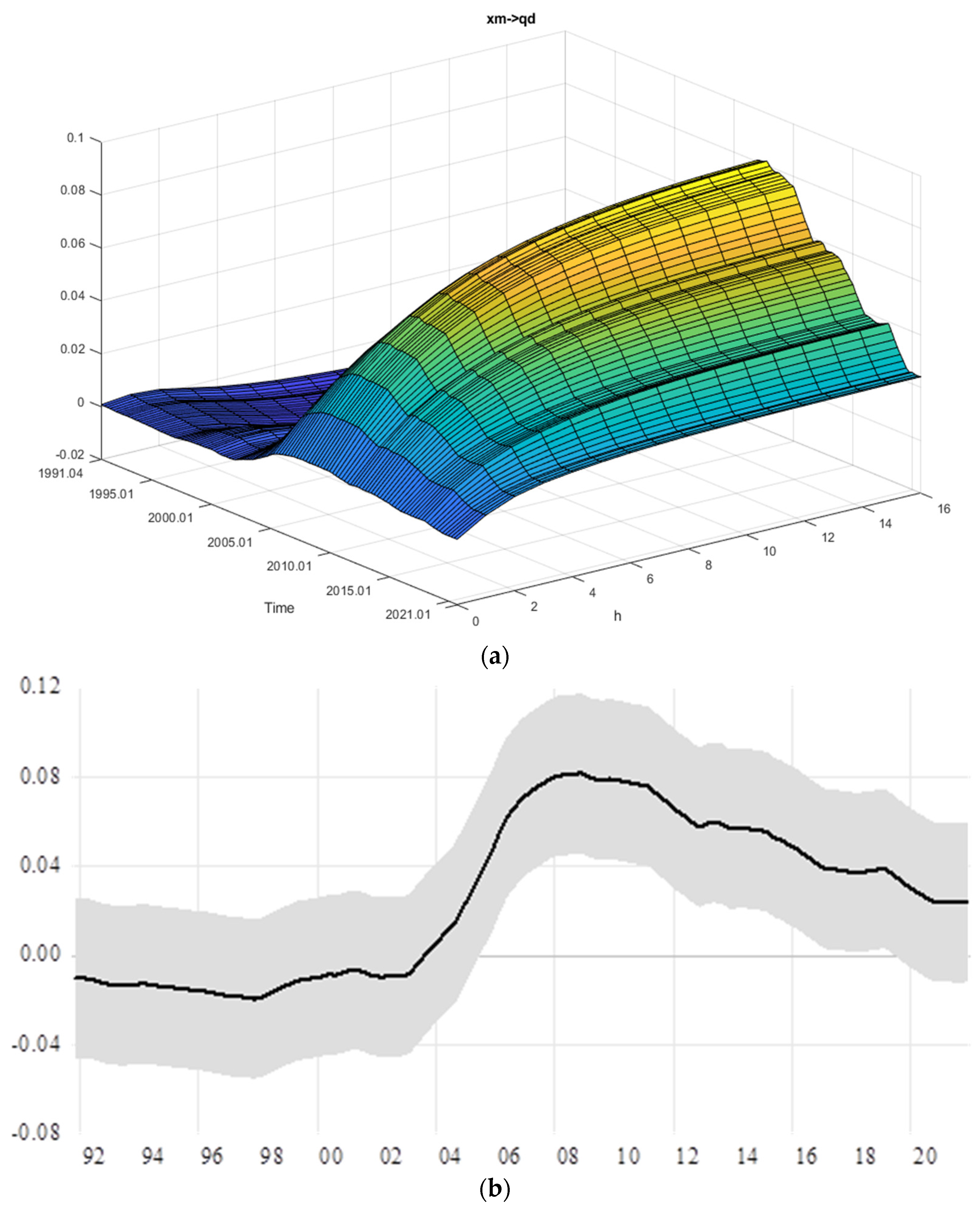
Figure 3 presents the time-varying response of the trade balance to the positive shocks in the domestic oil production of Saudi Arabia. The estimated response to changes in domestic oil production has an average value of 0.026 and ranges between 0.081 and −0.019 (see
Table 4). However, this effect is negative and small in magnitude until 2003: Q2 before becoming positive until the end of the period, as the global oil price increased about 3.4 times on average from before to after this quarter. After that time, there was a global tendency to increase oil production and thus increase the domestic production of Saudi Arabia to cover the growing global demand, as well as for the global price of oil to rise dramatically until it reached its highest level of USD 120 per barrel in 2008: Q2 before returning to fluctuations until the end of the period, but remaining above the average prices prior to 2003. Meanwhile, it is worth mentioning that the responses are not statistically significant during the investigation period except for the period 2006: Q4 to 2011: Q3, when it reached its highest level of 0.081 in 2008: Q4. In general, this period is associated with the highest level of average oil prices historically, despite the shock of the price collapse in 2009: Q1 to USD 44 per barrel, which coincided with the global financial crisis at the end of 2008. In addition, the responses tended to take a downward trend since 2011: Q4 until the end of the investigation period, and this may be attributed to the large fluctuations in prices and their collapse several times during this period, as it reached about USD 32.5 per barrel in 2016: Q1 and about USD 29 in 2020: Q2 during the COVID-19 pandemic; these are the lowest price levels since 2003. Furthermore, the recent US oil supply expansion revolution has consequences for other producers, particularly Saudi Arabia, prompting many oil producers to seek a cooperative effort to cut supply, notably by Saudi-led OPEC and OPEC Plus, in order to face price deterioration and weak global demand for oil.
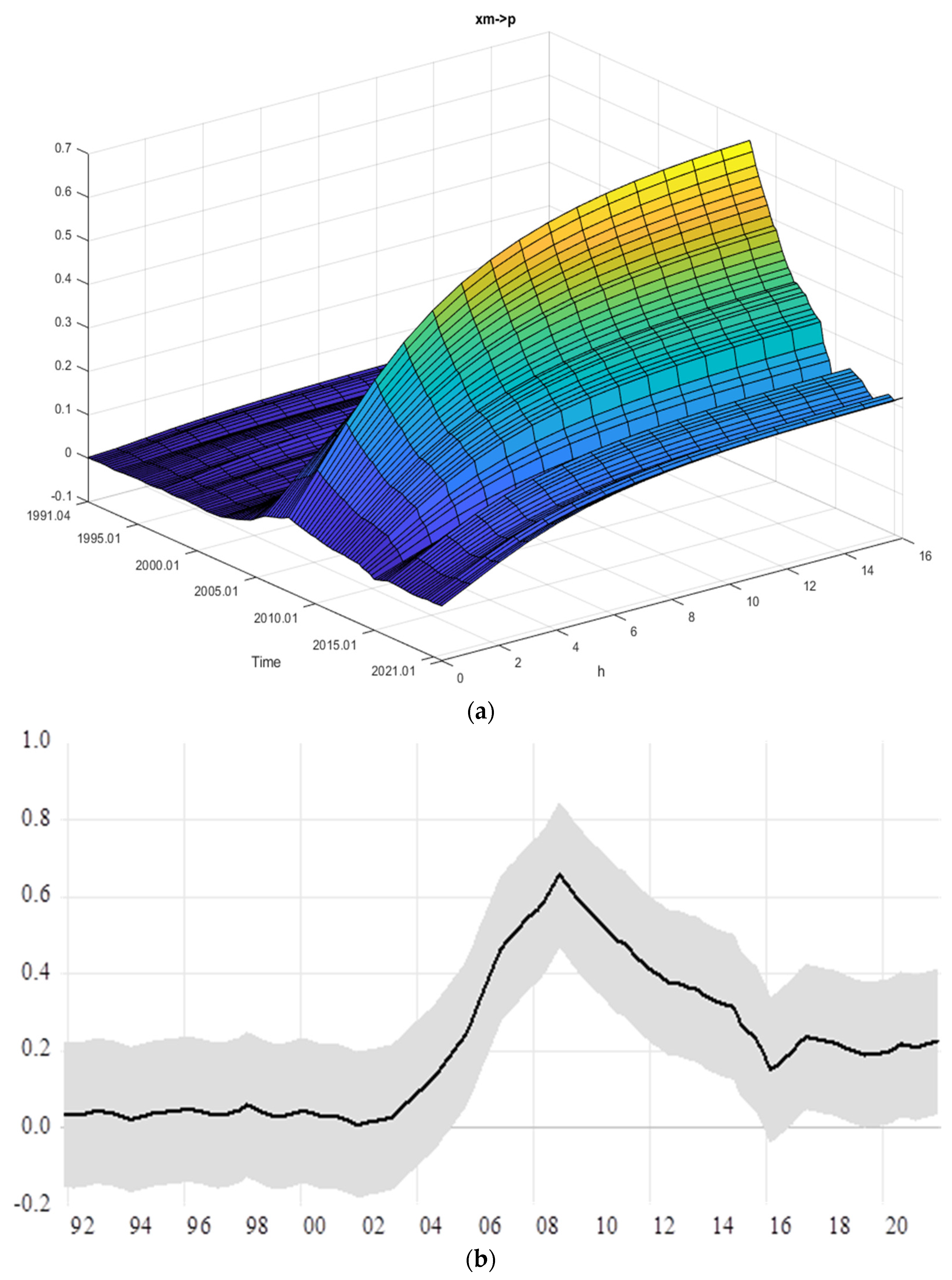
Figure 4 depicts the time-varying effects of oil price shocks on the trade balance of Saudi Arabia. The results show that oil price shocks have more pronounced impacts on the external balance of Saudi Arabia compared with oil production shocks, which is considered intuitive, as oil is the major source of Saudi exports. The responses did not change remarkably from the beginning of the period until the 2002: Q4 and were not indistinguishable from zero, as they reached their lowest value of 0.009 in 2001: Q4; when the global oil price fell below USD 20 per barrel. This might be attributed to the relative stability of global oil prices at their lowest historical levels, as the price of a barrel reached USD 20 on average, and at best it did not exceed USD 31 during this period. After that time, the value of the responses gradually increased until it reached a peak of 0.656 in 2008, when oil prices exceeded USD 110 per barrel in the second and third quarters of 2008. In addition, the estimated responses tended to decline dramatically from the peak until they reached 0.151 in 2006, which is the lowest value during this period, before they tended to remain relatively stable until the end of the analysis period. This is due to the huge fluctuations in the global oil price and its instability during that period, as prices collapsed to below USD 50 several times, most notably in 2009: Q1 and 2016: Q1 and below USD 30 in 2020: Q2. However, the average of the estimated responses is 0.212.
Furthermore, the impact of oil price shocks is found to be insignificant in most of the estimation period, but significant responses are reported from 2006: Q2 to 2012: Q4, during which the time crude oil price plateaued at approximately USD 83 per barrel on average and reached its peak in 2008: Q2 before its collapse and recovery again, exceeding USD 100 between 2011: Q1 and 2012: Q4. Therefore, one can conclude that the macroeconomics of a major and net oil-exporting country like Saudi Arabia is highly sensitive to fluctuations in oil prices compared with fluctuations in oil supply.
Finally,
Figure 5 depicts the time-varying response of real exchange rate shocks on the trade balance. In line with expectations, the trade balance responded negatively and significantly to real exchange rate shocks during the period under analysis. It is worth noting that the largest negative effects of positive real exchange rate shocks on the trade balance occurred during the 2008 global financial crisis and the 1998 Asian financial crisis. This is due to the deterioration of the exchange rate of currencies of the trading partners against the Saudi riyal, thus leading to an overvaluation of the riyal against foreign currencies.
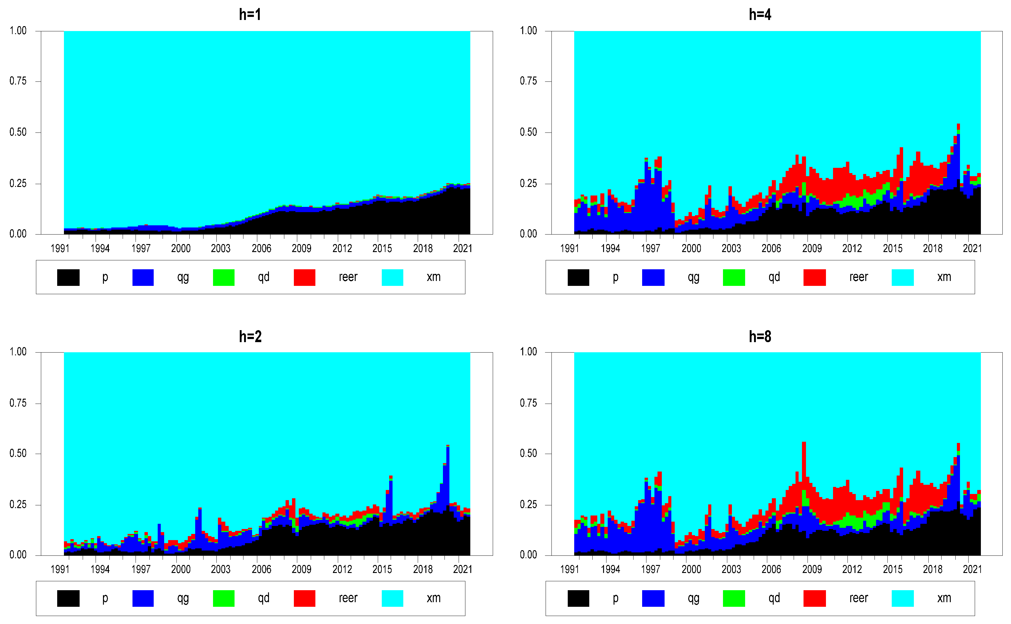
In addition to the impulse response analysis, the time-varying variance decomposition analysis is performed to assess the relative importance of oil and real exchange rate shocks in affecting the trade balance of Saudi Arabia.
Figure 5 presents the time-varying variance decompositions of the trade balance at h = 1, 2, 4, and 8 quarter-ahead horizons. In general, the results of the forecast error decomposition are consistent with the results of the time-varying impulse responses. Overall, it is worth noting that most fluctuations in the trade balance are explained by the own shock of the variable. However, it is observed that the explanatory power of other shocks fluctuates substantially over time.
The results of the variance decompositions at the horizon (h = 1) in
Figure 6 indicate that about 96.7% of the variation in the trade balance is explained by its own shocks in 1991: Q4, while oil price shocks explain about 1.95%. However, the explanatory power of trade balance shocks gradually declines with the increase in the forecast horizon, declining on average from 88.7% at h = 1 to 73.1% at h = 8 for the period under investigation. Indeed, the largest portion of prediction errors is explained by own shocks of trade balance at around 93.1% in the second quarter of 1999, coinciding with the Asian financial crisis, while the lowest explanatory power is reported in the fourth quarter of 2008, coinciding with the global financial crisis, at around 43.9%.
The explanatory power of oil demand shocks continued to be the second largest major contributor to trade balance variations, after its own shocks, and ranged on average between 9% and 10% across all horizons. At the same time, the contribution of oil demand shocks to the trade balance shocks increased dramatically over time, reaching a peak in the second quarter of 2020 at about 27.4%, which coincided with the collapse of global oil prices to less than USD 30 per barrel for the first time since 2004 due to the so-called “Great Lockdown” caused by the COVID-19 pandemic. Conversely, the lowest contribution was in the third quarter of 1999, which coincided with an increase in the oil price of about 75% compared with the first quarter of the same year, when the oil price was at its lowest level during the study period.
Similarly, with the increase in the prediction horizon from h = 1 to h = 8, the contributions of global oil production shocks excluding Saudi Arabia increased significantly from 1.67% to 8.46% and real exchange rate shocks from less than 1% to 7.28% to explain the variation in the trade balance of Saudi Arabia. Moreover, real exchange rate shocks showed the greatest impact on trade balance shocks of about 23.6% in the fourth quarter of 2008, which coincided with the global financial crisis, while the lowest impact was in the first quarter of 1997 and was less than 1%. Finally, it is remarkable that the explanatory power of Saudi oil production shocks remains very weak, whether in the case of an increase in the forecast horizon or over time.
By the end of the analysis period, most of the variation in the Saudi trade balance was explained by its own shocks (more than 73%), followed by oil price shocks (more than 9%), which remained at their level at all forecast horizons and increased over time, peaking with the great global lockdown caused by the COVID-19 pandemic. At the same time, the forecast error variance in the trade balance explained by shocks in the global oil production and the real exchange rate increased with the increase in the forecast horizon (from less than 2% to more than 7%), and their impact increased during global shocks, as in the global financial crisis of 2008 and the COVID-19 pandemic in 2020. The Saudi oil supply shocks have almost no explanatory power and remain less than 2% at all forecast horizons.
5. Conclusions and Policy Implications
Given Saudi Arabia’s importance as one of the world’s leading net oil producers and exporters, as well as its reliance on oil revenues for economic growth, this paper investigates the time-varying effects of oil shocks on its macroeconomics. In contrast to previous studies, we used the TVP-VAR model to develop a model for Saudi Arabia by distinguishing between global oil production shocks, excluding Saudi Arabia, and Saudi Arabian oil production shocks. This methodology allows us to quantify the time-varying effects of the three oil shocks and assess their explanatory power over time. Another unique feature of our study is that we used quarterly data from 1991: Q1 to 2021: Q4, allowing us to more accurately quantify the effects of oil shocks on trade balance.
Based on the empirical findings of the unit root test results with structural shifts, we can conclude that there is at least one significant structural break in all variables. This reflects the extent of variation in the impact of the three oil shocks and their transmission mechanisms to the Saudi economy in general during the period under analysis. The empirical results of the estimated time-varying parameters lead us to conclude that there are substantial differences in the response of the Saudi economy to the three oil shocks and to the real exchange rate shocks in general.
The results indicate that oil price shocks have more profound effects compared with oil production shocks, whether global supply or Saudi supply, and are unstable over time. Yet, we found that the effects of global oil production shocks were significant for the entire period of analysis and were greater than the effects of Saudi oil production shocks, which were not significant for most of the period. Further, the Saudi Arabian trade balance responded negatively to global oil supply shocks, and this result is consistent with the results of Gnimassoun et al. [
37] for Canada as a diversified economy, and Balli et al. [
16] for Russia. With regard to oil price shocks, the trade balance responded positively. These results are consistent with those previously obtained by Abu Eleyan et al. [
40] for Malaysia and Indonesia, Balli et al. [
16] for Russia, Nasir et al. [
11] for GCC members, Nasir et al. [
38] for Brazil and Russia, Gnimassoun et al. [
37] for Canada, and Le and Chang [
29] for Malaysia. Likewise, the results of the forecast error variance emphasized the importance of the explanatory power of oil price shocks in the explanation of trade balance fluctuations at all forecast horizons.
This study’s findings have significant policy ramifications for the Saudi Arabian economy. Consistent with Saudi Arabia’s position as the dominant player in the global oil market, the Saudi economy has become highly sensitive to global shocks, as demonstrated by the results. Consequently, the increasing dependence on oil exports may pose a threat to macroeconomic stability, as unanticipated oil shocks exacerbate trade imbalances, particularly oil price shocks. Moreover, our findings suggest that the Saudi Arabian trade balance may be negatively impacted by the continued expansion of global oil production. Therefore, it can be argued that Saudi Arabia should reduce its reliance on oil exports through economic diversification and the promotion of non-oil exports in order to mitigate the effects of oil-dependence sensitivity and global oil industry developments. Diversifying public revenue sources and implementing appropriate fiscal adjustments and structural reforms to tax systems, such as introducing a value-added tax and reducing subsidies on oil derivatives, is another crucial strategy that policymakers should prioritize. In this context, the analysis of the effect of oil shocks on Saudi Arabia’s fiscal balance can be viewed as a venue for further study.


