1. Introduction
Lithium-based rechargeable battery packs have been widely adopted in electric vehicles (EVs). The behavior of the lithium-ion battery (LIB) is highly nonlinear. A battery management system (BMS) [
1] ensures the safety, efficiency and reliability of electric vehicles by continuously monitoring the battery packs. The main component of a BMS is the battery fuel gauge (BFG). The BFG estimates all the critical parameters of the battery, such as state of charge (SOC), state of health (SOH), time to shut down (TTS) and remaining useful life (RUL) [
2,
3,
4]. In order for the BFG to achieve all these aspects, identifying a battery model and estimating its parameters remains a crucial step [
5].
So far, two approaches have been developed in the literature for estimating a battery’s electrical equivalent circuit model (ECM) parameters: time domain and frequency domain approaches [
6]. In the time domain approach, voltage and current measurements from the battery are used [
7,
8] to estimate the ECM parameters. The EIS is a well-known frequency domain technique in which the output response is the impedance of the battery [
9] at different frequencies; it was introduced by Heaviside in 1894 [
10]. In electrochemical impedance spectroscopy (EIS), special excitation signals with varying frequencies are superimposed on the charging or discharging current of the battery. The measured time domain responses (voltage and current) are converted to frequency domain using Fast Fourier Transform (FFT) [
11] and the impedance is computed in the frequency domain. The battery’s ECM parameters can be estimated based on the impedance computed at a specified range of frequencies.
Significant work has been reported in the literature about the application of the EIS technique in battery management. In [
9], the measurement accuracy was enhanced by using an improved input excitation method and a precise impedance measurement technique which can clip offset and amplify signals together with FFT. Insteading of using FFT to estimate the battery’s EIS, Felder et al. [
12] estimated a battery’s EIS by computing the signal’s amplitude and phase; furthermore, changing sampling frequency does not affect the accuracy of this approach. Allagui et al. [
13] analyzed the stability, linearity, dissipation, and degradation of a battery cell’s electrochemical behavior in frequency and time domain and found that a modified constant phase element can be used to fit EIS data in low frequency. Physics-based battery modeling was addressed in [
14] by using the EIS technique. Models using the EIS technique to estimate the battery’s SOC based on fractional order impedance have been developed in [
15,
16]. Battery aging identification and quantification was completed using EIS for four parallel Li-ion cells in [
17]. A power converter was used in a closed loop with a step perturbation current for better control of the output from EIS [
18].
Nonlinear least square (NLS) estimation techniques were used in [
19] to estimate the ECM parameters of the battery. NLS techniques were employed to estimate battery ECM parameters in the presence of Gaussian noise with a high signal-to-noise ratio (SNR) [
20]. However, in [
20], the estimated parameters were not analyzed against SOC. A circuit parameter extraction algorithm for the LIB charging system using online EIS was performed in [
21]. In [
22], ECM parameters were extracted using the recursive time and frequency domain estimation approach. Additionally, EIS at different SOC levels of a battery was performed in [
23]; however, the estimation accuracy was not shown. Parameter estimation in both the time and frequency domain using the least square genetic algorithm (LSGA) was demonstrated in [
16]; however, the resulting parameters at different SOC levels were not shown. In [
24], EIS at different SOC levels was performed; however, the experimentation was not for estimating parameters but rather for investigating the effect in SOH. Feng et al. [
25] applied complex nonlinear least-squares (CNLS) to estimate ECM parameters with the EIS data measured from one battery at different SOC and temperatures; however, their parameter estimation approach was based on a simplified ECM (SECM) which aims to model the solid–liquid electrolyte lithium-ion batterie (SLELB); in addition, they only estimated resistive components of the SECM and did not employ any independent approaches to validate the estimated parameters. Pastor-Fernández et al. [
26] applied a CNLS fitting algorithm to extract ECM parameters with the EIS data measured from four 3 Ah 18650 NCA-C Lion-ion batteries; their estimation approach is based on AR-ECM, but they only estimated the ohmic, solid electrolyte interface (SEI), charge transfer (CT), and Warburg resistance of the AR-ECM at
,
, and
SOC over different aging cycles.
In general, the EIS approach has been significantly employed in the literature for battery analysis. However, little had been accomplished to develop closed-form approaches to estimate the ECM parameters of the battery. Such approaches to battery parameter estimation need to be tested using data from multiple, yet identical batteries for consistency. It is also important to verify the efficacy of the parameter extraction approach with alternate methods. The existing works in the literature lack these avenues, and the present paper aims to contribute toward closed-form battery parameter estimation based on EIS.
The contributions of this paper can be summarized as follows:
The remainder of the paper is organized as follows:
Section 2 describes the algorithms used to estimate ECM parameters in the frequency domain.
Section 3 describes the algorithms used to estimate ECM parameters in the time domain. The experimental procedure is explained in
Section 4. Results are discussed in
Section 5.
Section 6 concludes the paper.
2. Frequency Domain Approach to ECM Parameter Estimation
EIS is a widely used technique to study the impedance response of the battery. In EIS, a small perturbation current with a wide range of frequencies (0.01 Hz to 10 kHZ) is supplied to the battery, and its impedance at those frequencies can be measured. The battery impedance is then represented by real values on the x-axis and imaginary values on the y-axis in a Nyquist plot [
29,
30]. This plot represents the impedance spectrum of the battery from which the model parameters are estimated with algorithms using identified feature points on the curve.
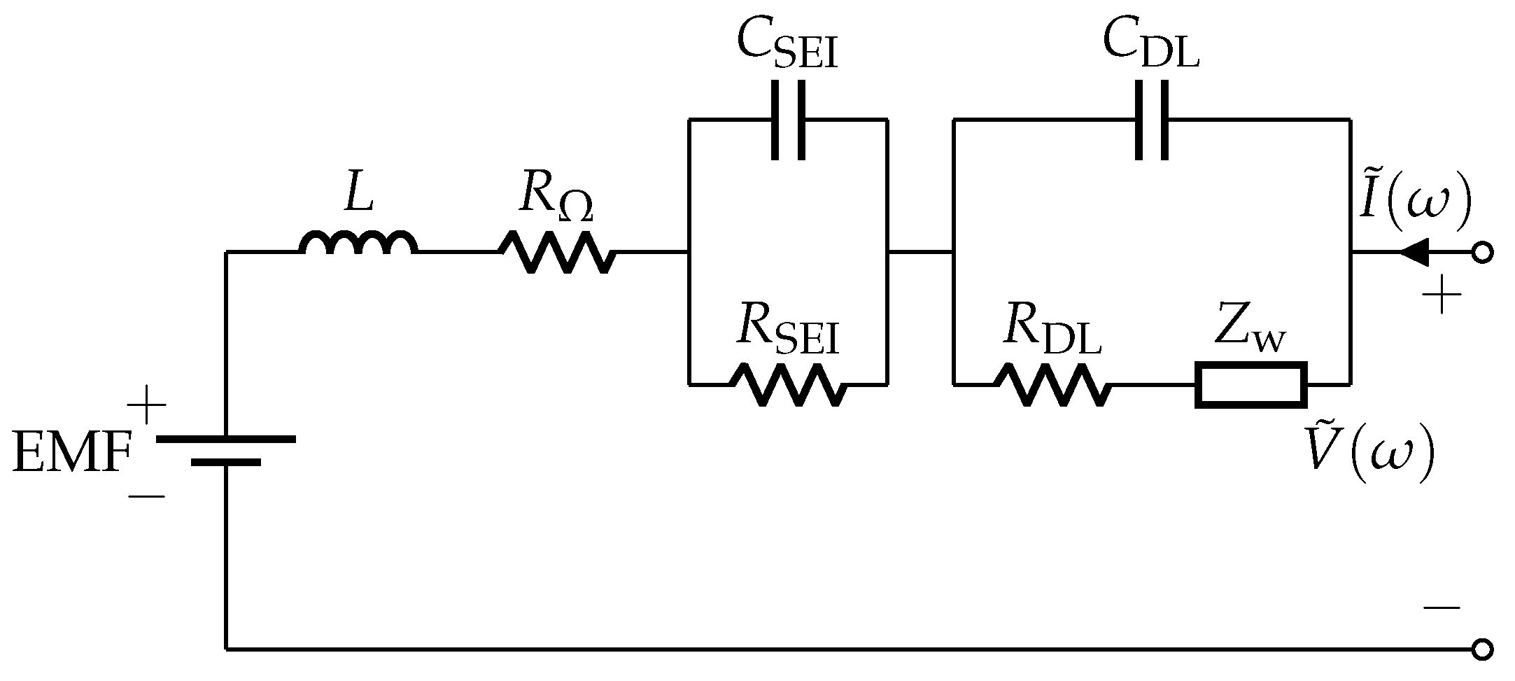
The frequency domain approach uses the Adaptive Randles equivalent circuit model (AR-ECM) shown in
Figure 1. The AR-ECM consists of the following elements: battery voltage source, ohmic resistance (
), stray inductance (L), resistance due to SEI layer (
), capacitance due to SEI layer (
), charge transfer resistance (
), double layer capacitance (
) and Warburg impedance (
). Figure 2.1(b) in [
27] shows the Nyquist plot relevant to the AR-ECM.
According to
Figure 1, the AC impedance
corresponding to AR-ECM can be written as [
27]
where
denotes the impedance in the RL arc,
denotes the impedance in the SEI arc, and
denotes the impedance in the CT arc and Diffusion arc.
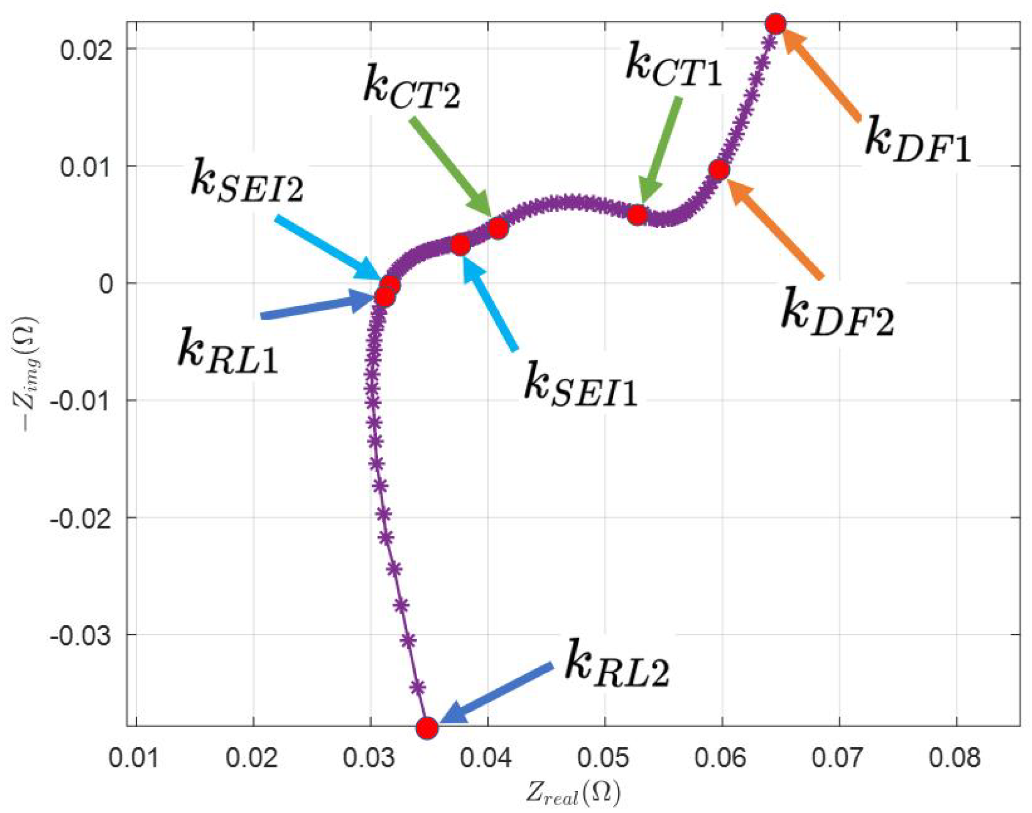
In
Figure 2, the feature points are selected manually, which are indicated by index
and
. From
Figure 1, it is clear that the measured Nyquist plot needs to be divided into several parts to see how it is directly related to the AR-ECM. Different parts of the Nyquist plot represent the battery’s impedance at different frequencies.
is the index of the first data point, that is, .
is selected such that the data points from to follow the linear line.
is selected at the beginning of the CT arc such that the data points start to follow the arc.
is selected at the end of CT arc such that to follows the CT arc to achieve the best fit.
Similarly, is selected at the beginning of the SEI arc.
is selected at the end of the SEI arc such that follow the SEI arc to achieve the best fit.
is selected at the beginning of the RL arc.
is selected at the end of the RL arc.
To solve the problem of ECM parameter estimation, using the least squares (LS) algorithm to fit the real Nyquist plot as shown in
Figure 2 is a promising approach, as this can reduce the effect of measurement noise to increase the accuracy of estimated parameters. The following section will summarize the LS approach [
27] to ECM parameters estimation based on the manually selected feature points.
2.1. Estimation of Ohmic Resistance and Stray Inductance
From the previous work in [
27], ohmic resistance
can be estimated as
and stray inductance
L can be estimated as
where
and
, and
.
2.2. Estimation of Warburg Coefficient
Warburg impedance is defined mathematically as
where
is the Warburg coefficient.
From
Figure 1, it is clear that the Warburg impedance is significant only at lower frequencies (
). In
Figure 2, feature points from
to
are selected (where
= 1), considering the real part of the impedance
in the diffusion arc:
where
. The expression
is used to reduce the effect of noise in the measurements.
The observation model corresponding to (
5) is
where
2.3. Estimation of and
The impedance for frequencies
is in a practical Nyquist plot as shown in
Figure 2; to fit the SEI arc precisely, we select feature points that lie between
and
. Therefore, the impedance of the SEI arc between
is given as
The impedance measurements in the SEI arc can be denoted as:
where
and
.
Estimation of the SEI arc is essentially the problem of fitting a semicircle with its center lying on the real axis; the coordinates of this semicircle’s center can be noted as (
, 0); the radius of the semicircle can be noted as
; therefore, the measurements in (
9) should satisfy the equation of the semicircle, which are given by
Let
and
, thus
In addition, (
11) can be rewritten as
In the matrix form, (
14) can be written as
Using the LS algorithm, the estimate of
will be given by
The estimates of
c and
d are:
From Figure 2.1(b) in [
27], the solid electrolyte interface resistance
is the diameter of the SEI arc; thus, by substituting the values of
c and
d in (
13), the estimate of
is
In (
1), when the frequency is very high, we assume the impedance in the CT arc and Diffusion arc will be very small so that it is negligible; thus, the
term will become zero, that is
Therefore, the impedance in the SEI arc can be expressed as:
Taking the imaginary part on both sides of the above equation,
Substituting the expression for
,
, and
L from (
18), (
2), and (
3), respectively, in (
24) at
:
Finally, we average all the estimates
to obtain the final estimate
2.4. Estimation of and
The practical Nyquist plot is shown in
Figure 2; to fit the CT arc precisely, we select feature points that lie between
and
; therefore, the impedance of the CT arc between
is given as
The impedance measurements in the CT arc can be denoted as:
where
and
.
Similar to the estimation of
,
can be estimated by fitting a semicircle to the CT arc. Assuming that the center of the semicircle lies on the real axis, which is noted as (
, 0), the radius of the semicircle can be noted as
; therefore, the measurements in (
28) should satisfy the equation of the semicircle, which is given by
Let
and
; thus,
Now, (
30) can be rewritten as
In the matrix form, (
33) can be written as
From (
34),
can be estimated using the LS algorithm
Thus, the estimates of a and b are:
From Figure 2.1(b) in [
27], the charge transfer resistance
is the diameter of the CT arc; thus, by substituting the values of
a and
b in (
32), the estimate of
is
Therefore, the impedance in the CT arc and Diffusion arc can be expressed as:
Taking the imaginary part on both sides of the above equation, and substituting
with the expression given in (
5), we obtain
Substituting
L,
,
,
,
and
with the estimations given in (
3), (
2), (
18), (
26), (
37), and (
7), respectively, in (
24) at
:
Finally, we average all the estimates
to obtain the final estimate
3. Time Domain Approach to ECM Parameter Estimation
Time domain approaches are widely used to estimate the internal resistance of the battery. Due to requiring less time consumption for its implementation, this approach is more suitable for real-time applications [
7,
8,
29]. One of the methods is to use the pulse stream current profile [
28], as shown in
Figure 3, to estimate the internal resistance of the battery.
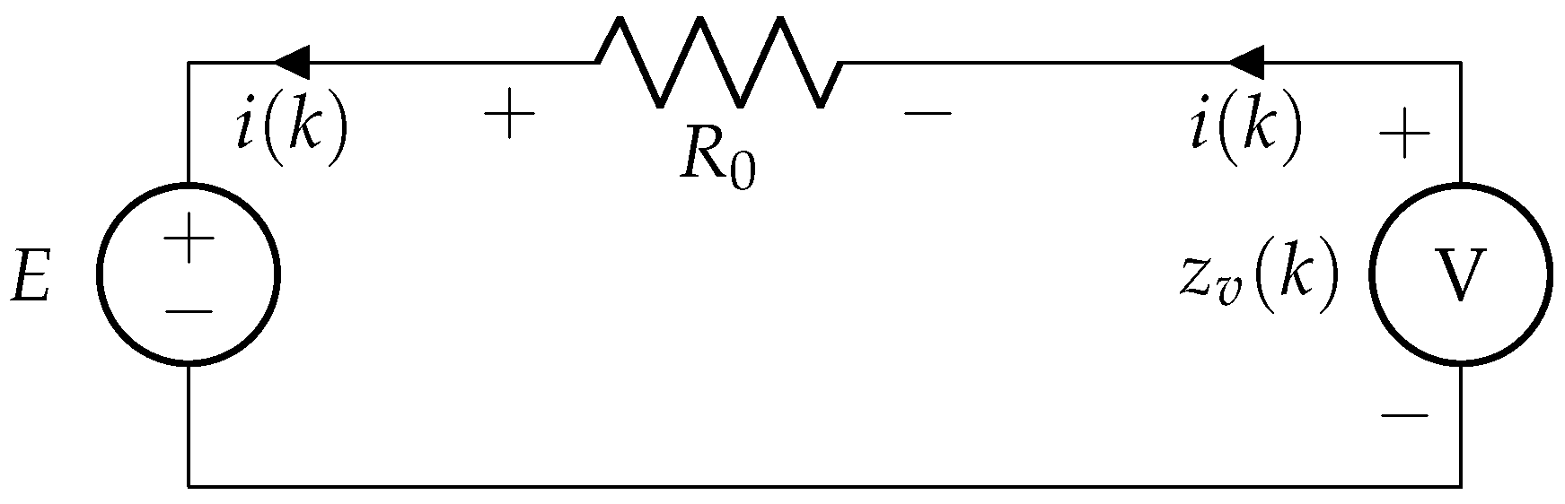
In
Figure 4, considering a simple R-int model: when current
is supplied to the battery, voltage
across its terminal is given by
where
E denotes the open circuit voltage, and
is the internal resistance of the battery.
Considering the presence of noise in measured voltage
, (
46) can be rewritten as
Assuming there are
n measurements in (
47), the following can be written
Equation (
48) can be written in the matrix form
E and
can be estimated using the LS approach:
4. Experimental Procedure
This section explains the experimental procedure for data collection. The specifications of LG and Molicel batteries are shown in
Table 1; four LG batteries are labeled as LG01, LG02, LG03, and LG04; and four Molicel batteries are labeled as MCL01, MCL02, MCL03, and MCL04. The data are collected using the Arbin battery cycler (Model: LBT21084UC). The Arbin cycler has 16 channels that can operate in parallel; eight channels were used to collect data simultaneously at room temperature (23
C).
The EIS data are collected by the EIS device (Gamry interface 5000P). A Gamry EIS device and Arbin battery cycler are operated using the software named Mits Pro provided by Arbin. The voltage measurement error of the Gamry EIS device, as specified, is 0.2 mV [
31].
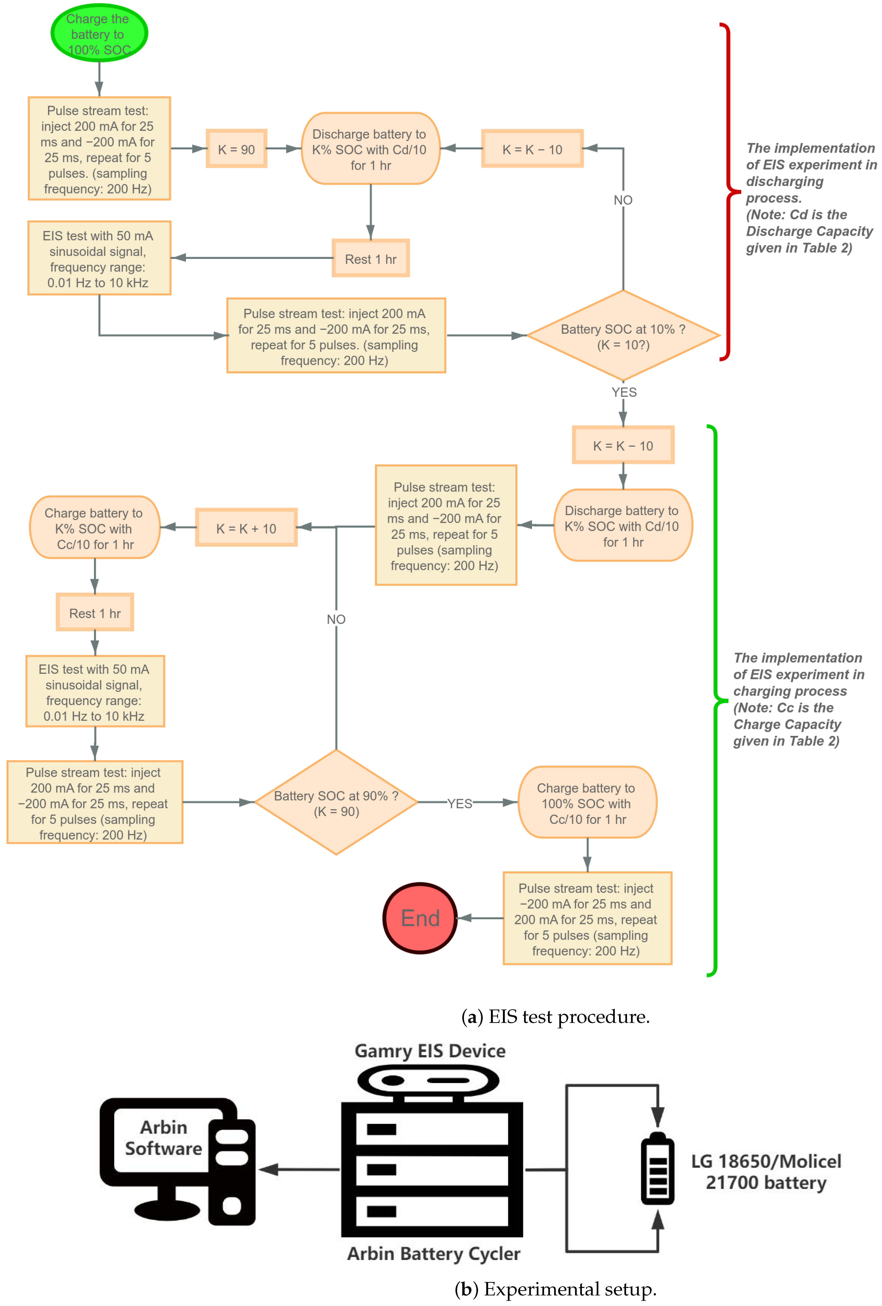
All experiments presented in this paper started with a fully charged battery (SOC = 100%) and the SOC is reduced by 10% at a time until the SOC reached 0%; after that, the SOC is increased by 10% at a time until the SOC returned to 100%. In this paper, discharging the battery with
A constant current or charging the battery with
A constant current for 1 h will decrease/increase the SOC by
; here,
is the discharge capacity and
is the charge capacity of the battery, which are given in
Table 2.
At each of these SOC levels except for
and
, an EIS experiment is performed; additionally, a time-domain experiment is also performed. For the time-domain experiment, the current profile detailed in
Figure 3 is applied right after the EIS experiment is conducted at the corresponding SOC. The detailed procedure is shown as follows:
OCV Test
- –
Figure 5 shows the detailed test procedure.
- –
Table 2 shows the actual discharge and charge capacity of the LG batteries and Molicel batteries, which are computed after the OCV test.
EIS Test
- –
The experimental procedure is shown in
Figure 6a.
- –
The experimental setup is shown in
Figure 6b.
5. Results
In this section, the results obtained from the experiment are shown and discussed.
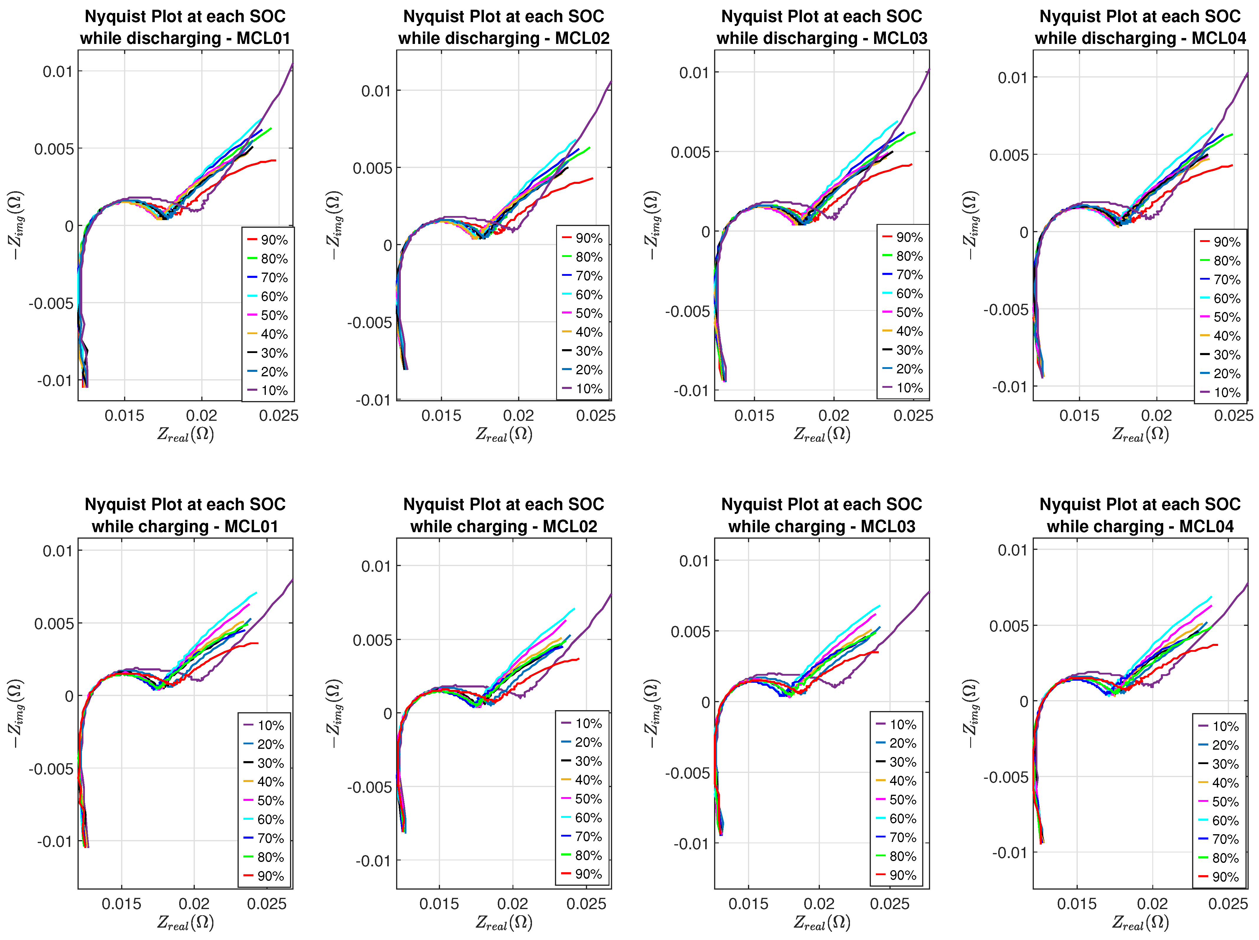
Nyquist plots of eight batteries at different SOC levels are shown in
Figure 7 and
Figure 8, where the SEI effect can be seen clearly in the Nyquist plot corresponding to 10% SOC while batteries are in the discharging or charging process.
In
Table 3,
Table 4,
Table 5 and
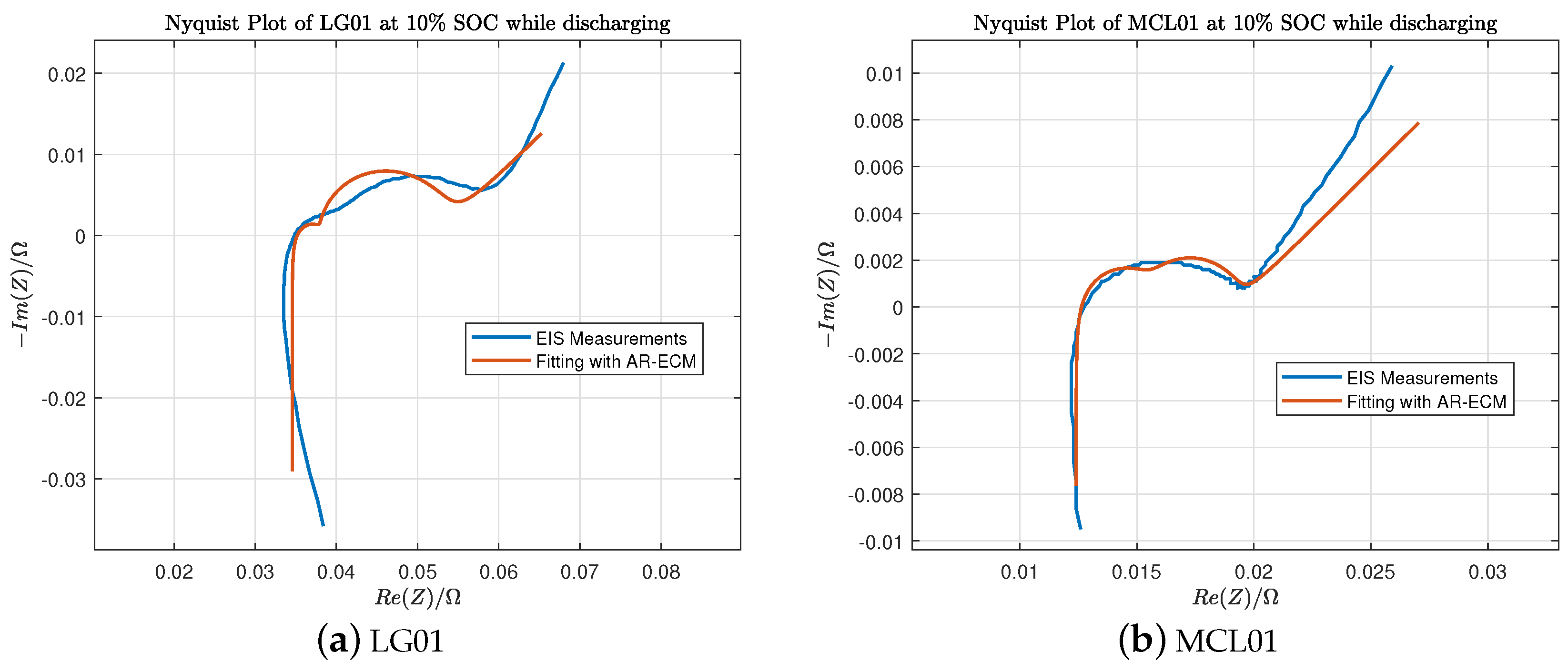
Table 6, the estimated ECM parameters for LG and Molicel batteries are obtained using the algorithms explained in
Section 2. We can observe that the internal resistance
measured by Arbin is quite close to the ohmic resistance
. Furthermore,
Figure 9a shows the fitted Nyquist plot of LG01 battery at
SOC while discharging, and
Figure 9b shows the fitted Nyquist plot of MCL01 battery at
SOC while discharging.
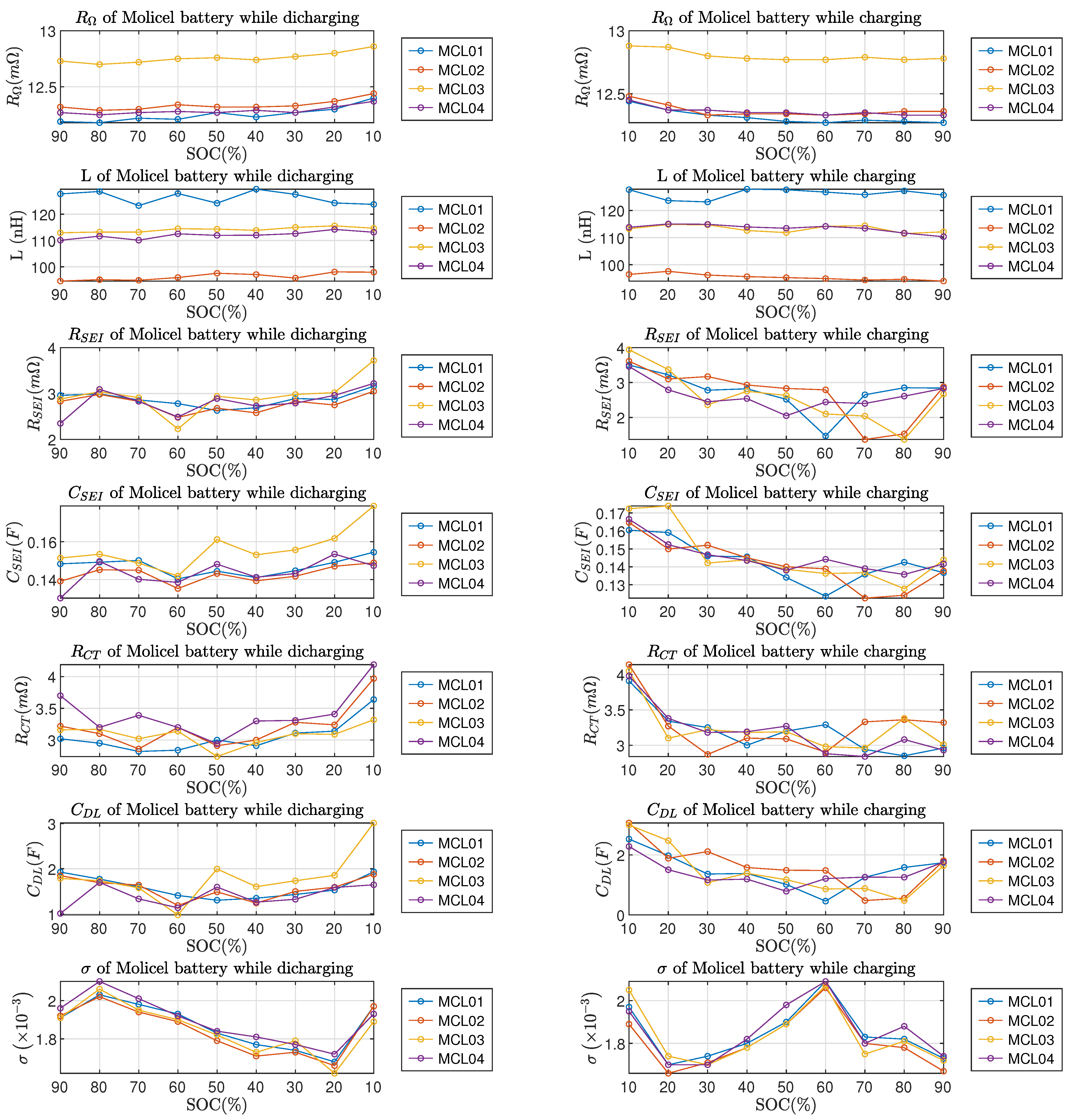
From
Figure 10 and
Figure 11, it can be observed that the ohmic resistance
, charge transfer resistance
and double-layer capacitance
all reached the highest value at
SOC; this phenomenon applies to both LG and Molicel batteries. The Warburg coefficient
of LG batteries reached the highest value at
SOC; as for Molicel batteries, the highest
occured at
while discharging and
while charging. In addition, no regularity can be found in LG and Molicel batteries with respect to the variations of
L,
and
at the
SOC level; also, the variations of all ECM parameters between
and
SOC are not significant in general.
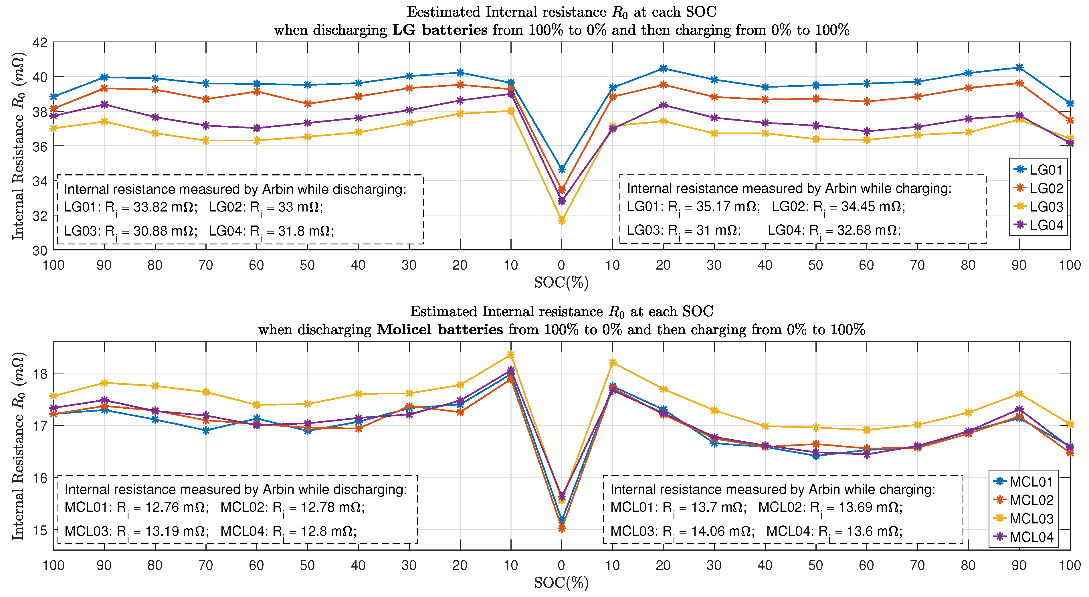
Figure 12 shows all the estimated internal resistance
using the time domain approaches presented in
Section 3. It can be seen that at
, both LG and Molicel batteries’ internal resistance
declined to the lowest value, whereas at
SOC, all the Molicel batteries’ internal resistance
reached the highest value.
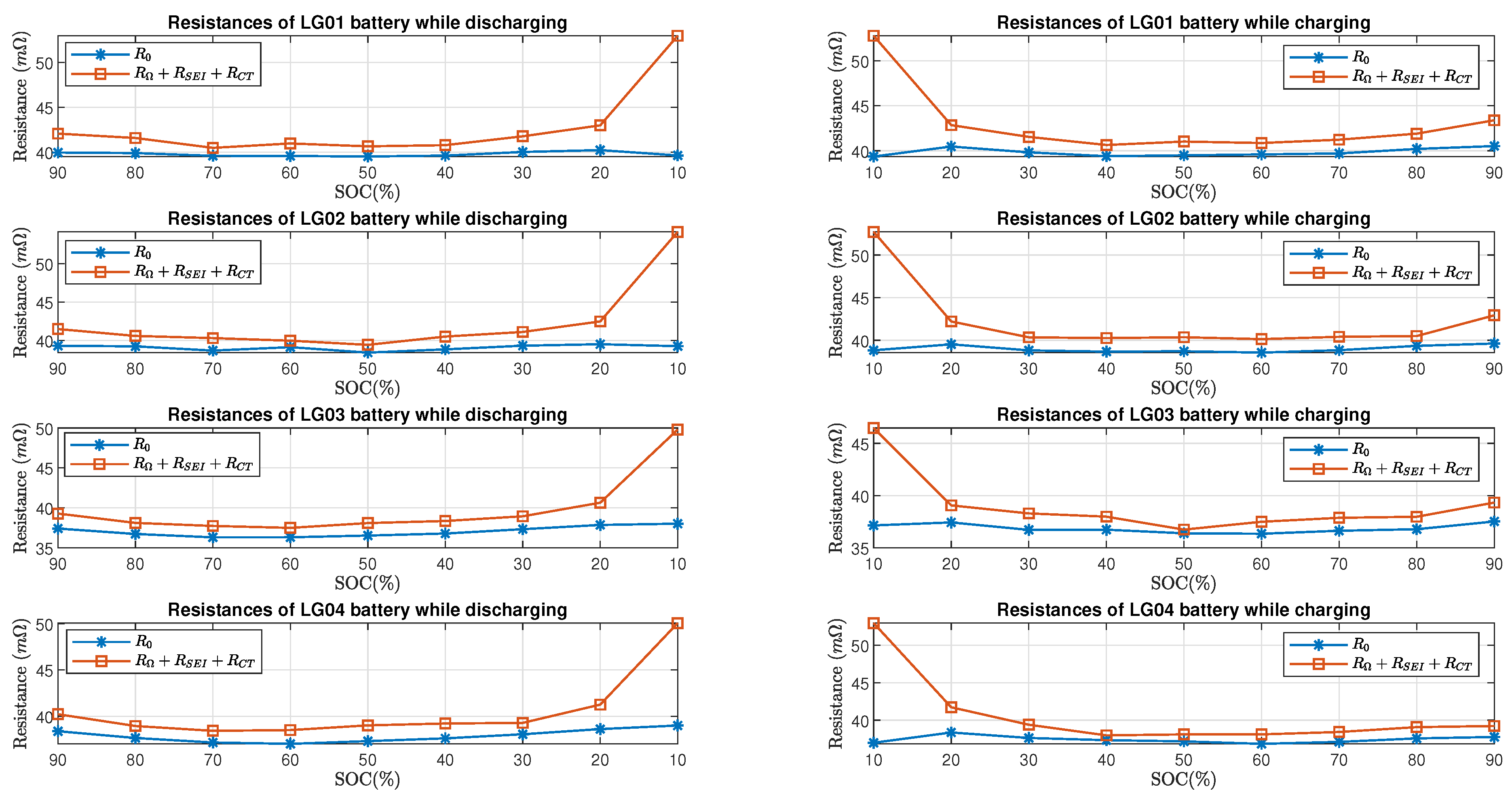
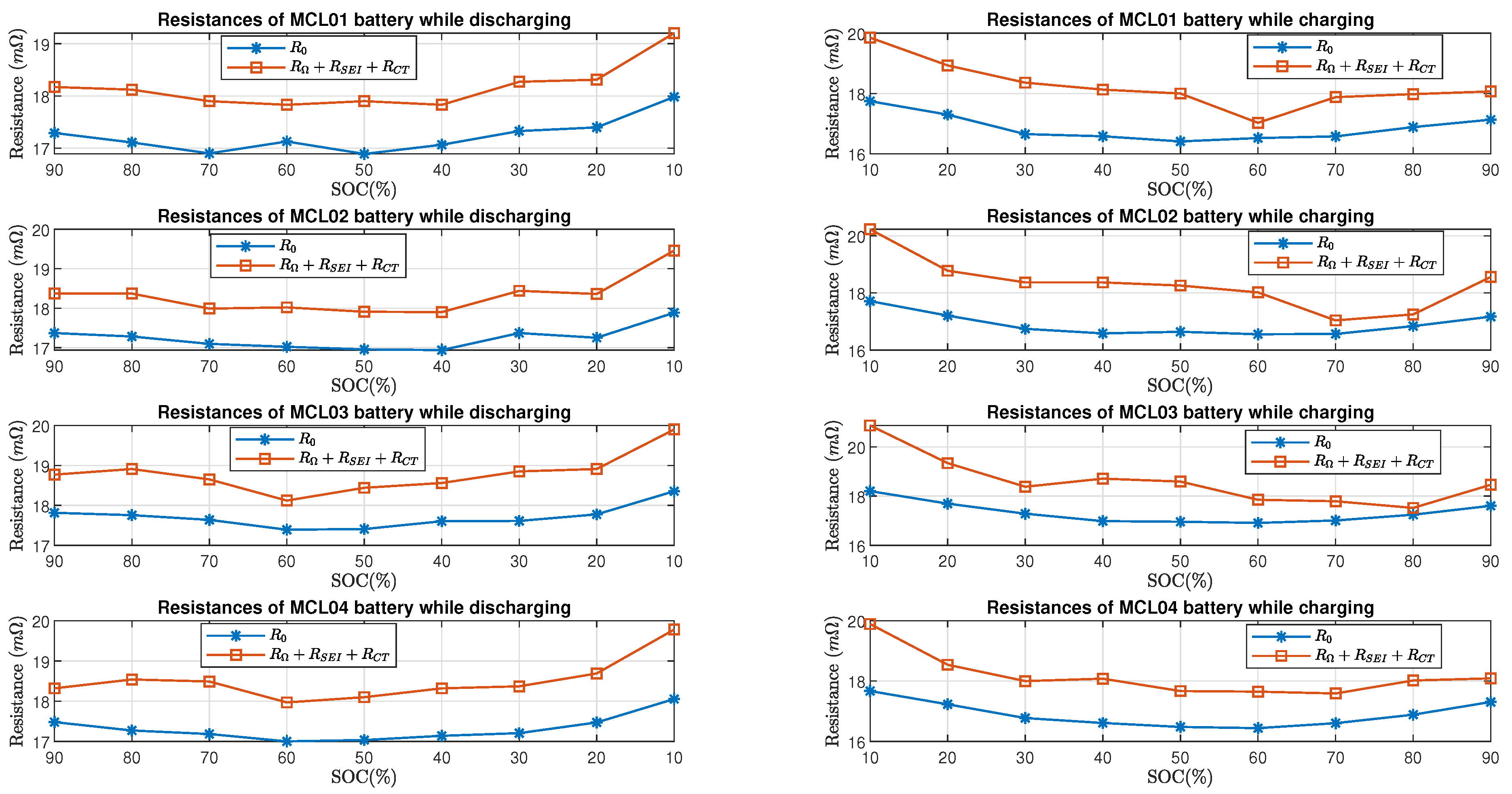
Figure 13 and
Figure 14 show the comparison of estimated total resistance
and the estimated internal resistance
of LG batteries and Molicel batteries, respectively. As for LG and Molicel batteries,
is slightly higher than
at all SOC, and it reached the highest value at
SOC.
Furthermore,
Figure 15 shows the percent error of the estimated resistive elements
with respect to the internal resistance
in the charging and discharging process. As for LG batteries, it can be seen that the percent errors are within
when the batteries’ SOC is between
and
while charging or discharging; at
SOC, the percent errors are between
and
in the discharging process, and they are between
and
in the charging process. As for Molicel batteries, when the SOC is between
and
, the percentage errors are within
while discharging and are within
while charging; at
SOC, the percentage errors are between
and
in the discharging process, and they are between
and
in the charging process.
6. Conclusions and Discussions
This paper demonstrates the parameter estimation to identify the resistive and inductive components in an AR-ECM based on the battery’s EIS.
The ECM parameter estimation approach is applied to the EIS data collected from LG 16850 and Molicel 21700 batteries at multiple SOC levels. The proposed approach is implemented via the manual selection of feature points from actual Nyquist plot; this relies on the precise separation of SEI arc, CT arc, and Diffusion arc from the real Nyquist plot, which has a low signal-to-noise ratio.
From the experiment, it is clear that the internal resistance measured by Arbin is actually the ohmic resistance from the AR-ECM; besides, whether it is an LG or Molicel battery, the variation of all estimated ECM parameters is very small when the SOC ranges from to ; furthermore; , and reached the highest value at SOC, whereas the variation of L, , and show irregularity at SOC; moreover, the total resistance reaches the highest value at SOC.
In addition, a time domain approach is developed to check the validity of the estimated ECM parameters; the validation is performed by using data collected from eight different batteries at nine different SOC levels both in the discharging and charging process, which shows good agreement between the time domain and frequency domain approaches when the battery’s SOC is between and . It must be noted that this approach is well suited to estimate resistive components only. When the RC effect increases, the accuracy of resistance estimation is expected to drop. The prominent error observed at SOC is due to the significant RC effect; this makes sense, since there are two RC elements in the AR-ECM. As a result, it can be concluded that there exists an inadequacy in the time domain approach for modeling all resistive elements at low SOC.
In future works, the automatic detection of feature points will be developed to improve the efficiency of ECM parameter estimation. Another limitation of the present work is that all the experiments were conducted at room temperature. Future studies will repeat these experiments at various temperatures to investigate whether the variation of temperature has an impact on ECM parameters.


