Article

Based on Improved NSGA-II Algorithm for Solving Time-Dependent Green Vehicle Routing Problem of Urban Waste Removal with the Consideration of Traffic Congestion: A Case Study in China

School of Management Science and Engineering, Anhui University of Technology, Ma’anshan 243002, China
*
Author to whom correspondence should be addressed.
Systems 2023, 11(4), 173; https://doi.org/10.3390/systems11040173
Submission received: 27 February 2023 / Revised: 24 March 2023 / Accepted: 24 March 2023 / Published: 27 March 2023
(This article belongs to the Topic Data-Driven Group Decision-Making)

Abstract

:
The dense population and the large amount of domestic waste generated make it difficult to determine the best route and departure time for waste removal trucks in a city. Aiming at the problems of municipal solid waste (MSW) removal and transportation not in time, high collection and transportation costs and high carbon emissions, this paper studies the vehicle routing problem of municipal solid waste removal under the influence of time-dependent travel time, traffic congestion and carbon emissions. In this paper, a dual objective model with the lowest total economic cost and the highest garbage removal efficiency is established, and a DCD-DE-NSGAII algorithm based on Dynamic Crowding Distance and Differential Evolution is designed to improve the search ability, improve the convergence speed and increase the diversity of the optimal solution set. The results show that: according to the actual situation of garbage collection and transportation, the method can scientifically plan the garbage collection and transportation route, give a reasonable garbage collection scheme and departure time, and effectively avoid traffic congestion time; Through algorithm comparison, the algorithm and model proposed in this paper can reduce collection and transportation costs, improve transportation efficiency and reduce environmental pollution.

1. Introduction

With the expansion of urban scale and the continuous improvement of residents’ consumption level, the production of municipal solid waste (MSW) is growing rapidly, and the problem of MSW is becoming more and more serious. Untimely garbage collection and transportation, high cost of garbage collection and transportation and high carbon emissions will bring a series of problems to society, economy and environment, which will greatly affect the development of a city. Because of it is particularly important to establish a reasonable vehicle scheduling model for MSW collection and transportation, and give a scientific and reasonable waste collection route, garbage collection schemes and vehicle departure time schemes.

1.1. Related work

1.1.1. VRP

Waste Collection vehicle routing problem (WC-VRP) is essentially a VRP, but it is different from the traditional VRP. It needs to consider more constraints and factors, such as time window constraints, vehicle capacity constraints, various vehicle types, garbage station capacity constraints, nodes need to be accessed by multiple vehicles, traffic congestion, and special conditions of road networks caused by weather changes. Aiming at the problem of garbage collection vehicle routing in different situations, scholars in domestic and foreign have conducted a series of studies. Molina et al. [1] changed the economically focused objective of the traditional waste removal vehicle path problem, which does not take into account the importance of the environment. A model with ecological efficiency as the goal was proposed and solved it using a variable neighborhood forbidden search algorithm, which was validated on a real problem in the city of Guadaira, within the Seville (Spain) metropolitan area. Nurprihatin et al. [2] considered the constraints of split delivery, multiple trips, time windows, and different vehicle types, and established a WC-VRP model with the minimum total cost and travel distance as the optimization goal. Farrokhi-Asl et al. [3] established a social and economic dual-objective garbage collection model with time window constraint, solved it by NSGA-II algorithm and MOPSO algorithm respectively, and proved that NSGA-II algorithm can obtain better results. Rabani et al. [4] considered different vehicle types, time window constraints, vehicle capacity constraints and site capacity constraints, and established a model with the lowest transportation cost, the smallest number of vehicles used and the minimum number of disposal centers. Hina et al. [5] proposed a two-city garbage collection vehicle path planning method, which considers regional constraints, vehicle capacity and time window constraints, and established a model aiming at the minimum vehicle driving distance. The model provides a decision-making basis for municipal management departments to effectively clear and transport solid waste. Ahlaqqach et al. [6] established a VRP model for medical waste removal, considering the heterogeneity of vehicles, the risk of waste collection and time window constraints, and solve it with a genetic algorithm. Dereci et al. [7] considered both solid waste optimization and VRP to solve the route optimization problem with multiple heuristic and meta-heuristic algorithms with the objective of solid waste collection route optimization in Istanbul Umraniye district.

1.1.2. GVRP

Through the above literature on garbage removal vehicle routing, it is found that most studies only consider economic factors, rarely consider environmental factors, and there is a lack of research on carbon emissions calculation methods. Therefore, this paper considers the factor of carbon emissions in the model construction, and at the same time, a large number of domestic and foreign research on green vehicle routing problem (GVRP). Niu et al. [8] proposed a formula to calculate carbon emissions, and modeled it with the goal of minimum cost of carbon emissions, fuel consumption and driver’s salary. Rauniyar et al. [9] constructed a GVRP model with the goal of minimizing the total cost and total travel distance with capacity constraints, and solve it by genetic algorithm. Qiu et al. [10] established and solved a multi-objective green vehicle routing model with the goal of minimizing fuel consumption, penalty cost and distribution income variance. Zhou Guo et al. [11] constructed a mathematical optimization model for the GVRP of multi-to-many cross-docking distribution with the goal of minimizing the sum of vehicle operation cost, carbon emission cost and fuel consumption cost. Zhou et al. [12] and Erdoğdu et al. [13] established the dual-objective GVRP and designed algorithms to solve it.

1.1.3. TDGVRP

Most of the above research results focus on the GVRP with constant vehicle speed, but the variability of vehicle speed needs to be considered in the actual traffic network. Soysal [14] and Cimen [15] expressed the time-dependent GVRP (TDGVRP) of variable speed as a Markov decision process and solved it by dynamic programming. Considering the effects of time-dependent speed and carbon emissions and load on vehicle fuel consumption, Zhou et al. [16,17] constructed a multi-objective TDGVRP model and designed an improved ant colony algorithm to solve it. Ge Xianlong et al. [18] considered the factor of time-dependent traffic congestion, established a dual-objective model with minimum carbon emissions and minimum travel time, and solved it with an improved tabu search algorithm. Chen Cheng et al. [19] studied the VRP of city distribution based on the spatiotemporal dynamics of speed, and incorporated the carbon emissions cost into the model, and solved it by the variable neighborhood search algorithm. Zhu Lan et al. [20] proposed a time-dependent green vehicle routing model to reduce transportation costs and environmental pollution by optimizing transportation routes and departure times. Luo et al. [21] considered the TDGVRP with traffic congestion, developed a set partition formulation (SPF), and proposed a branch-price-and-cut (BPC) algorithm to solve it. Liu et al. [22] studied the time-dependent GVRP with time windows (TDGVRPTW) considering time-dependent travel times and time window constraints and integrating the minimization of carbon emissions, and designed an efficient adaptive large neighborhood search (ALNS) algorithm to solve it.

1.1.4. Non-Dominated Sorting Genetic Algorithm

The Non-Dominated Sorting Genetic Algorithm (NSGA-II) based Genetic Algorithm (GA) can be used to solve multi-objective optimization problems and was originally proposed by Deb et al. in 2000 [23] and the complete research article was published in 2002 [24]. In the review of NSGA-II, Verma et al. [25] summarized the application of NSGA-II and its variants in specific Combinatorial Optimization Problems (COPS), such as assignment problem, traveling salesman problem, vehicle routing problem (VRP) and scheduling problem, etc. The following article briefly introduces the application of NSGA-II in VRP. Xu et al. [26] introduced a hybrid algorithm involving NSGA-II and Or-opt heuristic to solve a multi-objective model for VRPTW. Liu et al. [27] proposed a four-objective dynamic routing planning problem to achieve simpler routing and better user experience, and designed and used the NSGA-II node-based crossover operator to solve the proposed model. Wang Y et al. [28] combined k-means and NSGA-II to propose a hybrid heuristic algorithm (HNSGA-II) for solving the collaborative multiple centers vehicle routing problem with simultaneous delivery and pickup (CMCVRPSDP), and compared it with the traditional NSGA-II and Multi-Objective Particle Swarm Optimization (MOPSO) algorithms, and the results showed that HNSGA-II has better performance in objective function values. Srivastava et al. [29] proposed a NSGA-II based algorithm to solve VRPTW with five generic objectives, and the results showed the superiority of this algorithm compared to previous methods.

1.2. Our Contributions and Overview of the Paper

In summary, the existing results have laid a good theoretical foundation for further research on the routing problem of MSW removal, but there are still research gaps as follows: (1) Most of the studies are on single vehicle types, and there are fewer studies on multi-vehicle cases. (2) Vehicles visit each node only once, and there is a lack of studies on nodes visited by multiple vehicles. (3) When studying the effects of different vehicle speeds on path planning in time-dependent road networks, most assume that vehicles start at the same moment, and there is a relative lack of research results on vehicles starting from different times to avoid traffic congestion.
The purpose of this study is to find the best route and vehicle start time to meet the demand by considering the MSW collection process in Ma’anshan City. All data used in this paper were obtained from the Environmental Health Management Department of Ma’anshan City. The contributions of this paper are summarized as follows:
  • In this paper, we introduce traffic congestion coefficients to simulate the congestion level of roads at different time periods, and consider constraints such as multiple vehicle types, multiple vehicle visits, different vehicle departure moments, and time windows to construct and solve a multi-objective model with minimum total economic cost and minimum total timeout. The traditional NSGA-II algorithm search weak search capability and poor convergence in solving multi-objectives, so we design a DCD-DE-NSGAII algorithm based on Dynamic Crowding Distance and Differential Evolution;
  • The model and the proposed algorithm can give reasonable vehicle scheduling scheme according to the preference of decision maker, which can provide solutions and suggestions for government departments to solve the problems of untimely urban waste removal and high cost of collection and transportation.
The remain of the paper is organized as follows. Section 2 describes the main research problem and model of this paper. Section 3 describes the DCD-DE-NSGAII algorithm in detail. Section 4 reports the data analysis of the examples in the literature. Section 5 summarizes the research and discusses future research directions.

2. Problem and Model

2.1. Problem Description

This paper investigates the specific situation of garbage removal in Ma’anshan City, and the actual situation of waste removal vehicle dispatching in Ma’anshan City was modeled. The problem is described as follows: the garbage trucks (all garbage trucks are parked at the City Administration) are uniformly sent by the sanitation department of the City Administration to collect garbage at various waste transfer stations and transported it to Xiangshan waste incineration plant. After the garbage trucks are transported to the waste incineration plant, they return to the city center to continue collecting and transporting garbage (do not return to the City Administration), and then to Xiangshan waste incineration plant until the day’s cleaning and transportation task is completed. The location of each garbage transfer station and the amount of garbage are known, and the driving speed of vehicles in different time periods is affected by traffic conditions. The optimization model is to establish with the objective of lowest the total cost and total timeout (the sum of the time when the moment of completion of each garbage station’s removal exceeds the latest time window specified for that garbage station). To further clarify the research of this scope of this paper, the following hypotheses are proposed.
(1)
The garbage truck has two types of heavy load (maximum load: 8 tons) and light duty (maximum load: 5 tons). There are 45 garbage trucks in total in the City Administration Environmental Sanitation Department. All garbage trucks must return to the Sanitation Department before 18:00;
(2)
According to the actual needs, different vehicles can set off at different times, but it must be ensured that a garbage truck is sent out at 5: 30 am, and the rest of the garbage trucks can be sent out in succession;
(3)
The vehicle runs at a normal speed during the normal driving period, and runs at a congestion speed during the traffic congestion period;
(4)
For stations with a high volume of waste, determine which vehicles will be transported according to the nearest principle;
(5)
The amount of garbage loaded cannot exceed the maximum capacity of the vehicle, and if a garbage truck is not full at a transfer station, it can be judged according to the nearest principle whether the truck should go to the next transfer station to continue loading;
(6)
Each garbage transfer station has a service time window requirement. Each garbage transfer station does not have the earliest time window requirement, but has the latest time window requirement. The time for each garbage station to complete the day’s cleaning task exceeds its latest time window;
(7)
Not all of the 45 garbage trucks have to be sent out. If the car in front of them can ensure that the amount of garbage can be delivered for the day, stop the departure; the drivers of garbage trucks have a rest from 12:00–14:30 noon, and the drivers who arrive at the transfer station during this time will have a rest, and not carry out garbage transportation;
(8)
All garbage of all garbage transfer stations must be cleared daily;
(9)
The usage cost includes vehicle travel time cost, service time cost and fixed departure cost;
(10)
The service time for the vehicles to collect garbage at each transfer station is 10 min, and the time for the garbage trucks to reach the incineration plant to unload garbage is also 10 min. In addition, during the service period, the engine is closed without fuel consumption and carbon emissions;
(11)
Using multiple models for distribution, the weight, maximum load and fixed start-up cost of each model are different;
(12)
It is assumed that the daily traffic congestion time periods are 7:00–9:00 and 17:00–18:00 respectively, and the rest of the time periods are set as normal driving time periods.

2.2. Symbols and Variables

The meanings of variables, sets, and decision variables are shown in Table 1.

2.3. Mathematical Model

This model has two objective functions, the first objective is to minimize the sum of carbon emission cost, vehicle fuel consumption cost, driver’s wage cost and vehicle use cost, and the second is to minimize the total overtime time (to effectively quantify waste removal efficiency by total vehicle overtime time). A multi-objective, multi-vehicle VRP model with capacity constraints, time window constraints and multi-vehicle access considering the influence of time-dependent vehicle speed and carbon emissions are constructed, as follows:
m i n f 1 = C 1 + C 2 + C 3 + C 4
C 1 = h H i A j A k K F C i j k h C f Z i j k h
C 2 = h H i ϵ A j ϵ A k ϵ K E C i j k h C e Z i j k h
C 3 = h H i A j A k K μ t i j k h Z i j k h + h H i A μ s i h X i h + h H σ h ζ
C 4 = h H i A j A k K ψ t i j k h Z i j k h + h H i A ψ S i h X i h
m i n f 2 = s u m m a x A T i L T i , 0
s.t.
h H X i h 1 i N
y i j h Z i j k h , i , j A , k K , h H
y i j h k K Z i j k h , i , j A , h H
i N y i j h = j N y i j h , h H
d i j k h D i j Z i j k h , i , j A , k K , h H
k K h H d i j k h = D i j X i j , i , j A
β i h + S i h l i h , i A ,   h H
t i j h = k K t i j k h y i j h , i N ,   j N ,   h H
β j h = l i h + t i h
i P j P h H q i h y i j h H Q ,       h H
i P h H q i h X i h = Q i
h H σ h n q + n z
D i j 0 ,   Q i 0 ,   q i h 0 ,   H Q q 0 ,   H Q z 0 L T i 0 ,   A T i 0 ,   β i h 0 , l i h 0 ,   S i h 0 b k 0 , e k 0 , V i j k 0 ,   d i j k h 0 ,   t i j k h 0
X i h 0 , 1 ,   X i j 0 , 1 ,   σ h 0 , 1 y i j h 0 , 1 ,   Z i j k h 0 , 1
The objective function f 1 represents the minimum total economic cost of garbage removal, where C 1 represents the fuel consumption cost of garbage trucks, C 2 represents the carbon emissions cost, C 3 represents the use cost of garbage trucks, including vehicle driving time cost, vehicle garbage loading and unloading time cost and fixed departure cost, C 4 represents the driver’s wage cost; The objective function f 2 represents the minimum total timeout (the sum of time when each garbage station completes the cleaning task exceeds the latest time window of the garbage station); Equation (7) indicates that each transfer station can be served multiple times by the garbage truck; Equations (8) and (9) represents the restriction relationship between variables y i j h and Z i j k h ; Equation (10) ensures that the arrival and departure of the vehicle are the same demand point; Equation (11) represents the restriction relationship between variable d i j k h and D i j ; Equation (12) ensures that the vehicle will drive a complete road as long as the road is selected by the vehicle; Equation (13) represents the relationship between vehicle arrival time at the transit station, service time and departure time; Equation (14) represents the calculation of the full travel time of the vehicle on the road i , j ; Equation (15) represents the time connection relationship of vehicles driving on different road sections; Equation (16) represents the capacity constraint of the vehicle; Equation (17) means that the garbage of each site must be cleared; Equation (18) indicates that the number of vehicles used shall not be greater than the maximum number of vehicles in the sanitation department; Equations (19) and (20) represent variable value constraints.

2.4. Fuel Consumption and Carbon Emissions Calculation

In this paper, the CMEM (Comprehensive Modal Emission Model) proposed by Barth [30] is used to calculate the vehicle fuel consumption to make the calculation more realistic. If the driving distance of vehicle h on the road i , j in time period k is d i j k h , the calculation of vehicle fuel consumption is shown in Equation (21).
F C i j k h = α 1 d i j k h V i j k + α 2 d i j k h V i j k 2 + α 3 ω + f i j k h d i j k h
where, α 1 is the engine module coefficient, α 2 is the speed module coefficient, α 3 is the load module coefficient, ω is the vehicle dead weight (unit: kg), f i j k h is the load of vehicle h driving on road i , j in time period k (unit: kg). It has been shown in the literature that the relationship between the carbon emissions of a vehicle and the fuel consumption is positive, and the carbon emissions of a vehicle are calculated as shown in Equation (22).
E C i j k h = F E F C i j k h
where, F E is the fuel emission parameter, generally considered as a constant. In this paper, the value of F E is 2.621 kg/L.

2.5. Calculation of Vehicle Travel Time

In the traditional VRP, the vehicle speed is not time-dependent and runs at a constant speed. However, in the case of traffic congestion, the speed of the garbage truck is time-dependent, and the speed of the vehicle in different time periods is different. In particular, even if the vehicle is driving on the same road section, it may drive at normal speed during the normal driving period in part of the road section, and driving at normal speed during the congestion period in the rest of the road section. The driving time of the vehicle on the road section i , j is difficult to calculate directly and must be dealt with reasonably. Therefore, this paper adopts the method of Zhou X [17] based on road division to calculate the driving time of garbage truck. Due to the space problem, the specific calculation steps are not shown.

3. Solution Algorithm Design

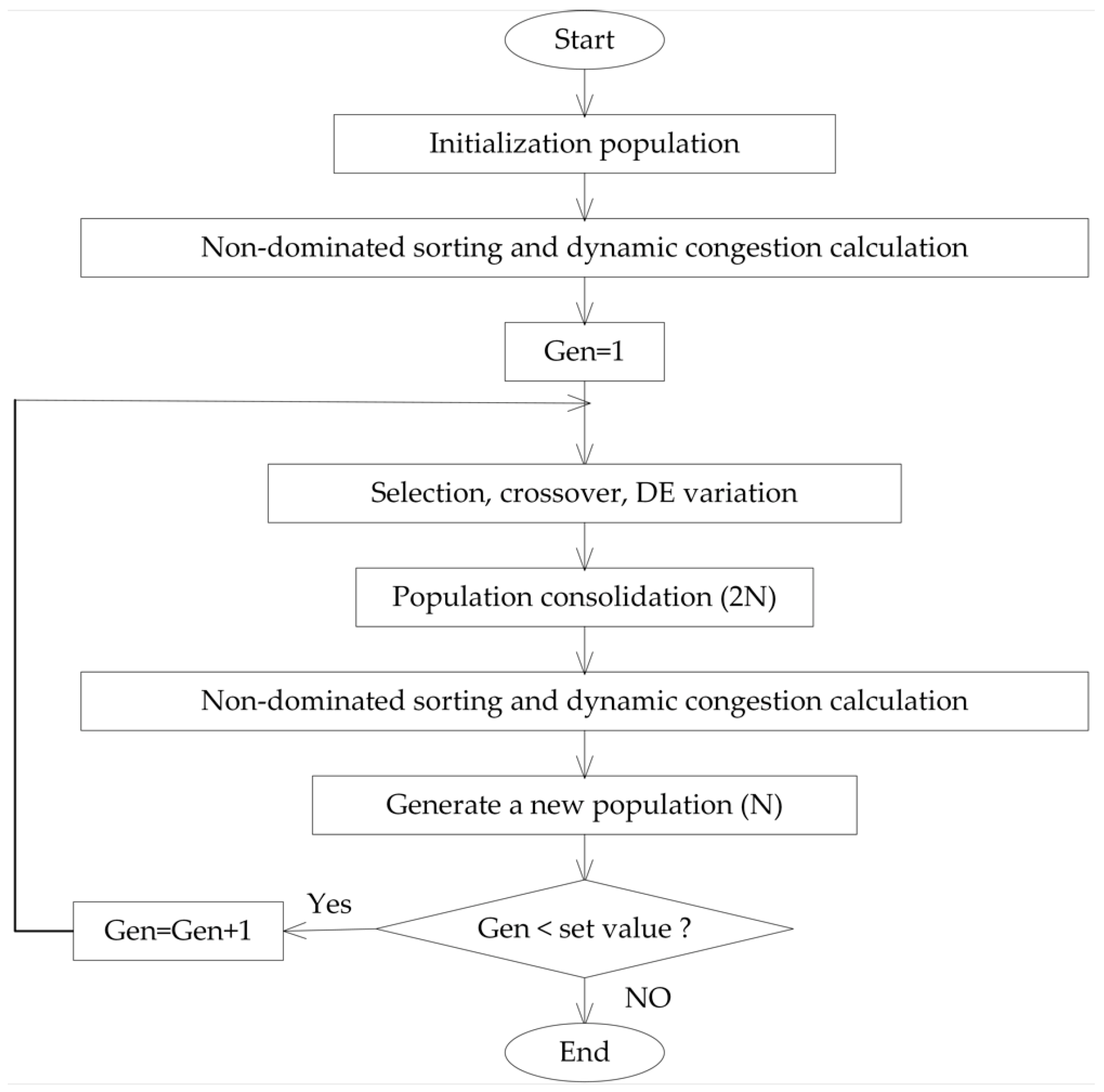
3.1. Improved DCD-DE-NSGAII Algorithm

The multi-objective optimization problem is usually solved using the NSGA-II algorithm, but the classical NSGA-II algorithm shows weak search ability and poor convergence when solving multi-objective problems. Therefore, this paper proposes a DCD-DE-NSGAII algorithm based on Dynamic Crowding Distance and Differential Evolution. The dynamic crowding sorting strategy [31] is used to overcome the defect of poor diversity of solution sets in traditional crowding sorting methods; to protect the population diversity and prevent premature, the polynomial mutation is replaced by differential mutation, and the scaling factor in differential mutation was improved; the probability of crossover and mutation is improved from a fixed value to decrease with the increase of the number of iterations according to the logsig function to effectively save the optimal gene and increase the possibility of searching the global optimal solution.
The specific improvements are described as follows:
(1)
Differential mutation operation [32]
The mutation operation is to homogenize the spatial distribution of the Pareto optimal solution to satisfy the population diversity. In the m th iteration, three individuals are randomly selected from the population. X p 1 m , X p 2 m , X p 3 m and p 1 p 2 p 3 i , i 1 , 2 , N . The vector formula of the generated mutant target individual is shown as follows:
F i m = X p 1 m + F · X p 2 m X p 3 m
where F is the scaling factor and the range of F is [0, 1].
(2)
Improvement of scaling factor [32]
As can be seen from Equation (23), parameter F is a fixed value randomly selected between [0, 1], and studies on its sensitivity are lacking. The generation of new individuals in the population mainly depends on the mutation operation, and the parameter F has a great influence on its search range. Furthermore, the convergence efficiency of the algorithm and the diversity of the solution range are further improved, and the parameter F is improved as follows:
F = F m i n + F m a x F m i n · e 1 m g m g m + 1
In the formula, F m a x and F m i n denote the minimum and maximum values of variation parameters, m represents the current number of iterations, and m g represents the maximum number of iterations. It can be seen from Equation (24) that with the increase of iteration times, the adaptive variation factor F m a x gradually decreases and becomes equal to F m i n , which can ensure the diversity of individual populations and avoid premature convergence:
(3)
Improvement of crossover and mutation probability
The cross-variance and mutation probability is no longer a fixed value, but decreases according to logsig function as the number of iterations increases.
Set the crossover probability to:
c p = 0.5 + 0.5 log s i g l i n s p a c e 3 , 3 , i t e r a t i o n s
Set the mutation probability to:
m p = 0.1 + 0.3 log s i g l i n s p a c e 3 , 3 , i t e r a t i o n s

3.2. Algorithmic Flow

The specific flowchart of the algorithm is shown in Figure 1 (which was created by the authors):

4. Case Analysis

4.1. Instance Data and Parameter Settings

In this paper, the specific situation of garbage removal in Ma’anshan City was investigated on the spot, and the location of each garbage transfer station, daily garbage output and other specific information were obtained from Ma’anshan City Administrative, as shown in Table 2 the specific information of the vehicle is shown in Table 3, and the other relevant parameter information of the model is shown in Table 4. In order to facilitate the simulation analysis, the time is unified from hours to minutes, for example, the earliest time of the vehicle at 5: 30 to 330 min.

4.2. Algorithm Performance Analysis

To test the performance of the DCD-DE-NSGAII algorithm, based on the experimental data of the actual example, the algorithm parameters are set as follows: The initial population size p o p s i z e = 20 , scaling factor F m i n = 1 ,   F m a x = 2 . Under the environment of 1.6 GHz IntelCorei5 processor and Win10 operating system, the DCD-DE-NSGAII algorithm and the NSGAII algorithm run 10 times respectively. The Pareto frontier comparison of the two algorithms is shown in Figure 2, the Pareto optimal solution is shown in Table 5, and the statistical results and the percentage of algorithm improvement are shown in Table 6 in Section 4.3.
In this paper, the improved DCD-DE-NSGA-II algorithm is analyzed with the classical NSGA-II algorithm. From the pareto frontier comparison diagram of the two algorithms in Figure 2, it can be seen that the DCD-DE-NSGA-II algorithm has more optimal solutions in the Pareto solution set, and the Pareto frontier has better distribution. DCD-DE-NSGAII obtains 13 Pareto solutions, while classical NSGAII only obtains 7 Pareto solutions. As can be seen from Table 5, in terms of total economic cost and total timeout time, the DCD-DE-NSGAII algorithm proposed in this paper embodies the advantages of differential variation and dynamic congestion, and has better solution quality.

4.3. Solution Result Analysis

The model established in this paper is solved using the proposed DCD-DE-NSGAII algorithm, and the extreme value solutions corresponding to different objective functions and various cost equivalents are obtained as shown in Table 6.
Table 6. Target values and costs.
f * Total Economic Cost/(Yuan)Total Timeout
/(min)
Fuel Consumption Cost/(Yuan)Carbon Emissions Cost/(Yuan)Vehicle Use Cost/(Yuan)Wage Cost/(Yuan)Carbon Emissions Ratio/(%)
f 1 * 25,940.00921.152945.40627.1018,425.003941.802.42
f 2 * 27,217.00615.163116.20663.4519,303.004134.502.44
Table 6 shows that when the government department prefers the optimal total economic cost, the corresponding total timeout time achieves a non-inferior solution, which is 49.74% higher than the minimum total timeout time. At this time, the carbon emissions cost, fuel consumption cost, use cost and driver’s wage cost of the vehicle are 2945.40 yuan, 627.10 yuan, 18,425 yuan and 3941.80 yuan respectively; When the government prefers the optimal total timeout, the corresponding total economic cost obtains a non-inferior solution, which increases by 4.92% compared with the minimum total economic cost. At this time, the fuel consumption cost, carbon emissions cost, use cost and driver’s wage cost of the vehicle are 31,116.2 yuan, 663.45 yuan, 19,303 yuan and 4134.5 yuan respectively.
Table 6 shows that whether the economic cost is optimal or the total overtime time is optimal, the cost of carbon emissions accounts for no more than 3% of the total cost, but the cost of vehicle usage accounts for a large proportion, reaching more than 70%. Therefore, to reduce the total economic cost, government departments should focus on reducing the cost of vehicle use, reducing the use of vehicles and shortening the total service time of vehicles on the basis of ensuring that the amount of garbage can be disposed of on the day, so as to minimize the total economic cost and reduce expenses.

4.4. Solution Analysis

Table 7 shows the final vehicle path scheduling scheme that the program derives when the government decision maker prefers the optimal total economic cost; Table 8 shows the optimized vehicle removal time corresponding to the vehicle path scheduling scheme; Table 9 shows the vehicle waste load at each station corresponding to the vehicle path scheduling scheme.
It can be seen from Table 7 that: 1. Although the Urban Authority has 45 garbage trucks, in fact only 30 are used. This program greatly reduces the use of garbage trucks and saves costs and financial expenses to a large extent. 2. The scheme put all the heavy-duty garbage trucks (8 in total) into use, and 22 light-duty garbage trucks were used. In reality, government departments use heavy-duty garbage trucks as much as possible to improve the efficiency of cleaning and transportation. 3. From the results of vehicle scheduling path, the total number of departures is 103 times, in the actual situation, the government departments may be more than 120 times a day, which can be compared to the scheduling scheme of this paper can effectively reduce the number of departures.
Table 8 shows the time when the garbage truck arrives at each station corresponding to the path plan of each vehicle in the table. From the distribution of garbage removal time, it can be seen that: 1. A total of 21 garbage trucks were sent out in the morning and 9 in the afternoon. Among the 30 garbage trucks sent out, the latest time to return to the City Administrative is 969.31, and 30 garbage trucks were guaranteed to return to the City Administrative parking lot before 18:00 at night. 2. Among the 30 garbage trucks issued, only the first 14 entered the 7:00–9:00 morning peak congestion period, but avoided the 17:00–18:00 evening peak congestion period, and the remaining 16 garbage trucks could avoid both periods. If according to the traditional vehicle routing problem, all vehicles start from the same time, all vehicles cannot avoid the morning congestion period. This shows that the model and the improved DCD-DE-NSGAII algorithm constructed in this paper can reasonably optimize the vehicle clearance time according to the time window characteristics of each garbage station, effectively avoid the traffic congestion period, and improve the efficiency of garbage clearance.
Similarly, when the government decision makers prefer the optimal total timeout time, the corresponding vehicle routing scheduling scheme table, vehicle clearance time optimization table, will also be obtained. Due to the length problem, it will not be displayed. Table 9 gives the comparison of the results of total distance traveled, total service time when decision makers prefer different goals.
Table 9 shows that when decision makers prefer the optimal total timeout time, the total driving distance, total fuel consumption, total service time, the number of vehicles used and the total number of departures of garbage trucks are significantly higher than the optimal total economic cost, which are 155.19 km more, 24.81 L more gasoline and 306.34 min more, 1 more garbage truck and 5 more trains. When the decision maker prefers the optimal total timeout time, the increase of the total driving distance and total fuel consumption of the vehicle will increase the cost of fuel consumption and carbon emissions, and the increase of the total service time and the use of the vehicle will increase the cost of vehicle use, thus increasing the total economic cost.

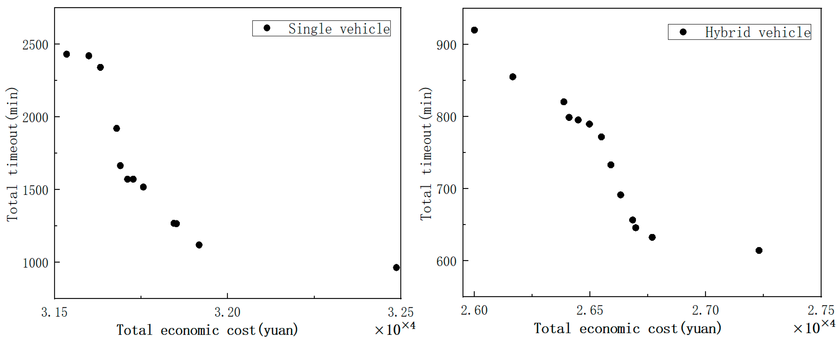
4.5. Comparative Analysis of Different Models

In this paper, comparisons are made under the same working conditions and other conditions. Figure 3 shows the comparison of Pareto fronts for single and hybrid models obtained by using the DCD-DE-NSGAII algorithm, and are shown in Table 10 shows the results of the two models.
Figure 3 shows that the Pareto optimal solution obtained by using a single (5 tons) vehicle model is significantly larger than the optimal solution obtained by using a hybrid (5 tons and 8 tons) vehicle model in terms of total timeout time and total economic cost. It can be concluded from Table 10 that the total economic cost, total overtime, carbon emissions cost, fuel consumption cost, vehicle use cost and wage cost of single vehicle are 16.61%, 55.34%, 18.68%, 18.68%, 16.14% and 16.91% higher than those of hybrid vehicle. It can be seen that government departments use hybrid models for clearing and transportation to save economic costs.
To further explore the differences between the two types of vehicles in terms of total driving distance, total fuel consumption, total service time, etc., this paper compares and analyzes the results obtained by decision makers when they prefer the optimal total economic cost, and obtains other results for different models as shown in Table 11; The comparative analysis of the single model and the hybrid model when the decision maker prefers the optimal total timeout time is similar to the previous one, which is not explained due to the space problem.
It is obvious from Table 11 that the total driving distance, total fuel consumption, total service time, total number of vehicles used and total number of departures of hybrid models are significantly lower than those of single models, which are 18.62%, 18.95%, 17.37%, 23.08% and 20.16% lower than those of single models respectively. Therefore, it can be seen that the use of mixed models by government departments can not only reduce the driving distance, save fuel consumption, reduce vehicle use, but also reduce the total service time and total number of departures, and effectively improve the efficiency of garbage removal.

5. Conclusions

This paper studies the scheduling problem of MSW removal vehicles with the factors of carbon emissions and time-dependent vehicle speed added. From the actual situation of MSW removal, the constraints of multiple models, multiple vehicle visits, different vehicle departure moments and time windows are considered, and a multi-objective model considering the economic cost and waste removal efficiency (the total overtime time response is the waste removal efficiency) is established, and an improved NSGA-II algorithm is proposed for the solution. The simulation results show that:
  • The model comprehensively considers environmental protection, economy and timeliness, and balances the interests between the government and garbage removal enterprises. The proposed optimization model is more in line with the actual situation of the current urban solid garbage removal and has strong practicability;
  • The dynamic congestion ranking strategy and differential variation operation are introduced into the NSGA-II algorithm, which improves the solution performance of the algorithm to some extent;
  • The model and algorithm proposed can effectively solve the vehicle scheduling problem of MSW removal considering the effect of time-dependent speed and carbon emissions. It can provide decision basis for decision makers with different preferences to choose reasonable waste removal paths and waste collection schemes.
  • In this paper, the results of the single model and the mixed model are compared and analyzed. The results show that the number of vehicles, the total driving distance, the total fuel consumption, the total service time and the cost of the mixed model are greatly reduced compared with the single model. It shows that the government departments can increase more heavy-duty garbage trucks, which can improve the efficiency of garbage removal, reduce the use of vehicles and reduce expenses;
  • In this paper, the different departure time of the vehicle is optimized reasonably, which can effectively avoid the traffic congestion period, shorten the driving time of the vehicle, improve the efficiency of garbage removal and reduce the economic cost.
The author established a multi-objective vehicle scheduling model for MSW removal from the static road network level which can be combined with GIS and other technologies to study the garbage collection and transportation problem of dynamic road network, making the research more realistic.

Author Contributions

Conceptualization, Z.G., Y.H. and X.X.; methodology, Y.H.; validation, Z.G., Y.H. and X.X.; formal analysis, Y.H.; investigation, X.X.; resources, Z.G., C.Z. and H.Z.; data curation, Y.H., H.W. and X.X.; writing—original draft preparation, Z.G., Y.H., X.X. and H.W.; writing—review and editing, Z.G., X.X., Y.H. and H.W.; visualization, Z.G.; supervision, Z.G. and C.Z. All authors have read and agreed to the published version of the manuscript.

Funding

This research was funded by the Science Research Project of Anhui Higher Education Institutes (No.2022AH040050), the Science Research Project of Anhui Higher Education Institutes (No.2022AH050269), the General Program of Anhui Natural Science Foundation [grant number 2208085MG181] and the Open Fund of Key Laboratory of Anhui Higher Education Institutes [grant number CS2021-ZD01].

Data Availability Statement

The data in this paper are from Ma’anshan City Administrative.

Conflicts of Interest

The authors declare no conflict of interest.

References

  1. Molina, J.C.; Eguia, I.; Racero, J. Reducing pollutant emissions in a waste collection vehicle routing problem using a variable neighborhood tabu search algorithm: A case study. TOP 2019, 27, 253–287. [Google Scholar] [CrossRef]
  2. Nurprihatin, F.; Lestari, A. Waste Collection Vehicle Routing Problem Model with Multiple Trips, Time Windows, Split Delivery, Heterogeneous Fleet and Intermediate Facility. Eng. J. 2020, 24, 55–64. [Google Scholar] [CrossRef]
  3. Farrokhi-Asl, H.; Tavakkoli-Moghaddam, R.; Asgarian, B. Metaheuristics for a bi-objective location-routing-problem in waste collection management. J. Ind. Prod. Eng. 2017, 34, 239–252. [Google Scholar] [CrossRef]
  4. Rabani, M.; Manavizadeh, N.; Boostani, A.; Aghamohamadi, S. A multi-objective model for the residential waste collection location-routing problem with time windows. J. Ind. Syst. Eng. 2020, 12, 227–241. [Google Scholar]
  5. Hina, S.M.; Szmerekovsky, J.; Lee, E.S.; Amin, M.; Arooj, S. Effective municipal solid waste collection using geospatial information systems for transportation: A case study of two metropolitan cities in Pakistan. Res. Transp. Econ. 2020, 84, 100950. [Google Scholar] [CrossRef]
  6. Ahlaqqach, M.; Benhra, J.; Mouatassim, S.; Lamrani, S. Multi-objective Optimization of Heterogeneous Vehicles Routing in the Case of Medical Waste Using Genetic Algorithm. Smart Appl. Data Anal. 2020, 1207, 256–269. [Google Scholar]
  7. Dereci, U.; Karabekmez, M.E. The applications of multiple route optimization heuristics and meta-heuristic algorithms to solid waste transportation: A case study in Turkey. Decis. Anal. J. 2022, 4, 100113. [Google Scholar] [CrossRef]
  8. Niu, Y.Y.; Yang, Z.H.; Chen, P.; Xiao, J. Optimizing the green open vehicle routing problem with time windows by minimizing comprehensive routing cost. J. Clean. Prod. 2018, 171, 962–971. [Google Scholar] [CrossRef]
  9. Rauniyar, A.; Nath, R.; Muhuri, P.K. Multi-factorial evolutionary algorithm based novel solution approach for multi-objective pollution-routing problem. Comput. Ind. Eng. 2019, 130, 757–771. [Google Scholar] [CrossRef]
  10. Qiu, J.; Sun, J.; Zhong, Z. A multi-objective green vehicle routing optimization algorithm based on delivery benefit blance. Control Decis. 2023, 38, 365–371. [Google Scholar] [CrossRef]
  11. Zhou, G.; Ji, B.; Fang, X. Research on green vehicle routing problem and algorithm of multi-to-many cross-docking. J. Railw. Sci. Eng. 2022, 19, 2202–2210. [Google Scholar] [CrossRef]
  12. Zhou, X.; Jiang, T.; He, C.; Wang, L.; Yang, L. Green Vehicle Routing Model and Its Solution Algorithm in Cold-chain Logistics Distribution. Chin. J. Manag. Sci. 2016, 1–11. [Google Scholar] [CrossRef]
  13. Erdoğdu, K.; Karabulut, K. Bi-objective green vehicle routing problem. Int. Trans. Oper. Res. 2022, 29, 1602–1626. [Google Scholar] [CrossRef]
  14. Soysal, M.; Çimen, M.; Mine, Ö.; Belbağ, S. Performance Comparison of Two Recent Heuristics for Green Time Dependent Vehicle Routing Problem. Int. J. Bus. Anal. 2019, 6, 11. [Google Scholar] [CrossRef]
  15. Çimen, M.; Soysal, M. Time-dependent green vehicle routing problem with stochastic vehicle speeds: An approximate dynamic programming algorithm. Transp. Res. Part D Transp. Environ. 2017, 54, 82–98. [Google Scholar] [CrossRef]
  16. Zhou, X.; Liu, C.; Zhou, K.J.; He, C.H.; Huang, X. Improved ant colony algorithm and modeling of time-dependent green vehicle routing problem. J. Manag. Sci. China 2019, 22, 57–68. [Google Scholar]
  17. Zhou, X.; Lv, Y.; He, C.; Liu, C.; Yang, K. Multi-depot green vehicle routing model and its optimization algorithm with time-dependent speed. Control Decis. 2022, 37, 473–482. [Google Scholar] [CrossRef]
  18. Ge, X.; Ran, X. Study on the Optimization of Pollution Routing Problem with Time-dependent Traffic Congestion. Ind. Eng. Manag. 2020, 25, 75–93. [Google Scholar]
  19. Chen, C.; Liu, Y.P.; Lin, Q.T.; Li, Q.N. On Time and Space Dependent Vehicle Routing Problem in Urban Delivery. Ind. Eng. Manag. 2021, 26, 56–62. [Google Scholar]
  20. Zhu, L.; Ma, X.; Liu, Z. Time-dependent Green Vehicle Routing Problem. J. Transp. Syst. Eng. Inf. Technol. 2021, 21, 187–194. [Google Scholar] [CrossRef]
  21. Luo, H.; Dridi, M.; Grunder, O. A branch-price-and-cut algorithm for a time-dependent green vehicle routing problem with the consideration of traffic congestion. Comput. Ind. Eng. 2023, 177, 109093. [Google Scholar] [CrossRef]
  22. Liu, Y.; Roberto, B.; Zhou, J.; Yu, Y.; Zhang, Y.; Sun, W. Efficient Feasibility Checks and an Adaptive Large Neighborhood Search Algorithm for the Time-Dependent Green Vehicle Routing Problem with Time Windows. Eur. J. Oper. Res. 2023, in press. [Google Scholar] [CrossRef]
  23. Deb, K.; Agrawal, S.; Pratap, A.; Meyarivan, T. A Fast Elitist Non-dominated Sorting Genetic Algorithm for Multi-objective Optimization: NSGA-II. In Proceedings of the 6th International Conference, Paris, France, 18–20 September 2000; pp. 849–858. [Google Scholar] [CrossRef]
  24. Deb, K.; Pratap, A.; Agarwal, S.; Meyarivan, T. A fast and elitist multiobjective genetic algorithm: NSGA-II. IEEE Trans. Evol. Comput. 2002, 6, 182–197. [Google Scholar] [CrossRef] [Green Version]
  25. Verma, S.; Pant, M.; Snasel, V. A comprehensive review on NSGA-II for multi-objective combinatorial optimization problems. IEEE Access 2021, 9, 57757–57791. [Google Scholar] [CrossRef]
  26. Xu, H.; Fan, W.; Wei, T.; Yu, L. An Or-opt NSGA-II algorithm for multi-objective Vehicle Routing Problem with Time Windows. In Proceedings of the 2008 IEEE International Conference on Automation Science and Engineering, Arlington, VA, USA, 23–26 August 2008; pp. 309–314. [Google Scholar] [CrossRef]
  27. Liu, Y.Y.; Enayatollahi, F.; Thulasiraman, P. Traffic aware many-objective dynamic route planning. In Proceedings of the 2019 IEEE Symposium Series on Computational Intelligence (SSCI), Xiamen, China, 6–9 December 2019; pp. 1241–1248. [Google Scholar]
  28. Wang, Y.; Zhang, J.; Assogba, K.; Liu, Y.; Xu, M.; Wang, Y. Collaboration and transportation resource sharing in multiple centers vehicle routing optimization with delivery and pickup. Knowl. Based Syst. 2018, 160, 296–310. [Google Scholar] [CrossRef]
  29. Srivastava, G.; Singh, A.; Mallipeddi, R. NSGA-II with objective-specific variation operators for multiobjective vehicle routing problem with time windows. Expert Syst. Appl. 2021, 176, 114779. [Google Scholar] [CrossRef]
  30. Barth, M.; Younglove, T.; Scora, G. Development of a Heavy-Duty Diesel Modal Emissions and Fuel Consumption Model; UC Berkeley; California Partners for Advanced Transportation Technology: Berkeley, CA, USA, 2005. [Google Scholar]
  31. Shi, S.; Zhang, X.; Wang, Z. An Improved NSGA-Il Algorithm Based on Dynamic Crowding Distance and Adaptive t-Distribution Crossover. Comput. Simul. 2019, 36, 257–262. [Google Scholar]
  32. Zheng, X.; Ma, L. An improved NSGA-II algorithm for multi-objective nonlinear optimization. Microelectron. Comput. 2020, 37, 47–53. [Google Scholar]
Figure 1. DCD-DE-NSGAII algorithm flowchart.
Systems 11 00173 g001
Figure 2. Comparison chart of two algorithms pareto frontier.
Systems 11 00173 g002
Figure 3. Pareto frontier comparison of two models.
Systems 11 00173 g003
Table 1. The meanings of variables, sets, and decision variables.
SymbolMeaningSymbolMeaning
P Collection of refuse transfer stations, P = 1 , 2 , 3 . N ; C Municipal sanitation department and waste incineration plant collection, C = 0 , N + 1 ;
A Node set, A = P     C ; E Road set between nodes;
D i j The distance from node i to node j ; H Vehicle h set, H = 1 , 2 , 3 , . n q + n z ;
n q Number of light-duty garbage trucks; n z Number of heavy-duty garbage trucks;
H Q q The maximum load of light load garbage trucks; H Q z The maximum load of heavy-duty garbage truck;
H Q Maximum load collection of garbage trucks; H Q = H Q q     H Q z ; Q i Daily garbage volume of transfer station i ;
q i h The amount of garbage loaded by vehicle h at transfer station i ; L T i The latest time that each transfer station allows service;
K The set of time period k ; b k The start time of time period k ;
e k The end time of time period k ; v f Vehicle speed in non-congested time period;
v c Vehicle speed during congested time periods; β i h Time of arrival of vehicle h to transfer station;
l i h Time of vehicle h leaving transfer station i ; s i h Service time of vehicle h at transfer station i ;
A T i The time when all the garbage in the transfer station has been removed; C f Unit fuel consumption cost, unit one liter;
C e Unit carbon emissions cost, unit kg; μ Unit time cost of vehicle use, unit min;
ψ Driver unit time wage cost, unit hour; ζ Fixed departure fee for garbage truck, unit vehicle; ζ = ζ q ζ z ;
ζ q Light-duty garbage truck fixed departure fee, unit vehicle; ζ z Heavy-duty garbage truck fixed departure cost, unit vehicle;
V i j k The speed of the vehicle on the road i , j during time period k ; t i j k The time of vehicle h running the whole road i , j ;
d i j k h The mileage of vehicle h on road i , j at speed V i j k in time period k ; t i j k h The time that vehicle h travels on the road i , j at speed V i j k in time period k ;
F C i j k h The fuel consumption of vehicle h on road i , j in time period k , unit one liter; E C i j k h The carbon emissions of vehicle h on road i , j in time period k , unit kg;
X i h 0–1 variable with a value of 1 when transit station i is served by vehicle h and 0 otherwise; X i j 0–1 variable, which is 1 when there is a vehicle on the road, otherwise 0;
σ h 0–1 variable, 1 when the vehicle is used, 0 otherwise; y i j h 0–1 variable, when the vehicle h travels from node i to node j , it is 1, otherwise it is 0.
Z i j k h 0–1 variable, 1 when vehicle h travels from node i to node j in time period k , 0 otherwise;
Table 2. Garbage transfer station information.
Serial NumberSite NameX-Coordinate (m)Y-Coordinate (m)Average Daily Refuse Production (t)Time Window
1City Administration33,250,196.37,531,852.0——[5:30–18:00]
2Wangjiashan33,246,232.17,535,882.442.00738
3Oriental Pearl33,249,124.57,527,993.124.00958
4Xiangyang33,256,135.77,532,931.625.78518
5Oriental City33,250,892.17,531,310.027.60692
6Sixth Middle School33,246,145.47,530,181.736.69531
7Junmin Road33,249,685.57,532,563.738.74942
8Nantang33,247,479.07,527,277.210.52482
9Zhongcun33,245,589.97,527,948.315.00852
10Yongtai33,244,264.57,530,779.912.00872
11Rainfield33,244,685.27,534,773.123.08897
12Harvest Garden33,252,294.87,528,515.531.42521
13Sand pond33,246,762.07,529,212.020.00672
14Zhaoming33,247,914.77,524,648.22.66605
15Jinshan Road33,247,578.57,537,081.816.58864
16Quarrying stone33,242,389.47,533,118.611.00687
17Jin’an Jiayuan33,247,757.87,528,040.527.28917
18Jin Rui33,249,534.57,527,329.223.36567
19West Lake Garden33,249,676.47,529,831.855.46607
20New workshop33,245,222.57,527,303.04.82550
21Hengxing33,244,276.67,527,534.34.50545
22Ten districts33,244,746.27,530,784.727.12897
23Yingcui33,244,726.57,532,763.138.80758
24Pearl garden33,246,910.17,531,456.936.08744
25Plum garden33,248,855.27,531,184.538.99550
26Spring light33,249,306.67,532,285.639.00889
27Royal view garden33,253,746.87,532,021.46.66779
28Xiangshan Waste Incineration Plant33,262,273.87,532,404.0————
Table 3. Distribution vehicle information.
Vehicle TypeVehicle CountWeight/(t)Load/(t)Cost/(Yuan)
light load3785200
heavy load8108300
Table 4. Model parameter information.
SignParameter ValueSignParameter ValueSignParameter Value
C f 6.5 yuan/L C e 0.0528 yuan/kg. μ 1.5 yuan/min
ψ 0.5 yuan/min ζ q 200 yuan/car ζ z 300 yuan/car
α 1 1 . 4   ×   10 - 6 α 2 4 . 35   ×   10 - 10 α 3 1 . 04   ×   10 - 11
F E 2.621 kg/L V f 600 m/min V c 300 m/min
Table 5. Statistical results of different algorithms.
AlgorithmTotal Economic Cost/(Yuan)Total Timeout/(min)
Optimal SolutionWorst SolutionAverage SolutionOptimal SolutionWorst SolutionAverage Solution
NSGAII26,618.0027,183.0026,869.43633.181355.80931.94
DCD-DE-NSGAII25,940.0027,217.0026,503.38615.16921.15748.51
Improved ratio2.55−0.121.362.8532.119.68
Table 7. Vehicle routing scheduling scheme.
Vehicle NumberVehicle TypeVehicle Scheduling PathDeparture Times
1heavy load1–19–28–19–28–27–12–28–22–23–28–17–28–26–28–11–28–17
2heavy load1–19–28–19–28–4–28–6–22–28–5–28–18–28–11–28–17
3heavy load1–19–28–14–21–12–6–28–10–16–28–18–25–28–11–28–15
4light load1–19–28–27–28–4–28–23–28–17–28–25–26–28–7–28–17
5heavy load1–19–28–12–28–22–28–24–17–28–26–28–7–28–16
6light load1–19–14–28–6–28–24–28–2–28–7–28–15
7heavy load1–13–28–4–6–28–24–28–2–28–7–28–15
8light load1–13–28–6–28–24–28–2–28–7–28–15
9heavy load1–13–12–28–22–28–5–28–25–28–7–28–15
10light load1–12–28–6–28–24–28–18–28–15–28–15
11heavy load1–12–28–23–28–5–28–25–28–15–28–15
12light load1–4–28–23–28–5–17–2–28–15–28–14
13light load1–6–28–23–16–28–2–28–3–28–14
14light load1–6–28–20–24–28–18–28–3–28–14
15heavy load1–6–28–16–28–2–25–28–3–28–14
16light load1–22–28–24–28–25–28–3–28–14
17light load1–23–28–17–28–25–28–3–28–14
18light load1–23–28–2–28–12
19light load1–10–28–2–28–12
20light load1–16–17–28–25–28–12
21light load1–24–28–25–28–12
22light load1–26–28–11
23light load1–26–28–11
24light load1–26–28–11
25light load1–26–8–9–28–11
26light load1–8–28–11
27light load1–8–28–11
28light load1–9–28–11
29light load1–9–28–11
30light load1–9–28–11
Total 103
Table 8. Optimization table of vehicle clearance time.
Vehicle NumberVehicle TypeVehicle Clearance Time
1heavy load330–333.48–374.91–396.33–445.53–473.98–496.63–551.16–580.50–593.80–643.05–668.31–713.57–735.19–776.80–899.58–949.16–969.31
2heavy load348–351.48–392.91–414.33–477.19–497.73–538.26–566.27–578.81–628.14–647.20–686.26–709.11–751.97–899.58–949.16–969.31
3heavy load362–365.48–406.91–448.21–473.69–510.62–540.93–588.06–618.20–633.19–686.36–709.21–725.74–768.19–899.58–949.16–969.31
4light load381–384.48–425.91–454.36–502.81–523.34–556.94–586.19–635.44–660.71–705.97–728.43–740.41–782.02–890.98–931.96–952.11
5heavy load397–400.48–453.81–489.51–545.21–574.55–623.88–649.54–665.41–710.67–732.28–773.89–890.98–931.96–952.11
6light load412–415.48–443.73–518.13–556.19–603.33–628.99–674.64–702.00–749.36–890.98–931.96–952.11
7heavy load425–439.44–512.23–532.76–560.03–607.17–632.82–678.48–705.84–753.19–890.98–931.96–952.11
8light load436–450.44–523.23–558.75–605.88–631.54–677.19–704.55–751.91–890.98–931.96–952.11
9heavy load453–467.44–496.03–550.86–580.20–629.54–648.59–687.65–710.11–752.56–890.98–931.96–952.11
10light load468–481.14–536.84–565.55–612.69–638.34–684.00–706.85–749.71–895.70–941.41–961.56
11heavy load485–498.14–551.92–581.17–630.42–649.48–688.54–711–753.45–895.71–941.41–961.56
12light load500–520.12–555.33–584.58–633.83–652.89–670.44–693.75–741.11–895.70–941.41–961.56
13light load519–533.61–580.74–610.00–623.94–677.09–704.45–751.81–893.12–936.23–956.38
14light load533–543.80–590.94–620.60–638.07–683.73–706.58–749.43–893.12–936.23–956.38
15heavy load541–548.30–595.44–628.60–681.76–709.12–728.09–770.54–893.12–936.23–956.38
16light load561–570.26–619.59–645.25–690.90–713.36–755.82–893.12–936.23–956.38
17light load576–585.24–634.49–659.76–705.02–727.48–769.93–893.12–936.23–956.38
18light load592–601.24–650.49–677.85–725.21–890.15
19light load602–612.05–662.18–689.54–736.90–890.15
20light load623–636.18–658.49–703.76–726.22–768.67–890.15
21light load639–644.52–690.17–712.63–755.08–890.15
22light load848–849.65–891.26–911.41
23light load849–850.65–892.26–912.41
24light load860–861.65–903.26–923.41
25light load861–862.64–881.54–894.88–943.66–963.81
26light load865–873.87–919.96–940.11
27light load870–878.87–924.96–945.11
28light load875–885.06–933.84–953.99
29light load878–888.06–936.84–956.99
30light load888–898.06–946.84–966.99
Table 9. Comparison of results of different preferences.
f 1 * Total Driving Distance/(km)Total Fuel Consumption/(L)Total Service Time/(min)Number of Vehicles Used/(Vehicle)Total Number of Departures/(Times)
f 1 3111.08458.677962.5630103
f 2 3266.19479.418268.9431108
Table 10. Comparison of the results of the two models.
Vehicle TypeTotal Economic Cost/(Yuan)Total Timeout /(min)Fuel Consumption Cost/(Yuan)Carbon Emissions Cost/(Yuan)Vehicle Cost /(Yuan)Wage Cost /(Yuan)
Single model31,784.041675.843693.41786.3522,474.044830.24
Hybrid model26,503.38748.513003.42639.4518,847.314013.21
Optimized ratio%16.6155.3418.6818.6816.1416.91
Table 11. Comparison of other results of different models.
Vehicle TypeTotal Driving Distance/(km)Total Fuel Consumption/(L)Total Service Time/(min)Number of Vehicles Used/(Vehicle)Total Number of Departures/(Time)
Single model3822.9565.949636.0139129
Hybrid model31,11.08458.677962.5630103
Optimized ratio%18.6218.9517.3723.0820.16
Disclaimer/Publisher’s Note: The statements, opinions and data contained in all publications are solely those of the individual author(s) and contributor(s) and not of MDPI and/or the editor(s). MDPI and/or the editor(s) disclaim responsibility for any injury to people or property resulting from any ideas, methods, instructions or products referred to in the content.

