

An Integrated EDAS Model for Fermatean Fuzzy Multi-Attribute Group Decision Making and Its Application in Green-Supplier Selection

Abstract
:1. Introduction
- (1)
- Uncertainty exists in the evaluation standards of green suppliers. The information conveyed by IFSs and PFSs was limited. Few GSS studies considered the usefulness of Fermatean fuzzy (FF) evaluation information.
- (2)
- (3)
- (4)
- BWM [20] and AHP [21] were subjective weighting methods dominated by experts’ subjective judgments. It is impossible to make a fully reasonable judgment on the importance of indicators without the joint participation of objective weighting methods. Furthermore, it is crucial to apply precise and consistent evaluation methods when ranking alternative solutions. Decision methods such as VIKOR [14] and TOPSIS [22] may increase the negative impact of extreme value decision results.
- (1)
- The GSS problem in the FF environment will be examined, where FFSs have a broader range of information representation.
- (2)
- Create a comprehensive set of index systems for evaluating green suppliers. This study developed a set of index systems combining traditional qualities, green attributes, and social attributes based on references and analysis of the existing index system.
- (3)
- We propose the FFPHM and FFWPHM operators by applying the PHM operator to the FF environment. The proposed operators consider the consistency and correlation of data when aggregating evaluation information.
- (4)
- For the GSS problem that it is unknown how important the various indicators are, an integrated weight calculation method is offered in the foundations of EWM and BWM. This integrated technique successfully lowers the disparity between subjective and objective information.
- (5)
- A FF MAGDM framework based on the integrated weight determination model and EDAS is developed. EDAS simplifies the calculation process while reducing the impact of extreme values on decision results. The method improves and deepens fuzzy decision theory and gives specialists technical direction for resolving GSS issues.
2. Literature Review
2.1. FFSs
2.2. Power Heronian Mean Aggregation Operators
2.3. BWM and EWM for Attribute Weights
2.4. Evaluation Methods for GSS
3. Evaluation Index System for GSS
4. Fermatean Fuzzy Power Heronian Mean Aggregation Operators
5. Fermatean Fuzzy MAGDM Model Based on the Integrated EDAS Method
5.1. Integrated Weight Based on BWM and Fermatean Fuzzy Entropy
- (1)
- Objective weight determination based on the EWM.
- (2)
- Subjective weight determination method based on the BWM.
- (3)
- Integrated weight determination method based on the BWM and EWM.
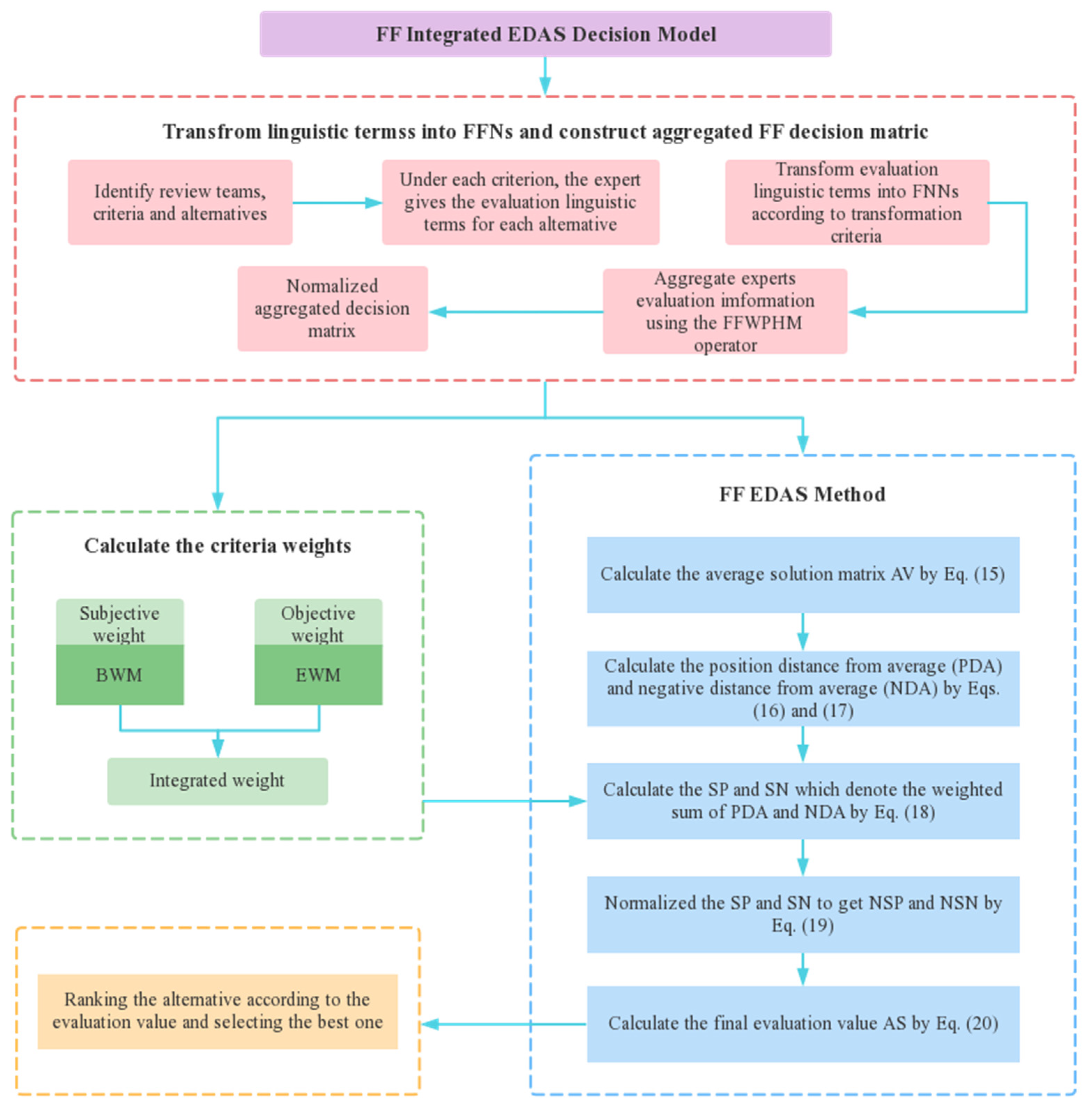
5.2. Procedure of Fermatean Fuzzy Integrated EDAS Model
6. Case Study
6.1. Sensitivity Analysis
6.2. Comparative Analysis
- (1)
- In regard to the ranking approach, it is not suitable to utilize the closeness degree formula that was finally employed for ranking in [17] when an alternative to being considered is a positive ideal solution. The concept of superior and inferior solutions is transformed by EDAS into a compromise idea, which significantly improves the influence of extreme values on the decision outcome. The FF weighted average (FFWA) operator engaged in research [26,27] may result in information loss and even rank inability when membership or non-membership is equal to zero in the FF environment.
- (2)
- Only simple decision-making environments are covered by [17,27]. Due to insufficient information and poor consideration, a single DM might not be capable of making appropriate decisions. Meanwhile, the introduction of the FFWA operator into the MAGDM by [26] may cause incorrect initial assessment information aggregation. The decision-making model proposed assumes the participation of numerous DMs, and the choice results generated by the group of DMs with their collective wisdom are more practical to implement.
- (3)
- All other approaches engaged in the comparison only focus on the objective data and consider the objective weights of attributes in their investigations but neglect the subjective judgment of DMs, which is a main drawback. Subjective weights are rather realistic and aid in lowering the bias of the results. The integrated weighting technique constructed can measure the importance of attributes more comprehensively and also addresses the unscientific effects brought on by too strong subjective psychology in the calculation.
7. Conclusions
Author Contributions
Funding
Data Availability Statement
Conflicts of Interest
Appendix A
- (1)
- ;
- (2)
- ;
- (3)
- ;
- (4)
- ;
- (5)
- .
- (1)
- if , then ;
- (2)
- if , then,
- (a)
- if , then ;
- (b)
- if , then .
- (1)
- ;
- (2)
- ;
- (3)
- If , then .
References
- Wang, D.W.; Li, J. Coastal haze pollution, economic and financial performance, and sustainable transformation in coastal cities. J. Coast. Res. 2020, 109, 1–7. [Google Scholar] [CrossRef]
- Ahmed, Z.; Asghar, M.M.; Malik, M.N.; Nawaz, K. Moving towards a sustainable environment: The dynamic linkage between natural resources, human capital, urbanization, economic growth, and ecological footprint in China. Resour. Policy 2020, 67, 101677. [Google Scholar] [CrossRef]
- Zhang, K.M.; Wen, Z.G. Review and challenges of policies of environmental protection and sustainable development in China. J. Environ. Manag. 2008, 88, 1249–1261. [Google Scholar] [CrossRef] [PubMed]
- Tseng, C.H.; Chang, K.H.; Chen, H.W. Strategic orientation, environmental innovation capability, and environmental sustainability performance: The case of Taiwanese suppliers. Sustainability 2019, 11, 1127. [Google Scholar] [CrossRef] [Green Version]
- Cabral, I.; Grilo, A.; Cruz-Machado, V. A decision-making model for lean, agile, resilient and green supply chain management. Int. J. Prod. Res. 2012, 50, 4830–4845. [Google Scholar] [CrossRef]
- Hervani, A.A.; Helms, M.M.; Sarkis, J. Performance measurement for green supply chain management. Benchmarking Int. J. 2005, 12, 330–353. [Google Scholar] [CrossRef] [Green Version]
- Gupta, H.; Barua, M.K. Supplier selection among SMEs on the basis of their green innovation ability using BWM and fuzzy TOPSIS. J. Clean. Prod. 2017, 152, 242–258. [Google Scholar] [CrossRef]
- Rajesh, R.; Ravi, V. Supplier selection in resilient supply chains: A grey relational analysis approach. J. Clean. Prod. 2015, 86, 343–359. [Google Scholar] [CrossRef]
- Zhu, W.; He, Y. Green product design in supply chains under competition. Eur. J. Oper. Res. 2017, 258, 165–180. [Google Scholar] [CrossRef]
- Boran, F.E.; Genç, S.; Kurt, M.; Akay, D. A multi-criteria intuitionistic fuzzy group decision making for supplier selection with TOPSIS method. Expert Syst. Appl. 2009, 36, 11363–11368. [Google Scholar] [CrossRef]
- Govindan, K.; Rajendran, S.; Sarkis, J.; Murugesan, P. Multi criteria decision making approaches for green supplier evaluation and selection: A literature review. J. Clean. Prod. 2015, 98, 66–83. [Google Scholar] [CrossRef]
- Banaeian, N.; Mobli, H.; Fahimnia, B.; Nielsen, I.E.; Omid, M. Green supplier selection using fuzzy group decision making methods: A case study from the agri-food industry. Comput. Oper. Res. 2018, 89, 337–347. [Google Scholar] [CrossRef]
- Kilic, H.S.; Yalcin, A.S. Modified two-phase fuzzy goal programming integrated with IF-TOPSIS for green supplier selection. Appl. Soft Comput. 2020, 93, 106371. [Google Scholar] [CrossRef]
- Zhou, F.; Chen, T.Y. An integrated multicriteria group decision-making approach for green supplier selection under Pythagorean fuzzy scenarios. IEEE Access 2020, 8, 165216–165231. [Google Scholar] [CrossRef]
- Atanassov, K.T. Intuitionistic fuzzy sets. Fuzzy Sets Syst. 1986, 20, 1–137. [Google Scholar] [CrossRef]
- Yager, R.R. Pythagorean membership grades in multicriteria decision making. IEEE Trans. Fuzzy Syst. 2013, 22, 958–965. [Google Scholar] [CrossRef]
- Senapati, T.; Yager, R.R. Fermatean fuzzy sets. J. Ambient Intell. Hum. Comput. 2020, 11, 663–674. [Google Scholar] [CrossRef]
- Nguyen, N.B.T.; Lin, G.H.; Dang, T.T. A Two phase integrated fuzzy decision-making framework for green supplier selection in the coffee bean supply chain. Mathematics 2021, 9, 1923. [Google Scholar] [CrossRef]
- Tavana, M.; Shaabani, A.; Santos-Arteaga, F.J.; Valaei, N. An integrated fuzzy sustainable supplier evaluation and selection framework for green supply chains in reverse logistics. Environ. Sci. Pollut. Res. 2021, 28, 53953–53982. [Google Scholar] [CrossRef]
- Fazlollahtabar, H.; Kazemitash, N. Green supplier selection based on the information system performance evaluation using the integrated Best-Worst Method. Facta Univ. Ser. Mech. Eng. 2021, 19, 345–360. [Google Scholar] [CrossRef]
- Wang, C.N.; Nguyen, T.L.; Dang, T.T. Two-Stage Fuzzy MCDM for Green Supplier Selection in Steel Industry. Intell. Autom. Soft Comput. 2022, 33, 1245–1260. [Google Scholar] [CrossRef]
- Çalık, A. A novel Pythagorean fuzzy AHP and fuzzy TOPSIS methodology for green supplier selection in the Industry 4.0 era. Soft Comput. 2021, 25, 2253–2265. [Google Scholar] [CrossRef]
- Zeng, S.Z.; Pan, Y.; Jin, H.H. Online Teaching Quality Evaluation of Business Statistics Course Utilizing Fermatean Fuzzy Analytical Hierarchy Process with Aggregation Operator. Systems 2022, 10, 63. [Google Scholar] [CrossRef]
- Wei, D.M.; Meng, D.; Rong, Y.; Liu, Y.; Garg, H.; Pamucar, D. Fermatean Fuzzy Schweizer–Sklar Operators and BWM-Entropy-Based Combined Compromise Solution Approach: An Application to Green Supplier Selection. Entropy 2022, 24, 776. [Google Scholar] [CrossRef] [PubMed]
- Tan, J.D.; Liu, Y.; Senapati, T.; Grag, H.; Rong, Y. An extended MABAC method based on prospect theory with unknown weight information under Fermatean fuzzy environment for risk investment assessment in B&R. J. Ambient Intell. Hum. Comput. 2022, 1–30. [Google Scholar] [CrossRef]
- Mishra, A.R.; Rani, P. Multi-criteria healthcare waste disposal location selection based on Fermatean fuzzy WASPAS method. Complex Intell. Syst. 2021, 7, 2469–2484. [Google Scholar] [CrossRef]
- Gül, S. Fermatean fuzzy set extensions of SAW, ARAS, and VIKOR with applications in COVID-19 testing laboratory selection problem. Expert Syst. 2021, 38, e12769. [Google Scholar] [CrossRef]
- Yager, R.R. The power average operator. IEEE Trans. Syst. Man Cybern. Part A Syst. Hum. 2001, 31, 724–731. [Google Scholar] [CrossRef]
- Beliakov, G.; Pradera, A.; Calvo, T. Aggregation Functions: A Guide for Practitioners; Springer: Berlin/Heidelberg, Germany, 2007; Volume 221. [Google Scholar]
- Shi, M.H.; Yang, F.; Xiao, Y. Intuitionistic fuzzy power geometric Heronian mean operators and their application to multiple attribute decision making. J. Intell. Fuzzy Syst. 2019, 37, 2651–2669. [Google Scholar] [CrossRef]
- Liu, P.D.; Mahmood, T.; Khan, Q. Group decision making based on power Heronian aggregation operators under linguistic neutrosophic environment. Int. J. Fuzzy Syst. 2018, 20, 970–985. [Google Scholar] [CrossRef]
- Rezaei, J. Best-worst multi-criteria decision-making method. Omega 2015, 53, 49–57. [Google Scholar] [CrossRef]
- Liu, S.; Zhang, J.X.; Niu, B.; Liu, L.; He, X.J. A novel hybrid multi-criteria group decision-making approach with intuitionistic fuzzy sets to design reverse supply chains for COVID-19 medical waste recycling channels. Comput. Ind. Eng. 2022, 169, 108228. [Google Scholar] [CrossRef] [PubMed]
- Ma, Y.F.; Zhao, Y.Y.; Wang, X.Y.; Feng, C.Y.; Zhou, X.Y.; Lev, B. Integrated BWM-Entropy weighting and MULTIMOORA method with probabilistic linguistic information for the evaluation of Waste Recycling Apps. Appl. Intell. 2023, 53, 813–816. [Google Scholar] [CrossRef]
- Feng, D.; Fu, X.Y.; Jiang, S.F.; Jing, L.T. Conceptual Solution Decision Based on Rough Sets and Shapley Value for Product-Service System: Customer Value-Economic Objective Trade-Off Perspective. Appl. Sci. 2021, 11, 11001. [Google Scholar] [CrossRef]
- Krishankumar, R.; Arun, K.; Kumar, A.; Rani, P.; Ravichandran, K.S.; Gandomi, A.H. Double-hierarchy hesitant fuzzy linguistic information-based framework for green supplier selection with partial weight information. Neural Comput. Appl. 2021, 33, 14837–14859. [Google Scholar] [CrossRef]
- Xiong, L.; Zhong, S.Q.; Liu, S.; Zhang, X.; Li, Y.F. An approach for resilient-green supplier selection based on WASPAS, BWM, and TOPSIS under intuitionistic fuzzy sets. Math. Probl. Eng. 2020, 2020. [Google Scholar] [CrossRef]
- Liu, P.; Pan, Q.; Xu, H.X.; Zhu, B.Y. An Extended QUALIFLEX Method with Comprehensive Weight for Green Supplier Selection in Normal q-Rung Orthopair Fuzzy Environment. Int. J. Fuzzy Syst. 2022, 24, 2174–2202. [Google Scholar] [CrossRef]
- Baki, R. An Integrated Multi-criteria Structural Equation Model for Green Supplier Selection. Int. J. Precis. Eng. Manuf. Green Technol. 2022, 9, 1063–1076. [Google Scholar] [CrossRef]
- Zhang, S.Q.; Wei, G.W.; Gao, H.; Wei, C.; Wei, Y. EDAS method for multiple criteria group decision making with picture fuzzy information and its application to green suppliers selections. Technol. Econ. Dev. Econ. 2019, 25, 1123–1138. [Google Scholar] [CrossRef] [Green Version]
- Zhang, N.; Su, W.H.; Zhang, C.H.; Zeng, S.Z. Evaluation and selection model of community group purchase platform based on WEPLPA-CPT-EDAS method. Comput. Ind. Eng. 2022, 172, 108573. [Google Scholar] [CrossRef]
- Mishra, A.R.; Rani, P.; Pandey, K. Fermatean fuzzy CRITIC-EDAS approach for the selection of sustainable third-party reverse logistics providers using improved generalized score function. J. Ambient Intell. Hum. Comput. 2022, 13, 295–311. [Google Scholar] [CrossRef] [PubMed]
- He, Y.; Wei, G.W.; Chen, X.D. Taxonomy-based multiple attribute group decision making method with probabilistic uncertain linguistic information and its application in supplier selection. J. Intell. Fuzzy Syst. 2021, 41, 3237–3250. [Google Scholar] [CrossRef]
- Xu, D.S.; Cui, X.X.; Xian, H.X. An extended EDAS method with a single-valued complex neutrosophic set and its application in green supplier selection. Mathematics 2020, 8, 282. [Google Scholar] [CrossRef] [Green Version]
- Wu, Y.N.; Xu, C.B.; Huang, Y.; Li, X.Y. Green supplier selection of electric vehicle charging based on Choquet integral and type-2 fuzzy uncertainty. Soft Comput. 2020, 24, 3781–3795. [Google Scholar] [CrossRef]
- Kang, X.; Xu, X.J.; Yang, Z.L. Evaluation and selection of green suppliers for papermaking enterprises using the interval basic probability assignment-based intuitionistic fuzzy set. Complex Intell. Syst. 2022, 8, 4187–4203. [Google Scholar] [CrossRef]
- Gegovska, T.; Koker, R.; Caka, T. Green supplier selection using fuzzy multiple-criteria decision-making methods and artificial neural networks. Comput. Intell. Neurosci. 2020, 2020. [Google Scholar] [CrossRef]
- Krishankumar, R.; Gowtham, Y.; Ahmed, I.; Ravichandran, K.S.; Kar, S. Solving green supplier selection problem using q-rung orthopair fuzzy-based decision framework with unknown weight information. Appl. Soft Comput. 2020, 94, 106431. [Google Scholar] [CrossRef]
- Deng, Z.; Wang, J.Y. Evidential Fermatean fuzzy multicriteria decision-making based on Fermatean fuzzy entropy. Int. J. Intell. Syst. 2021, 36, 5866–5886. [Google Scholar] [CrossRef]
- Liu, P.D.; Chen, S.M.; Wang, P. Multiple-attribute group decision-making based on q-rung orthopair fuzzy power maclaurin symmetric mean operators. IEEE Trans. Syst. Man Cybern. Syst. 2018, 50, 3741–3756. [Google Scholar] [CrossRef]


| Evaluation Criteria | [18] | [19] | [20] | [21] | [22] | [36] | [37] | [38] | [39] | [44] | [45] | [46] | [47] | [48] | Occurrence Percentage |
|---|---|---|---|---|---|---|---|---|---|---|---|---|---|---|---|
| Green design | √ | √ | √ | √ | √ | √ | √ | √ | √ | 64.29% | |||||
| Service | √ | √ | √ | √ | √ | √ | √ | 50.00% | |||||||
| Green image | √ | √ | √ | √ | √ | √ | 42.86% | ||||||||
| Quality | √ | √ | √ | √ | √ | √ | √ | √ | √ | √ | √ | 78.57% | |||
| Environmental management | √ | √ | √ | √ | √ | √ | √ | √ | √ | 64.29% | |||||
| Green product | √ | √ | √ | √ | 28.57% | ||||||||||
| Delivery | √ | √ | √ | √ | √ | √ | √ | √ | √ | √ | 71.43% | ||||
| Cost | √ | √ | √ | √ | √ | √ | √ | √ | √ | √ | √ | 78.57% | |||
| Technology | √ | √ | √ | √ | √ | √ | 42.86% | ||||||||
| Pollution control | √ | √ | √ | √ | √ | √ | √ | 50.00% | |||||||
| Energy resource utilization | √ | √ | √ | √ | √ | 35.71% | |||||||||
| Social responsibility | √ | √ | 14.29% | ||||||||||||
| Cooperation | √ | √ | √ | √ | 28.57% |
| Linguistic Term | FFN |
|---|---|
| Very Eligible (VE) | (0.9, 0.2) |
| Eligible (E) | (0.8, 0.3) |
| Medium Eligible (ME) | (0.7, 0.5) |
| Medium | (0.6, 0.6) |
| Medium Unqualified (MU) | (0.5, 0.7) |
| Unqualified (U) | (0.3, 0.8) |
| Very Unqualified (VU) | (0.2, 0.9) |
| Experts | Alternatives | ||||||
|---|---|---|---|---|---|---|---|
| E | E | U | U | VE | E | ||
| M | VU | E | M | U | VE | ||
| E | E | U | VU | M | U | ||
| ME | E | E | M | M | U | ||
| VE | E | U | M | E | ME | ||
| U | MU | E | ME | M | E | ||
| E | VE | MU | U | ME | MU | ||
| VE | VE | E | U | M | E | ||
| E | E | M | U | E | E | ||
| U | MU | E | E | M | VE | ||
| VE | VE | U | U | M | U | ||
| E | ME | VE | M | E | U | ||
| VE | ME | U | ME | VE | E | ||
| U | U | ME | VE | E | E | ||
| VE | E | U | MU | M | U | ||
| E | M | E | M | VE | M |
| Experts | Alternatives | ||||||
|---|---|---|---|---|---|---|---|
| (0.8, 0.3) | (0.8, 0.3) | (0.3, 0.8) | (0.3, 0.8) | (0.9, 0.2) | (0.8, 0.3) | ||
| (0.6, 0.6) | (0.2, 0.9) | (0.8, 0.3) | (0.6, 0.6) | (0.3, 0.8) | (0.9, 0.2) | ||
| (0.8, 0.3) | (0.8, 0.3) | (0.3, 0.8) | (0.2, 0.9) | (0.6, 0.6) | (0.3, 0.8) | ||
| (0.7, 0.5) | (0.8, 0.3) | (0.8, 0.3) | (0.6, 0.6) | (0.6, 0.6) | (0.3, 0.8) | ||
| (0.9, 0.2) | (0.8, 0.3) | (0.3, 0.8) | (0.6, 0.6) | (0.8, 0.3) | (0.7, 0.5) | ||
| (0.3, 0.8) | (0.5, 0.7) | (0.8, 0.3) | (0.7, 0.5) | (0.6, 0.6) | (0.8, 0.3) | ||
| (0.8, 0.3) | (0.9, 0.2) | (0.5, 0.7) | (0.3, 0.8) | (0.7, 0.5) | (0.5, 0.7) | ||
| (0.9, 0.2) | (0.9, 0.2) | (0.8, 0.3) | (0.3, 0.8) | (0.6, 0.6) | (0.3, 0.8) | ||
| (0.8, 0.3) | (0.8, 0.3) | (0.6, 0.6) | (0.3, 0.8) | (0.8, 0.3) | (0.8, 0.3) | ||
| (0.3, 0.8) | (0.5, 0.7) | (0.8, 0.3) | (0.8, 0.3) | (0.6, 0.6) | (0.9, 0.2) | ||
| (0.9, 0.2) | (0.9, 0.2) | (0.3, 0.8) | (0.3, 0.8) | (0.6, 0.6) | (0.3, 0.8) | ||
| (0.8, 0.3) | (0.7, 0.5) | (0.9, 0.2) | (0.6, 0.6) | (0.8, 0.3) | (0.3, 0.8) | ||
| (0.9, 0.2) | (0.7, 0.5) | (0.3, 0.8) | (0.7, 0.5) | (0.9, 0.2) | (0.8, 0.3) | ||
| (0.3, 0.8) | (0.3, 0.8) | (0.7, 0.5) | (0.9, 0.2) | (0.8, 0.3) | (0.8, 0.3) | ||
| (0.9, 0.2) | (0.8, 0.3) | (0.3, 0.8) | (0.5, 0.7) | (0.6, 0.6) | (0.3, 0.8) | ||
| (0.8, 0.3) | (0.6, 0.6) | (0.8, 0.3) | (0.6, 0.6) | (0.9, 0.2) | (0.6, 0.6) |
| (0.8548, 0.2530) | (0.7926, 0.3503) | (0.5371, 0.7259) | |
| (0.5200, 0.7350) | (0.4058, 0.7929) | (0.7926, 0.3503) | |
| (0.8696, 0.2564) | (0.8655, 0.2570) | (0.4027, 0.7794) | |
| (0.8151, 0.3291) | (0.7946, 0.3963) | (0.8446, 0.2798) | |
| (0.6009, 0.6741) | (0.8655, 0.2545) | (0.7960, 0.3454) | |
| (0.8092, 0.3933) | (0.6887, 0.5574) | (0.8748, 0.2570) | |
| (0.4238, 0.7869) | (0.6256, 0.5797) | (0.4027, 0.7794) | |
| (0.6021, 0.6201) | (0.8034, 0.4115) | (0.4948, 0.7478) |
| (0.8548, 0.2530) | (0.7926, 0.3503) | (0.5371, 0.7259) | |
| (0.5200, 0.7350) | (0.4058, 0.7929) | (0.7926, 0.3503) | |
| (0.8696, 0.2564) | (0.8655, 0.2570) | (0.4027, 0.7794) | |
| (0.8151, 0.3291) | (0.7946, 0.3963) | (0.8446, 0.2798) | |
| (0.6741, 0.6009) | (0.8655, 0.2545) | (0.7960, 0.3454) | |
| (0.3933, 0.8092) | (0.6887, 0.5574) | (0.8748, 0.2570) | |
| (0.7869, 0.4238) | (0.6256, 0.5797) | (0.4027, 0.7794 | |
| (0.6201, 0.6021) | (0.8034, 0.4115) | (0.4948, 0.7478) |
| 0.2642 | 0.1497 | 0.0000 | 0.1067 | 0.6653 | 0.6201 | |
| 0.0000 | 0.0000 | 0.7800 | 0.0000 | 0.0000 | 1.2824 | |
| 0.3313 | 0.5955 | 0.0000 | 4.0925 | 0.0000 | 0.0000 | |
| 0.0511 | 0.1102 | 1.2710 | 0.0000 | 0.1831 | 0.0000 |
| 0.0000 | 0.0000 | 1.8905 | 0.0000 | 0.0000 | 0.0000 | |
| 1.5330 | 2.0905 | 0.0000 | 6.8093 | 0.5956 | 0.0000 | |
| 0.0000 | 0.0000 | 2.5965 | 0.0000 | 0.8682 | 2.4275 | |
| 0.0000 | 0.0000 | 0.0000 | 0.7508 | 0.0000 | 2.0389 |
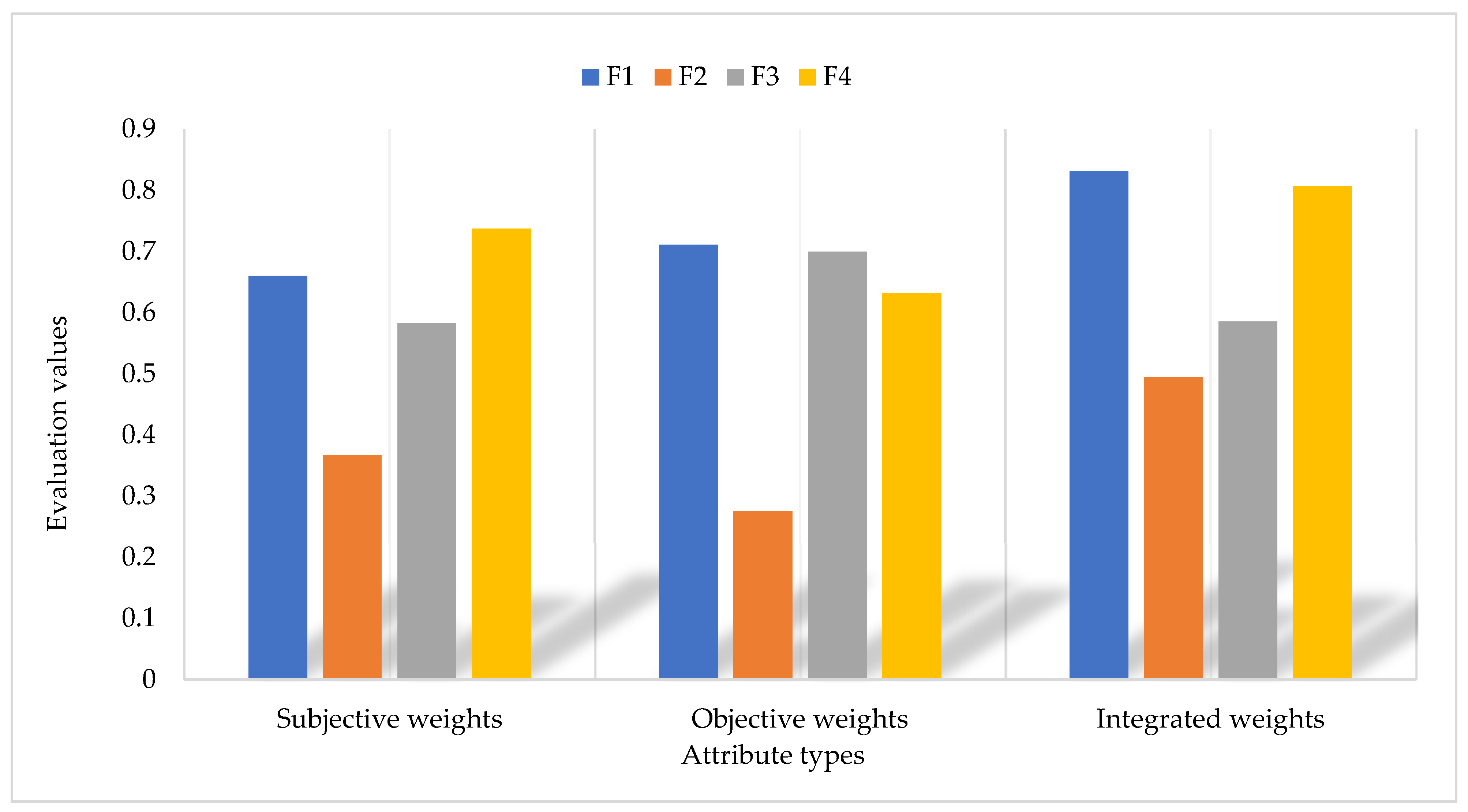
| Method | ||||||
|---|---|---|---|---|---|---|
| Subjective weights | 0.288 | 0.090 | 0.223 | 0.078 | 0.189 | 0.132 |
| Objective weights | 0.249 | 0.201 | 0.143 | 0.075 | 0.142 | 0.190 |
| Integrated weights | 0.400 | 0.100 | 0.178 | 0.033 | 0.150 | 0.140 |
| Ranking | ||||||
|---|---|---|---|---|---|---|
| 0.3104 | 0.3384 | 0.9620 | 0.7000 | 0.8310 | 1 | |
| 0.3192 | 1.1280 | 0.9890 | 0.0000 | 0.4945 | 4 | |
| 0.3227 | 0.0948 | 1.0000 | 0.1712 | 0.5856 | 3 | |
| 0.2864 | 0.3095 | 0.8875 | 0.7256 | 0.8066 | 2 |
| Ranking | ||||||
|---|---|---|---|---|---|---|
| 0.3055 | 0.4216 | 0.6524 | 0.6689 | 0.6607 | 2 | |
| 0.3432 | 1.2733 | 0.7330 | 0.0000 | 0.3665 | 4 | |
| 0.4682 | 1.0635 | 1.0000 | 0.1648 | 0.5824 | 3 | |
| 0.3427 | 0.3277 | 0.7319 | 0.7427 | 0.7373 | 1 |
| Ranking | ||||||
|---|---|---|---|---|---|---|
| 0.3115 | 0.2703 | 0.6118 | 0.8103 | 0.7111 | 1 | |
| 0.2808 | 1.4252 | 0.5516 | 0.0000 | 0.2758 | 4 | |
| 0.5091 | 1.8558 | 1.0000 | 0.3995 | 0.6998 | 2 | |
| 0.2512 | 0.3252 | 0.4935 | 0.7717 | 0.6326 | 3 |
| Ranking | |||||
|---|---|---|---|---|---|
| 0.7856 | 0.5000 | 0.4786 | 0.8019 | ||
| 0.8348 | 0.5033 | 0.5840 | 0.8152 | ||
| 0.8007 | 0.4551 | 0.5986 | 0.7804 | ||
| 0.7722 | 0.4186 | 0.6079 | 0.7558 | ||
| 0.7393 | 0.3778 | 0.6217 | 0.7266 | ||
| 0.7081 | 0.3380 | 0.6383 | 0.6974 | ||
| 0.6968 | 0.3228 | 0.6445 | 0.6862 | ||
| 0.6668 | 0.2822 | 0.6672 | 0.6582 | ||
| 0.6374 | 0.2446 | 0.6913 | 0.6309 |
| Proposed Integrated EDAS | VIKOR [27] | ARAS [27] | |||||||
|---|---|---|---|---|---|---|---|---|---|
| Ranking | Ranking | Ranking | |||||||
| 0.6607 | 2 | 0.2938 | 0.1834 | 0.1588 | 3 | 0.4487 | 0.7358 | 1 | |
| 0.3665 | 4 | 0.6155 | 0.2880 | 1.0000 | 1 | 0.2067 | 0.3389 | 4 | |
| 0.5824 | 3 | 0.5440 | 0.2230 | 0.7102 | 2 | 0.3141 | 0.5150 | 3 | |
| 0.7373 | 1 | 0.3005 | 0.1189 | 0.0121 | 4 | 0.4268 | 0.6998 | 2 | |
| TOPSIS [17] | WASPAS [26] | |||||||
|---|---|---|---|---|---|---|---|---|
| Ranking | Ranking | |||||||
| 0.1803 | 0.2249 | −0.0510 | 2 | 0.5380 | 0.4526 | 0.4953 | 1 | |
| 0.2013 | 0.2159 | −0.2103 | 3 | 0.3977 | 0.2817 | 0.3397 | 4 | |
| 0.2140 | 0.2046 | −0.3322 | 4 | 0.4580 | 0.2852 | 0.3716 | 3 | |
| 0.1750 | 0.2297 | 0.0000 | 1 | 0.5273 | 0.4613 | 0.4943 | 2 | |
| Established Model | [17] | [26] | [27] | [27] | |
|---|---|---|---|---|---|
| Ranking method | EDAS | TOPSIS | WASPAS | VIKOR | ARAS |
| Decision process | Group | Single | Group | Single | Single |
| Multiple aggregation strategies | Yes | No | No | No | No |
| DMs’ weights | Assumed | No | Computed | No | No |
| Criteria weights | Integrated | Assumed | Objective | Assumed | Assumed |
| Parameters involved | Yes | No | Yes | Yes | No |
Disclaimer/Publisher’s Note: The statements, opinions and data contained in all publications are solely those of the individual author(s) and contributor(s) and not of MDPI and/or the editor(s). MDPI and/or the editor(s) disclaim responsibility for any injury to people or property resulting from any ideas, methods, instructions or products referred to in the content. |
© 2023 by the authors. Licensee MDPI, Basel, Switzerland. This article is an open access article distributed under the terms and conditions of the Creative Commons Attribution (CC BY) license (https://creativecommons.org/licenses/by/4.0/).
Share and Cite
Zeng, S.; Chen, W.; Gu, J.; Zhang, E. An Integrated EDAS Model for Fermatean Fuzzy Multi-Attribute Group Decision Making and Its Application in Green-Supplier Selection. Systems 2023, 11, 162. https://doi.org/10.3390/systems11030162
Zeng S, Chen W, Gu J, Zhang E. An Integrated EDAS Model for Fermatean Fuzzy Multi-Attribute Group Decision Making and Its Application in Green-Supplier Selection. Systems. 2023; 11(3):162. https://doi.org/10.3390/systems11030162
Chicago/Turabian StyleZeng, Shouzhen, Wendi Chen, Jiaxing Gu, and Erhua Zhang. 2023. "An Integrated EDAS Model for Fermatean Fuzzy Multi-Attribute Group Decision Making and Its Application in Green-Supplier Selection" Systems 11, no. 3: 162. https://doi.org/10.3390/systems11030162