Article

The Strategic Weight Manipulation Model in Uncertain Environment: A Robust Risk Optimization Approach

1
School of Management Science and Engineering, Nanjing University of Information Science and Technology, Nanjing 210044, China
2
School of Management, Shanghai University, Shanghai 200444, China
3
Business School, University of Shanghai for Science and Technology, Shanghai 200093, China
*
Author to whom correspondence should be addressed.
Systems 2023, 11(3), 151; https://doi.org/10.3390/systems11030151
Submission received: 17 January 2023 / Revised: 9 March 2023 / Accepted: 14 March 2023 / Published: 15 March 2023
(This article belongs to the Topic Data-Driven Group Decision-Making)

Abstract

:
Due to the complexity and uncertainty of decision-making circumstances, it is difficult to provide an accurate compensation cost in strategic weight manipulation, making the compensation cost uncertain. Simultaneously, the change in the attribute weight is also accompanied by risk, which brings a greater challenge to manipulators’ decision making. However, few studies have investigated the risk aversion behavior of manipulators in uncertain circumstances. To address this research gap, a robust risk strategic weight manipulation approach is proposed in this paper. Firstly, mean-variance theory (MVT) was used to characterize manipulators’ risk preference behavior, and a risk strategic weight manipulation model was constructed. Secondly, the novel robust risk strategic weight manipulation model was developed based on the uncertainty caused by the estimation error of the mean and covariance matrix of the unit compensation cost. Finally, a case of emergency facility location was studied to verify the feasibility and effectiveness of the proposed method. The results of the sensitivity analysis and comparative analysis show that the proposed method can more accurately reflect manipulators’ risk preference behavior than the deterministic model. Meanwhile, some interesting conclusions are revealed.

1. Introduction

Multi-attribute decision making (MADM) is a process of investigating an alternative ranking under multiple attributes [1,2,3,4,5,6]. Identifying weights is an important challenge for MADM [7].To integrate the evaluation values of an alternative under multiple attributes, aggregation operators are often used by researchers [8,9]. In the development of human decision making, objective conditions such as technology [10,11,12,13,14,15] and decision-making information collection [16,17,18,19,20,21,22,23] no longer have the merit of dominating decision-making results. On the contrary, researchers have attached great importance to subjective conditions such as the motivation, decision consciousness, and knowledge level of decision makers. In other words, decision makers are strategic. Decision makers may express their opinion dishonestly to satisfy their interests [24], which will cause the decision results to develop in the direction they expect [25,26]. Therefore, it is meaningful to study strategic decision making.
In the real world, in order to realize their goal, decision makers will give a higher weight to specific attributes of an alternative, helping to achieve the expected ranking. This behavior is often referred to as strategic weight manipulation (SWM) [27]. Strategic decision making has been widely investigated by scholars. Dong et al. [28] investigated the strategic weight manipulation of multi-attribute decision making, and they reported that decision makers could strategically set attribute weights to achieve their desired alternative ranking. Liu et al. [29] indicated that attribute weights played a key role in alternative classification because different weights would lead to different alternative classification results. Dutta et al. [30] studied the TOPSIS multi-attribute decision-making approach for the case where the decision makers did not offer any weight information and provided partial weight preference information. Liu et al. [31] introduced strategic weight manipulation in interval attribute group decision making; they specified that the modification of the initial attribute weights needed to pay the cost, and they developed a linear programming model to optimize the cost. In the process of MADM, the allocation of attribute weights has a great influence on the scheme ranking [32,33]. Different weighting algorithms will obtain different sorting results when the criterion is weighted. For instance, the methods for calculating weights using AHP (analytic hierarchy process), BWM (Best Worst Method), and EWM (entropy weight method)—as well as the importance of the weight results—are all distinct. Although the pairwise comparison technique will yield inconsistent weight results, it is advantageous for risk preference decision makers. The weighting method of direct rating and distance estimation will provide consistent weights. Therefore, we acknowledge the varying importance of the weights in the different MADM approaches [34,35,36,37,38,39] that employ criteria weighting [40]. In different MADM methods, weights play different roles [41,42]. For example, expert weights can be dynamically generated from the MADM matrix. The attribute weight of entropy weight TOPSIS is improved by adjusting the weight coefficient, which improves the relative importance of attributes and reduces the impact of criteria with a large weight. In addition, different MADM methods consider different types of subjective or objective information. Because the objective weighting method ignores the decision makers’ experience, and the subjective weighting method ignores the performance ratings of alternatives across various criteria, objective and subjective weights must be combined in MADM.
In actual decision making, it is difficult to modify the weight, which needs to pay the corresponding cost. In SWM, the manipulator may use some resources (e.g., material, financial) to compensate the manager to achieve a specific ranking of the alternative, which is called the compensation cost. In strategic weight manipulation, each attribute weight modification has its corresponding unit compensation cost, which is often disturbed in the interval under an uncertain environment. In this paper, we abstractly represent the unit compensation cost corresponding to each attribute weight in vector form in order to quantitatively characterize the compensation cost. For more information, please refer to Example 1. The manipulator wants to spend as little of the cost as possible to achieve manipulation. However, decision makers are often in a complex and uncertain decision-making environment, where they do not have enough information and historical experience to determine how much compensation cost should be provided. Accordingly, the compensation cost of decision makers will be in a range rather than a fixed value.
In this paper, robust optimization is utilized to characterize the uncertainty of the compensation cost. Robust optimization is a powerful tool to tackle uncertain problems [43,44,45]. Different from stochastic programming [46,47] and fuzzy programming [48], robust optimization does not need to assume the probability distribution and fuzzy membership function of uncertain parameters but puts the uncertain parameters in an interval. The goal is to satisfy all implementations of the worst-case constraints [49,50]. In recent years, the robust optimization approach has been widely used in consensus-reaching processes [51], portfolios [52], location allocation [53], and other fields. However, few scholars have applied robust optimization to strategic weight manipulation. For example, Jin et al. [54] found that an uncertain unit adjustment cost would lead to a higher weight allocation cost, and they illustrated the effectiveness of their proposed model through an actual anti-epidemic case. We note that the method proposed in this paper is different from theirs, which only investigated the uncertain unit compensation cost. Ji et al. [55] discussed the expected ranking of alternatives under uncertain attribute values, and they pointed out that attribute weights were easier to manipulate when attribute values obeyed a linear uncertain distribution.
Uncertain circumstances in decision making are often accompanied by risks [56], which cannot be completely eliminated. To describe the risks faced by the manipulator in an uncertain environment, we introduce the concept of the risk-sensitive cost. The risk cost refers to the expenses that people must pay due to the existence of risk. Decision risk is present in SWM under uncertain settings. The quality of the model and the outcomes of the solutions will suffer if the decision risk is not taken into account. As a result, MVT is utilized to describe the risk of the compensation cost. In other words, the cost vector’s mean or covariance matrix contains the estimation error, which poses a risk. Hence, this paper reflects the risk cost by discussing the disturbance of the mean or covariance. For more information, please refer to Example 2. The optimal decision scheme of the manipulator is to minimize the compensation cost and reduce the impact of the risk-sensitive cost [57,58]. To measure the risk-sensitive cost, we need to use risk measurement tools in decision making. Risk measurement methods mainly include mean-variance theory [59], conditional value at risk [60,61,62], and the Von Neumann–Morgenstern utility measure [63]. MVT has a straightforward solution technique that can yield realistic and practical solutions. Consequently, this paper describes the risk compensation cost of the manipulator through mean-variance theory.
The literature review mentioned above reveals that the current SWM issue has a lot of flaws. For instance, there will be risks associated with the SWM problem in an uncertain environment that cannot be entirely eradicated. The best decision-making strategy should aim to cut costs and lessen risky outcomes. In order to achieve the least risk-sensitive cost, this paper first proposes a risk strategic weight manipulation (rSWM) based on MVT. Because minimax rSWM (Robust rSWM) is more suited to uncertain decision environments, it is the model we recommend. The proposed robust rSWM offers a solution to address the ambiguity and estimation error of the mean and covariance, two parameters connected to the uncertain unit adjustment cost. A set is used to describe the mean and covariance uncertainty.
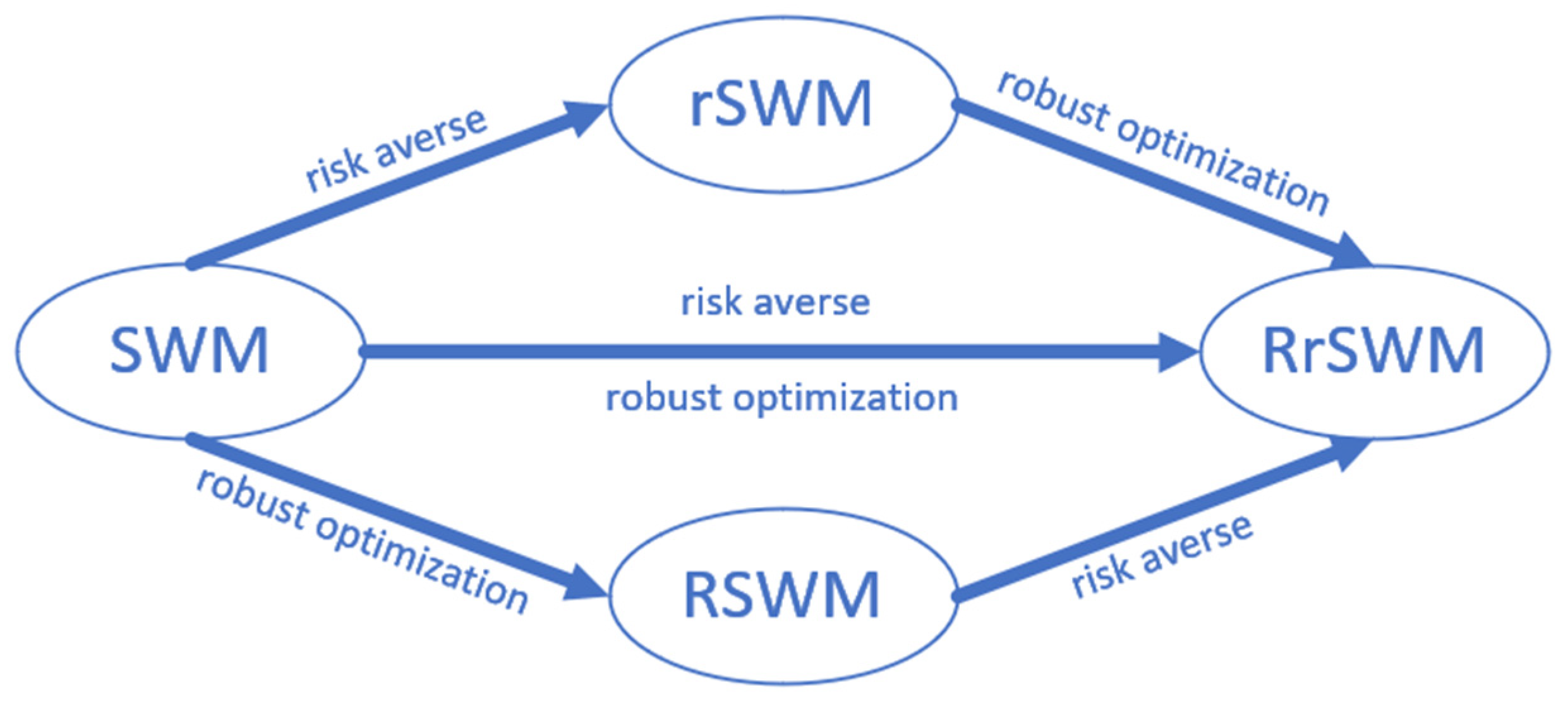
The contributions of this paper are summarized as follows: (1) Compared with the deterministic compensation cost, the uncertain cost is characterized by the robust optimization method in this paper. (2) In this paper, some errors in calculating the mean and variance of the unit compensation cost are considered, and the risk aversion behavior of the manipulator is described using MVT. A risk-averse robust strategic weight manipulation model (RrSWM) is built, which is equivalently transformed into a tractable robust counterpart model through duality theory. Meanwhile, the proposed model is an extension of the robust strategic weight manipulation model (RSWM). To establish a connection with the extant strategic weight manipulation models, the specific transformation conditions between them are given. (3) Through a practical application of emergency facility location, the applicability of the proposed model is covered. The approach in this paper is more effective than prevenient methods, which is shown through comparative analysis and sensitivity analysis. Our work can provide some reference for the government or enterprises to carry out risk management.
The remainder of this paper is organized as follows: Section 2 presents some basic knowledge utilized in this paper; Section 3 proposes a robust risk strategic weight manipulation model; Section 4 specifies a case study and presents the comparative analysis and sensitivity analysis; Section 5 concludes this paper and puts forward future research work.

2. Preliminaries

In order to assist the readers in understanding the proposed approach, some preliminaries are introduced in this section. Several approaches, theories, and models of strategic weight manipulation and robust optimization are presented.

2.1. Strategic Weight Manipulation

We define X = x 1 , x 2 , x m as a set of alternatives. A = a 1 , a 2 , a n is a set of multiple attributes. ω = ω 1 , ω 2 , ω n is the weight set corresponding to the attribute, where ω j 0 and j = 1 n ω j = 1 . We assume I = 1 , 2 , m and J = 1 , 2 , n are number sets. Therefore, the decision matrix is S = s i j m × n , where s i j indicates the attributes value of an alternative x i X with respect to a j A .
Generally speaking, multi-attribute decision making is divided into three sections: normalization of the decision matrix, aggregation of the standardized decision matrix, and ranking of alternatives.
(1) Normalization of decision matrix
For benefit indicators, the standardized process is shown in Equation (1):
r i j = s i j min ( s i j ) i max ( s i j ) i min ( s i j ) i .
For cost indicators, the standardized process is shown in Equation (2):
r i j = max ( s i j ) i s i j max ( s i j ) i min ( s i j ) i .
(2) Aggregation of the standardized decision matrix
Assume D ( x i ) is the comprehensive evaluation score of the alternative x i under various attributes, which can be calculated by introducing the aggregation function. The weighted average (WA) and ordered weighted average (OWA) operators are the most often used aggregation operators. In this work, we utilize the WA operator to compute the comprehensive evaluation score of alternatives, as shown in Equation (3):
D ( x i ) = W A ω ( r i 1 , r i 2 , , r i n ) = j = 1 n ω j r i j .
(3) Ranking of alternatives
The ranking order is determined by comparing the score D ( x i ) of alternative x i , which ranks first with the higher value. When comparing the ranking of alternatives x i , ( i I ) and x l , ( l I ) , in order to calculate the ranking of alternative x l , we only need to find out the number of alternatives that meet the cardinality set H = x l D ( x i ) > D ( x l ) , ( i l ) . Suppose p ( x l ) represents the ranking of alternative x l ; therefore, we have p ( x l ) = H + 1 .
In multi-attribute decision making, the attribute weights will be manipulated strategically by decision makers to realize their interests. Assuming that the manipulator wants to change the ranking of alternative x l , we define the expected ranking of the manipulator as p ( x l ) ; it is obvious that p ( x l ) = p ( x l ) . Suppose the attribute weight vector before manipulation is ω 0 = ( ω 1 0 , ω 2 0 , ω n 0 ) T , the weight vector after manipulation is ω = ( ω 1 , ω 2 , ω n ) T , and the attribute weight deviation in the manipulation process is d j = ω j 0 ω j . Assuming that the unit compensation cost is c j , the total cost paid by the decision makers to manipulate the attribute weight is c T d . We introduce an infinite constant M and a binary variable y i l .
In order to comprehensively treat the compensation cost, we propose an example to illustrate it.
Example 1.
Suppose the vector of the compensation cost is c = [ 3 , 2 , 4 , 5 , 2.5 ] , and the unit compensation cost corresponding to each attribute is 3, 2, 4, 5, and 2.5, respectively. The weight adjustment deviation is d = [ d 1 , d 2 , d 3 , d 4 , d 5 ] ; therefore, we can obtain the total cost c T d that the decision maker should pay.
The manipulator wants to make the compensation cost as low as possible. Hence, the minimum cost strategic weight manipulation model built in this paper is as follows:
min c T d s . t . j = 1 n ω j r i j > j = 1 n ω j r l j ( 1 y i l ) M , i I j = 1 n ω j r i j j = 1 n ω j r l j + y i l M , i I i = 1 , i l m y i l + 1 = p ( x l ) , l I ω j 0 ω j d j , j J j = 1 n ω j = 1 , j J y i l 0 , 1 , i I , l I 0 ω j 1 , j J
The objective function is to minimize the total cost to be compensated by the manipulator to change the attribute weight. The specific constraints are as follows. The first constraint and the second constraint represent the comprehensive evaluation score comparison between alternatives x i , ( i I ) and x l , ( l I ) . We introduce an infinite constant M and a binary variable y i l in model (4). When y i l = 1 , we have D ( x i ) > D ( x l ) . On the contrary, when y i l = 0 , we have D ( x i ) D ( x l ) . The third constraint represents the expected ranking of alternative x l . The fourth constraint indicates that the attribute a j weight deviation in the manipulation process is less than or equal to d j . The fifth constraint indicates that the sum of attribute weights is 1. The sixth constraint is the binary variable. The seventh constraint indicates that the weight of attribute a j is greater than 0 but not greater than 1.

2.2. Robust Optimization

Uncertainty exists extensively in MADM. For example, the compensation cost of SWM in real life is often uncertain, because the manipulator cannot know the probability distribution information of the compensation cost in advance. Therefore, this paper utilizes robust optimization to deal with the uncertainty of the parameters. The key to robust optimization is to select an appropriate uncertainty set to characterize the random parameters and meet the realization of all constraints in the worst case.
We first introduce a general linear programming problem:
min c T d s . t . c T d H A d h  
where the variable c is the given data, d n is the decision variable vector, A m × n is the coefficient matrix of the uncertain parameters, and h m is the right-hand-side vector. When the uncertain parameters fluctuate in the uncertainty set U , the robust optimization model can be expressed as
min c T d s . t . c T d H A d h A , h U
The perturbation vector ζ changes in the form of an affine transformation in a given perturbation set Z , which is expressed as follows:
U = [ a i ; h i ] = [ a i 0 ; h i 0 ] + b = 1 B ζ b   [ a i b ; h i b ] : ζ Z
where a i denotes the i - t h row of matrix A , and h i denotes the i - t h element of vector h .
Assume a i T d h i is the i - t h constraint in A d h . We let a i = a i 0 + b = 1 B ζ b a i b and h i = h i 0 + b = 1 B ζ b h i b , where a i 0 and h i 0 are the nominal values of the uncertain parameters, a i b and h i b are basic shifts. In order to control the range of uncertainty, the new variable ζ is introduced. Hence, the inequality can also be written as
a i 0 d + b = 1 B ζ b a i b d h i 0 + b = 1 B ζ b h i b .
Then, the robust counterpart of model (6) can be expressed as
min c T d s . t . c T d H   a i 0 d + sup ζ   Z b = 1 B ζ b a i b d ζ b h i b h i 0
The feasible solution and optimal value of model (6) are equivalent to the feasible solution and optimal value of model (9). Because model (9) is a semi-infinite programming problem, it is difficult to solve it in polynomial time. In this paper, we equivalently transform model (9) into convex optimization problems under different scenarios.

3. The Proposed Model

Previous studies investigated the uncertainty of the compensation cost in SWM. However, the risk preference of decision makers was not taken into account. The uncertainty of decision making is often accompanied by risk. The lowest cost and the lowest risk are expected by decision makers. Accordingly, we introduce the risk function to describe the risk associated with decision making. It is assumed that the compensation cost c is a random parameter with a mean value α and variance β = E ( c α ) ( c α ) T . The risk aversion cost of the manipulator is E ( c T d ) + λ v a r   ( c T d ) , where E ( c T d ) = α T d represents the expected cost that the manipulator needs to compensate for adjusting the attribute weight of the alternative, and v a r   ( c T d ) = d T β d stands for the variance of the cost. λ 0 indicates the risk aversion coefficient of the manipulator. Generally speaking, with the increase in the value of λ , the risk aversion degree of the manipulator gradually increases.
In order to comprehensively treat the risk-sensitive cost, an example is proposed.
Example 2.
Suppose the evaluation value of the compensation cost is a matrix C = [ c i j ] 10 × 5 . We can obtain the mean value α = [ m 1 , m 2 , m 3 , m 4 , m 5 ] and covariance matrix β = [ cov i j ] 5 × 5 using the MATLAB tool. The weight adjustment deviation is d = [ d 1 , d 2 , d 3 , d 4 , d 5 ] ; therefore, we can obtain the total risk cost α T d + λ d T β d that the decision maker should pay. λ is the risk aversion coefficient.
Therefore, the model with risk aversion (rSWM) constructed in this paper is as follows. We define model (10) as model D1:
min α T d + λ · d T β d s . t . j = 1 n ω j r i j > j = 1 n ω j r l j ( 1 y i l ) M , i I j = 1 n ω j r i j j = 1 n ω j r l j + y i l M , i I i = 1 , i l m y i l + 1 = p x l , l I ω j 0 ω j d j , j J j = 1 n ω j = 1 , j J y i l 0 , 1 , i I , l I 0 ω j 1 , j J
The objective function includes the risk aversion behavior of the manipulator, including the mean value and covariance of the compensation cost. The objective is to minimize the sum of the mean value and covariance evaluation errors. The details of the constraints are as follows. The first constraint and the second constraint represent the comprehensive evaluation score comparison between alternatives x i , ( i I ) and x l , ( l I ) . An infinite constant M and a binary variable y i l are introduced here. When y i l = 1 , we have D ( x i ) > D ( x l ) . On the contrary, when y i l = 0 , we have D ( x i ) D ( x l ) . The third constraint represents the expected ranking of alternative x l for the manipulator. The fourth constraint indicates that the attribute a j weight deviation is less than or equal to d j . The fifth constraint indicates that the sum of attribute weights is 1. The sixth constraint is the binary variable. The seventh constraint indicates that the weight of attribute a j is greater than 0 but not greater than 1.
However, the cost change caused by the evaluation error of the cost mean and variance cannot be sufficiently measured with the above model. The robustness of model D1 is poor. Therefore, we characterize the perturbation of the cost mean and variance through robust optimization. We discuss the minimum cost incurred by the manipulator in three cases: in the first case, we research the uncertain risk of the cost mean when the cost variance is known; in the second case, we investigate the uncertain risk of the cost variance when the cost mean is known; in the third case, we discuss the uncertain risk when the evaluation errors of cost mean and covariance are both present.

3.1. The Mean Value of the Compensation Cost Is Uncertain

When the covariance of the unit compensation cost is known, we may compute the minimum risk-sensitive cost under the given uncertainty set U = α = α 0 + b = 1 B ζ b α b : ζ Z . The model we constructed is as follows:
min   d , ω j sup α U α T d + λ · d T β d s . t . j = 1 n ω j r i j > j = 1 n ω j r l j ( 1 y i l ) M , i I j = 1 n ω j r i j j = 1 n ω j r l j + y i l M , i I i = 1 , i l m y i l + 1 = p x l , l I ω j 0 ω j d j , j J j = 1 n ω j = 1 , j J y i l 0 , 1 , i I , l I     0 ω j 1 , j J
Because the goal function involves an operator min sup , model (11) cannot be solved directly. When the mean value of the unit compensation cost is uncertain, we characterize the perturbation of the cost using two commonly used uncertainty sets in robust optimization, namely, a box set and an ellipsoid set.

3.1.1. Box Uncertainty Set

Theorem 1.
If the mean value of the uncertain cost is defined as a box uncertainty set, that is, Z b o x = ζ R B : ζ Ψ , where Ψ is the level of parameter uncertainty, the robust counterpart of model (11) can be constructed as model (12). We define model (12) as P1.
min   d , ω j α 0 T d + Ψ b = 1 B α b T d + λ · d T β d s . t . j = 1 n ω j r i j > j = 1 n ω j r l j ( 1 y i l ) M , i I j = 1 n ω j r i j j = 1 n ω j r l j + y i l M , i I i = 1 , i l m y i l + 1 = p x l , l I ω j 0 ω j d j , j J j = 1 n ω j = 1 , j J y i l 0 , 1 , i I , l I     0 ω j 1 , j J
Proof of Theorem 1.
[64] According to the definition of the box set, the uncertain cost to be compensated by the risk manipulator can be written as
α 0 T d + b = 1 B ζ b α b T d + λ d T β d H , ( ζ R B : ζ Ψ ) .
Then, we can obtain
b = 1 B ζ b α b T d H α 0 T d λ d T β d , ( ζ R B : ζ Ψ ) .
In the worst case, we have
max ζ Ψ b = 1 B ζ b α b T d H α 0 T d λ d T β d .
Because the maximum value on the left side of the inequality is Ψ b = 1 B α b T d , the explicit constraint form can be obtained:
α 0 T d + Ψ b = 1 B α b T d + λ d T β d H .
As a result, the box uncertainty set model is proven. □

3.1.2. Ellipsoid Uncertainty Set

Theorem 2.
If the mean value of the uncertain cost is defined as an ellipsoid uncertainty set, that is, Z e l l i p s o i d = ζ R B : ζ 2 Ω , where Ω is the level of parameter uncertainty, the robust counterpart of model (11) can be built as model (13). We define model (13) as P2.
min   d , ω j α 0 T d + Ω b = 1 B ( α b T d ) 2 + λ · d T β d s . t . j = 1 n ω j r i j > j = 1 n ω j r l j ( 1 y i l ) M , i I j = 1 n ω j r i j j = 1 n ω j r l j + y i l M , i I i = 1 , i l m y i l + 1 = p x l , l I ω j 0 ω j d j , j J j = 1 n ω j = 1 , j J y i l 0 , 1 , i I , l I     0 ω j 1 , j J
Proof of Theorem 2.
[65] According to the definition of the ellipsoid set, the uncertain cost to be compensated by the risk manipulator can be written as
α 0 T d + b = 1 B ζ b α b T d + λ d T β d H , ( ζ R B : ζ 2 Ω ) .
Then, we can obtain
b = 1 B ζ b α b T d H α 0 T d λ d T β d , ( ζ R B : ζ 2 Ω ) .
In the worst case, we have
max ζ 2 Ω b = 1 B ζ b α b T d H α 0 T d λ d T β d .
Consequently, the explicit form of the above formula can be obtained:
α 0 T d + Ω b = 1 B ( α b T d ) 2 + λ d T β d H .
Therefore, the model based on the ellipsoid uncertainty set is proved. □

3.2. The Compensation Cost Covariance Matrix Is Uncertain

When the mean value of the unit compensation cost is known, we can compute the minimum risk-sensitive cost under the provided uncertainty set regarding the covariance of the unit compensation cost. The model we constructed is as follows:
min   d , ω j sup β Γ α T d + λ · d T β d s . t . j = 1 n ω j r i j > j = 1 n ω j r l j ( 1 y i l ) M , i I j = 1 n ω j r i j j = 1 n ω j r l j + y i l M , i I i = 1 , i l m y i l + 1 = p x l , l I ω j 0 ω j d j , j J j = 1 n ω j = 1 , j J y i l 0 , 1 , i I , l I     0 ω j 1 , j J
where Γ is an uncertainty set provided in advance.
The simplest way to describe the uncertainty set Γ is to add a set of interval positivity constraints: Γ = β 0 ξ β ξ + , where ξ and ξ + are the lower and upper limits of β , which are positive semidefinite matrices.
Theorem 3.
When the evaluation error of the cost variance change in the set of uncertainty intervals Γ = β 0 ξ β ξ + , model (14) is equivalently transformed into model (15). We define model (15) as P3.
min   d , ω j α T d + λ · d T ξ + d s . t . j = 1 n ω j r i j > j = 1 n ω j r l j ( 1 y i l ) M , i I j = 1 n ω j r i j j = 1 n ω j r l j + y i l M , i I i = 1 , i l m y i l + 1 = p x l , l I ω j 0 ω j d j , j J j = 1 n ω j = 1 , j J y i l 0 , 1 , i I , l I     0 ω j 1 , j J
Proof of Theorem 3.
[59] The internal maximization problem of model (14) is
max β α T d + λ d T β d s . t . ξ β ξ + β 0
when β 0 is not considered, for all i , d i 0 , we have d i d j 0 . When all β i j take the upper bound value—that is, β i j = ξ i j + —the relaxation problem d T β d = i , j d i β d j of model (16) reaches the maximum value. Because ξ + is assumed to be a positive semidefinite matrix, it must be optimum for the non-relaxation model (16). The proof is finished. □

3.3. Both the Mean Value and Compensation Cost Covariance Matrix Are Uncertain

In this section, we introduce the interval uncertainty sets U = α 0 μ α μ + and Γ = β 0 ξ β ξ + to characterize the perturbations of the mean value and covariance matrix of the unit compensation cost. μ , μ + , ξ , and ξ + represent the lower and upper bounds of α and β , respectively. ξ and ξ + are positive semidefinite matrices. A new model is constructed as follows:
min   d , ω j sup α U , β Γ α T d + λ · d T β d s . t . j = 1 n ω j r i j > j = 1 n ω j r l j ( 1 y i l ) M , i I j = 1 n ω j r i j j = 1 n ω j r l j + y i l M , i I i = 1 , i l m y i l + 1 = p x l , l I ω j 0 ω j d j , j J j = 1 n ω j = 1 , j J y i l 0 , 1 , i I , l I     0 ω j 1 , j J
where U and Γ are the given uncertainty sets.
Theorem 4.
When the mean value and covariance of the unit compensation cost change in the uncertainty intervals U = α 0 μ α μ + and Γ = β 0 ξ β ξ + , model (17) is equivalently transformed into model (18). We define model (18) as P4.
min   d , ω j μ + T d + λ · d T ξ + d s . t . j = 1 n ω j r i j > j = 1 n ω j r l j ( 1 y i l ) M , i I j = 1 n ω j r i j j = 1 n ω j r l j + y i l M , i I i = 1 , i l m y i l + 1 = p x l , l I ω j 0 ω j d j , j J j = 1 n ω j = 1 , j J y i l 0 , 1 , i I , l I     0 ω j 1 , j J
Proof of Theorem 4.
[59] Because the internal maximizing issue of model (17) is divisible, it may be separated into two maximization problems: max α U α T d and max β Γ d T β d . For the first maximization problem:
max α U α T d s . t . μ α μ +
Because d 0 , when each vector element takes its upper bound—that is, α = μ + —the maximum value is obtained by the objective function in model (19). The proof of the procedure for the second maximizing issue is identical to that of Theorem 3. □

4. Case Simulation

This section verifies the RrSWM proposed in Section 3 using specific examples. Additionally, sensitivity analysis and comparative analysis are carried out to demonstrate the merits of the proposed models.

4.1. Case Study

A case is utilized to illustrate the feasibility of the proposed model in this section. All the necessary codes were run in MATLAB R2016a on a MacBook Air 2019 (1.6 GHz Intel Core i5), coupled with the CPLEX solver and YALMIP toolbox.
Since the beginning of COVID-19 in 2019, millions of people around the world have been infected, which has caused huge losses to the economy and society of each country and region. In order to effectively block the social transmission of the pandemic in a timely manner, resolute measures have been taken by the Chinese government to establish a number of module hospitals (MHs) to treat people with mild infection or isolate close contacts. MHs are modular healthcare facilities, with the functions of emergency treatment and surgical procedures. They have the merits of good mobility, rapid deployment, and strong environmental adaptability. Hence, they are widely utilized in emergency medical rescue tasks. After the outbreak of the pandemic, understanding how to choose the location of MHs to ensure that patients are treated timely and effectively was a great test for the urban emergency management system.
Considering the emergency facility location of MHs during COVID-19, we assumed that x 1 , x 2 , , x 9 , x 10 are ten candidate locations of MHs, and we chose three of them to better serve patients. a 1 , a 2 , a 3 , a 4 , a 5 represents the number of infected people, the number of medical staff, the facility infrastructure of MHs (beds), the average relative position of the infected people’s residence (kilometers), and the time taken for the construction of MHs (hours), respectively. a 1 , a 4 , and a 5 are cost indicators, and a 2 and a 3 are benefit indicators. The data desired in this paper are shown in Table 1.
We standardized the data in Table 1 through Equations (1) and (2) to obtain a standardized decision matrix, as shown in Table 2. Then, we assumed that the initial weight vector of the five attributes is ω 0 = ( 0.2 , 0.2 , 0.2 , 0.2 , 0.2 ) T , B = 3 . Simultaneously, we assumed that the uncertain parameters are Ψ = 1 and Ω = 1 . Assuming the compensation cost is a random variable, the mean value is α = ( 2.3   3.0   3.1   1.7   2.5 ) , and the covariance matrix is as follows:
β = 1.6603 0.1339 0.1397 0.3489 0.4533 0.1339 1.0846 0.3261 0.1722 0.4477 0.1397 0.3261 0.9668 0.4481 0.0953 0.3489 0.1722 0.4481 1.0727 0.7202 0.4533 0.4477 0.0953 0.7202 2.5967 .
As a result of α = α 0 + b = 1 3 α b ζ , we let α 0 = α ; that is, α 0 = ( 2.3   3.0   3.1   1.7   2.5 ) . α b is a basic shift coefficient matrix, as follows:
α b = 0.20 0.16 0.25 0.37 0.15 0.20 0.27 0.14 0.09 0.24 0.25 0.15 0.14 0.09 0.26 .
In order not to lose generality, we assumed that the risk aversion coefficient of the manipulator is λ = 10 , α + = 1.2 α 0 , ξ + = 1.3 β .
The actual emergency decision-making environment is full of uncertain factors, and the manipulator has to pay higher compensation costs in order to ensure the stability of the location decisions. To illustrate this fact through numerical simulation, the calculation results of the proposed model for when the ranking of x 8 is equal to 2, for instance, are shown in Table 3.
As we can see in Table 3, the cost of model D1 is lower than that of model P1 to model P4, which is in line with the actual location decision. However, the optimal value of model P2 is closer to the rSWM model. In other words, the decision maker incurs the lowest cost when the ellipsoid uncertainty set is utilized to describe the risk cost. In addition, model P1 to model P4 take into account the manipulator’s risk-averse behavior, so the decision results are also conservative. The above analysis results verify the applicability of the proposed model.
The following Table 4 shows the running time of the computer in solving the model. As we can see, the solution time of the five models is relatively short, with the longest time not exceeding 0.5 s. Therefore, the model proposed in this paper is suitable for emergency facility location decisions.

4.2. Model Discussion

In this section, firstly, sensitivity analysis is performed to specify some parameters that affect the model to reveal how the uncertain factors affect the manipulator’s decision making. Then, the relationship between the proposed model and the extant strategic weight manipulation model is discussed. Finally, comparative analysis is performed between the proposed method and the existing strategic weight manipulation approaches.

4.2.1. Sensitivity Analysis

In strategic weight manipulation, the behavior of the manipulator will be affected by some uncertain parameters, and sensitivity analysis is often utilized to explore the impact of parameter fluctuations on the proposed model results [66]. The data in Section 4 are also used here. The key parameters in this paper are the manipulator’s risk aversion coefficient λ , nominal value α 0 , basic shift coefficient matrix α b , covariance matrix β , and uncertain level parameters ζ . We keep the other parameters constant.
(1) The impact of the risk aversion coefficient λ on D1
The influence of the manipulator’s risk aversion coefficient on the minimal compensation cost is interesting to examine. As shown in Figure 1, under the condition of keeping the other parameters constant, the compensation cost of the manipulator gradually increases with the increase in the risk aversion coefficient. This means that increasing the value of risk factors within a certain range will have a significant impact on the cost for the manipulator to set strategic weights. In other words, the risk factors in decision making will increase the cost of decision making. Manipulators should master more comprehensive information to reduce the uncertainty and risk in decision making. For the problems in actual circumstances, we should control the variability in the parameters within an acceptable range.
(2) The effect of the nominal value α 0 on D1, P1, and P2
The perturbation of the nominal value α 0 can affect the compensation cost of the manipulator and the attribute weight value. With the other conditions unchanged, the analysis results of different nominal values are shown in Figure 2. With the increase in the nominal value α 0 , the compensation cost of the manipulator increases gradually. It is found that the minimum compensation cost of model P1 and model P2 is basically consistent with the rSWM model under the same nominal value. It is also found that the change in the nominal value will increase the compensation cost. However, it is not sensitive to different models.
In addition, the influence of α 0 ± 0.2 on the attribute weight and minimum cost was investigated, as shown in Table 5. When an α 0 of 0.2 is added, the minimum compensation cost of the manipulator increases from 3.1701 to 3.3162. The rSWM model does not take into account the uncertainty in the decision-making environment. However, when we use the robust optimization approach to characterize the uncertain mean value of the compensation cost, the optimal values of models P1 and P2 are sufficient to meet the aim of strategic weight manipulation.
(3) The effect of a basic shift on P1 and P2
The coefficient matrix is a small disturbance of the cost mean based on the nominal value α 0 . For the sake of researching the influence of the coefficient matrix α b on the manipulator’s compensation cost, we utilized Monte Carlo simulation to randomly generate 300 novel data sets. The 300 data sets were divided into 15 groups as the input parameters of models P1 and P2, so as to solve the minimum compensation cost. Then, the average value of each group was taken as the final cost result. The data analysis results are shown in Figure 3.
As can be seen in Figure 3, with the perturbation of the basic shift, the minimum compensation cost of the manipulator also changes. However, the cost value is generally distributed around a certain value. For example, the cost value of model P1 is distributed around 3.26. The minimum cost value of model P2 is smaller than that of model P1. In other words, the ellipsoid uncertainty set model, which measures the manipulator’s compensation cost, is less conservative.
(4) The impact of the covariance matrix β on D1 and P3
The influence of the covariance matrix β on the minimum compensation cost of the manipulator is worth studying. Table 6 shows the data analysis findings assuming that the covariance matrix changes from 0.7 β to 1.2 β .
It can be seen in Table 6 that with the increase in the covariance matrix, the compensation cost of the manipulator increases. In model P3, when the covariance matrix is greater than or equal to β , the weight of attribute two is 0. When the covariance matrix increases from β to 1.2 β , the compensation cost of D1 changes from 3.1701 to 3.4245. With the increase in the covariance matrix, the compensation cost changes slightly. In order to achieve their own goals, the manipulator must be able to afford certain compensation costs. The compensation cost of model P3 is higher than that of D1. If the uncertainty of the covariance matrix in model P3 is not considered, the solution of model D1 cannot reflect the risk and uncertainty in strategic weight manipulation.
(5) The effect of uncertain level parameters on P1 and P2
It is worth investigating the impact of different uncertain level parameters on the manipulator’s compensation cost. Suppose the following three alternatives are manipulated: x 3 , x 6 , and x 8 , with ranks of 2. Assuming that Ψ and Ω increase from 1 to 6, the other parameters remain constant. The data results are shown in Figure 4 and Figure 5. In models P1 and P2, with the increase in uncertain level parameters, the minimum compensation cost of the manipulator increases. However, alternative x 3 is less affected by the perturbation of the uncertain level parameters. The manipulator can achieve their goal without paying a certain cost, so the ranking of alternative x 3 can easily be manipulated. The manipulation cost of alternative x 6 changes rapidly with the uncertain parameters, and its robustness is superior. Additionally, it is hard for the manipulator to change the ranking of alternative x 6 .

4.2.2. Relationships between the RrSWM and Extant Models

In order to investigate the relationships between the proposed model and the extant strategic weight manipulation models, a relationship diagram of several models was constructed, as shown in Figure 6. As stated in Section 3, under the risk aversion behavior of the manipulator, the SWM model is transformed into the rSWM model. When the uncertain factors in decision making are considered, the SWM model is converted to the RSWM model through the robust optimization method. By considering the uncertain factors in the rSWM model, it can be transformed into the RrSWM model. When the risk measure function is added to the RSWM model, we obtain the RrSWM model.

4.2.3. Comparative Analysis

This paper compares the proposed method with the extant strategic weight manipulation approaches to illustrate the merits of the proposed method.
(1) Comparing Dong et al.’s model [28] with our work from the perspective of whether the manipulator compensates the cost
The optimization goal of the SWM model proposed by Dong et al. is to minimize the sum of the weight deviation. However, the cost of weight manipulation is not considered in Dong et al.’s work. We utilized the data in Section 4, and the results are shown in Table 7.
It can be seen in Table 7 that the sum of the attribute weights’ adjusted deviation in this paper is 0.7311, which is higher than that of the SWM model proposed in Dong et al.’s work. However, combined with the emergency facility location problems, there are many uncertain factors in the MH facility locations, and the manipulator has to compensate certain risk costs. The cost uncertainty and manipulator’s risk behavior are considered in this paper, which is more practical than the deterministic model in MADM.
(2) Comparing Jin et al.’s model [54] with our work from the perspective of the strategic weight manipulation of the uncertain unit compensation cost
In strategic weight manipulation, the manipulator evaluates the compensation cost according to the change in the expected ranking of alternatives. Jin et al. researched the uncertainty of the compensation cost in strategic weight manipulation through the robust optimization method. The risk mentality of the manipulator, however, was not taken into account in Jin et al.’s method. Accordingly, we verified the advantages of the proposed method by comparing the experimental results of the two methods. Ten groups of random data were generated, which were input into the model of this paper and Jin et al.’s model. The data comparison results are shown in Table 8.
It can be seen from the data in Table 8 that the weight setting of the proposed method is relatively reasonable without a certain attribute weight being too large. When the risk attitude of the manipulator is considered in the RrSWM model, reasonable attribute weight distribution results can be acquired at a greater compensation cost. When the manipulator is confronted with ambiguous decision-making circumstances, they will provide a more relaxed mode to realize their goal because of the existence of risk. Therefore, greater costs will be compensated by the manipulator. Decision making in reality is similar to this.

5. Conclusions and Future Work

The SWM model focuses on MADM under complete information. However, in practice, the manipulator needs to compensate for a certain cost in order to achieve their desired ranking of alternatives. Due to the complexity and uncertainty of decision-making circumstances, the manipulator’s compensation cost is difficult to measure accurately. Simultaneously, the uncertainty of the decision-making environment is accompanied by a risk cost. In this paper, an RrSWM model is proposed to solve the above issues. The strategic weight manipulation behavior of risk aversion in three cases was investigated using MVT. The impact of the mean value change of the unit compensation cost on the minimum compensation cost and weight setting was investigated for when the cost covariance of the unit compensation cost was known in advance. Similarly, the impact of the covariance change of the unit compensation cost on the minimum compensation cost and weight setting was studied for when the cost mean of the unit compensation cost was known in advance. Further, the impact on the minimum compensation cost and weight setting was researched for when the cost mean and covariance were unknown. Finally, the effectiveness of the proposed model was verified by a case of emergency facility location. The following are some intriguing conclusions:
(1)
The risk behavior of the manipulator has a substantial influence on the decision outcomes. The manipulator will incur higher compensation expenses as their risk aversion level rises. Similarly, the increase in uncertain level parameters will also cause the manipulator to pay a greater compensation cost. However, the effect of the basic shift on the compensation cost of models P1 and P2 is different from the other parameters, and it converges near a certain value;
(2)
There is a certain conditional transformation relationship between the model proposed in this paper and the extant SWM models. The robust optimization method and risk function are the sources of the transformation;
(3)
Compared with the risk-neutral strategic weight manipulation problem, the uncertain factors and risk factors are fully considered in the proposed method, and we obtained a more reasonable attribute weight setting result in the case simulation.
With the development of information technology and the advent of the big data era, the sources of decision-making information are becoming more abundant [67]. Understanding how to make good use of this information to guide decision making is a big challenge. Based on this, a data-driven robust optimization method can be constructed to investigate the risk-averse strategic weight manipulation behavior of the manipulator in uncertain circumstances. Another meaningful research direction is to choose other forms of uncertainty sets to research the impact of the manipulator’s risk aversion behavior on the minimum compensation cost.

Author Contributions

Conceptualization, Y.J., L.W. and S.Q.; data curation, L.W. and L.Z.; formal analysis, Y.J. and L.Z.; investigation, L.W., S.Q. and Z.W.; methodology, Y.J., L.W. and S.Q.; resources, Y.J., L.W. and Z.W.; software, L.W.; validation, L.W. and L.Z.; supervision, Y.J. and S.Q.; project administration, Y.J., L.W., S.Q., L.Z. and Z.W.; funding acquisition, Y.J. and S.Q.; writing—original draft, L.W.; writing—review and editing, Y.J. and S.Q. All authors have read and agreed to the published version of the manuscript.

Funding

This research was jointly supported by the National Natural Science Foundation of China (No. 72171123, 72171149).

Informed Consent Statement

Not applicable.

Data Availability Statement

Not applicable.

Acknowledgments

We are very grateful to the editors and anonymous reviewers for their careful reading and constructive suggestions.

Conflicts of Interest

The authors declare no conflict of interest.

References

  1. Díaz, H.; Loughney, S.; Wang, J.; Guedes Soares, C. Comparison of multicriteria analysis techniques for decision making on floating offshore wind farms site selection. Ocean Eng. 2022, 248, 110751. [Google Scholar] [CrossRef]
  2. Zhang, Z.G.; Hu, X.; Liu, Z.T.; Zhao, L.T. Multi-attribute decision making: An innovative method based on the dynamic credibility of experts. Appl. Math. Comput. 2021, 393, 125816. [Google Scholar] [CrossRef]
  3. Su, W.H.; Zhang, L.; Zhang, C.H.; Zeng, S.Z.; Liu, W.X. A Heterogeneous Information-Based Multi-Attribute Decision Making Framework for Teaching Model Evaluation in Economic Statistics. Systems 2022, 10, 86. [Google Scholar] [CrossRef]
  4. Xu, Z.S.; Zhang, X.L. Hesitant fuzzy multi-attribute decision making based on TOPSIS with incomplete weight information. Knowl. Based Syst. 2013, 52, 53–64. [Google Scholar] [CrossRef]
  5. Wu, Y.Z.; Ran, Q. Multiple attribute decision making with flexible linguistic expressions: A linguistic distribution-based approach with interval estimations. Comput. Ind. Eng. 2022, 172, 108553. [Google Scholar] [CrossRef]
  6. Wu, S.Q.; Wu, M.; Dong, Y.C.; Liang, H.M.; Zhao, S.H. The 2-rank additive model with axiomatic design in multiple attribute decision making. Eur. J. Oper. Res. 2020, 287, 536–545. [Google Scholar] [CrossRef]
  7. Wieckowski, J.; Kizielewicz, B.; Paradowski, B.; Shekhovtsov, A.; Salabun, W. Application of Multi-Criteria Decision Analysis to Identify Global and Local Importance Weights of Decision Criteria. Int. J. Inf. Technol. Decis. Mak. 2022, 1–26. [Google Scholar] [CrossRef]
  8. Wei, G.W. Picture Fuzzy Hamacher Aggregation Operators and their Application to Multiple Attribute Decision Making. Fund. Inform. 2018, 157, 271–320. [Google Scholar] [CrossRef]
  9. Wei, G.W.; Lu, M. Pythagorean fuzzy power aggregation operators in multiple attribute decision making. Int. J. Intell. Syst. 2018, 33, 169–186. [Google Scholar] [CrossRef]
  10. Anusha, V.; Sireesha, V. Einstein Heronian mean aggregation operator and its application in decision making problems. Comput. Appl. Math. 2022, 41, 69. [Google Scholar] [CrossRef]
  11. Han, Q.; Li, W.M.; Xu, Q.L.; Song, Y.F.; Fan, C.L.; Zhao, M.R. Novel measures for linguistic hesitant Pythagorean fuzzy sets and improved TOPSIS method with application to contributions of system-of-systems. Expert Syst. Appl. 2022, 199, 117088. [Google Scholar] [CrossRef]
  12. Jana, C.; Pal, M.; Liu, P. Multiple attribute dynamic decision making method based on some complex aggregation functions in CQROF setting. Comput. Appl. Math. 2022, 41, 103. [Google Scholar] [CrossRef]
  13. Khoveyni, M.; Eslami, R. Two-stage network DEA with shared resources: Illustrating the drawbacks and measuring the overall efficiency. Knowl.-Based Syst. 2022, 250, 108725. [Google Scholar] [CrossRef]
  14. Ley Borrás, R. Deciding on the Decision Situation to Analyze: The Critical First Step of a Decision Analysis. Decis. Anal. 2015, 12, 46–58. [Google Scholar] [CrossRef]
  15. Liu, Y.; Eckert, C.M.; Earl, C. A review of fuzzy AHP methods for decision-making with subjective judgements. Expert Syst. Appl. 2020, 161, 113738. [Google Scholar] [CrossRef]
  16. Capuano, N.; Chiclana, F.; Fujita, H.; Viedma, E.H.; Loia, V. Fuzzy Group Decision Making With Incomplete Information Guided by Social Influence. IEEE Trans. Fuzzy Syst. 2018, 26, 1704–1718. [Google Scholar] [CrossRef]
  17. Garg, H.; Deng, Y.; Ali, Z.; Mahmood, T. Decision-making strategy based on Archimedean Bonferroni mean operators under complex Pythagorean fuzzy information. Comput. Appl. Math. 2022, 41, 152. [Google Scholar] [CrossRef]
  18. Gong, Z.W.; Guo, W.W.; Słowiński, R. Transaction and interaction behavior-based consensus model and its application to optimal carbon emission reduction. Omega 2021, 104, 102491. [Google Scholar] [CrossRef]
  19. Roeder, J.; Palmer, M.; Muntermann, J. Data-driven decision-making in credit risk management: The information value of analyst reports. Decis. Support Syst. 2022, 158, 113770. [Google Scholar] [CrossRef]
  20. Tang, M.; Liao, H.C. Multi-attribute large-scale group decision making with data mining and subgroup leaders: An application to the development of the circular economy. Technol. Forecast. Soc. Chang. 2021, 167, 120719. [Google Scholar] [CrossRef]
  21. Voorberg, S.; Eshuis, R.; van Jaarsveld, W.; van Houtum, G.J. Decisions for information or information for decisions? Optimizing information gathering in decision-intensive processes. Decis. Support Syst. 2021, 151, 113632. [Google Scholar] [CrossRef]
  22. Zhou, M.; Chen, Y.W.; Liu, X.B.; Cheng, B.Y.; Yang, J.B. Weight assignment method for multiple attribute decision making with dissimilarity and conflict of belief distributions. Comput. Ind. Eng. 2020, 147, 106648. [Google Scholar] [CrossRef]
  23. Xuan, L. Big data-driven fuzzy large-scale group decision making (LSGDM) in circular economy environment. Technol. Forecast. Soc. Chang. 2022, 175, 121285. [Google Scholar] [CrossRef]
  24. Cui, X.X.; Xia, M.M. An approach to manipulate interactive attribute weights strategically with its application in university rankings. J. Intell. Fuzzy Syst. 2018, 35, 3697–3708. [Google Scholar] [CrossRef]
  25. Büsing, C.; Comis, M.; Schmidt, E.; Streicher, M. Robust strategic planning for mobile medical units with steerable and unsteerable demands. Eur. J. Oper. Res. 2021, 295, 34–50. [Google Scholar] [CrossRef]
  26. Liu, Y.T.; Sun, Z.W.; Liang, H.M.; Dong, Y.C. Ranking range model in multiple attribute decision making: A comparison of selected methods. Comput. Ind. Eng. 2021, 155, 107180. [Google Scholar] [CrossRef]
  27. Liu, Y.T.; Liang, H.M.; Dong, Y.C.; Cao, Y.F. Multi-attribute strategic weight manipulation with minimum adjustment trust relationship in social network group decision making. Eng. Appl. Artif. Intel. 2023, 118, 105672. [Google Scholar] [CrossRef]
  28. Dong, Y.C.; Liu, Y.T.; Liang, H.M.; Chiclana, F.; Herrera-Viedma, E. Strategic weight manipulation in multiple attribute decision making. Omega 2018, 75, 154–164. [Google Scholar] [CrossRef] [Green Version]
  29. Liu, Y.T.; Li, Y.; Zhang, Z.; Xu, Y.; Dong, Y.C. Classification-based strategic weight manipulation in multiple attribute decision making. Expert Syst. Appl. 2022, 197, 116781. [Google Scholar] [CrossRef]
  30. Dutta, B.; Dao, S.D.; Martínez, L.; Goh, M. An evolutionary strategic weight manipulation approach for multi-attribute decision making: TOPSIS method. Int. J. Approx. Reason. 2021, 129, 64–83. [Google Scholar] [CrossRef]
  31. Liu, Y.T.; Dong, Y.C.; Liang, H.M.; Chiclana, F.; Herrera-Viedma, E. Multiple Attribute Strategic Weight Manipulation With Minimum Cost in a Group Decision Making Context With Interval Attribute Weights Information. IEEE Trans. Syst. Man Cybern. Syst. 2019, 49, 1981–1992. [Google Scholar] [CrossRef]
  32. Dearden, J.A.; Grewal, R.; Lilien, G.L. Strategic Manipulation of University Rankings, the Prestige Effect, and Student University Choice. J. Mark. Res. 2019, 56, 691–707. [Google Scholar] [CrossRef] [Green Version]
  33. Hasan, M.Z.; Hossain, S.; Uddin, M.S.; Islam, M.S. A Generic Approach for Weight Assignment to the Decision Making Parameters. Int. J. Adv. Comput. Sci. Appl. 2019, 10, 512–519. [Google Scholar] [CrossRef] [Green Version]
  34. Dong, Y.C.; Zhang, H.J.; Herrera-Viedma, E. Integrating experts’ weights generated dynamically into the consensus reaching process and its applications in managing non-cooperative behaviors. Decis. Support Syst. 2016, 84, 1–15. [Google Scholar] [CrossRef] [Green Version]
  35. Abdel-Basset, M.; Gamal, A.; Chakrabortty, R.K.; Ryan, M. A new hybrid multi-criteria decision-making approach for location selection of sustainable offshore wind energy stations: A case study. J. Clean. Prod. 2021, 280, 124462. [Google Scholar] [CrossRef]
  36. Wang, J.Q.; Zhang, X.H. A Novel Multi-Criteria Decision-Making Method Based on Rough Sets and Fuzzy Measures. Axioms 2022, 11, 275. [Google Scholar] [CrossRef]
  37. Chen, P.Y. Effects of the entropy weight on TOPSIS. Expert Syst. Appl. 2021, 168, 114186. [Google Scholar] [CrossRef]
  38. Rezaei, J. Best-worst multi-criteria decision-making method. Omega 2015, 53, 49–57. [Google Scholar] [CrossRef]
  39. Paramanik, A.R.; Sarkar, S.; Sarkar, B. OSWMI: An objective-subjective weighted method for minimizing inconsistency in multi-criteria decision making. Comput. Ind. Eng. 2022, 169, 108138. [Google Scholar] [CrossRef]
  40. Tzioutziou, A.; Xenidis, Y. The Impact of Weighting Methods and Behavioral Attitudes on the Weighting Process in Decision-Making. ASCE-ASME J. Risk Uncertain. Eng. Syst. Part B Mech. Eng. 2019, 6, 011012. [Google Scholar] [CrossRef]
  41. Larsson, A.; Riabacke, M.; Danielson, M.; Ekenberg, L. Cardinal and Rank Ordering of Criteria—Addressing Prescription within Weight Elicitation. Int. J. Inf. Technol. Decis. 2015, 14, 1299–1330. [Google Scholar] [CrossRef]
  42. Toktas, P.; Can, G.F. Stochastic KEMIRA-M Approach with Consistent Weightings. Int. J. Inf. Technol. Decis. 2019, 18, 793–831. [Google Scholar] [CrossRef]
  43. Ben Tal, A.; Nemirovski, A. Robust solutions of uncertain linear programs. Oper. Res. Lett. 1999, 25, 1–13. [Google Scholar] [CrossRef] [Green Version]
  44. Soyster, A.L. Technical Note—Convex Programming with Set-Inclusive Constraints and Applications to Inexact Linear Programming. Oper. Res. 1973, 21, 1154–1157. [Google Scholar] [CrossRef] [Green Version]
  45. Sun, Y. A Robust Possibilistic Programming Approach for a Road-Rail Intermodal Routing Problem with Multiple Time Windows and Truck Operations Optimization under Carbon Cap-and-Trade Policy and Uncertainty. Systems 2022, 10, 156. [Google Scholar] [CrossRef]
  46. Fang, B.P.; Dong, Z.R.; Zhao, C.; Liu, Z.; Wang, J. An Uncertain Optimization Method Based on Adaptive Discrete Approximation Rejection Sampling for Stochastic Programming with Incomplete Knowledge of Uncertainty. Arab. J. Sci. Eng. 2022, 48, 1399–1425. [Google Scholar] [CrossRef]
  47. Das, S.K.; Kuthambalayan, T.S. Matching Supply and Demand with Lead-Time Dependent Price and with Safety Stocks in a Make-to-Order Production System. Systems 2022, 10, 256. [Google Scholar] [CrossRef]
  48. Zhou, Q.C.; Ye, C.M.; Geng, X.L. A hybrid probabilistic linguistic term set decision-making evaluation method and its application in the site selection of offshore wind power station. Ocean Eng. 2022, 266, 112959. [Google Scholar] [CrossRef]
  49. Bertsimas, D.; Sim, M. Robust discrete optimization and network flows. Math. Program. 2003, 98, 49–71. [Google Scholar] [CrossRef]
  50. Bertsimas, D.; Sim, M. The Price of Robustness. Oper. Res. 2004, 52, 35–53. [Google Scholar] [CrossRef] [Green Version]
  51. Qu, S.J.; Li, Y.M.; Ji, Y. The mixed integer robust maximum expert consensus models for large-scale GDM under uncertainty circumstances. Appl. Soft Comput. 2021, 107, 107369. [Google Scholar] [CrossRef]
  52. Ma, G.; Zheng, J.J.; Wei, J.; Wang, S.L.; Han, Y.F. Robust optimization strategies for seller based on uncertainty sets in context of sequential auction. Appl. Math. Comput. 2021, 390, 125650. [Google Scholar] [CrossRef]
  53. Ji, Y.; Du, J.H.; Han, X.Y.; Wu, X.Q.; Huang, R.P.; Wang, S.L.; Liu, Z.M. A mixed integer robust programming model for two-echelon inventory routing problem of perishable products. Phys. A 2020, 548, 124481. [Google Scholar] [CrossRef]
  54. Zhang, J.; Zhang, A.J.; Liu, D.; Bian, Y.W. Customer preferences extraction for air purifiers based on fine-grained sentiment analysis of online reviews. Knowl. Based Syst. 2021, 228, 107. [Google Scholar] [CrossRef]
  55. Lim, Y.; Kwon, J.; Oh, H.-S. Principal component analysis in the wavelet domain. Pattern Recogn. 2021, 119, 108. [Google Scholar] [CrossRef]
  56. Xia, D.Y.; Li, C.Y.; Xin, J.; Zhu, Y. A method for emergency response alternative decision-making under uncertainty. J. Control Decis. 2021, 8, 422–430. [Google Scholar] [CrossRef]
  57. Papanikolaou, M.; Xenidis, Y. Risk-Informed Performance Assessment of Construction Projects. Sustainability 2020, 12, 5321. [Google Scholar] [CrossRef]
  58. Kifokeris, D.; Xenidis, Y. Game Theory-Based Minimization of the Ostracism Risk in Construction Companies. Sustainability 2021, 13, 6545. [Google Scholar] [CrossRef]
  59. Zhang, H.J.; Ji, Y.; Qu, S.J.; Li, H.H.; Huang, R.P. The robust minimum cost consensus model with risk aversion. Inf. Sci. 2022, 587, 283–299. [Google Scholar] [CrossRef]
  60. Chen, W.Q.; Sim, M.; Sun, J.; Teo, C.P. From CVaR to Uncertainty Set: Implications in Joint Chance-Constrained Optimization. Oper. Res. 2009, 58, 470–485. [Google Scholar] [CrossRef]
  61. Huang, R.P.; Qu, S.J.; Gong, Z.W.; Goh, M.; Ji, Y. Data-driven two-stage distributionally robust optimization with risk aversion. Appl. Soft Comput. 2020, 87, 105978. [Google Scholar] [CrossRef]
  62. Ji, Y.; Li, H.H.; Zhang, H.J. Risk-Averse Two-Stage Stochastic Minimum Cost Consensus Models with Asymmetric Adjustment Cost. Group Decis. Negot. 2022, 31, 261–291. [Google Scholar] [CrossRef] [PubMed]
  63. Van den Brink, R.; Rusinowska, A. The degree measure as utility function over positions in graphs and digraphs. Eur. J. Oper. Res. 2022, 299, 1033–1044. [Google Scholar] [CrossRef]
  64. Ben-Tal, A.; Nemirovski, A. Robust convex optimization. Math. Oper. Res. 1998, 23, 769–805. [Google Scholar] [CrossRef] [Green Version]
  65. Ben-Tal, A.; Nemirovski, A. Robust optimization—Methodology and applications. Math. Program. 2002, 92, 453–480. [Google Scholar] [CrossRef]
  66. Cheng, D.; Yuan, Y.X.; Wu, Y.; Hao, T.T.; Cheng, F.X. Maximum satisfaction consensus with budget constraints considering individual tolerance and compromise limit behaviors. Eur. J. Oper. Res. 2022, 297, 221–238. [Google Scholar] [CrossRef]
  67. Wang, L.; Ji, Y.; Zuo, L.L. A Novel Data-Driven Weighted Sentiment Analysis with an Application for Online Medical Review. Pol. J. Environ. Stud. 2022, 31, 5253–5267. [Google Scholar] [CrossRef]
Figure 1. Minimum compensation cost under different risk aversion coefficients λ .
Systems 11 00151 g001
Figure 2. Minimum compensation cost under different α 0 .
Systems 11 00151 g002
Figure 3. Minimum compensation cost under different α b .
Systems 11 00151 g003
Figure 4. Minimum compensation cost under different Ψ .
Systems 11 00151 g004
Figure 5. Minimum compensation cost under different Ω .
Systems 11 00151 g005
Figure 6. Relationships between the models of this paper.
Systems 11 00151 g006
Table 1. Initial data of MH facility location.
MHs a 1 a 2 a 3 a 4 a 5
x 1 140828501400856
x 2 22014865001175
x 3 15,027893716,75035123
x 4 149233491638948
x 5 9577831233646
x 6 47510005551356
x 7 1488154215682466
x 8 11851566974780
x 9 6515657881636
x 10 2939457439563189
Table 2. Standardized data of MH facility location.
MHs a 1 a 2 a 3 a 4 a 5
x 1 0.91980.27290.05540.93100.7701
x 2 10.110000.82760.5517
x 3 01100
x 4 0.91410.33250.07000.89660.8621
x 5 0.95020.02600.045110.8851
x 6 0.98280.05200.00340.75860.7701
x 7 0.91440.11670.06570.37930.6552
x 8 0.93480.11960.02920.96550.4943
x 9 0.970900.01770.65521
x 10 0.81640.47890.21270.13790.3908
Table 3. The results of the proposed model.
ModelMinimum Compensation CostWeight Results
D13.1701 0.2991 , 0.0153 , 0.3330 , 0.3346 , 0.0180
P13.2890 0.2998 , 0.0172 , 0.3306 , 0.3351 , 0.0172
P23.2392 0.2999 , 0.0171 , 0.3314 , 0.3345 , 0.0171
P33.5487 0.2937 ,   0   , 0.3508 , 0.3314 , 0.0241
P43.9328 0.2969 , 0.0093 , 0.3393 , 0.3340 , 0.0205
Table 4. Running times of the proposed models.
ModelRunning Time
D10.064 s
P10.092 s
P20.453 s
P30.093 s
P40.084 s
Table 5. The influence of the nominal value α 0 on the decision result.
Δ α 0 −0.4−0.200.20.4
D1 ω 1 0.29460.29680.29910.30140.3036
ω 2 0.00500.01020.01530.02050.0257
ω 3 0.34070.33690.33300.32920.3253
ω 4 0.33670.33570.33460.33350.3324
ω 5 0.02300.02050.01800.01540.0129
M c 2.87463.02293.17013.31623.4613
P1 ω 1 0.29990.29990.29980.29980.2997
ω 2 0.01670.01690.01720.01750.0178
ω 3 0.33530.33290.33060.32830.3260
ω 4 0.33150.33330.33510.33690.3386
ω 5 0.01670.01690.01720.01750.0178
M c 2.99613.14273.28903.43513.5810
P2 ω 1 0.29970.29990.29990.29980.3007
ω 2 0.01600.01690.01710.01740.0196
ω 3 0.33620.33370.33140.32910.3262
ω 4 0.33120.33270.33450.33620.3369
ω 5 0.01690.01690.01720.01740.0166
M c 2.94623.09283.23923.38543.5313
Table 6. The impact of the covariance matrix β on the decision result.
β 0.7 β 0.8 β 0.9 β β 1.1 β 1.2 β
D1 ω 1 0.31140.30630.30230.29910.29650.2943
ω 2 0.04900.03500.02410.01530.00820.0023
ω 3 0.29790.31260.32390.33300.34050.3467
ω 4 0.33800.33660.33550.33460.33390.3333
ω 5 0.00370.00960.01430.01800.02100.0235
M c 2.75872.90183.03823.17013.29863.4245
P3 ω 1 0.30190.29800.29490.29370.29430.2947
ω 2 0.02310.01230.0039000
ω 3 0.32490.33620.34490.35080.35430.3572
ω 4 0.33540.33430.33340.33140.32810.3253
ω 5 0.01470.01920.02280.02410.02340.0228
M c 3.05163.22183.38703.54873.70923.8690
Table 7. Decision result of Dong et al.’s method [28] and our work.
ω 1 ω 2 ω 3 ω 4 ω 5 Object
[28]0.20000.09830.20000.50170.00000.6034
Our work0.29980.01720.33060.33510.01723.2890
Table 8. Decision result of Jin et al.’s method [54] and our work.
Groups ω 1 ω 2 ω 3 ω 4 ω 5 M c
[54]10.20000.09830.20000.501701.4352
20.20000.09830.20000.501701.4087
30.20000.09830.20000.501701.3778
40.20000.09830.20000.501701.3875
50.20000.09830.20000.501701.3932
60.20000.09830.20000.501701.3269
70.20000.09830.20000.501701.3541
80.20000.09830.20000.501701.3902
90.20000.09830.20000.501701.4123
100.20000.09830.20000.501701.4119
Our work10.29990.01710.33150.33440.01713.2356
20.29980.01720.33110.33470.01723.2625
30.29990.01710.33160.33430.01713.2284
40.29990.01710.33190.33410.01713.2116
50.29990.01710.33210.33390.01713.1975
60.29990.01710.33140.33450.01713.2417
70.29990.01710.33170.33430.01713.2240
80.29990.01710.33160.33430.01713.2301
90.29990.01710.33170.33420.01713.2190
100.29990.01720.33130.33460.01723.2480
Disclaimer/Publisher’s Note: The statements, opinions and data contained in all publications are solely those of the individual author(s) and contributor(s) and not of MDPI and/or the editor(s). MDPI and/or the editor(s) disclaim responsibility for any injury to people or property resulting from any ideas, methods, instructions or products referred to in the content.

