An Artificial Neural Network Model for Project Effort Estimation

Abstract

Estimating the project effort remains a challenge for project managers and effort estimators. In the early phases of a project, having a high level of uncertainty and lack of experience cause poor estimation of the required work. Especially for projects that produce a highly customized unique product for each customer, it is challenging to make estimations. Project effort estimation has been studied mainly for software projects in the literature. Currently, there has been no study on estimating effort in customized machine development projects to the best of our knowledge. This study aims to fill this gap in the literature regarding project effort estimation for customized machine development projects. Additionally, this study focused on a single phase of a project, the automation phase, in which the machine is automated according to customer-specific requirements. Therefore, the effort estimation of this phase is crucial. In some cases, this is the first time that the company has experienced the requirements specific to the customer. For this purpose, this study proposed a model to estimate how much work is required to automate a machine. Insufficient effort estimation is one of the main reasons behind project failures, and nowadays, researchers prefer more objective approaches such as machine learning over expert-based ones. This study also proposed an artificial neural network (ANN) model for this purpose. Data from past projects were used to train the proposed ANN model. The proposed model was tested on 11 real-life projects and showed promising results with acceptable prediction accuracy. Additionally, a desktop application was developed to make this system easier to use for project managers.

1. Introduction

One of the most crucial issues in project management and a continuing challenge for project managers is accurate project effort estimation. Effort estimates are one of the most critical inputs for project planning activities such as developing a schedule and estimating the required budget. Therefore, the accuracy of the estimates has a direct impact on the project’s success [1]. The inaccurate estimation of project effort can result in unachievable schedules and budgets [2]. One study on software development projects reported that 13 to 15 percentage of software projects failed because of inadequate planning [3]. Another study reported that only 17% of the projects were completed on schedule and within budget, and that effort overruns result in unsatisfied customers, poor quality of product, and frustrated employees [4].

Especially in the early phases of a project, making realistic estimates is difficult due to the high level of uncertainty [5]. There is an inherent tendency to be optimistic in effort estimation in environments with high levels of uncertainty, and estimates made by experts are often biased [4]. Additionally, due to human nature, decision-makers are often optimistic [6]. Furthermore, it is difficult to demonstrate realistic effort when competing with other companies for a project [4]. One study reported that optimism in effort estimation is one of the primary causes of project failures [7]. Underestimation of project effort results in the approval of projects that exceed the budgeted amount [1]. In addition, assigning fewer resources than necessary for the project may result in staff burnout due to the high stress level. This leads to under-scoped projects and may raise the risk of poor-quality deliverables [8]. However, overestimation may also result in problems. For example, if the project effort is overestimated and more resources are committed than required, they may waste time that could have been spent on other crucial tasks, causing the loss of opportunities that could have been obtained from other projects [1]. This may cause the succeeding project to be delayed. Additionally, overestimation may increase the risk of scope extension and budget loss for the organization.

Several prediction techniques have been proposed in the project effort estimation literature, however, mainly for software development projects [9]. These techniques can be categorized into three categories: expert judgment, algorithmic models, and machine learning [8]. The expert judgment method is subjective and difficult to quantify since they rely on the estimator’s expertise with similar projects [10]. Koch and Mitlöhner [11] used a social choice approach similar to the analogy-based technique. Using this technique, experts rank projects rather than assign numeric values to attributes, then estimate the effort according to the rank. Algorithmic models are the most widely used techniques in the estimation of project effort. They examine the relationship between effort and effort drivers. Linear and nonlinear regression fall within this category [7]. The most prevalent algorithmic model for software effort and cost estimation is the constructive cost model (COCOMO) proposed by Boehm et al. in 1981 [12]. This model is a regression model based on data collected from 63 previous projects. It predicts the number of staff hours or months needed to complete the software development project using lines of code (LOC) [13]. Bashir and Thomson [14] proposed a parametric model for estimating the design effort of hydroelectric generators by using the data of 15 completed projects.

As the rate of project failures due to insufficient estimation increases, the pressure on project effort estimators increases to prefer objective approaches such as machine learning (ML) over expert-based ones [3]. In the literature, ML models such as fuzzy logic, artificial neural networks (ANNs), evolutionary algorithms like genetic algorithms, and regression trees are widely used in the software effort estimation area [7,9]. Yurt, Iyigün, and Bakal [15] used a regression tree and k-nearest neighbor algorithms for the product development project effort. They proposed these methods to estimate the required engineering effort in the R&D department of the wheeled armored vehicles and weapon systems manufacturer. With the ability to handle complex problems, ANN has been implemented in numerous predictive modeling applications. ANNs are the most prevalent ML technique in software effort estimation [16]. Numerous researchers have compared ANN to other prediction techniques such as regression and determined that ANN outperforms traditional regression models [8,10,13,17,18].

This study proposed an ANN model for project effort estimation and contributes to the literature by developing a model for the project effort estimation of the customized machine production environment. According to our knowledge, the literature on effort estimation for customized machine development projects is limited. The use of ML techniques in product development projects is also limited. This study aims to fill those gaps in the literature. In addition, this study focused on a single phase of a project, the automation phase of a machine development project. Estimating the work required for the automation phase of a machine development project is challenging since the machine is automated according to customer-specific requirements and the required effort can vary from machine to machine. Machines can be highly novel to the company, and the team may not have much experience with their customers’ specific needs. Therefore, estimating the work required for automation is challenging. For this purpose, this study proposes a model to estimate how much work is required to automate a machine. The model was developed using data from past completed projects and uses project and machine characteristics to estimate the automation effort in person-hours.

ML is a useful method for estimating software development effort, but it has limitations, since it depends highly on the quality of the dataset. In the field of software effort estimation, numerous studies have proposed models based on the existing database in the literature. Most of them used the COCOMO database [8,19,20,21], some of them used the NASA database [20,22], some used the Kemerer database [13,20], and others used the Desharnais database [5,20,23]. In this study, data were obtained from completed machine development projects that produced highly customized machines. In such a highly flexible environment, effort estimation is also challenging. The proposed model enables project managers to estimate automation efforts, even if they have no experience with a similar project. Moreover, a desktop application was developed for project managers to facilitate the use of this system.

The rest of this paper is organized as follows. Section 2 discusses various studies on this subject and the methods used in the literature. Section 3 describes the proposed method in detail. The results are presented in Section 4, and our conclusions are presented in Section 5.

2. Literature Review

2.1. Project Effort Drivers

Many factors can affect the project development efforts, and it is unclear which factors can be used as effort drivers. For product development projects in aerospace, Jaifer et al. [24] proposed a framework for effort drivers and divided factors into uncertainty and complexity, and proficiency categories. In the uncertainty and complexity categories, the technological maturity level was one factor used. Bashir and Thomson [14] considered the use of new technology in product development for defining the technical difficulty of a project. Bashir and Thomson [14] considered the complexity of requirements for defining technical difficulty. Yurt et al. [15] covered factors regarding requirements in product-related factors. The other product-related factors used in the literature were product complexity [14,15,24,25], product size [26], interactions among subsystems [25], and innovation level [26]. Jaifer et al. [24] considered team skills and experiences within proficiency drivers. Salam et al. [27] also considered team experience to estimate the design efforts in product development. Team expertise [14,26], team size, a variety of disciplines and locations [24], and supplier expertise [15,25] were also considered while estimating the product development effort.

As previously mentioned, most studies on software projects have used ML techniques in effort estimation, and ANN is one of the most preferred ML techniques in this area. Since ANN performance rapidly decreases with increasing inputs and model structure, it is crucial to identify the most critical factors affecting the project effort. Many researchers have used line of code (LOC) to estimate software development effort, which refers to the number of lines in the software code (i.e., the software size) [8,10,13,17,18,20]. The number of actors and transactions within use cases [7,28] and the counts of entities and function points in the software [7,11] were used to assess the software size. Additionally, the complexity of application and use case are used to estimate the software development effort [7,8]. The COCOMO database has been widely used in this area. In addition to product size and complexity, several cost drivers are involved in this database such as the capability and experience of analysts and programmers on applications [12]. Many studies have also used this factor as team experience [8,10,28,29]. Product novelty is also used in software development estimation. Park and Baek [18] used product novelty and classified projects into three categories: new, development, and maintenance. Pospieszny et al. [9] categorized projects as new, enhancement, or re-development.

Several units have been utilized in studies to evaluate the effort value of product development effort. This value has been assessed in person- or man-hours [7,8,13,28,30], or in person- or man-months [9,19,20,22,29,31].

2.2. Prediction Techniques in Project Effort Estimation

Over the last two decades, many researchers have been interested in project effort estimation. Several estimation techniques have been proposed to estimate the required effort for different projects. While researchers working on software effort estimation have mainly preferred ML techniques, researchers in other areas have mostly preferred algorithmic models. For example, Bashir and Thomson [14] proposed a parametric model to estimate the design effort of hydroelectric generators. Salam, Bhuiyan, Gouw, and Raza [27] proposed a parametric model to estimate the design effort needed for aircraft engine projects. Arundacahawat, Roy, and Al-Ashaab [25] used the analytic hierarchy process (AHP) to estimate the design rework effort of water pump development projects. In the field of product development effort estimation, some studies have used ML techniques, but in a limited number. Yurt et al. [15] used two different approaches, regression tree and k-nearest neighbor algorithms (k-NN), to estimate the engineering effort for product development projects conducted in the R&D department of a wheeled armored vehicles and weapon systems manufacturer.

Studies for software projects have dominated the literature in the effort estimation area. In particular, researchers in software project effort estimation have preferred more objective approaches such as machine learning (ML) over expert-based ones. Additionally, the field of project effort estimation has been the main focus of AI researchers working in project management [32]. ML models such as fuzzy logic, artificial neural networks (ANNs), and evolutionary algorithms such as genetic algorithms are widely preferred in the software effort estimation area [7,10]. Due to their ability to handle complex problems, ANN has been the most prevalent ML technique in software effort estimation [8,9,10,13,16,17,18]. Numerous studies have compared ANN to other prediction techniques such as regression and concluded that ANN outperforms traditional regression models [8,10,13,17,18].

Artificial neural networks (ANN), also known as neural networks, are massively parallel structured systems consisting of neurons in layers [33]. The mainly used architecture in effort estimation is a feed-forward neural network (FFNN) with input, hidden, and output layers [8], and it was reported that FFNN outperforms other prediction models in software effort estimation [17]. In this typical architecture of ANN, the input layer is where all the data enter the neural network and are processed by the successive hidden layers. A weighted sum of inputs and corresponding weights is calculated at each neuron, and the output is generated if the sum exceeds the threshold [8]. This process proceeds layer-by-layer and concludes with an overall response at the output layer. Several types of FFNN, which are multilayer perceptron (MLP), radial basis function neural network (RBFNN), and general regression neural network (GRNN), are commonly used ANN topologies in the software effort estimation area [13,34,35]. A MLP is fully connected and contains input and output layers and at least one hidden layer. A similar structure is also found in RBFNN, which consists of three layers; input, hidden, and output, like MLP. However, unlike the MLP, the hidden units of RBFNN contain radial basis functions and the training process is claimed to be easier than MLP [13]. An alternative type of FFNN, GRNN, is four-layered, unlike MLP and RBFNN [34]. Several types of FFNN such as MLP [7,8,19], RBFNN [13,30], and GRNN [10] models have been proposed to estimate the software development effort. In several studies, the developed networks were compared with the regression results and concluded that neural networks provide better results [10,13]. Additionally, other types of ANNs such as functional link artificial neural networks (FLANNs) with the ability of handling a non-linear separable problem in a single-layer structure and deep learning neural networks (DLNN) are used in the field of software effort estimation [34].

2.3. Optimization of ANN Architecture

Most studies in the software effort estimation area have concluded that ANN outperforms other techniques. However, the performance of the ANN highly depends on the architecture and hyperparameters used [36]. Minor hyperparameter adjustments can significantly impact the network performance [20]. Thus, it is crucial to find the best ANN architecture giving good generalization to solve the complex relationship between effort drivers and effort.

ANN parameters can be categorized as model parameters that do not require user tuning and can be learned directly from a dataset during training and hyperparameters that require user tuning prior to training. The weights are model parameters that are modified and learned through training. However, the hidden layer size, number of neurons in each hidden layer, and activation functions of layers are hyperparameters to be tuned prior to training. Some hyperparameters such as the learning rate and momentum also need to be tuned specifically to the training algorithm used. In the effort estimation area, authors have mostly tuned the total number of hidden layers, the number of neurons and activation functions in each hidden layer, the number of training epochs, the learning rate, and momentum. The number of hidden layers and number of neurons in each hidden layer are typical hyperparameters tuned in the effort estimation area.

Most studies have preferred tuning hyperparameters using a trial-and-error approach to reach the optimum architecture of ANN [20,21]. For example, Jun and Lee [37] conducted trials with one hidden layer and the number of hidden neurons changed from 12 to 47 and concluded that the optimal architecture with 17 nodes for the neural network with 23 inputs and one output. One hidden layer was mainly preferred for the networks developed in the estimation of software effort [8,9,19,22,29]. Goyal and Bhatia [29] reached the best structure with eight hidden neurons and Tronto et al. [8] with 23 neurons in one hidden layer. Pai et al. [38] carried out trials with the number of hidden neurons set as 2, 5, 10, 15, 20, and 25. They concluded that selecting ten or more hidden nodes had no significant effect on the network performance. Heiat [13] conducted experiments with one, two, and three hidden layers, and Rankovic et al. [20] tried one and two hidden layers. Rao and Kumar [35] proposed a neural network with two hidden layers. The most commonly used activation functions for hidden layers in the field of effort estimation are sigmoid [8,19,21], hyperbolic tangent [9,20,35], and tansig [29].

Learning rate and momentum are also the mostly tuned hyperparameters. Dave and Dutta [17] selected a learning rate of 0.85, while Rao and Kumar [35] and Arora and Mishra [12] chose 0.1. Momentum was selected as 0.5 by Rao and Kumar [35]. Determining the stopping criteria for training is another critical point. In the field of effort estimation, several studies chose the termination criteria as the point where the MSE training value is less than a specific value [13,21]. Nassif et al. [7] determined these criteria with epoch size, MSE value, and momentum value and selected it as the point where the epoch size reached 250, the MSE value became zero, or the mu value exceeded 1e+10.

As previously mentioned, the effort estimation studies have mostly preferred a trial-and-error approach to reach the optimum architecture of ANN. There are several other techniques for hyperparameter optimization (HPO) that aim to find the optimal values of hyperparameters to optimize an objective function. Grid search, often called full factorial design, is a basic HPO approach [39]. This method sets a grid consisting of points for each combination of possible hyperparameter values. Since the experiments and calculations for objective values are carried out for each point, this method is expensive and inefficient in terms of calculation time [40]. The other method, random search, is relatively less costly than grid search. Instead of calculating the objective value for all possible combinations, the calculations are performed for a randomly selected point alone.

As the model’s complexity increases, these methods are no longer time efficient, and more intelligent methods have been suggested. It is important to reduce the number of steps required to determine the global optimal value, especially for objective functions that are costly to calculate. One of the intelligent techniques, Bayesian optimization (BO), was proposed by Snoek, Larochelle, and Adams [41] to solve such complex HPO problems efficiently. Numerous recent studies have highlighted this method’s usefulness in the field of HPO [36,42]. The method builds a probabilistic model, which is called a surrogate function, using Bayes theorem. By estimating the objective function, this surrogate function provides an idea of which hyperparameter combinations are promising. Using the results of the previous experiments, it selects the hyperparameter combination for the next experiment and estimates the objective values of the following combination [41]. Therefore, it requires fewer computations to find the best hyperparameter settings.

One of the other crucial points to determine in developing an ANN is selecting an appropriate training algorithm that gives promising results. Neural networks learn to approximate the nonlinear relations between input and output. The backpropagation (BP) algorithm is a widely used training algorithm in various academic fields [43] and employs the gradient descent (GD) method. In the BP algorithm, training is initialized with randomly assigned values of connection weights and then iteratively adjusts them as new examples are introduced. In the project effort estimation model, this training procedure is conducted by providing a set of historical data regarding the project attributes and corresponding actual project effort [8]. The input layer passes the data to the hidden layers. Each neuron generates an output according to its activation function by adding the inputs and using the weights. Then, an overall answer from the output layer is obtained and the error value is calculated by comparing it with the target output value. Based on this error value, weights are gradually adjusted by feeding the error backward. The gradient of the loss function is calculated to determine the optimal weight values to minimize the loss function, and this calculation continues backward through the layers of ANN. This iterative procedure continues until the network generates an answer close to the target.

Many researchers in the field of software effort estimation have used neural networks trained with the backpropagation technique [17,21,22,37]. However, there are several drawbacks to GD-based training algorithms. Since this gradient value determines the direction of weight change, this method has a slow convergence. Moreover, GD-based algorithms require the selection of some hyperparameters such as learning rate and momentum, which significantly affect the ANN performance. The conjugate gradient (CG) algorithm overcomes these disadvantages of GD. In contrast to GD, storage is not required for the matrix calculations. This makes the algorithm much easier and faster than the GD-based ones [44]. The Levenberg–Marquardt (LM) algorithm is another method to overcome the drawback of GD regarding the requirement for storage. It is faster than GD-based algorithms since it does not require complex matrix calculation. It has also been used for software effort estimation [7,29,38].

3. Methodology

3.1. Input Selection for the Proposed ANN Model

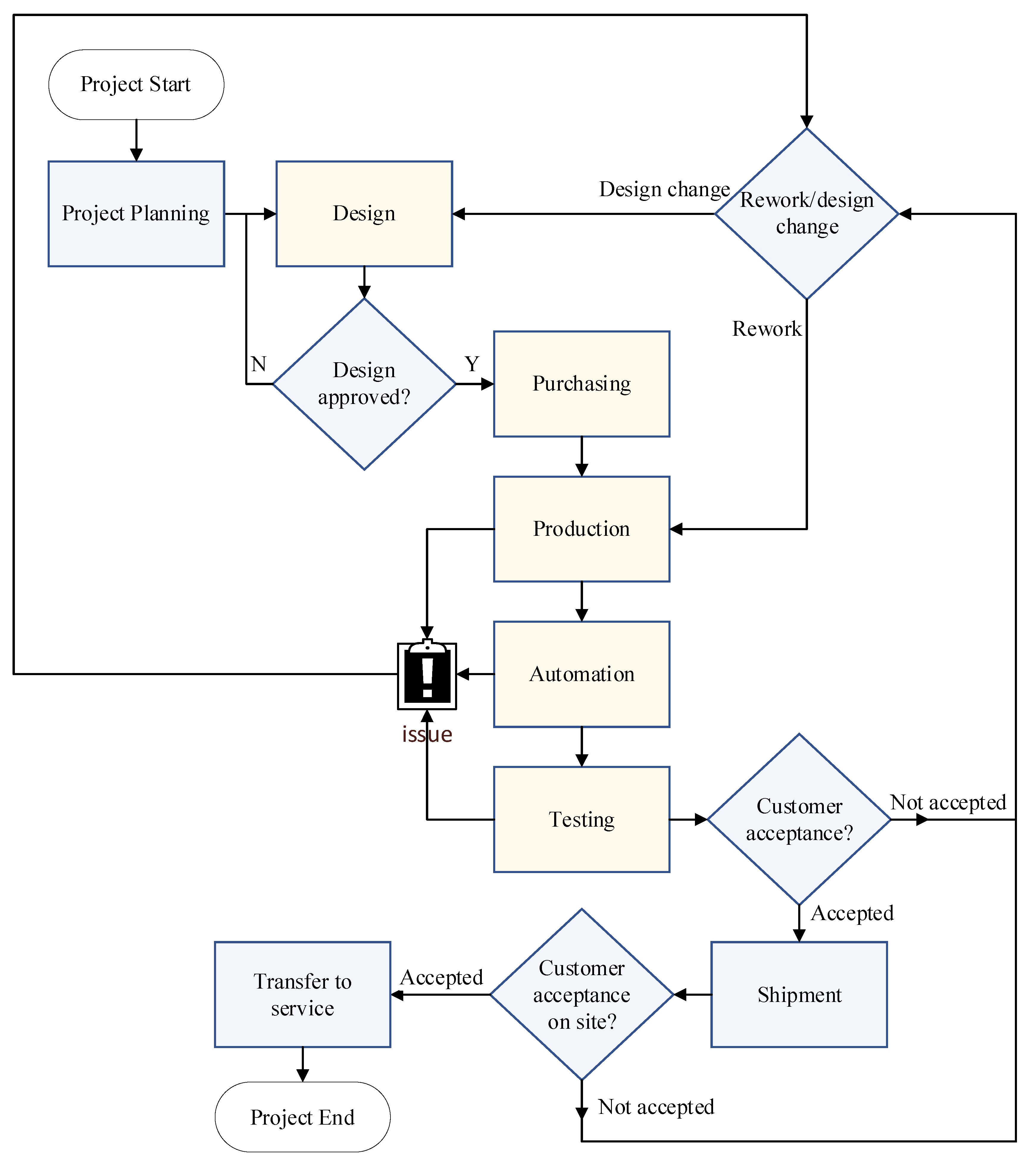
In this study, the ANN model was constructed using data collected from a company that designs and manufactures customized machines for the semiconductor industry. These machines are developed by considering the customer-specific product and process requirements to execute the process of customer products automatically. Machine development projects within this company mainly consist of four main phases: design, purchasing, production, automation, and testing, as shown in Figure 1. The project starts with the design phase, where the mechanical, electronic, and micro-optic components and subassemblies of the machine are designed according to the customers’ requirements. After the design is reviewed and approved by the customer, the machine’s bill of material is transferred to the purchasing team. Next, the process continues searching and selecting suppliers to purchase the necessary components and parts. As necessary components are delivered, according to the production plan, the assembly of the machine starts. The machine’s mechanic, electronic, and micro-optic components are assembled considering the drawings and an integration plan. Finally, equipment that works with the machine is integrated and tested, and the machine is prepared for automation.

Then, automation starts, and the process is developed to produce customer products automatically using the machine. The general software system, which has already been developed to control machines, is integrated into the machine, and the process steps are defined to control the necessary subassemblies and equipment integrated into the machine, in other words, to automate the production process of customer products. This phase is crucial since each customer has a specific product and process. In most cases, the customer production process is manual, and the product is manufactured for R&D purposes. During machine automation, effective communication is necessary to reconstruct the customer’s production process according to the machine’s capabilities. In some cases, the process is well-known for the company and has been previously developed for another customer. Therefore, the necessary effort is relatively less than needed to develop a new process. In conclusion, the necessary effort to develop a process and automate a machine can vary from machine to machine.

Effort drivers and categories were defined through brainstorming sessions with experts within the company and considering the studies mentioned in the literature review. First, eleven factors were selected, as listed below:

• Hardware complexity;
• Process complexity;
• Customer type;
• Customer product novelty;
• Customer process novelty;
• System configuration novelty;
• Machine function;
• Machine main system size;
• Machine housing size;
• Machine line type;
• Outsource usage for production.

Hardware complexity defines how complex the machine’s hardware design is. To evaluate this factor, two categories were used: low and high. Specific statements describing the attributes of the machine’s motion, vision, and data acquisition systems were defined for these two categories but are not explicitly presented here for security reasons. Process complexity defines the complexity level of the process of customer products and is categorized as low and high. Customer products can require more than one different process in a machine. Additionally, some processes can be more challenging due to the maturity level of the technology used and the company’s familiarity with the process. Therefore, some statements were identified for the low and high factor levels to prevent subjective assessment considering the above situations.

The factors regarding the customer type, product, and process novelty define how the company is familiar with this customer, product, and process. Customer type can be new or old. If the customer has already bought at least one machine before, the customer type is assessed as old. Two factors regarding customer product and process novelty have a three-point scale: no change, upgraded, and new. The level of “no change” defines the situation in which the customer has already previously purchased the same type of machine for the same customer product and process, so there is no significant change in the customer product or process. In the category of “upgraded”, the same type of machine is produced for upgraded customer products and processes. Although additional effort is needed due to the process changes for the automation phase, it is expected to be less than in the case of new products and processes. Since the company has experienced such machines and a process has been previously developed, the process can be developed for a new machine with minor adjustments. The last option, “new”, is when a customer is new, and the company has not previously experienced such products and processes with this customer. The factor of system configuration novelty is the novelty level of the sub-systems that comprise the entire system. This input is also on a three-point scale: no change, upgraded, and new.

The factor regarding machine function provides information about the machine’s primary function. It describes the process that the machine mainly executes and has five categories. The “machine main system size” factor includes six categories that define the complexity of the main sub-assembly that conducts the machine’s primary function, the number of subassemblies, and the components used. The housing size is the factor that defines the size of the exterior case of a machine that protects the internal mechanism. This factor is assessed in six categories: no housing, extra-small, small, medium, large, and extra-large. Most R&D-purpose machines are built without housing. An extra-small housing is usually chosen if a machine executes only one simple function including a few small subassemblies. A machine housing is considered as small when it is of below-average size. Medium-sized housing is used in machines that execute more than one function. If a machine is highly customized and performs more than one function, it includes many subassemblies. A larger size than average is needed for housing these kinds of machines. If a machine includes several big-sized subassemblies, the housing will be significantly larger than the average size.

The “machine line type” factor identifies the line type in terms of the production volume the machine will be used in, and has three categories: entry, standalone, and in-line. If the machine is produced for a low-volume production environment and produces a low-complexity product, the machine type is entry-level. In the standalone category, the machine can execute its primary function independently. If the machine is integrated within a line of several machines, it is described as an in-line machine. The last input is outsourcing usage for machine production and categorized as outsource used or in-house production.

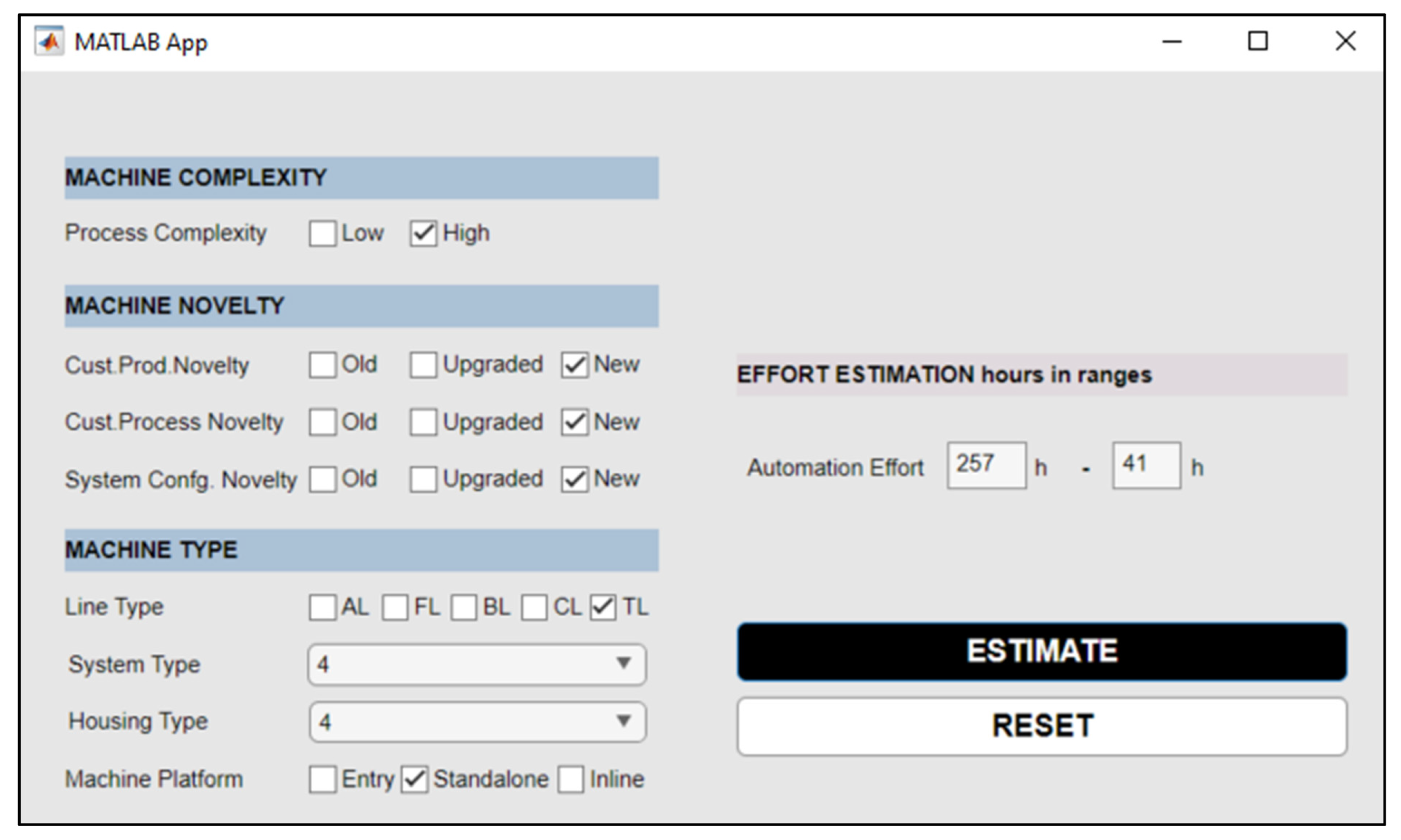
Automation effort is the output of the model. The automation effort value includes all of the efforts necessary to automate a machine. Person-hours were used to evaluate the automation effort value. This value was obtained from a database containing the company personnel’s time spent on projects. Then, revisions were made with the assistance of the company experts in the case of an error.

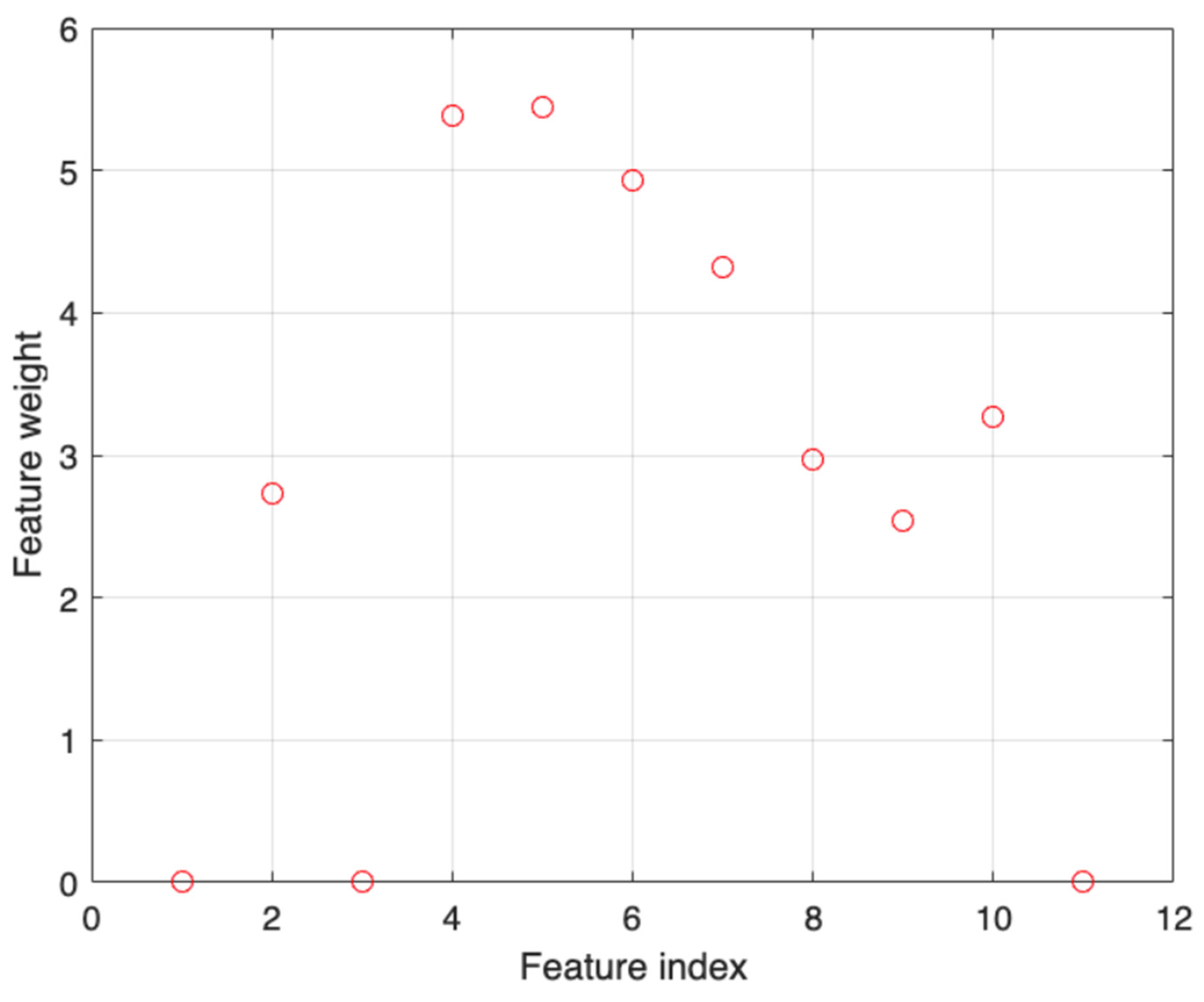
The data for the eleven effort drivers described above as well as the automation effort were collected from 101 completed projects. To maximize the prediction accuracy, neighborhood component analysis (NCA) was applied for feature selection. This nonparametric feature selection technique selects the best subsets of features by assigning weights to each feature. Based on the weights, the features with low weights can be removed from the input dataset. Instead of transforming the data into a different feature space as in principal component analysis (PCA), NCA assigns a weight to each feature. Similarly, individual features can be analyzed for relevance. While retaining features having significant weights, the rest can be eliminated. This technique was used by Goyal and Bhatia [27] to select features for a MLP-based model to estimate the software project effort. The eleven features listed above were used as predictors and automation efforts as a response. MATLAB was used for the implementation of the method. 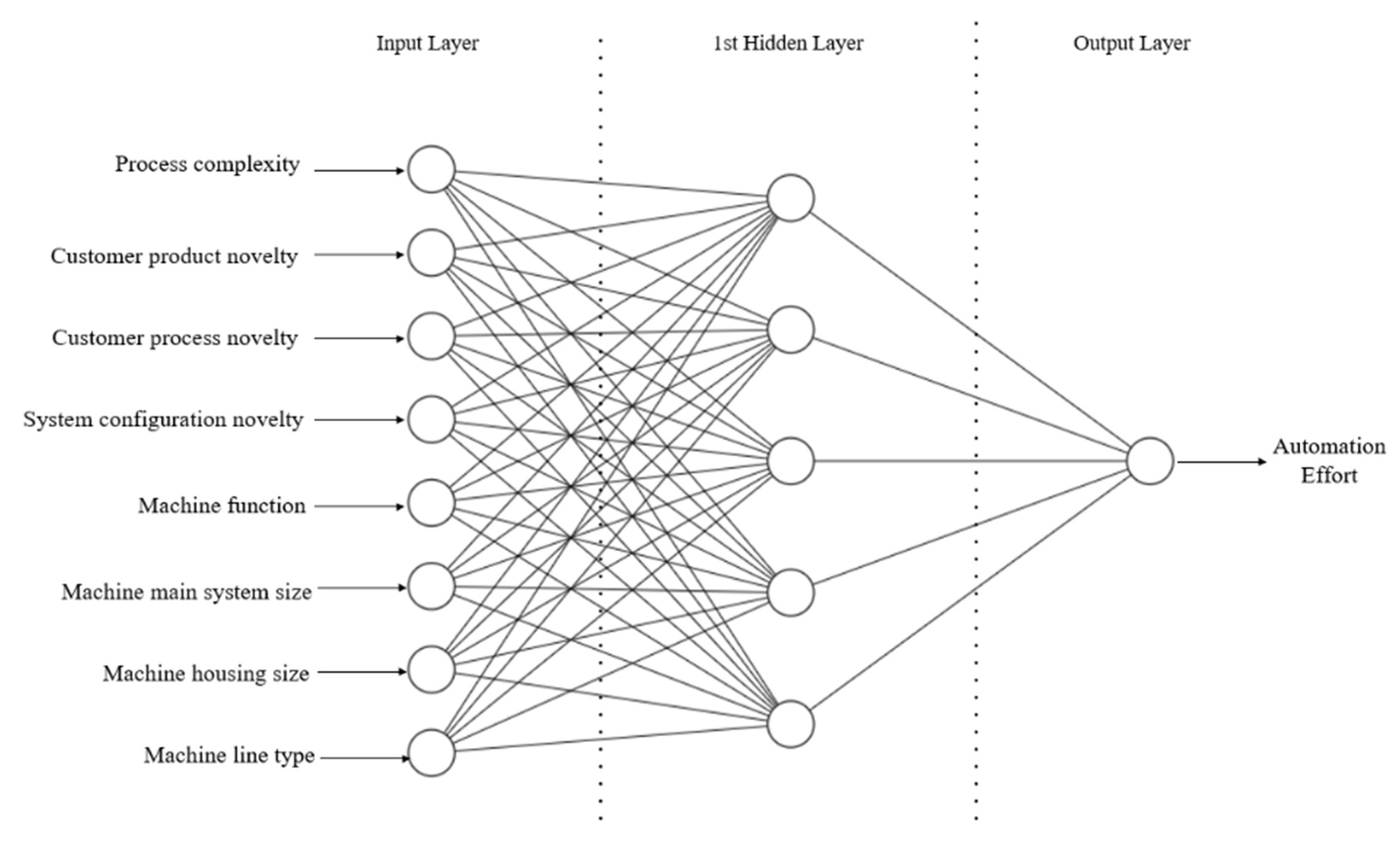As shown in Figure 2, features 1, 3, and 11 have zero weights. These features, hardware complexity, customer type, and outsource usage were eliminated from the dataset. The remaining features with significant weights were selected for the automation effort estimation. As a result, only eight out of 11 features were used in the ANN model. The inputs and output defined for the ANN model are shown in

Table 1. Selected features for the effort estimation.

No.	Variable Name	Level	Role
1	Process complexity	1: low, 2: high	Input
2	Customer product novelty	1: no change, 2: upgraded, 3: new	Input
3	Customer process novelty	1: no change, 2: upgraded, 3: new	Input
4	System configuration novelty	1: no change, 2: upgraded, 3: new	Input
5	Machine function	Five categories regarding types of functions based on a machine’s primary function	Input
6	Machine main system size	Six categories	Input
7	Machine housing size	1: No housing, 2: extra small, 3: small, 4: medium, 5: large, 6: extra large	Input
8	Machine line type	1: entry, 2: standalone, 3: in-line	Input
9	Automation effort	Required effort for the automation phase of a machine development project	Output

.

3.2. Hyperparameter Optimization of the Proposed ANN

One of the most widely used architectures in the field of effort estimation, FFNN, was used in this study. In the effort estimation area, gradient descent-based learning algorithms have been used to train an ANN [17,21,22]. However, there are some drawbacks. GD-based algorithms require the selection of hyperparameters such learning rate and momentum, which significantly affect the ANN performance. In addition, they require matrix calculations and have slow convergence due to gradient calculations. Levenberg–Marquardt is another learning algorithm to overcome the drawbacks of GD related to storage requirements. Since the LM algorithm does not require complex matrix calculations, learning rate, or momentum selection and has a higher convergence, it was chosen for this study. The LM method is also the most effective method for t FFNN structures.

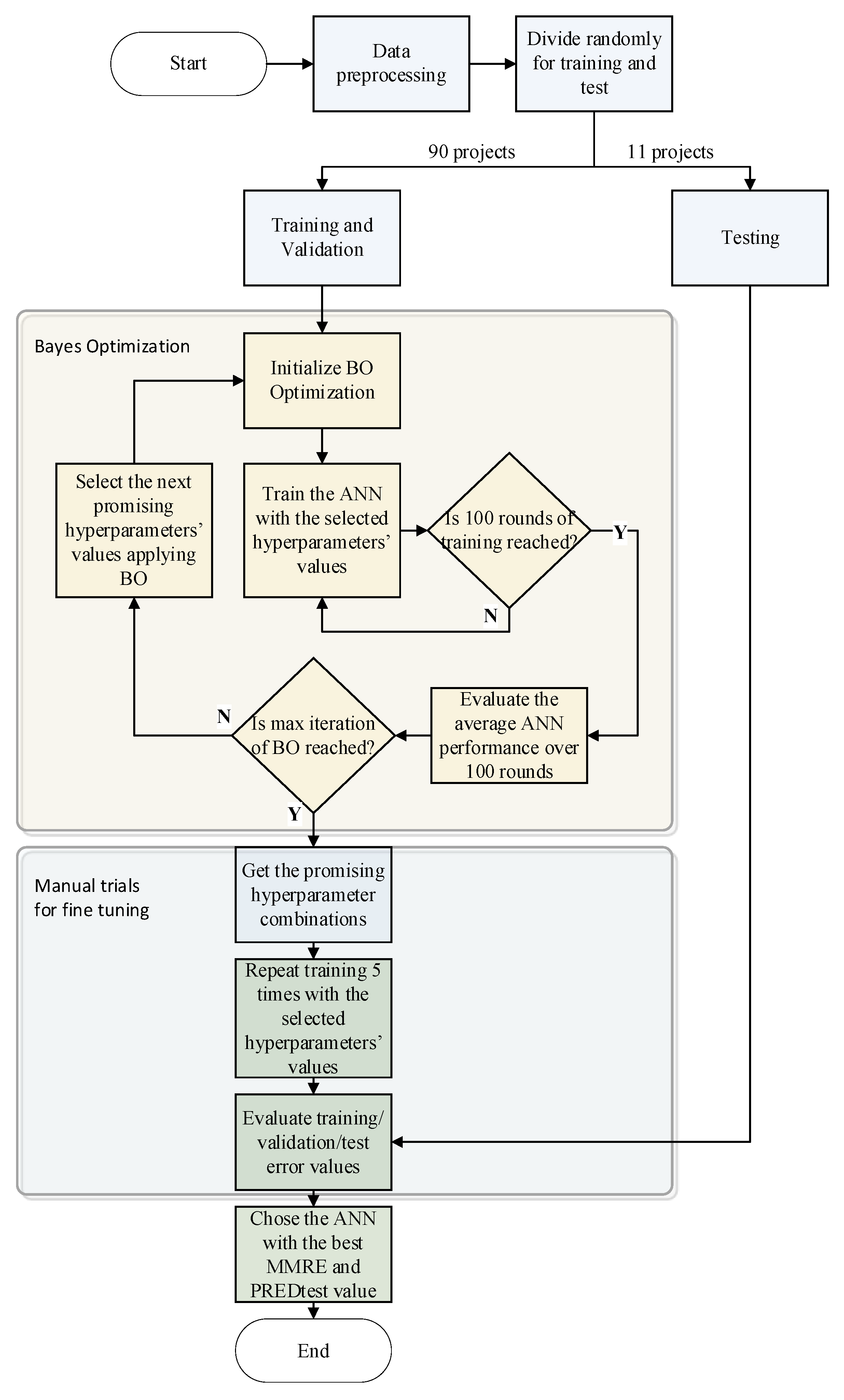
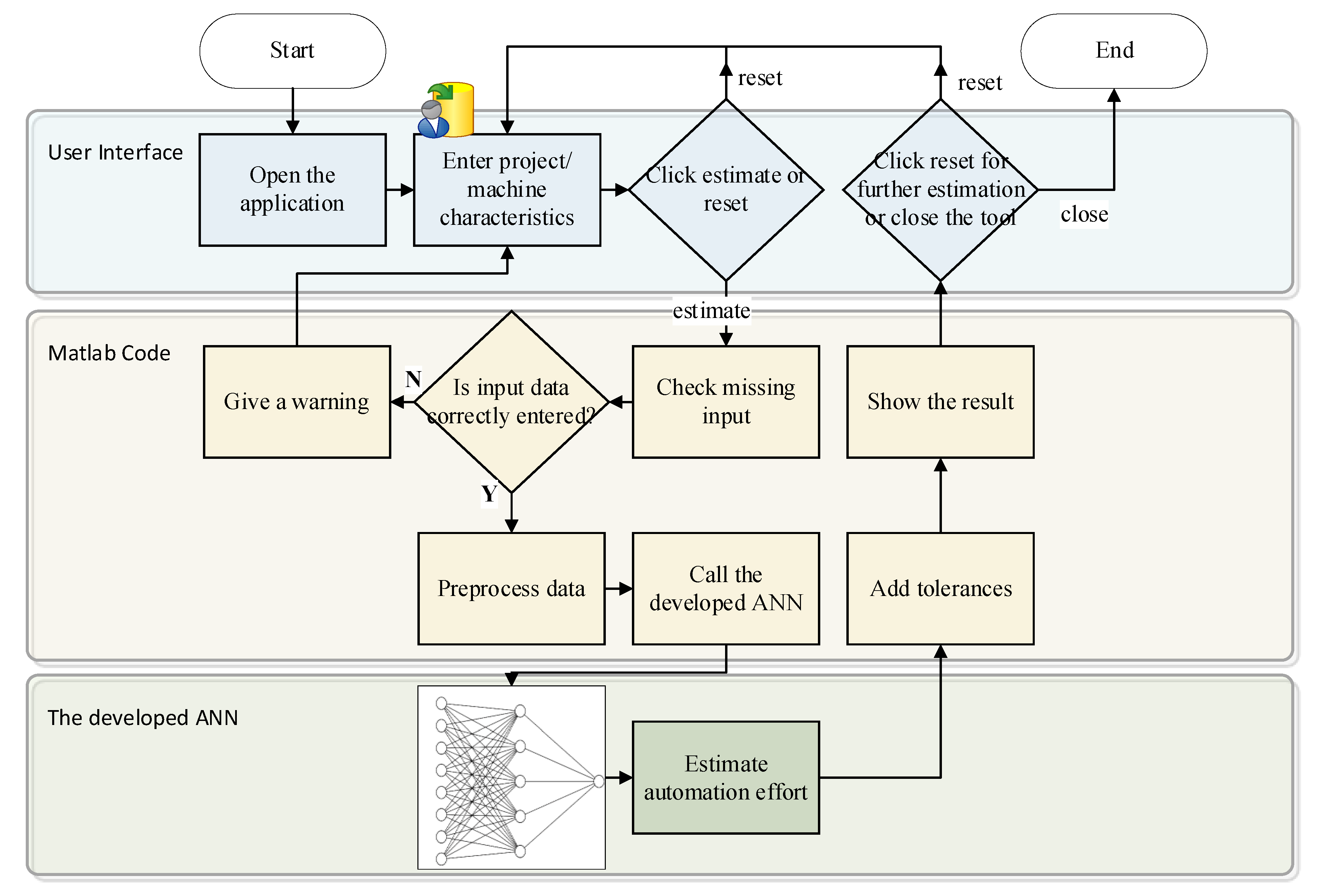
Most studies have reported that the FFNN structure outperforms other prediction models in software effort estimation. However, hyperparameter tuning is crucial to network performance. Any minor hyperparameter adjustment can significantly affect the prediction accuracy. For this purpose, one of the intelligent optimization methods, BO, was used to tune the hyperparameters. The procedure including BO for developing the network was programmed using MATLAB and is illustrated in Figure 3.

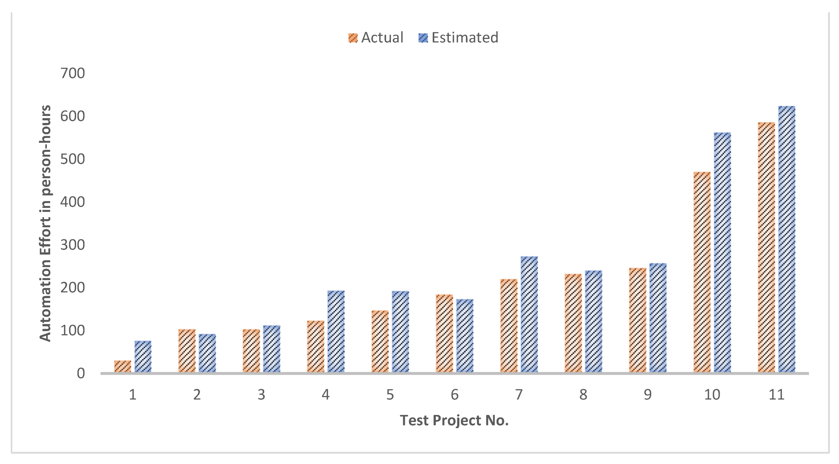
A min–max normalization was applied first to reduce the bias of the higher values. Normalization was applied to all of the input variables to make them all the same scale even though they were categorical. Additionally, a log transformation was applied to the output data to reduce skewness and make it more normal. After data preparation, the dataset containing 101 machine development projects was randomly divided into two parts: the training and test sets. The test data containing 11 projects were not shown to the ANN during training and was used only for testing purposes to understand the ANN performance on different datasets.

Next, model architecture development steps continued with the training data. The hyperparameters selected for optimization were the number of hidden neurons, activation functions in the hidden layers and the output layer, as shown in

Table 2. Hyperparameters to be optimized by BO.

Hyperparameters to be Optimized	Possible Values
The number of neurons at 1st HL	2–8
Activation function for 1st HL	tansig, logsig, purelin
Activation function for output layer	tansig, logsig, purelin

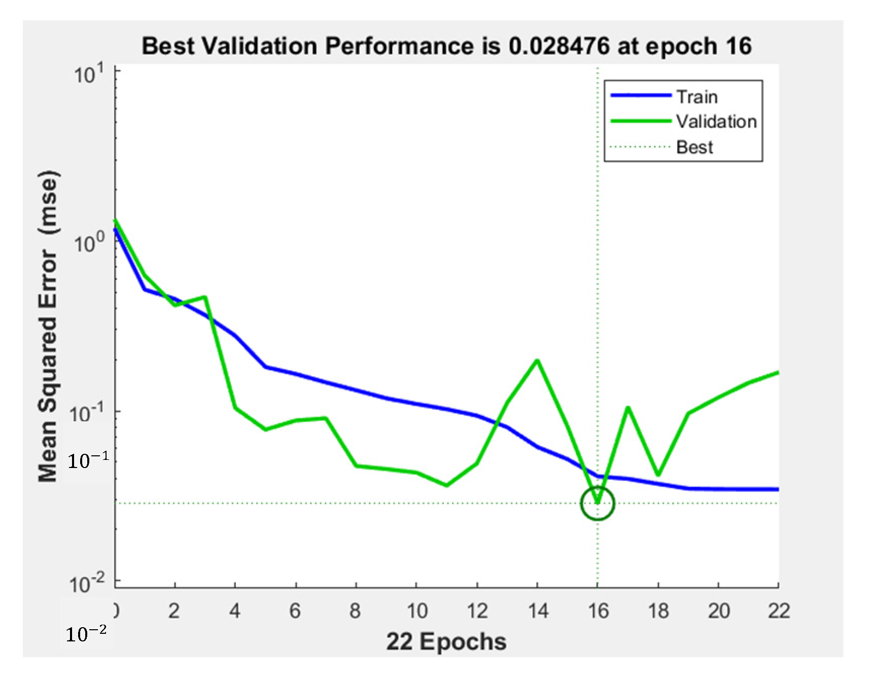
. In the effort estimation area, many studies have reached the best ANN structure with one hidden layer [8,9,19,22,29]. Thus, one hidden layer was used for this study. For the first hidden layer, the number of hidden neurons was set to between two and eight. The possible values for activation functions for the hidden and output layers were chosen as tansig, logsig, and purelin. The division ratio of the data that decides the percentage of projects used in the training and validation dataset was set as 90–10%. Validation performance is one of the crucial points to determine how well the training process is and when it is to be terminated. This training process is to be terminated when generalization stops to prevent overfitting, which means that the model obtained good results for training but not for validation. Therefore, the stopping criteria were chosen as the max validation failure, which means that the MSEval is higher than the MSEval-best in the last six times.

The BO procedure begins with the selection of the initial hyperparameter values. After setting the hyperparameters, the network is initialized with randomly selected initial weights and training and validation dataset combinations. Training with the selected hyperparameters was repeated 100 times, and the average validation error was calculated to determine the validation performance of the network on the different datasets. At each training round, samples for training and validation were randomly selected. This technique is known in the literature as repeated random subsampling validation (Monte Carlo cross-validation), which splits the dataset randomly into training and validation datasets and averages the results over the splits. Repeating the training and validation rounds 100 times helps a model to produce more repeatable results and increases the prediction robustness by repeating this process with different randomly chosen initial weights and a combination of training and validation datasets.

The evaluation method of mean squared errors (MSE) was chosen to assess the ANN performance. MSE can be calculated as per the following equation:

$${\mathrm{MSE}}_{\mathrm{val}}\left(\mathrm{j}\right)=\frac{{{\displaystyle \sum }}_{\mathrm{i}=1}^{\mathrm{n}}{\left({\mathrm{Actual} \mathrm{effort}}_{\mathrm{i}}-{\mathrm{Estimated} \mathrm{effort}}_{\mathrm{i}}\right)}^2}{\mathrm{n}}$$

(1)

$$\begin{gathered} \mathrm{n}: \mathrm{the} \mathrm{total} \mathrm{number} \mathrm{of} \mathrm{samples} \mathrm{in} \mathrm{validation} \mathrm{dataset} \\ \mathrm{j}:\mathrm{number} \mathrm{of} \mathrm{training} \mathrm{repeats}.{\forall }_{\mathrm{j}}\in \left\{1,2,\dots ,100\right\}. \end{gathered}$$

After 100 rounds of training, the average MSE value was calculated, as per the following equation:

$$\mathrm{avg}\left({\mathrm{MSE}}_{\mathrm{val}}\right)=\frac{{{\displaystyle \sum }}_{\mathrm{j}=1}^{100}{\mathrm{MSE}}_{\mathrm{val}}\left(\mathrm{j}\right)}{100}$$

(2)

The calculated average performance value was taken as an objective function of BO. Therefore, BO aims to find the best hyperparameter values that minimize this objective function.

After determining the average validation performance value over 100 rounds, BO builds a probability model of the unknown objective function using the observed objective function values. This prior probability model of the objective function is known as a surrogate model. Due to its simplicity and ease of optimization, the Gaussian process is most commonly used as a surrogate model. It provides a probabilistic representation of the objective function’s uncertainty at any given data point by building a multivariate Gaussian distribution from the historical data. The BO algorithm finds the next data point, the following promising hyperparameter value that performs best on the surrogate model. BO uses the acquisition function to find the next promising point on the surrogate model. The mostly used acquisition function is expected improvement. BO chooses the next data point that gives the max expected amount of improvement in the objective function. BO then obtains the objective function value by training ANN with the selected hyperparameters. Then, it updates GP prior distribution (surrogate model) with the new data to produce a posterior. This posterior will become the prior in the next step. This procedure is repeated until the stopping criteria of BO, 30 iterations.

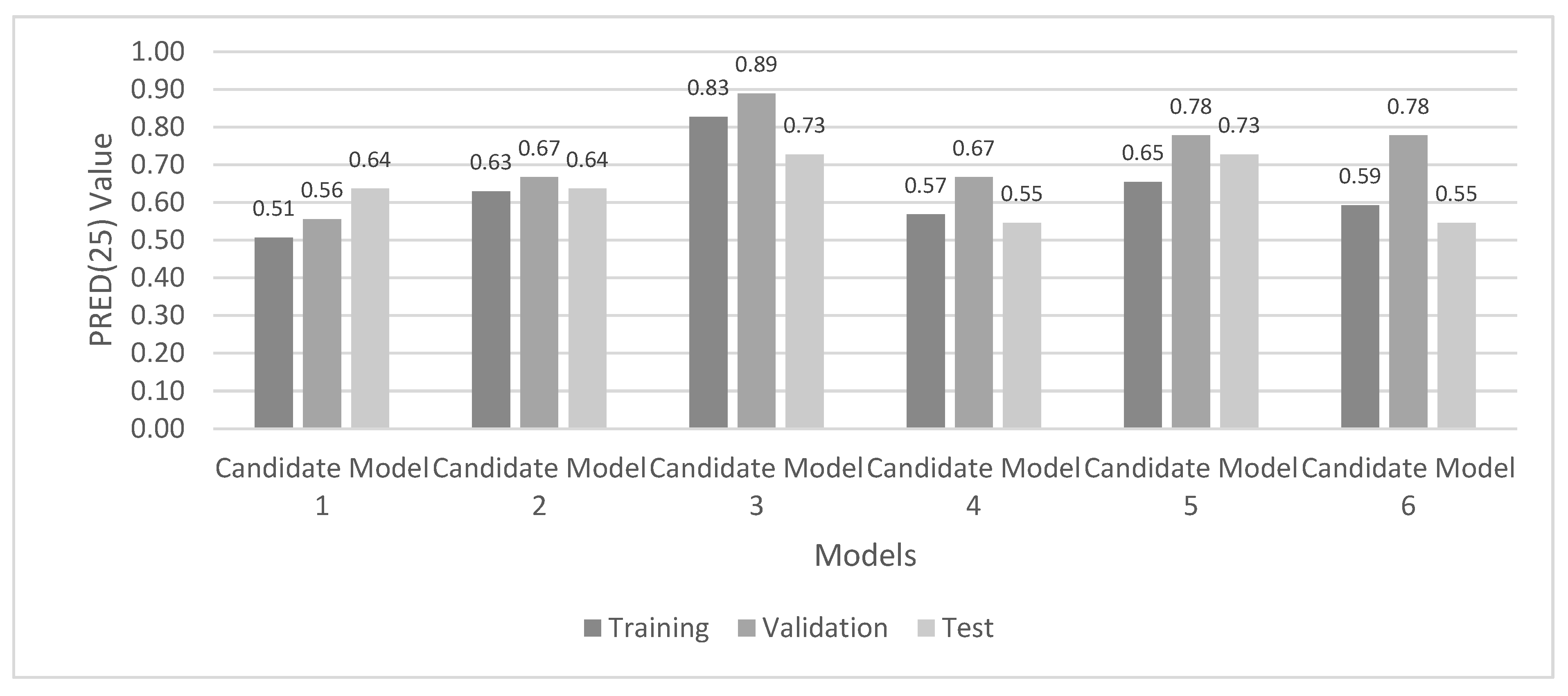
According to the results of the BO, the optimal hyperparameter values and a number of hyperparameter combinations that produce promising results were selected. For each combination, training was repeated five times. For each round, the ANN test performance was calculated over a test dataset containing 11 projects.

The mean magnitude of relative errors (MMRE) and prediction accuracy (PRED) were used to evaluate the ANN performance. Several methods exist to evaluate the performance of ANNs and determine how well they match the desired output. In the effort estimation area, MMRE and $\mathrm{PRED}\left(\mathrm{x}\right)$ are commonly used methods for calculating model performance. MMRE is the mean of the magnitude of relative errors (MRE), which is calculated for each observation $i$, expressed by the following equation:

$${\mathrm{MRE}}_{\mathrm{i}}=\left(\frac{\left|{\mathrm{Actual} \mathrm{Effort}}_{\mathrm{i}}-{\mathrm{Estimated} \mathrm{Effort}}_{\mathrm{i}}\right| }{{\mathrm{Actual} \mathrm{Effort}}_{\mathrm{i}}}\right)$$

(3)

MMRE is achieved by aggregating the MRE over multiple observations $i$ as in the following equation:

$$\mathrm{MMRE}=100\times \left(\frac{1}{\mathrm{N}}\right){\displaystyle \sum }_{\mathrm{i}=1}^{\mathrm{N}}{\mathrm{MRE}}_{\mathrm{i}}$$

(4)

By using MRE values, $\mathrm{PRED}\left(\mathrm{x}\right)$ can be calculated as the average of the MREs (or MERs) that are less than or equal to $\mathrm{x}$ [7], as shown in the equation below:

$$\mathrm{PRED}\left(\mathrm{x}\right)=\frac{1}{\mathrm{N}}{\displaystyle \sum }_{\mathrm{i}=1}^{\mathrm{N}}\left\{\begin{array}{c}1 \mathrm{if} {\mathrm{MRE}}_{\mathrm{i}}\le \mathrm{x}\\ 0 \mathrm{otherwise}\end{array}\right.$$

(5)

Model accuracy is directly proportional to $\mathrm{PRED}\left(\mathrm{x}\right)$ and inversely proportional to MMER or MMRE [7]. $\mathrm{PRED}\left(\mathrm{x}\right)$ represents the percentage of project effort estimates that are within $\%\mathrm{x}$ of the actual [8]. In many studies, the value of x is taken as 25 [11,22,31]. A model with the prediction accuracy of MMRE $\le 25\%$ and PRED(25)$\ge$75% are considered sufficient for software effort prediction [9].

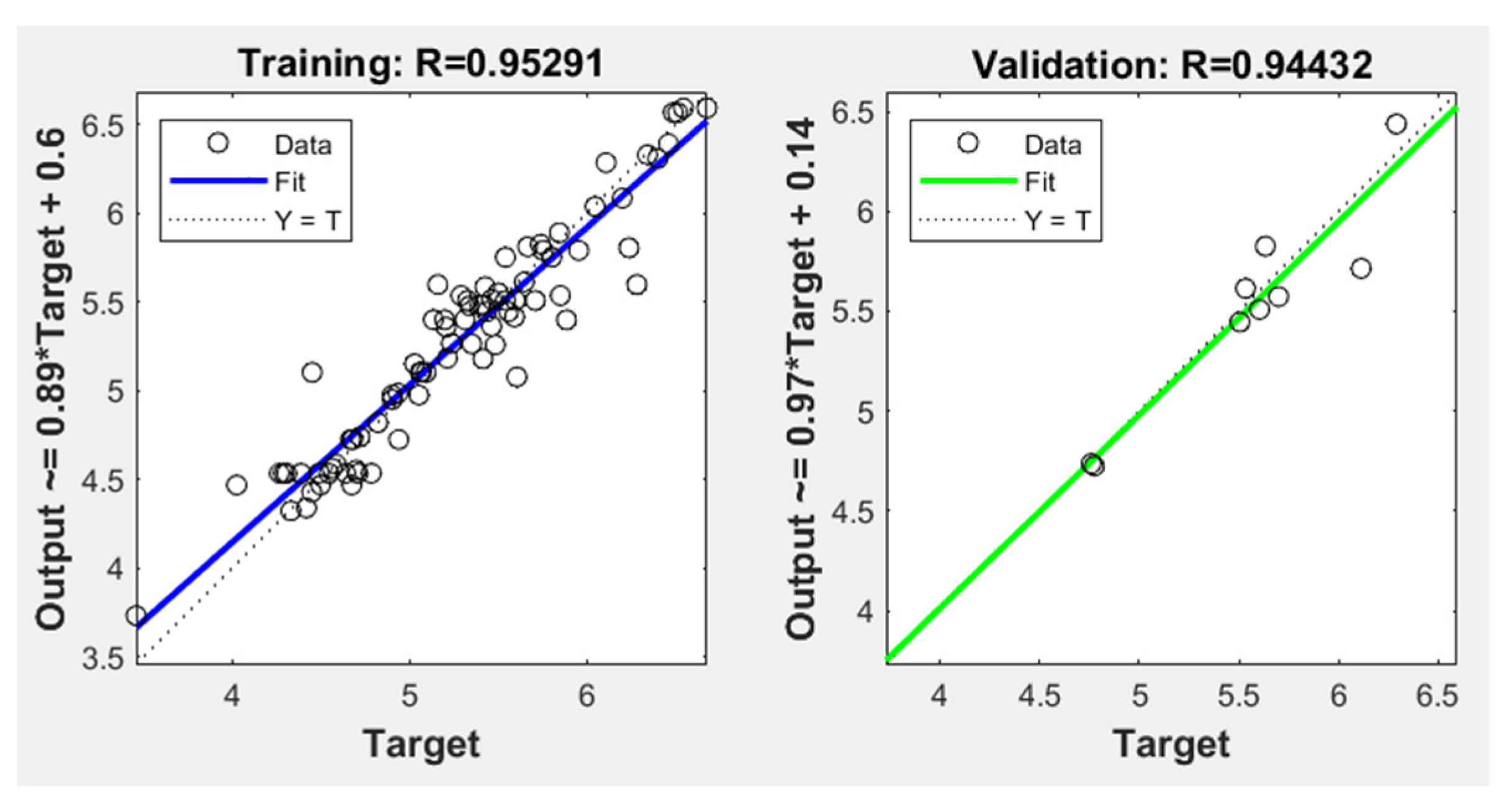
Before calculating MMRE and PRED(25) for each training experiment, the output values were transformed to original values from the logarithmic. After calculating the ANN test performance over the test data for each training experiment, the network with the best MMRE and PRED(25) values was selected.

4. Results and Discussion

4.1. The Architecture and Performance of the Proposed ANN

The methodology described in the preceding section was applied to a dataset comprising 101 completed machine development projects. As above-mentioned, 90 were used for training, and the rest for testing. To determine the best hyperparameter values, BO was applied. BO provided an idea of which combination of hyperparameter values produced the best mean validation error value of the ANN over 100 rounds of training and validation. The BO results showed that the optimal value of the objective function was obtained at the sixth iteration with the best objective function value of 0.19718.

The optimal structure consisted of one hidden layer with four neurons and logsig and purelin activation functions for the hidden and output layers. The second-best result was produced in the fifth iteration using the same activation functions but with six neurons. In addition, the error values for structures with three and five neurons using the same activation functions as the optimal structure were close to the optimal value. Since the objective function of the best structure is 0.19756 and taking into account the conditions above-mentioned, structures with error value less than 0.20500 were selected for further evaluation. The training was repeated five times for each of the hyperparameter combinations shown in

Table 3. The selected hyperparameter combinations for further evaluation.

Iteration Number	Observed Objective	The Number of Hidden Neurons	Activation Function of the Hidden Layer	Activation Function of the Output Layer
5	0.19756	6	logsig	purelin
6	0.19718	4	logsig	purelin
7	0.20445	5	logsig	purelin
8	0.19865	3	logsig	purelin
9	0.19934	4	tansig	purelin
10	0.20332	6	tansig	purelin

.

The initial weights and projects for training and validation were randomly chosen in each round by considering the 90–10% division ratio. The ANN was tested with 11 test projects for each round. By considering the MMRE and PRED(25) values, the ANN model that provided the best performance was selected. The structure that yielded 70% PRED(25) and 30% MMRE for all of the training, validation, and test datasets was selected. The architecture of the ANN that obtained the best performance is shown in Figure 4.

The training was terminated at epoch 16 when the validation MSE error was greater than the best validation MSE for the last six trials, as shown in Figure 5.

The performance values of the optimal architecture are given in

Table 4. Performance values of the best ANN architecture.

	MSElog	R-Value	MMRE	PRED(25)
Training	0.04	0.95	0.15	0.83
Validation	0.03	0.94	0.13	0.89
Test	0.11	0.94	0.30	0.73

and the correlation (R) values are shown in Figure 6. For the values, MMRE and PRED, re-transforming was applied to the results from the logarithmic values to the original.

Estimated values of the proposed ANN model and the actual values of the automation efforts for the test results are shown in Figure 7. The logarithmic output values were re-transformed back to their original form to compare the estimated values to the actual values.

Studies that have used artificial neural networks in the field of effort estimation have mainly focused on software projects. In this area, models with a MMRE less than 25% and PRED(25) higher than 75% are considered as accurate [9].

Table 5. Summary table on the prediction accuracies from studies in the effort estimation area.

Year	Author(s)	Ref.	Method	Prediction Accuracy
2002	Heiat	[13]	RBFNN	MAPE: 31.96%
2008	Tronto et al.	[8]	MLP	MMRE: 41.53%
2008	Park and Baek	[18]	ANN	MRE: 59.40%
2010	Reddy, Sudha, Rama, Ramesh	[45]	RBFNN, GRNN	MMRE: 17.29%, 34.61%
2010	Kalichanin-Balich and Lopez-Martin	[46]	FFNN	MMER: 22%
2011	Lopez-Martin et al.	[10]	GRNN	MMER: 26%
2011	Attarzadeh and Ow	[19]	MLP	MMRE: 45%, PRED(25): 43.30%
2012	Attarzadeh et al.	[22]	FFNN	MMRE: 46%, PRED(25): 45.50%
2013	Nassif et al.	[7]	MLP	MMER: 40%, PRED(25): 45.70%
2013	Pai, McFall, Subramanian	[38]	MLP	MMRE: 59.30%
2016	Rijwani and Jain	[21]	FFNN	MMRE: 14.40%
2018	Pospieszny et al.	[9]	MLP	MMRE: 21%, PRED(25): 64.65%, MMER: 45%
2020	Goyal and Bhatia	[29]	FFNN	MMRE: 25.80%, R-value: 90%
2020	Pandey et al.	[31]	MLP	MMRE: 24%, PRED(25): 42%
2021	Rankovic et al.	[20]	MFFN with the Taguchi method	MMRE: 16.10%, PRED(25): 50%
2021	Carvalho, Fagundes, Santos	[5]	MLP, Extreme Learning Machine	MMRE: 42%, 18%
2022	Sharma and Vijayvargiya	[47]	Wavelet ANN, Genetic Elephant Herding Optimization-based Neuro-Fuzzy Network	MMRE: 22.08%, 16.70%

summarizes the results from various studies that have used neural networks to estimate the project effort. According to Table 5, the MMRE values ranged from 14% to 59% and the PRED values ranged from 42% to 65%.

Among the trials, some candidate models with MMRE values of at most 45% and PRED values of at least 50% are listed in

Table 6. List of candidate models and the best ANN.

The Number of Hidden Neurons	Activation Function	Experiment No. (Appendix A)	Candidate Model No.	MMRE			PRED(0.25)
				Tra	Val	Test	Tra	Val	Test
3	logsig	5	1	0.31	0.28	0.40	0.51	0.56	0.64
4	logsig	5	2	0.27	0.22	0.40	0.63	0.67	0.64
5	logsig	4	3	0.15	0.13	0.30	0.83	0.89	0.73
6	logsig	3	4	0.28	0.33	0.43	0.57	0.67	0.55
4	tansig	3	5	0.24	0.20	0.41	0.65	0.78	0.73
6	tansig	1	6	0.27	0.26	0.42	0.59	0.78	0.55

. For the output layer, a linear activation function, purelin was selected. The PRED(25) results are presented in Figure 8 as well as the best model (candidate model 3).

In order to assess the effectiveness of ANN models for customized machine development projects, the proposed ANN model was compared with multiple linear regression (MLR). The MLR was applied with the same training data used to train the ANN. Data from eleven test projects were used to evaluate the performance of the regression model.

Table 7. Comparison of the performance of the proposed ANN and MLR.

	MMRE		PRED(25)		MAE		RMSE
	MLR	Proposed ANN	MLR	Proposed ANN	MLR	Proposed ANN	MLR	Proposed ANN
Training	0.54	0.15	0.32	0.83	94.54	32.77	128.09	52.79
Validation	0.27	0.13	0.78	0.89	57.17	44.25	67.17	62.85
Test	0.92	0.30	0.27	0.73	96.82	35.89	115.33	45.03

provides a comparison between the results generated by MLR and the proposed ANN. Comparing the proposed ANN with the MLR, it can be seen that the performance of the proposed ANN was much better than the MLR.

4.2. The ANN-Based Estimation Tool for Automation Effort of Machine Development Project

An automation effort estimation tool was developed using MATLAB 2022a App Designer. The tool evaluates the total effort needed to develop a process for a machine to produce customer products automatically. The process flow of the tool is given in Figure 9.

A real-life example of how the effort estimation tool works is provided as follows. This example is also the second test project presented in the previous section.

Table 8. Selected values of the example to demonstrate how the ANN tool works.

No.	Input Name	Selected Value	No.	Input Name	Selected Value
1	Process complexity	High	5	Machine function	Test machine
2	Customer product novelty	New	6	Machine main system size	Medium
3	Customer process novelty	New	7	Machine housing size	Medium
4	System configuration novelty	New	8	Machine line type	Standalone

shows the selected values of the project characteristics for the example. As depicted in Figure 9, the user enters the project characteristics. The first characteristic of the machine is its process complexity. As indicated, the possible values for machine function type, main system size, and housing size are not explicitly listed due to the company’s information security policies. As a result, limited information is provided here. For this example, a new customer requests a testing machine that will run complex testing procedures on the customer’s specific product. Additionally, the customer requires that the machine meets a certain cycle time for this testing process. Therefore, a high level of process complexity was selected.

The second and third inputs were related to the novelty of the customer’s product and process. If the company has no prior experience with this customer, the product, or process, the second and third input values are selected as new. The fourth input specifies the novelty degree of the system configuration. Since the company has never previously developed this process for this customer, a new configuration is chosen. The core system, which performs the machine’s primary function, and housing size are selected as the medium. Finally, the machine line type is determined to be standalone since the machine can execute the test function without assistance from another machine and can conduct the necessary tests by itself.

Figure 10 depicts the user interface for entering these characteristics. After entering the values, the user clicks the “estimate” button to see the estimations. Suppose that each input characteristic is entered, and only one option is chosen for each of them. In that case, the system works and obtains the estimated automation effort value from the output of the developed ANN. The ANN-based estimation tool provides project effort estimates with tolerances. This tolerance value was determined using the MRE values of the data points in the training, validation, and test data. The average MRE estimated across all datasets was calculated as 0.16. To illustrate, the program predicts that 257 person-hours will be required to automate a machine development project using the above-listed project parameters. This was shown with a tolerance value of $257\times 0.16\cong 41$ person-hours at the user interface.

In the company’s current process, effort estimations for the automation phase of a project are performed during project kick-off. After the order confirmation is received from the customer and the project is approved to start, the technical sales team transfers the project with the project charter to the project manager. Then, a project kick-off meeting is organized with the attendance of the necessary function line managers. Next, the planning phase starts, and the project manager makes effort estimations for project phases with the support of function line managers. It can be challenging for project managers to provide a reasonable estimate of the amount of effort required if they have no experience with a project similar to the one that they are attempting to predict.

Especially at the early stages of a project, estimating the amount of work required to automate a machine can be challenging due to the high level of uncertainty. The process to be developed is unique to the product and the process of the customer. The customer needs an automated machine for a process they currently perform manually. In most cases, the production flow of customer products needs to be redesigned. In some cases, the process is well-known and has been experienced with the same or a different customer. In such situations, the effort required is less than that needed to develop a new process. In conclusion, estimating the required effort is challenging because it varies from machine to machine. The proposed ANN tool can support project managers in estimating the automation efforts when faced with machine development projects of different specifications, even if they have limited experience with similar machines.

5. Conclusions

This paper presented a BO-based ANN model that was developed to estimate the automation effort for machine development projects. To the extent of our knowledge, no study has been conducted to estimate the automation effort for customized machine development. Because the uncertainty is high, effort estimation is still difficult, especially for projects that produce a customer-specific machine that automates the customer’s production process. A high level of uncertainty and lack of experience cause poor estimations of effort in the early phases of a project. Therefore, this study proposed a model to estimate the required effort to automate a machine.

One of the main reasons for project failure is poor effort estimation, and nowadays, researchers prefer objective approaches over expert-based approaches. Therefore, in this study, an ANN model was developed to overcome the shortcomings related to effort estimation. Data containing project characteristics and automation effort were collected from 101 real-life projects.

In this study, BO was used to optimize the hyperparameters. The performance of the best ANN architecture showed promising results. Effort estimation results are usually evaluated based on the PRED(25). According to some studies in the effort estimation area, the PRED(25) value ranges from 42% to 65%. In this study, the PRED(25) value was calculated as 83% for training, 89% for validation, and 73% for test projects. The accuracy of the developed model was quite good compared with other studies in project effort estimation. If required, the accuracy of the model can be improved by increasing the number of test projects. The proposed ANN model was applied to the real-life project effort estimation problem of a company in the customized machine development area. Moreover, a user-friendly ANN-based estimation tool was developed for effort estimators and project managers.

References

1. Hameed, S.; Elsheikh, Y.; Azzeh, M. An optimized case-based software project effort estimation using genetic algorithm. Inf. Softw. Technol. 2023, 153, 107088. [Google Scholar] [CrossRef]
2. Usman, M.; Britto, R.; Damm, L.O.; Börstler, J. Effort estimation in large-scale software development: An industrial case study. Inf. Softw. Technol. 2018, 99, 21–40. [Google Scholar] [CrossRef]
3. Monika; Sangwan, O.P. Software effort estimation using machine learning techniques. In Proceedings of the 7th International Conference on Cloud Computing, Data Science & Engineering–Confluence, Noida, India, 12–13 January 2017. [Google Scholar] [CrossRef]
4. Jørgensen, M.; Sjøberg, D.I.K. The impact of customer expectation on software development effort estimates. Int. J. Proj. Manag. 2004, 22, 317–325. [Google Scholar] [CrossRef]
5. Carvalho, H.D.P.; Fagundes, R.; Santos, W. Extreme learning machine applied to software development effort estimation. IEEE Access 2021, 9, 92676–92687. [Google Scholar] [CrossRef]
6. Prater, J.; Kirytopoulos, K.; Ma, T. Optimism bias within the project management context. Int. J. Manag. Proj. Bus. 2017, 10, 370–385. [Google Scholar] [CrossRef]
7. Nassif, A.B.; Ho, D.; Capretz, L.F. Towards an early software estimation using log-linear regression and a multilayer perceptron model. J. Syst. Softw. 2013, 86, 144–160. [Google Scholar] [CrossRef]
8. Tronto, I.F.B.; Silva, J.D.S.; Sant’Anna, N. An investigation of artificial neural networks based prediction systems in software project management. J. Syst. Softw. 2008, 81, 356–367. [Google Scholar] [CrossRef]
9. Pospieszny, P.; Czarnacka-Chrobot, B.; Kobylinski, A. An effective approach for software project effort and duration estimation with machine learning algorithms. J. Syst. Softw. 2018, 137, 184–196. [Google Scholar] [CrossRef]
10. López-Martín, C.; Chavoya, A.; Meda-Campaña, M.E. Software development effort estimation in academic environments applying a general regression neural network involving size and people factors. In Proceedings of the Pattern Recognition, 3rd Mexican Conference, MCPR, Cancun, Mexico, 29 June–2 July 2011; pp. 269–277. [Google Scholar] [CrossRef] [Green Version]
11. Koch, S.; Mitlöhrer, J. Software project effort estimation with voting rules. Decis. Support Syst. 2009, 46, 895–901. [Google Scholar] [CrossRef]
12. Arora, S.; Mishra, N. Software cost estimation using artificial neural network. Adv. Intell. Syst. Comput. 2018, 584, 51–58. [Google Scholar] [CrossRef]
13. Heiat, A. Comparison of artificial neural network and regression models for estimating software development effort. Inf. Softw. Technol. 2002, 44, 911–922. [Google Scholar] [CrossRef]
14. Bashir, H.A.; Thomson, V. Estimating design effort for GE hydro projects. Comput. Ind. Eng. 2004, 45, 195–204. [Google Scholar] [CrossRef]
15. Yurt, Z.O.; Iyigun, C.; Bakal, P. Engineering effort estimation for product development projects. In Proceedings of the IEEE International Conference on Industrial Engineering and Engineering Management, Macao, China, 15–18 December 2019. [Google Scholar] [CrossRef]
16. Ali, A.; Gravino, C.A. systematic literature review of software effort prediction using machine learning methods. J. Softw. Evol. Process 2019, 31, 1–25. [Google Scholar] [CrossRef]
17. Dave, V.S.; Dutta, D.M.K. Application of Feed-Forward Neural Network in Estimation of Software Effort. IJCA Int. Symp. Devices MEMS Intell. Syst. Commun. 2011, 5, 5–9. [Google Scholar]
18. Park, H.; Baek, S. An empirical validation of a neural network model for software effort estimation. Expert Syst. Appl. 2008, 35, 929–937. [Google Scholar] [CrossRef]
19. Attarzadeh, I.; Ow, S.H. Software development cost and time forecasting using a high performance artificial neural network model. In Proceedings of the Intelligent Computing and Information Science, International Conference, Part I, Chongqing, China, 8–9 January 2011; pp. 18–26. [Google Scholar] [CrossRef]
20. Rankovic, N.; Rankovic, D.; Ivanovic, M.; Lazic, L. Improved effort and cost estimation model using artificial neural networks and taguchi method with different activation functions. Entropy 2021, 23, 854. [Google Scholar] [CrossRef]
21. Rijwani, P.; Jain, S. Enhanced software effort estimation using multi layered feed forward artificial neural network technique. Procedia Comput. Sci. 2016, 89, 307–312. [Google Scholar] [CrossRef] [Green Version]
22. Attarzadeh, I.; Mehranzadeh, A.; Barati, A. Proposing an enhanced artificial neural network prediction model to improve the accuracy in software effort estimation. In Proceedings of the International Conference on Computational Intelligence, Communication Systems and Networks, Phuket, Thailand, 24–26 July 2012; pp. 167–172. [Google Scholar] [CrossRef]
23. Predescu, E.F.; Stefan, A.; Zaharia, A.V. Software effort estimation using multilayer perceptron and long short term memory. Inform. Econ. 2019, 23, 76–87. [Google Scholar] [CrossRef]
24. Jaifer, R.; Beauregard, Y.; Bhuiyan, N. New Framework for effort and time drivers in aerospace product development projects. Eng. Manag. J. 2021, 33, 76–95. [Google Scholar] [CrossRef]
25. Arundacahawat, P.; Roy, R.; Al-Ashaab, A. An analogy-based estimation framework for design rework efforts. J. Intell. Manuf. 2013, 24, 625–639. [Google Scholar] [CrossRef]
26. Pollmanns, J.; Hohnen, T.; Feldhusen, J. An information model of the design process for the estimation of product development effort. In Proceedings of the 23rd CIRP Design Conference, Smart Product Engineering, Bochum, Germany, 11–13 March 2013; pp. 885–894. [Google Scholar] [CrossRef]
27. Salam, A.; Bhuiyan, N.F.; Gouw, G.J.; Raza, S.A. Estimating design effort in product development: A case study at Pratt & Whitney Canada. In Proceedings of the International Conference on Industrial Engineering and Engineering Management, Singapore, 2–4 December 2007. [Google Scholar] [CrossRef]
28. Singh, A.J.; Kumar, M. Comparative analysis on prediction of software effort estimation using machine learning techniques. In Proceedings of the 1st International Conference on Intelligent Communication and Computational Research (ICICCR-2020), Delhi, India, 20–22 February 2020. [Google Scholar] [CrossRef]
29. Goyal, S.; Bhatia, P.K. Feature selection technique for effective software effort estimation using multi-layer perceptrons. Emerging trends in information technology. In ICETIT 2019, Emerging Trends in Information Technology; Springer: Berlin/Heidelberg, Germany, 2020; pp. 183–194. [Google Scholar] [CrossRef]
30. Azzeh, M.; Nassif, A.B. A hybrid model for estimating software project effort from Use Case Points. Appl. Soft Comput. J. 2016, 49, 981–989. [Google Scholar] [CrossRef]
31. Pandey, M.; Litoriya, R.; Pandey, P. Validation of existing software effort estimation techniques in context with mobile software applications. Wirel. Pers. Commun. 2020, 110, 1659–1677. [Google Scholar] [CrossRef]
32. Holzmann, V.; Zitter, D.; Peshkess, S. The expectations of project managers from artificial intelligence: A Delphi Study. Proj. Manag. J. 2022, 53, 438–455. [Google Scholar] [CrossRef]
33. Haykin, S.S. Neural Networks and Learning Machines, 3rd ed.; Prentice Hall/Pearson: London, UK, 2008. [Google Scholar]
34. Kumar, P.S.; Behera, H.S.; Kumari, A.K.; Nayak, J.; Naik, B. Advancement from neural networks to deep learning in software effort estimation: Perspective of two decades. Comput. Sci. Rev. 2020, 38, 100288. [Google Scholar] [CrossRef]
35. Rao, P.S.; Kumar, R.K. Software effort estimation through a generalized regression neural network. In Proceedings of the Emerging ICT for Bridging the Future, Advances in Intelligent Systems and Computing, the 49th Annual Convention of the Computer Society of India, Hyderabad, India, 11–15 December 2015; Volume 337, pp. 19–30. [Google Scholar] [CrossRef]
36. Makarova, A.; Shen, H.; Perrone, V.; Klein, A.; Faddoul, J.B.; Krause, A.; Seeger, M.; Archambeau, C. Overfitting in Bayesian optimization: An empirical study and early-stopping solution. In Proceedings of the 2nd Workshop on Neural Architecture Search at ICLR, Online, 7 May 2021. [Google Scholar]
37. Jun, E.S.; Lee, J.K. Quasi-optimal case-selective neural network model for software effort estimation. Expert Syst. Appl. 2001, 21, 1–14. [Google Scholar]
38. Pai, D.R.; McFall, K.S.; Subramanian, G.H. Software effort estimation using a neural network ensemble. J. Comput. Inf. Syst. 2013, 53, 49–58. [Google Scholar] [CrossRef]
39. Hutter, F.; Kotthoff, J.; Vanschoren, J. Automated Machine Learning: Methods, Systems, Challenges; Springer: Berlin/Heidelberg, Germany, 2019; Chapter 1. [Google Scholar] [CrossRef]
40. Zheng, A. Evaluating Machine Learning Models: A Beginner’s Guide To Key Concepts and Pitfalls, 1st ed.; O’Reilly Media, Inc.: Sebastopol, CA, USA, 2015; pp. 27–37. [Google Scholar]
41. Snoek, J.; Larochelle, H.; Adams, R.P. Practical Bayesian optimization of machine learning algorithms. arXiv 2012. [Google Scholar] [CrossRef]
42. Nguyen, V.; Gupta, S.; Rana, S.; Li, C.; Venkatesh, S. Regret for expected improvement over the best-observed value and stopping condition. In Proceedings of the Ninth Asian Conference on Machine Learning, PMLR, Seoul, Repubulic of Korea, 15–17 November 2017; Volume 77, pp. 279–294. [Google Scholar]
43. Zhao, Y.; Li, Y.; Feng, C.; Gong, C.; Tan, H. Early warning of systemic financial risk of local systemic financial risk of local government implicit debt based on BP neural network models. Systems 2022, 10, 207. [Google Scholar] [CrossRef]
44. Johansson, E.M.; Dowla, F.U.; Goodman, D.M. Backpropagation learning for multilayer feed-forward neural networks using the conjugate gradient method. Int. J. Neural Syst. 1992, 4, 291–301. [Google Scholar] [CrossRef]
45. Reddy, P.V.G.D.; Sudha, K.R.; Rama, S.P.; Ramesh, S.N.S.V.S.C. Software effort estimation using radial basis and generalized regression neural network. J. Comput. 2010, 2, 87–92. [Google Scholar] [CrossRef]
46. Kalichanin-Balich, I.; Lopez-Martin, C. Applying a feedforward neural network for predicting software development effort of short-scale projects. In Proceedings of the 8th ACIS International Conference on Software Engineering Research, Management and Applications, Montreal, QC, Canada, 24–26 May 2010. [Google Scholar] [CrossRef]
47. Sharma, S.; Vijayvargiya, S. An optimized neuro-fuzzy network for software project effort estimation. IETE J. Res. 2022. [Google Scholar] [CrossRef]
Figure 1. Phases for a machine development project.
Systems 11 00091 g001
Figure 2. NCA weights for the 11 features.
Systems 11 00091 g002
Figure 3. The BO-based ANN development procedure.
Systems 11 00091 g003
Figure 4. The proposed ANN model for the automation effort estimation of customized machine projects.
Systems 11 00091 g004
Figure 5. Training and validation errors during the training of the optimal ANN.
Systems 11 00091 g005
Figure 6. Correlation (R) values for the training of the optimal ANN.
Systems 11 00091 g006
Figure 7. Automation effort estimations by the ANN for 11 test projects.
Systems 11 00091 g007
Figure 8. The PRED(25) values for some candidate models and the best ANN structure.
Systems 11 00091 g008
Figure 9. Process flow of the ANN tool to support project managers in effort estimation.
Systems 11 00091 g009
Figure 10. The user interface of the ANN-based effort estimation tool.
Systems 11 00091 g010