
Determining Tipping Points and Responses of Macroinvertebrate Traits to Abiotic Factors in Support of River Management
 , ,
, ,
Abstract
:Simple Summary
Abstract
1. Introduction
2. Methods
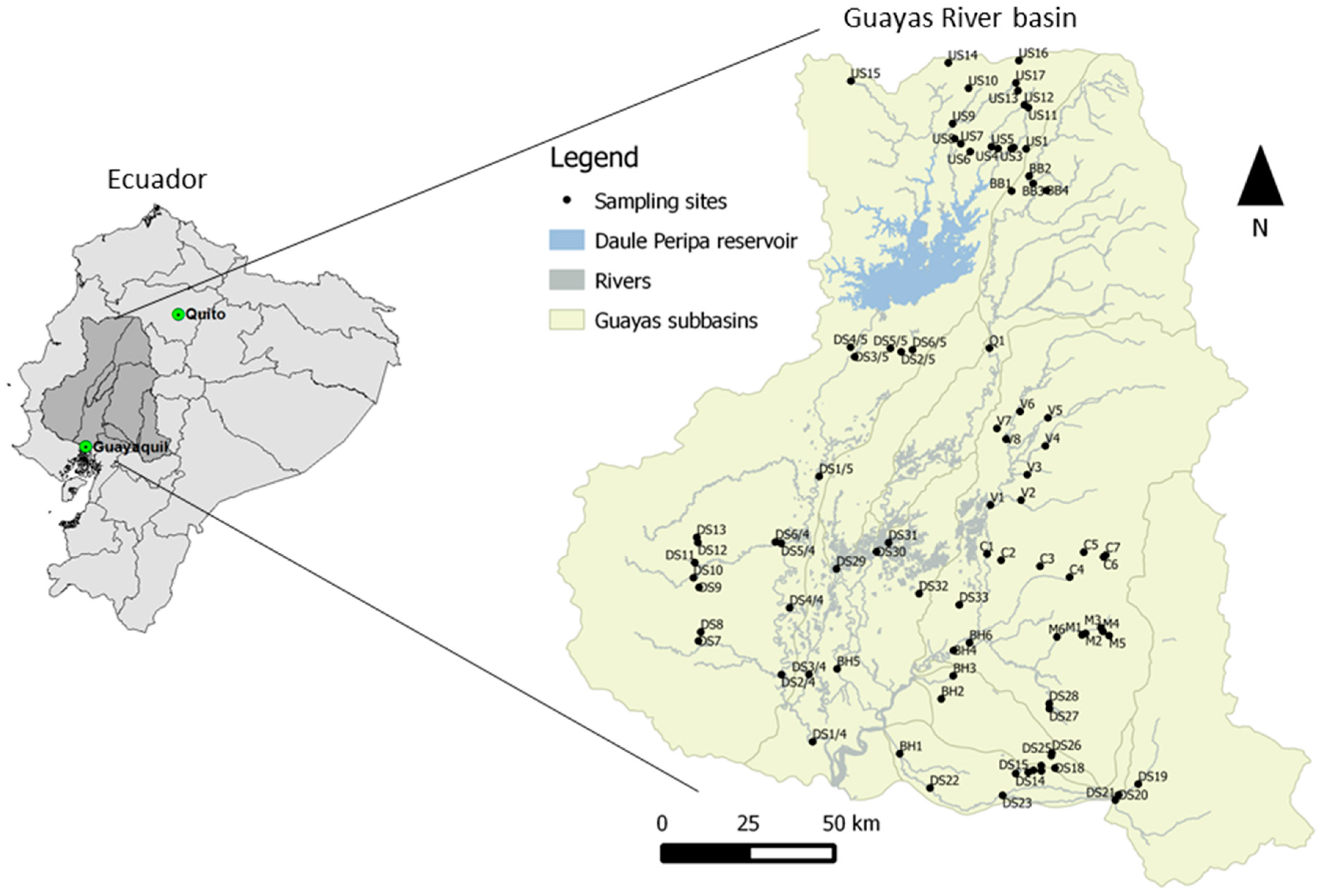
2.1. Study Area
2.2. Data Collection
2.3. Data Processing
2.3.1. Trait Allocation
2.3.2. Calculation of Functional Diversity Indices
2.4. Data Analysis
2.4.1. Response Curves
2.4.2. Determination of Tipping Points
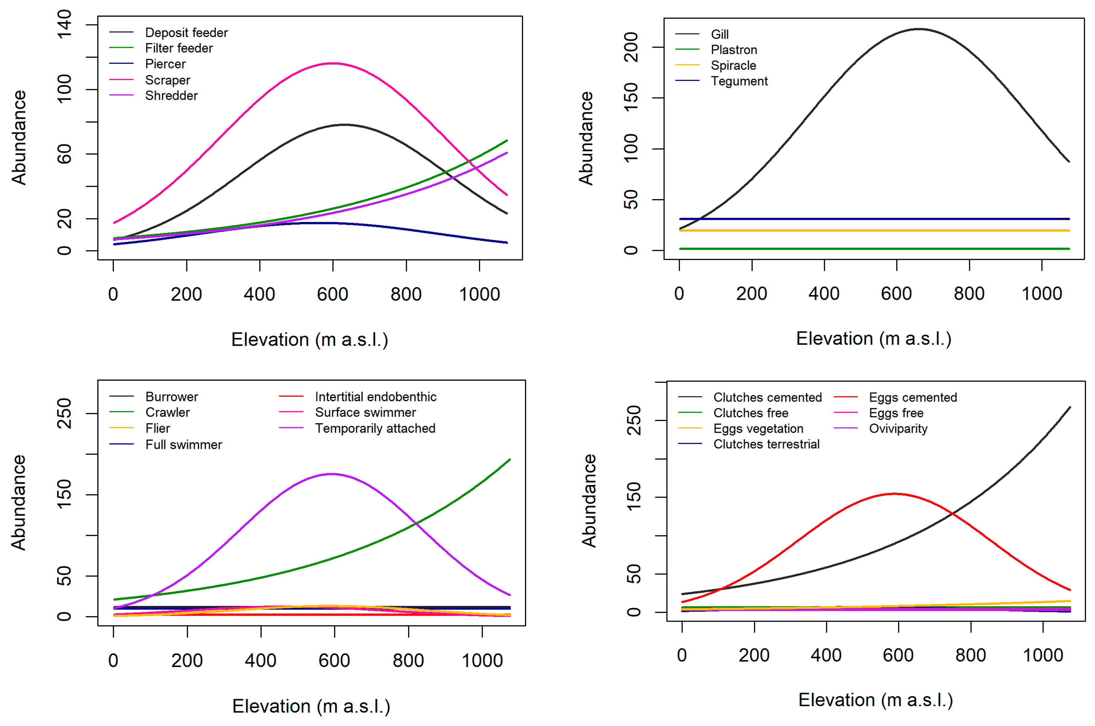
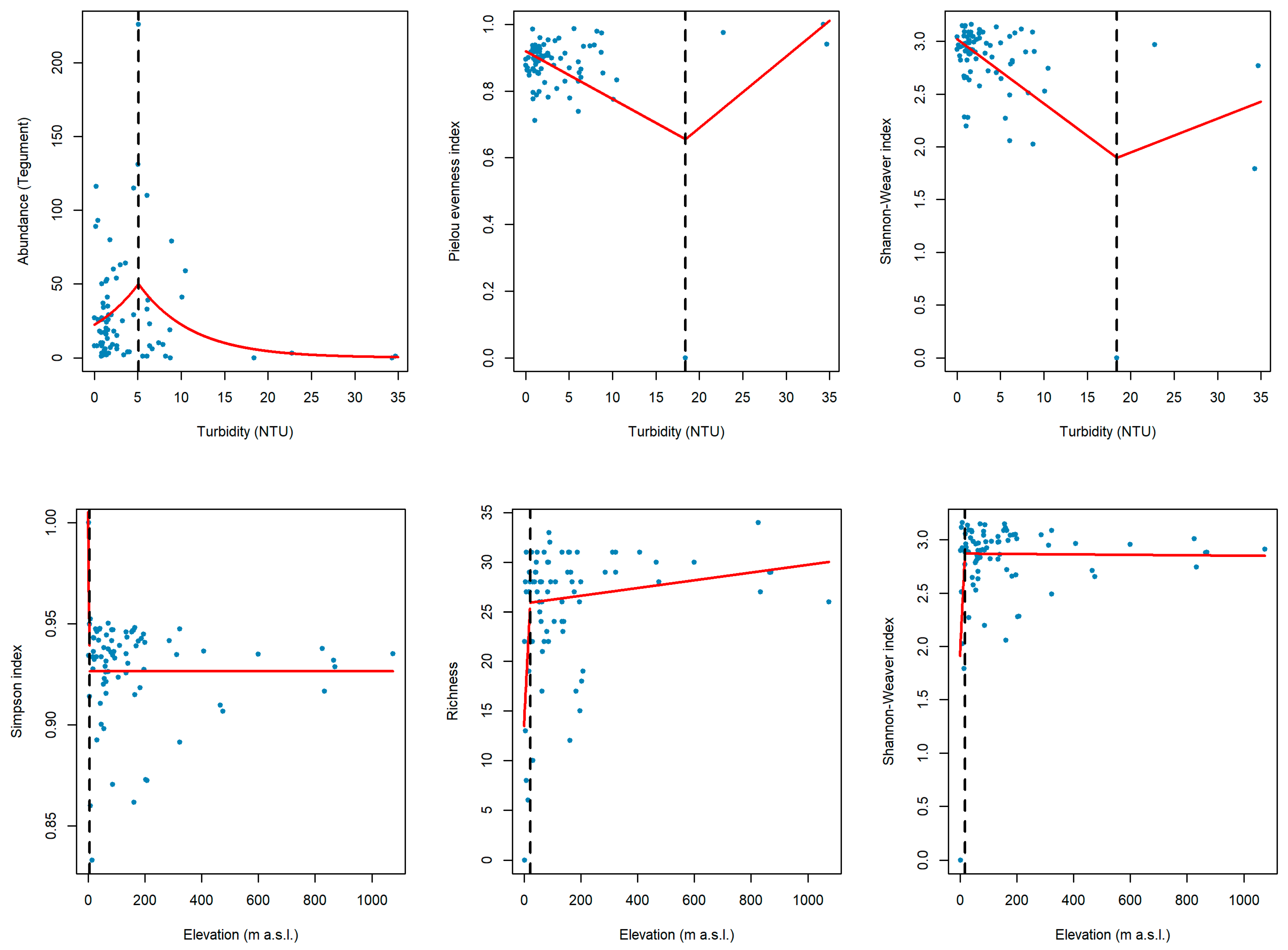
3. Results
3.1. Overview of Ecuadorian Traits Data
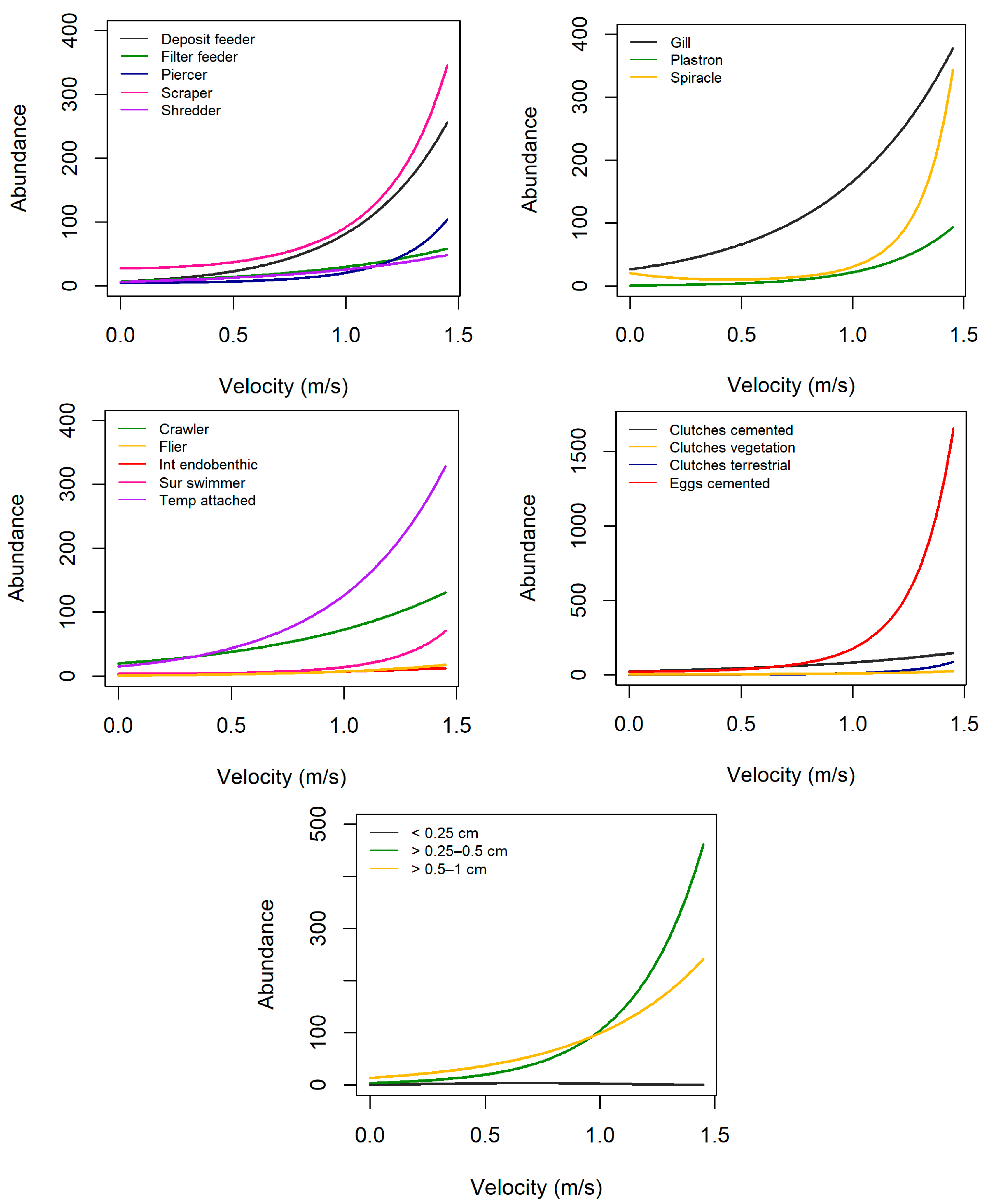
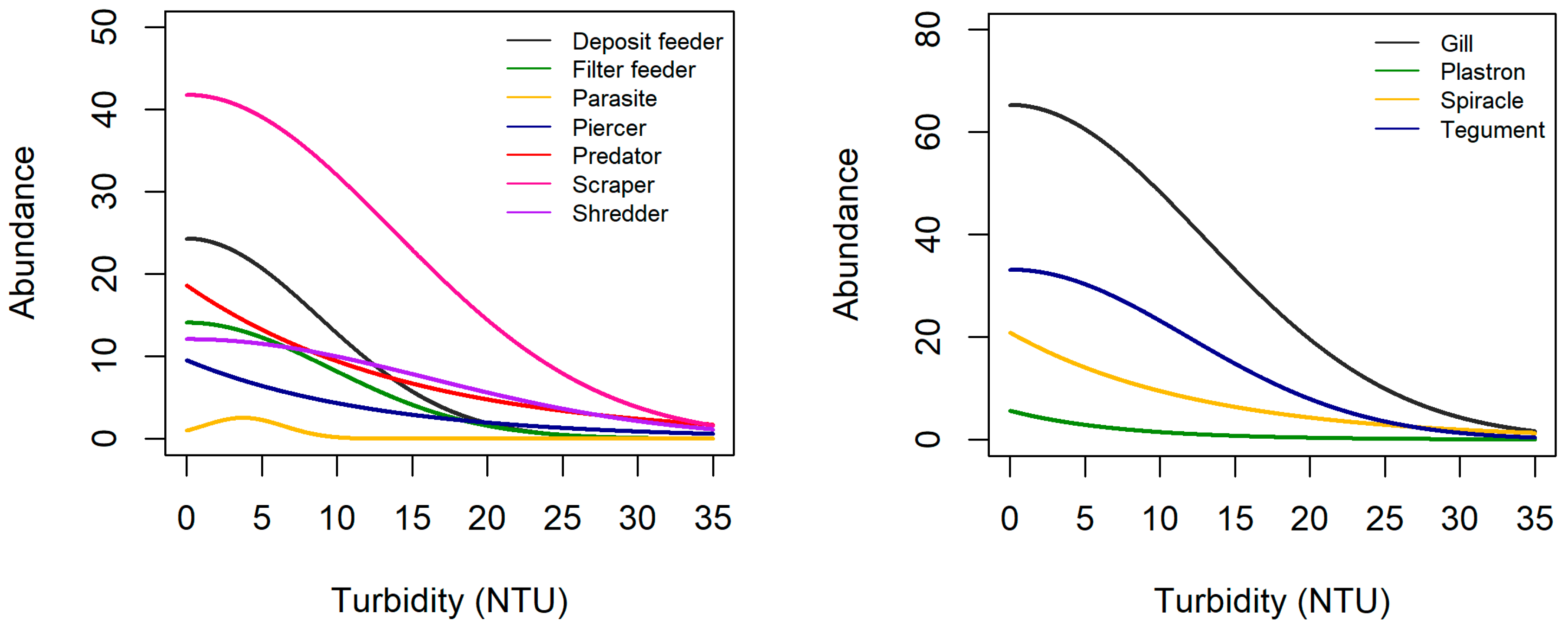
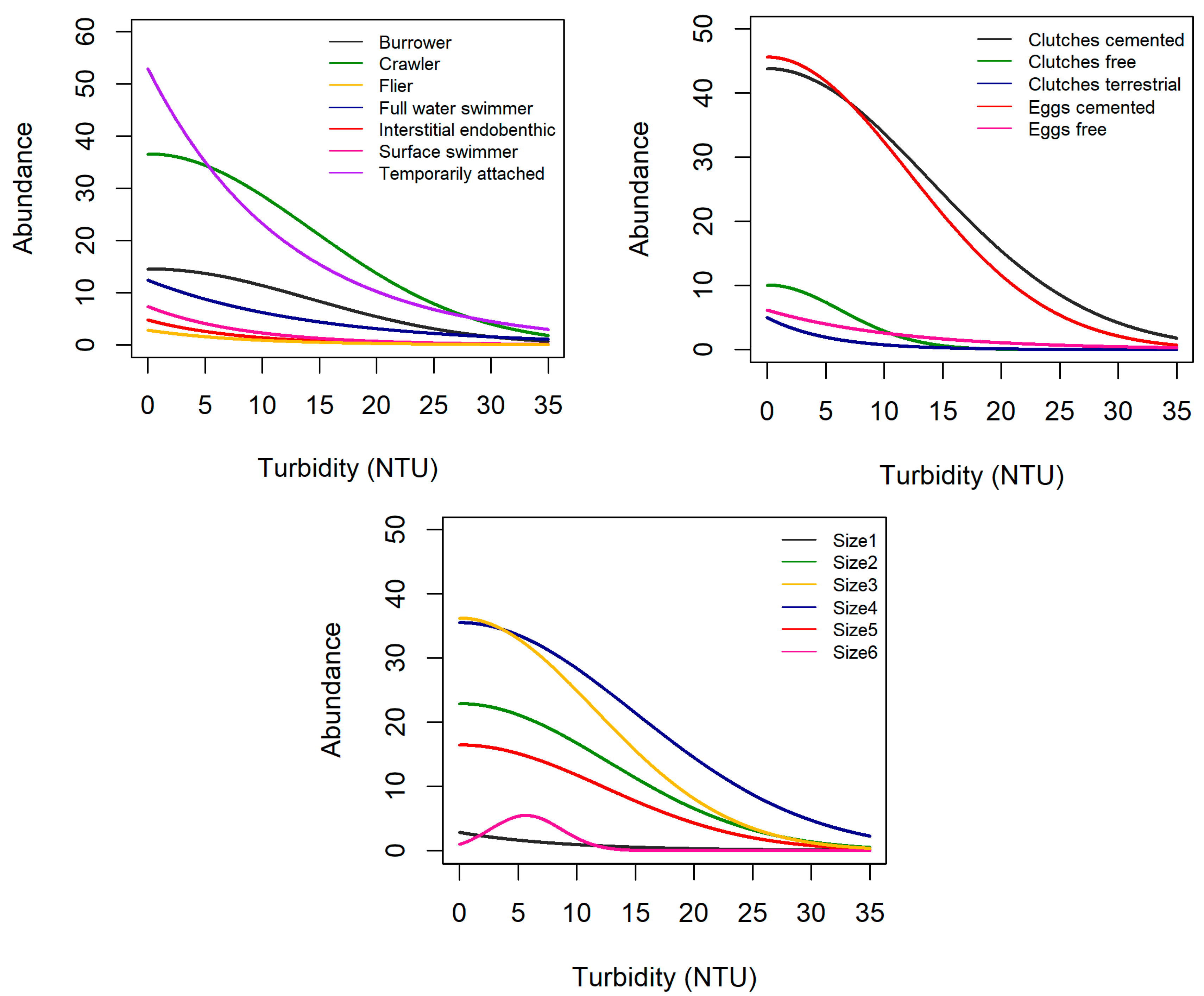
3.2. Trait Abundance Models
3.3. Tipping Points
4. Discussion
4.1. Ecological Insights
4.2. Application in Environmental Management
4.3. Tipping Points in Water Management
4.4. Implications for Further Studies
5. Conclusions
Supplementary Materials
Author Contributions
Funding
Institutional Review Board Statement
Informed Consent Statement
Data Availability Statement
Acknowledgments
Conflicts of Interest
References
- Forio, M.A.E.; Van Echelpoel, W.; Dominguez-Granda, L.; Mereta, S.T.; Ambelu, A.; Hoang, T.H.; Boets, P.; Goethals, P.L.M. Analysing the effects of water quality on the occurrence of freshwater macroinvertebrate taxa among tropical river basins from different continents. Ai Commun. 2016, 29, 665–685. [Google Scholar] [CrossRef]
- Bonada, N.; Prat, N.; Resh, V.H.; Statzner, B. Developments in aquatic insect biomonitoring: A comparative analysis of recent approaches. Annu. Rev. Entomol. 2006, 51, 495–523. [Google Scholar] [CrossRef] [PubMed] [Green Version]
- Hering, D.; Johnson, R.K.; Kramm, S.; Schmutz, S.; Szoszkiewicz, K.; Verdonschot, P.F.M. Assessment of European streams with diatoms, macrophytes, macroinvertebrates and fish: A comparative metric-based analysis of organism response to stress. Freshw. Biol. 2006, 51, 1757–1785. [Google Scholar] [CrossRef]
- Damanik-Ambarita, M.N.; Lock, K.; Boets, P.; Everaert, G.; Nguyen, T.H.T.; Forio, M.A.E.; Musonge, P.L.S.; Suhareva, N.; Bennetsen, E.; Landuyt, D.; et al. Ecological water quality analysis of the Guayas river basin (Ecuador) based on macroinvertebrates indices. Limnologica 2016, 57, 27–59. [Google Scholar] [CrossRef]
- Usseglio-Polatera, P.; Bournaud, M.; Richoux, P.; Tachet, H. Biomonitoring through biological traits of benthic macroinvertebrates: How to use species trait databases? Hydrobiologia 2000, 422, 153–162. [Google Scholar] [CrossRef]
- Poff, N.L. Landscape filters and species traits: Towards mechanistic understanding and prediction in stream ecology. J. North Am. Benthol. Soc. 1997, 16, 391–409. [Google Scholar] [CrossRef]
- Van den Brink, P.J.; Alexander, A.C.; Desrosiers, M.; Goedkoop, W.; Goethals, P.L.M.; Liess, M.; Dyer, S.D. Traits-based approaches in bioassessment and ecological risk assessment: Strengths, weaknesses, opportunities and threats. Integr. Environ. Assess. Manag. 2011, 7, 198–208. [Google Scholar] [CrossRef]
- Schmera, D.; Podani, J.; Heino, J.; Eros, T.; Poff, N.L. A proposed unified terminology of species traits in stream ecology. Freshw. Sci. 2015, 34, 823–830. [Google Scholar] [CrossRef] [Green Version]
- McGill, B.J.; Enquist, B.J.; Weiher, E.; Westoby, M. Rebuilding community ecology from functional traits. Trends Ecol. Evol. 2006, 21, 178–185. [Google Scholar] [CrossRef]
- Boets, P.; Thas, O.; Van de Vijver, E.; Lock, K.; Topke, K.; De Cooman, W.; Janssen, C.R.; Goethals, P.L.M. Relating taxonomy-based traits of macroinvertebrates with river sediment quality based on basic and zero-inflated Poisson models. Ecol. Inform. 2013, 18, 49–60. [Google Scholar] [CrossRef]
- De Lange, H.J.; Kramer, K.; Faber, J.H. Two approaches using traits to assess ecological resilience: A case study on earthworm communities. Basic Appl. Ecol. 2013, 14, 64–73. [Google Scholar] [CrossRef]
- Usseglio-Polatera, P.; Bournaud, M.; Richoux, P.; Tachet, H. Biological and ecological traits of benthic freshwater macroinvertebrates: Relationships and definition of groups with similar traits. Freshw. Biol. 2000, 43, 175–205. [Google Scholar] [CrossRef]
- van der Linden, P.; Borja, A.; Rodríquez, J.G.; Muxika, I.; Galparsoro, I.; Patrício, J.; Veríssimo, H.; Marques, J.C. Spatial and temporal response of multiple trait-based indices to natural- and anthropogenic seafloor disturbance (effluents). Ecol. Indic. 2016, 69, 617–628. [Google Scholar] [CrossRef] [Green Version]
- Mondy, C.P.; Muñoz, I.; Dolédec, S. Life-history strategies constrain invertebrate community tolerance to multiple stressors: A case study in the Ebro basin. Sci. Total Environ. 2016, 572, 196–206. [Google Scholar] [CrossRef] [PubMed]
- Jax, K. Thresholds, tipping points and limits. In OpenNESS Ecosystem Services Reference Book. EC FP7 Grant Agreement No. 308428; Potschin, M., Jax, K., Eds.; ECNC-European Centre for Nature Conservation: Tilburg, The Netherlands, 2016. [Google Scholar]
- Dodds, W.K.; Clements, W.H.; Gido, K.; Hilderbrand, R.H.; King, R.S. Thresholds, breakpoints, and nonlinearity in freshwaters as related to management. J. N. Am. Benthol. Soc. 2010, 29, 988–997. [Google Scholar] [CrossRef]
- Kelly, R.P.; Erickson, A.L.; Mease, L.A.; Battista, W.; Kittinger, J.N.; Fujita, R. Embracing thresholds for better environmental management. Philos. Trans. R. Soc. B Biol. Sci. 2015, 370, 20130276. [Google Scholar] [CrossRef] [Green Version]
- Jiang, J.; Huang, Z.-G.; Seager, T.P.; Lin, W.; Grebogi, C.; Hastings, A.; Lai, Y.-C. Predicting tipping points in mutualistic networks through dimension reduction. Proc. Natl. Acad. Sci. USA 2018, 115, E639. [Google Scholar] [CrossRef] [Green Version]
- Cai, Y.Y.; Judd, K.L.; Lenton, T.M.; Lontzek, T.S.; Narita, D. Environmental tipping points significantly affect the cost-benefit assessment of climate policies. Proc. Natl. Acad. Sci. USA 2015, 112, 4606–4611. [Google Scholar] [CrossRef] [Green Version]
- Eriksen, T.E.; Brittain, J.E.; Søli, G.; Jacobsen, D.; Goethals, P.; Friberg, N. A global perspective on the application of riverine macroinvertebrates as biological indicators in Africa, South-Central America, Mexico and Southern Asia. Ecol. Indic. 2021, 126, 107609. [Google Scholar] [CrossRef]
- Juvigny-Khenafou, N.P.D.; Piggott, J.J.; Atkinson, D.; Zhang, Y.; Macaulay, S.J.; Wu, N.; Matthaei, C.D. Impacts of multiple anthropogenic stressors on stream macroinvertebrate community composition and functional diversity. Ecol. Evol. 2021, 11, 133–152. [Google Scholar] [CrossRef]
- Manfrin, A.; Larsen, S.; Traversetti, L.; Pace, G.; Scalici, M. Longitudinal variation of macroinvertebrate communities in a Mediterranean river subjected to multiple anthropogenic stressors. Int. Rev. Hydrobiol. 2013, 98, 155–164. [Google Scholar] [CrossRef]
- Sotomayor, G.; Hampel, H.; Vázquez, R.F.; Forio, M.A.E.; Goethals, P.L.M. Implications of macroinvertebrate taxonomic resolution for freshwater assessments using functional traits: The Paute River Basin (Ecuador) case. Divers. Distrib. 2021, 28, 1735–1747. [Google Scholar] [CrossRef]
- Mercado-Garcia, D.; Beeckman, E.; Van Butsel, J.; Deza Arroyo, N.; Sanchez Peña, M.; Forio, M.A.E.; De Schamphelaere Karel, A.C.; Wyseure, G.; Goethals, P. Freshwater macroinvertebrate traits assessment as complementary to taxonomic information for mining impact detection in the northern Peruvian Andes. Divers. Distrib. 2022, 28, 1582–1596. [Google Scholar] [CrossRef]
- Monk, W.A.; Compson, Z.G.; Armanini, D.G.; Orlofske, J.M.; Curry, C.J.; Peters, D.L.; Crocker, J.B.; Baird, D.J. Flow velocity-ecology thresholds in Canadian rivers: A comparison of trait and taxonomy-based approaches. Freshw. Biol. 2018, 63, 891–905. [Google Scholar] [CrossRef]
- Folegot, S.; Bruno, M.C.; Larsen, S.; Kaffas, K.; Pisaturo, G.R.; Andreoli, A.; Comiti, F.; Maurizio, R. The effects of a sediment flushing on Alpine macroinvertebrate communities. Hydrobiologia 2021, 848, 3921–3941. [Google Scholar] [CrossRef]
- Calapez, A.R.; Serra, S.R.Q.; Santos, J.M.; Branco, P.; Ferreira, T.; Hein, T.; Brito, A.G.; Feio, M.J. The effect of hypoxia and flow decrease in macroinvertebrate functional responses: A trait-based approach to multiple-stressors in mesocosms. Sci. Total Environ. 2018, 637–638, 647–656. [Google Scholar] [CrossRef] [PubMed]
- Damanik-Ambarita, M.N.; Everaert, G.; Forio, M.A.E.; Nguyen, T.H.T.; Lock, K.; Musonge, P.L.S.; Suhareva, N.; Dominguez-Granda, L.; Bennetsen, E.; Boets, P.; et al. Generalized linear models to identify key hydromorphological and chemical variables determining the occurrence of macroinvertebrates in the Guayas river basin (Ecuador). Water-Sui 2016, 8, 297. [Google Scholar] [CrossRef] [Green Version]
- Forio, M.A.E.; Mouton, A.; Lock, K.; Boets, P.; Nguyen, T.H.T.; Damanik Ambarita, M.N.; Musonge, P.L.S.; Dominguez-Granda, L.; Goethals, P.L.M. Fuzzy modelling to identify key drivers of ecological water quality to support decision and policy making. Environ. Sci. Policy 2017, 68, 58–68. [Google Scholar] [CrossRef]
- Heino, J. Functional biodiversity of macroinvertebrate assemblages along major ecological gradients of boreal headwater streams. Freshw. Biol. 2005, 50, 1578–1587. [Google Scholar] [CrossRef]
- Vannote, R.L.; Minshall, G.W.; Cummins, K.W.; Sedell, J.R.; Cushing, C.E. River Continuum Concept. Can. J. Fish. Aquat. Sci. 1980, 37, 130–137. [Google Scholar] [CrossRef]
- Brooks, A.J.; Haeusler, T. Invertebrate responses to flow: Trait-velocity relationships during low and moderate flows. Hydrobiologia 2016, 773, 23–34. [Google Scholar] [CrossRef]
- Fuller, R.L.; Griego, C.; Muehlbauer, J.D.; Dennison, J.; Doyle, M.W. Response of stream macroinvertebrates in flow refugia and high-scour areas to a series of floods: A reciprocal replacement study. J. N. Am. Benthol. Soc. 2010, 29, 750–760. [Google Scholar] [CrossRef]
- Jowett, I.G.; Biggs, B.J.F. Flood and velocity effects on periphyton and silt accumulation in two New Zealand rivers. N. Z. J. Mar. Freshw. Res. 1997, 31, 287–300. [Google Scholar] [CrossRef]
- Statzner, B.; Bêche, L. Can biological invertebrate traits resolve effects of multiple stressors on running water ecosystems? Freshw. Biol. 2010, 55, 80–119. [Google Scholar] [CrossRef]
- Vogel, S. Life in Moving Fluids The Physical Biology of Flow—Revised and Expanded Second Edition, NED—New Edition; Princeton University Press: Princeton, NJ, USA, 1994. [Google Scholar]
- Statzner, B.; Bonada, N.; Doledec, S. Predicting the abundance of European stream macroinvertebrates using biological attributes. Oecologia 2008, 156, 65–73. [Google Scholar] [CrossRef] [PubMed]
- Horrigan, N.; Baird, D.J. Trait patterns of aquatic insects across gradients of flow-related factors: A multivariate analysis of Canadian national data. Can. J. Fish. Aquat. Sci. 2008, 65, 670–680. [Google Scholar] [CrossRef]
- Jones, F.C. Taxonomic sufficiency: The influence of taxonomic resolution on freshwater bioassessments using benthic macroinvertebrates. Environ. Rev. 2008, 16, 45–69. [Google Scholar] [CrossRef]
- Rezende, R.S.; Santos, A.M.; Henke-Oliveira, C.; Goncalves, J.F. Effects of spatial and environmental factors on benthic a macroinvertebrate community. Zoologia 2014, 31, 426–434. [Google Scholar] [CrossRef] [Green Version]
- Feio, M.J.; Ferreira, W.R.; Macedo, D.R.; Eller, A.P.; Alves, C.B.M.; Franca, J.S.; Callisto, M. Defining and testing targets for the recovery of tropical streams based on macroinvertebrate communities and abiotic conditions. River Res. Appl. 2015, 31, 70–84. [Google Scholar] [CrossRef]
- Statzner, B.; Doledec, S.; Hugueny, B. Biological trait composition of European stream invertebrate assemblages: Assessing the effects of various trait filter types. Ecogeography 2004, 27, 470–488. [Google Scholar] [CrossRef]
- Townsend, C.R.; Hildrew, A.G. Species traits in relation to a habitat templet for river systems. Freshw. Biol. 1994, 31, 265–275. [Google Scholar] [CrossRef]
- Nguyen, T.H.T.; Boets, P.; Lock, K.; Ambarita, M.N.D.; Forio, M.A.E.; Sasha, P.; Dominguez-Granda, L.E.; Hoang, T.H.T.; Everaert, G.; Goethals, P.L.M. Habitat suitability of the invasive water hyacinth and its relation to water quality and macroinvertebrate diversity in a tropical reservoir. Limnologica 2015, 52, 67–74. [Google Scholar] [CrossRef]
- Frappart, F.; Bourrel, L.; Brodu, N.; Riofrío Salazar, X.; Baup, F.; Darrozes, J.; Pombosa, R. Monitoring of the spatio-temporal dynamics of the floods in the Guayas watershed (Ecuadorian Pacific Coast) using global monitoring ENVISAT ASAR images and rainfall data. Water 2017, 9, 12. [Google Scholar] [CrossRef] [Green Version]
- Gabriels, W.; Lock, K.; De Pauw, N.; Goethals, P.L.M. Multimetric Macroinvertebrate Index Flanders (MMIF) for biological assessment of rivers and lakes in Flanders (Belgium). Limnologica 2010, 40, 199–207. [Google Scholar] [CrossRef] [Green Version]
- De Pauw, N.; Van Damme, D.; Vaate, B.D. Manual for Macroinvertebrate Identification and Water Quality Assessment, Integrated Programme for Implementation of the Recommended Transnational Monitoring Strategy for the Danube River Basin, CEC PHARE/TACIS Project; Ghent University: Ghent, Belgium, 1996. [Google Scholar]
- Dominguez, E.; Fernández, H.R. Macroinvertebrados Bentoınicos Sudamericanos: Sistemática y Biologia; Fundacio´ın Miguel Lillo: Tucumán, Argentina, 2009. [Google Scholar]
- Tachet, H.; Richoux, P.; Bournaud, M.; Usseglio-Polatera, P. Invertêbrés d’Eau Douce:Systématique, Biologie, Écologie; CNRS éditions: Paris, France, 2000. [Google Scholar]
- Forio, M.A.E.; Goethals, P.L.M.; Lock, K.; Asio, V.; Bande, M.; Thas, O. Model-based analysis of the relationship between macroinvertebrate traits and environmental river conditions. Environ. Model. Softw. 2018, 106, 57–67. [Google Scholar] [CrossRef]
- Jari Oksanen, F.; Blanchet, G.; Friendly, M.; Kindt, R.; Legendre, P.; McGlinn, D.; Minchin, P.R.; O’Hara, R.B.; Simpson, G.L.; Solymos, P.; et al. Vegan: Community Ecology Package. R Package Version 2.5-2; University of Auckland: Auckland, New Zealand, 2022. [Google Scholar]
- Forio, M.A.E. Statistical Analysis of Stream Invertebrate Traits in Relation to River Conditions. Ph.D. Thesis, Ghent University, Ghent, Belgium, 2017. [Google Scholar]
- Zuur, A.F.; Ieno, E.N.; Elphick, C.S. A protocol for data exploration to avoid common statistical problems. Methods Ecol. Evol. 2010, 1, 3–14. [Google Scholar] [CrossRef]
- Zuur, A.F.; Ieno, E.N.; Walker, N.J.; Saveliev, A.A.; Smith, G.M. Mixed Effects Models and Extensions Ion Ecology with R; Springer Science+Business Media, LLC 2009: New York, NY, USA, 2009. [Google Scholar]
- R Core Team. R: A Language and Environment for Statistical Computing R Foundation for Statistical Computing, Vienna, Austria. 2016. Available online: https://www.R-project.org/ (accessed on 12 August 2021).
- Venables, W.N.; Ripley, B.D. Modern Applied Statistics with S, 4th ed.; Springer: New York, NY, USA, 2002. [Google Scholar]
- Vanacker, M.; Wezel, A.; Payet, V.; Robin, J. Determining tipping points in aquatic ecosystems: The case of biodiversity and chlorophyll α relations in fish pond systems. Ecol. Indic. 2015, 52, 184–193. [Google Scholar] [CrossRef]
- Muggeo, V.M.R. Segmented: An R package to fit regression models with broken-line relationships. R News 2008, 8, 20–25. [Google Scholar]
- Davies, R.B. Hypothesis testing when a nuisance parameter is present only under the alternatives. Biometrika 1987, 74, 33–43. [Google Scholar] [CrossRef]
- Muggeo, V.M.R. Testing with a nuisance parameter present only under the alternative: A score-based approach with application to segmented modelling. J. Stat. Comput. Simul. 2016, 86, 3059–3067. [Google Scholar] [CrossRef]
- Dewson, Z.S.; James, A.B.W.; Death, R.G. A review of the consequences of decreased flow for instream habitat and macroinvertebrates. J. North Am. Benthol. Soc. 2007, 26, 401–415. [Google Scholar] [CrossRef]
- Elbrecht, V.; Beermann, A.J.; Goessler, G.; Neumann, J.; Tollrian, R.; Wagner, R.; Wlecklik, A.; Piggott, J.J.; Matthaei, C.D.; Leese, F. Multiple-stressor effects on stream invertebrates: A mesocosm experiment manipulating nutrients, fine sediment and flow velocity. Freshw. Biol. 2016, 61, 362–375. [Google Scholar] [CrossRef]
- Forio, M.A.E.; Landuyt, D.; Bennetsen, E.; Lock, K.; Nguyen, T.H.T.; Ambarita, M.N.D.; Musonge, P.L.S.; Boets, P.; Everaert, G.; Dominguez-Granda, L.; et al. Bayesian belief network models to analyse and predict ecological water quality in rivers. Ecol. Model. 2015, 312, 222–238. [Google Scholar] [CrossRef]
- Brooks, A.J.; Chessman, B.C.; Haeusler, T. Macroinvertebrate traits distinguish unregulated rivers subject to water abstraction. J. N. Am. Benthol. Soc. 2011, 30, 419–435. [Google Scholar] [CrossRef]
- Lancaster, J.; Downes, B. Linking the hydraulic world of individual organisms to ecological processes: Putting ecology into ecohydraulics. River Res. Appl. 2010, 26, 385–403. [Google Scholar] [CrossRef]
- Biggs, C.R.; Yeager, L.A.; Bolser, D.G.; Bonsell, C.; Dichiera, A.M.; Hou, Z.; Keyser, S.R.; Khursigara, A.J.; Lu, K.; Muth, A.F.; et al. Does functional redundancy affect ecological stability and resilience? A review and meta-analysis. Ecosphere 2020, 11, e03184. [Google Scholar] [CrossRef]
- Cabrera, S.; Forio, M.A.E.; Lock, K.; Vandenbroucke, M.; Oña, T.; Gualoto, M.; Goethals, P.L.M.; Van der heyden, C. Variations in benthic macroinvertebrate communities and biological quality in the Aguarico and Coca river basins in the Ecuadorian Amazon. Water 2021, 13, 1692. [Google Scholar] [CrossRef]
- Forio, M.A.E.; Lock, K.; Radam, E.D.; Bande, M.; Asio, V.; Goethals, P. Assessment and analysis of ecological quality, macroinvertebrate communities and diversity in rivers of a multifunctional tropical island. Ecol. Indic. 2017, 77, 228–238. [Google Scholar] [CrossRef]
- Munyika, S.; Kongo, V.; Kimwaga, R. River health assessment using macroinvertebrates and water quality parameters: A case of the Orange River in Namibia. Phys. Chem. Earth Parts A/B/C 2014, 76–78, 140–148. [Google Scholar] [CrossRef]
- USEPA. Volunteer Stream Monitoring: A Methods Manual. Available online: http://www.water-research.net/Waterlibrary/Lake/STREAM.PDF (accessed on 19 November 2018).
- Jones, J.I.; Murphy, J.F.; Collins, A.L.; Sear, D.A.; Naden, P.S.; Armitage, P.D. The impact of fine sediment on macroinvertebrates. River Res. Appl. 2012, 28, 1055–1071. [Google Scholar] [CrossRef]
- Wagenhoff, A.; Townsend, C.R.; Matthaei, C.D. Macroinvertebrate responses along broad stressor gradients of deposited fine sediment and dissolved nutrients: A stream mesocosm experiment. J. Appl. Ecol. 2012, 49, 892–902. [Google Scholar] [CrossRef]
- Wood, P.J.; Armitage, P.D. Biological effects of fine sediment in the lotic environment. Environ. Manag. 1997, 21, 203–217. [Google Scholar] [CrossRef] [PubMed]
- Matthaei, C.D.; Piggott, J.J.; Townsend, C.R. Multiple stressors in agricultural streams: Interactions among sediment addition, nutrient enrichment and water abstraction. J. Appl. Ecol. 2010, 47, 639–649. [Google Scholar] [CrossRef]
- Ntloko, P.; Palmer, C.G.; Akamagwuna, F.C.; Odume, O.N. Exploring macroinvertebrates ecological preferences and trait-based indicators of suspended fine sediment effects in the Tsitsa River and its tributaries, Eastern Cape, South Africa. Water 2021, 13, 798. [Google Scholar] [CrossRef]
- Laura, M.M.; Adriana, M.K.; Cecilia, B.; La Ludmila, M.; Di Cecilia, P.Y.; Gabriela, P.; Jose, B. Ecological status of a Patagonian mountain river: Usefulness of environmental and biotic metrics for rehabilitation assessment. Environ. Manag. 2016, 57, 1166–1187. [Google Scholar] [CrossRef]
- Eddy, E.N.; Roman, C.T. Relationship between epibenthic invertebrate species assemblages and environmental variables in Boston harbor’s intertidal habitat. Northeast. Nat. 2016, 23, 45–66. [Google Scholar] [CrossRef]
- Mauad, M.; Miserendino, M.L.; Risso, M.A.; Massaferro, J. Assessing the performance of macroinvertebrate metrics in the Challhuaco-Nireco System (Northern Patagonia, Argentina). Iheringia Ser. Zool. 2015, 105, 348–358. [Google Scholar] [CrossRef] [Green Version]
- Lang, C.; Reymond, O. Empirical relationships between diversity of invertebrate communities and altitude in rivers—Application to biomonitoring. Aquat. Sci. 1993, 55, 188–196. [Google Scholar] [CrossRef]
- Montano-Centellas, F.A.; Garitano-Zavala, A. Andean bird responses to human disturbances along an elevational gradient. Acta Oecologica-Int. J. Ecol. 2015, 65–66, 51–60. [Google Scholar] [CrossRef]
- Vasquez, D.L.A.; Balslev, H.; Sklenar, P. Human impact on tropical-alpine plant diversity in the northern Andes. Biodivers. Conserv. 2015, 24, 2673–2683. [Google Scholar] [CrossRef]
- Corkum, L.; Pointing, P.; Ciborowski, J. Influence of current velocity and substrate on distribution and drift of 2 species of mayflies (Ephemeroptera). Can. J. Zool. 1977, 55, 1970–1977. [Google Scholar] [CrossRef]
- U.S. Environmental Protection Agency. National Management Measures to Control Nonpoint Source Pollution from Agriculture; U.S. Environmental Protection Agency Office of Water: Washington, DC, USA, 2003.
- Forio, M.A.E.; Burdon, F.J.; De Troyer, N.; Lock, K.; Witing, F.; Baert, L.; De Saeyer, N.; Rîșnoveanu, G.; Popescu, C.; Kupilas, B.; et al. A Bayesian Belief Network learning tool integrates multi-scale effects of riparian buffers on stream invertebrates. Sci. Total Environ. 2022, 810, 152146. [Google Scholar] [CrossRef]
- Zeileis, A.; Leisch, F.; Hornik, K.; Kleiber, C. strucchange: An R Package for Testing for Structural Change in Linear Regression Models. J. Stat. Softw. 2002, 7, 38. [Google Scholar] [CrossRef] [Green Version]
- Robin, J.; Wezel, A.; Bornette, G.; Arthaud, F.; Angélibert, S.; Rosset, V.; Oertli, B. Biodiversity in eutrophicated shallow lakes: Determination of tipping points and tools for monitoring. Hydrobiologia 2014, 723, 63–75. [Google Scholar] [CrossRef]
- Baker, M.E.; King, R.S. A new method for detecting and interpreting biodiversity and ecological community thresholds. Methods Ecol. Evol. 2010, 1, 25–37. [Google Scholar] [CrossRef]
- King, R.S.; Baker, M.E. Use, Misuse, and Limitations of Threshold Indicator Taxa Analysis (TITAN) for Natural Resource Management. In Application of Threshold Concepts in Natural Resource Decision Making; Guntenspergen, G.R., Ed.; Springer: New York, NY, USA, 2014. [Google Scholar]
- Mouton, A.M.; Dedecker, A.P.; Lek, S.; Goethals, P.L.M. Selecting variables for habitat suitability of Asellus (Crustacea, Isopoda) by applying input variable contribution methods to artificial neural network models. Environ. Model. Assess. 2010, 15, 65–79. [Google Scholar] [CrossRef]
- Groffman, P.; Baron, J.; Blett, T.; Gold, A.; Goodman, I.; Gunderson, L.; Levinson, B.; Palmer, M.; Paerl, H.; Peterson, G.; et al. Ecological thresholds: The key to successful environmental management or an important concept with no practical application? Ecosystems 2006, 9, 1–13. [Google Scholar] [CrossRef]
- Heino, J.; Schmera, D.; Eros, T. A macroecological perspective of trait patterns in stream communities. Freshw. Biol. 2013, 58, 1539–1555. [Google Scholar] [CrossRef] [Green Version]
- Besacier Monbertrand, A.-L.; Timoner, P.; Rahman, K.; Burlando, P.; Fatichi, S.; Gonseth, Y.; Moser, F.; Castella, E.; Lehmann, A. Assessing the vulnerability of aquatic macroinvertebrates to climate warming in a mountainous watershed: Supplementing presence-only data with species traits. Water 2019, 11, 636. [Google Scholar] [CrossRef] [Green Version]
- Soininen, J.; Kononen, K. Comparative study of monitoring South-Finnish rivers and streams using macroinvertebrate and benthic diatom community structure. Aquat. Ecol. 2004, 38, 63–75. [Google Scholar] [CrossRef]
- Twardochleb, L.; Hiltner, E.; Pyne, M.; Zarnetske, P. Freshwater insects CONUS: A database of freshwater insect occurrences and traits for the contiguous United States. Glob. Ecol. Biogeogr. 2021, 30, 826–841. [Google Scholar] [CrossRef] [PubMed]
- De Oliveira, S.S.; Ortega, J.C.G.; Ribas, L.G.D.; Lopes, V.G.; Bini, L.M. Higher taxa are sufficient to represent biodiversity patterns. Ecol. Indic. 2020, 111, 105994. [Google Scholar] [CrossRef]
- Gayraud, S.; Statzner, B.; Bady, P.; Haybachp, A.; Scholl, F.; Usseglio-Polatera, P.; Bacchi, M. Invertebrate traits for the biomonitoring of large European rivers: An initial assessment of alternative metrics. Freshw. Biol. 2003, 48, 2045–2064. [Google Scholar] [CrossRef] [Green Version]
- Doledec, S.; Statzner, B. Responses of freshwater biota to human disturbances: Contribution of J-NABS to developments in ecological integrity assessments. J. N. Am. Benthol. Soc. 2010, 29, 286–311. [Google Scholar] [CrossRef]
- Conti, L.; Schmidt-Kloiber, A.; Grenouillet, G.; Graf, W. A trait-based approach to assess the vulnerability of European aquatic insects to climate change. Hydrobiologia 2014, 721, 297–315. [Google Scholar] [CrossRef] [Green Version]
- Vannevel, R.; Goethals, P.L.M. Identifying ecosystem key factors to support sustainable water management. Sustainability 2020, 12, 1148. [Google Scholar] [CrossRef] [Green Version]
- Forio, M.A.; Goethals, P.L.M. An integrated approach of multi-community monitoring and assessment of aquatic ecosystems to support sustainable development. Sustainability 2020, 12, 5603. [Google Scholar] [CrossRef]
- Schmera, D.; Heino, J.; Podani, J.; Erős, T.; Dolédec, S. Functional diversity: A review of methodology and current knowledge in freshwater macroinvertebrate research. Hydrobiologia 2017, 787, 27–44. [Google Scholar] [CrossRef] [Green Version]
- Schäfer, R.B.; Kefford, B.; Metzeling, L.; Liess, M.; Burgert, S.; Marchant, R.; Pettigrove, V.; Goonan, P.; Nugegoda, D. A trait database of stream invertebrates for the ecological risk assessment of single and combined effects of salinity and pesticides in South-East Australia. Sci. Total Environ. 2011, 409, 2055–2063. [Google Scholar] [CrossRef]
- Schuwirth, N.; Kattwinkel, M.; Stamm, C. How stressor specific are trait-based ecological indices for ecosystem management? Sci. Total Environ. 2015, 505, 565–572. [Google Scholar] [CrossRef] [Green Version]
- Van Echelpoel, W.; Forio, A.M.; Van der heyden, C.; Bermúdez, R.; Ho, L.; Rosado Moncayo, M.A.; Parra Narea, N.R.; Dominguez Granda, E.L.; Sanchez, D.; Goethals, L.P. Spatial characteristics and temporal evolution of chemical and biological freshwater status as baseline assessment on the tropical island San Cristóbal (Galapagos, Ecuador). Water-Sui 2019, 11, 880. [Google Scholar] [CrossRef] [Green Version]
- Van Echelpoel, W.; Forio, M.A.E.; Van Butsel, J.; Lock, K.; Utreras, J.A.D.; Dominguez-Granda, L.E.; Goethals, P.L.M. Macroinvertebrate functional feeding group structure along an impacted tropical river: The Portoviejo River (Ecuador). Limnologica 2018, 73, 12–19. [Google Scholar] [CrossRef]
- Brandt, D. Temperature Preferences and Tolerances for 137 Common Idaho Macroinvertebrate Taxa; Idaho Department of Environmental Quality: Boise, ID, USA, 2001.
- EPA GCRP Maine. EPA GCRP State Biomonitoring Data Climate Change Pilot Project 2010: Freshwater Biological Traits Table for Maine; Global Change Research Program: Washington, DC, USA, 2010.
- EPA GCRP North Carolina. EPA GCRP State Biomonitoring Data Climate Change Pilot Project 2010: Freshwater Biological Traits Table for North Carolina; Global Change Research Program: Washington, DC, USA, 2010.
- EPA GCRP Utah. EPA GCRP State Biomonitoring Data Climate Change Pilot Project 2010: Freshwater Biological Traits Table for Utah; Global Change Research Program: Washington, DC, USA, 2010.
- Hubbard, M.D.; Peters, W.L. Environmental Requirements and Pollution Tolerance of Ephemeroptera; US EPA Environmental Monitoring and Support Laboratory: Cincinnati, OH, USA, 1978. [Google Scholar]
- Huff, D.D.; Hubler, S.L.; Pan, Y.; Drake, D.L. Detecting Shifts in Macroinvertebrate Community Requirements: Implicating Causes of Impairment in Streams; Oregon Department of Environmental Quali: Portland, OR, USA, 2008.
- MarLIN. BIOTIC—Biological Traits Information Catalogue Marine Life Information Network Plymouth; Marine Biological Association of the United Kingdom: Plymouth, UK, 2006. [Google Scholar]
- Poff, N.L.; Olden, J.D.; Vieira, N.K.; Finn, D.S.; Simmons, M.P.; Kondratieff, B.C. Functional trait niches of North American lotic insects: Traits-based ecological applications in light of phylogenetic relationships. J. N. Am. Benthol. Soc. 2006, 25, 730–755. [Google Scholar] [CrossRef] [Green Version]
- Rankin, E.T.; Yoder, C.O. Temporal Change in Regional Reference Condition as a Potential Indicator of Global Climate Change: Analysis of the Ohio Regional Reference Condition Database (1980–2006); Midwest Biodiversity Institute: Hilliard, OH, USA, 2009. [Google Scholar]
- Schmidt-Kloiber, A.; Hering, D. Online Tool That Unifies, Standardises and Codifies More than 20,000 European Freshwater Organisms and Their Ecological Preferences. Ecol. Indic. 2015, 53, 271–282. [Google Scholar] [CrossRef]
- Tomanova, S.; Moya, N.; Oberdorff, T. Using Macroinvertebrate Biological Traits for Assessing Biotic Integrity of Neotropical Streams. River Res. Appl. 2008, 24, 1230–1239. [Google Scholar] [CrossRef]
- USEPA. Traits—Data Sources and Metadata; U.S. Environmental Protection Agency: Washington, DC, USA, 2008.
- Vieira, N.K.M.; Poff, N.L.; Carlisle, D.M.; Moulton, S.R., II.; Koski, M.K.; Kondratieff, B.C. A Database of Lotic Invertebrate Traits for North America; U.S. Geological Survey: Reston, VA, USA, 2006.


| Grouping Features | Traits | Velocity (+) | Turbidity (+) | Elevation (+) |
|---|---|---|---|---|
| Feeding style | Deposit feeder | – | + | h |
| Filter feeder | + | – | h | |
| Parasite | nr | nr | nr | |
| Piercer | nr | nr | h | |
| Predator | – | – | ↑-> mid, C after mid | |
| Scraper/grazer | + | – | h | |
| Shredder | – | – | + | |
| Locomotion | Burrower | nr | + | – |
| Crawler | + | – | + | |
| Flier | nr | – | ↑-> mid, C after mid | |
| Full water swimmer | – | – | ↑-> mid, C after mid | |
| Instertitial (endobenthic) | nr | nr | nr | |
| Surface swimmer | – | nr | ↑-> mid, C after mid | |
| Temporary attached | nr | – | h | |
| Reproduction | Clutches, cemented | + | – | + |
| Clutches, free | – | – | h | |
| Clutches in vegetation | nr | – | L -> low | |
| Clutches, terrestrial | nr | nr | L -> low | |
| Isolated eggs, cemented | + | – | + | |
| Isolated eggs, free | – | – | h | |
| Oviviparity | nr | nr | L -> low | |
| Respiration | Gills | + | – | + |
| Hydrostatic vesicle | nr | nr | nr | |
| Plastron | nr | – | nr | |
| Spiracle | nr | nr | nr | |
| Tegument | + | – | + | |
| Maximal potential size | Size1 (≤0.25 cm) | + | nr | + |
| Size2 (>0.25–0.5 cm) | + | nr | + | |
| Size3 (>0.5–1 cm) | + | – | h | |
| Size4 (>1–2 cm) | + | – | h | |
| Size5 (>2–4 cm) | nr | – | h | |
| Size6 (>4–8 cm) | nr | – | h | |
| Size7 (>8 cm) | nr | – | – |
| Unit | Mean | Median | Min. | Max. | Standard Deviation | |
|---|---|---|---|---|---|---|
| Elevation | m a.s.l. | 166 | 86 | 2.0 | 1075 | 222 |
| Velocity | m/s | 0.3 | 0.3 | 0.0 | 1.5 | 0.29 |
| Turbidity | NTU | 4.2 | 2.0 | 0.0 | 34.7 | 6.2 |
| Grouping Features | Traits |
|---|---|
| Feeding style | Absorber, deposit feeder, filter feeder, parasite, piercer, predator, scraper, shredder |
| Respiration mode | Gill, plastron, spiracle, tegument |
| Locomotion mode | Burrower, crawler, flier, full water swimmer, interstitial endobenthic, surface swimmer, temporarily attached |
| Reproduction mode | Clutches cemented, clutches free, clutches terrestrial, clutches in vegetation, isolated eggs cemented, isolated eggs free, oviviparity |
| Sizes | Size1 (≤0.25 cm), size2 (>0.25–0.5 cm), size3 (>0.5–1 cm), size4 (>1–2 cm), size5 (>2–4 cm), size6 (>4–8 cm), size7 (>8 cm) |
Disclaimer/Publisher’s Note: The statements, opinions and data contained in all publications are solely those of the individual author(s) and contributor(s) and not of MDPI and/or the editor(s). MDPI and/or the editor(s) disclaim responsibility for any injury to people or property resulting from any ideas, methods, instructions or products referred to in the content. |
© 2023 by the authors. Licensee MDPI, Basel, Switzerland. This article is an open access article distributed under the terms and conditions of the Creative Commons Attribution (CC BY) license (https://creativecommons.org/licenses/by/4.0/).
Share and Cite
Forio, M.A.E.; Goethals, P.L.M.; Lock, K.; Nguyen, T.H.T.; Damanik-Ambarita, M.N.; Dominguez-Granda, L.; Thas, O. Determining Tipping Points and Responses of Macroinvertebrate Traits to Abiotic Factors in Support of River Management. Biology 2023, 12, 593. https://doi.org/10.3390/biology12040593
Forio MAE, Goethals PLM, Lock K, Nguyen THT, Damanik-Ambarita MN, Dominguez-Granda L, Thas O. Determining Tipping Points and Responses of Macroinvertebrate Traits to Abiotic Factors in Support of River Management. Biology. 2023; 12(4):593. https://doi.org/10.3390/biology12040593
Chicago/Turabian StyleForio, Marie Anne Eurie, Peter L. M. Goethals, Koen Lock, Thi Hanh Tien Nguyen, Minar Naomi Damanik-Ambarita, Luis Dominguez-Granda, and Olivier Thas. 2023. "Determining Tipping Points and Responses of Macroinvertebrate Traits to Abiotic Factors in Support of River Management" Biology 12, no. 4: 593. https://doi.org/10.3390/biology12040593