
Occurrence Prediction of Riffle Beetles (Coleoptera: Elmidae) in a Tropical Andean Basin of Ecuador Using Species Distribution Models
 , , , , , , and
Abstract
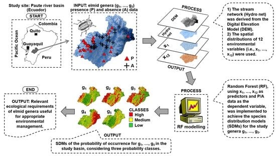
:Simple Summary
Abstract
1. Introduction
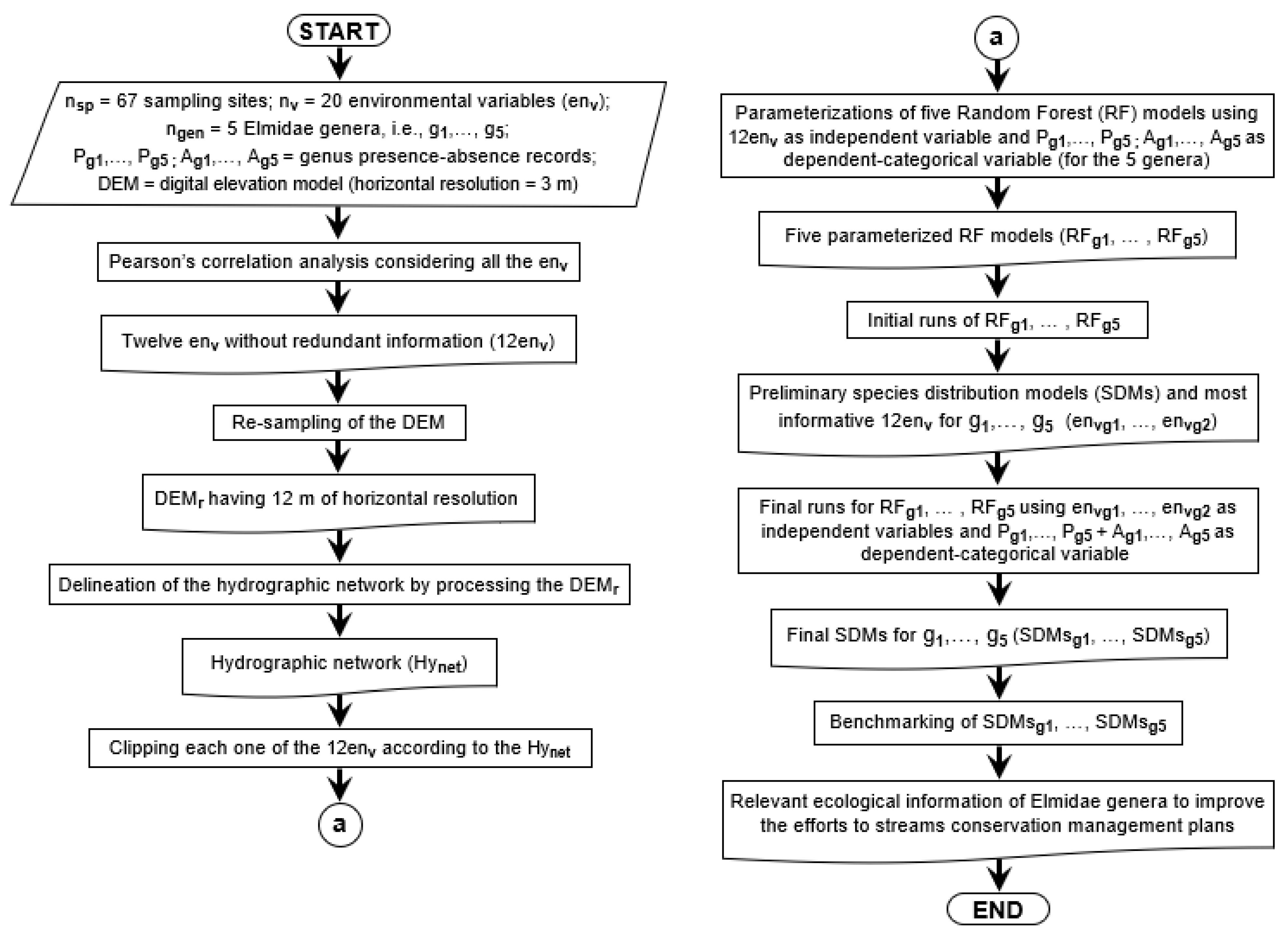
2. Materials and Methods
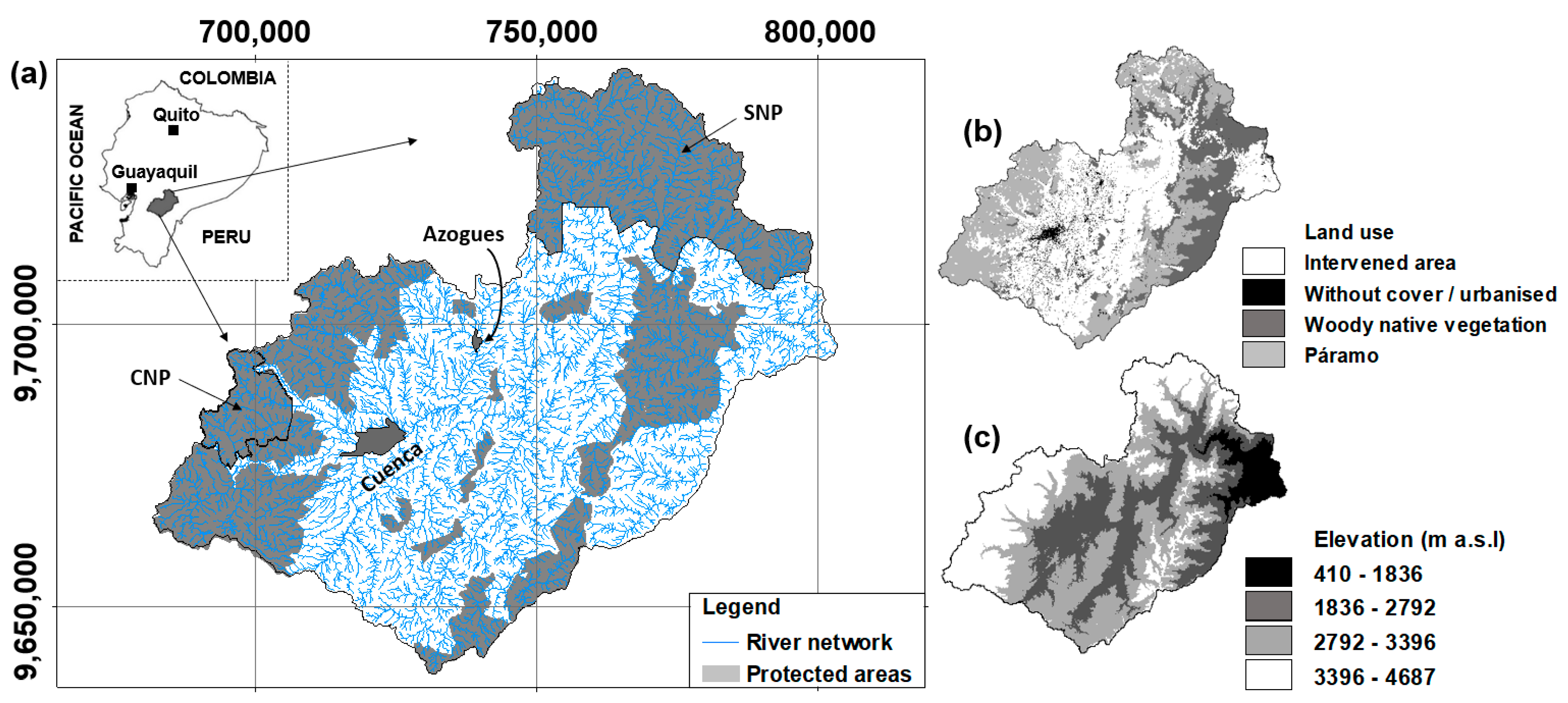
2.1. Study Area
2.2. Sampling of Riffle Beetles
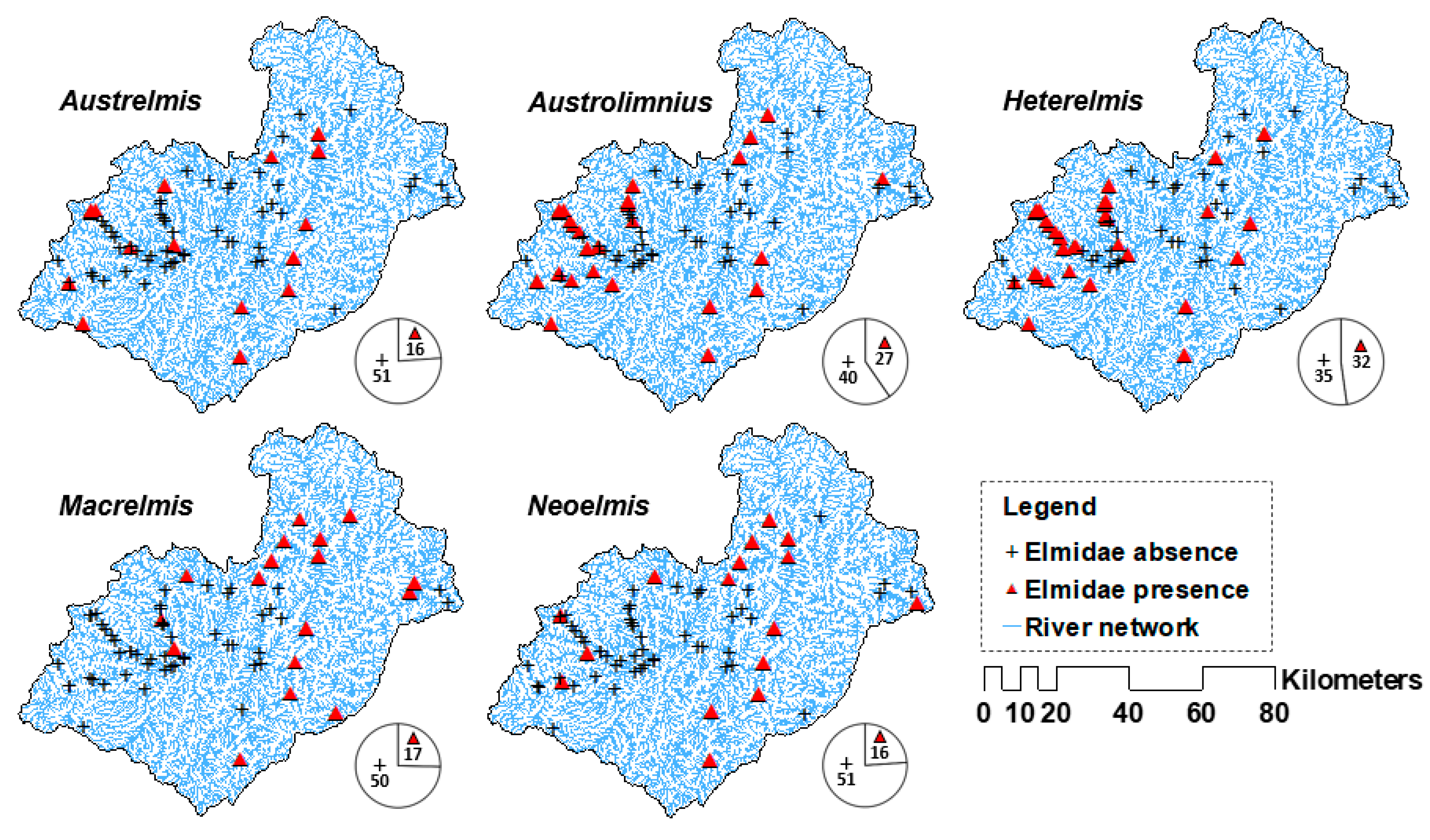
Riffle Beetles and Their Presence–Absence Records
2.3. Environmental Variables
2.4. Species Distribution Models (SDMs) Using Random Forest (RF) Algorithm
Assessing Significant Environmental Variables
2.5. Prediction of Spatial Distribution
2.6. Congruency of the Predicted Spatial Distribution of the C3 Probability of Occurrence of Elmid Genera
3. Results
3.1. Species Distribution Models (SDMs)
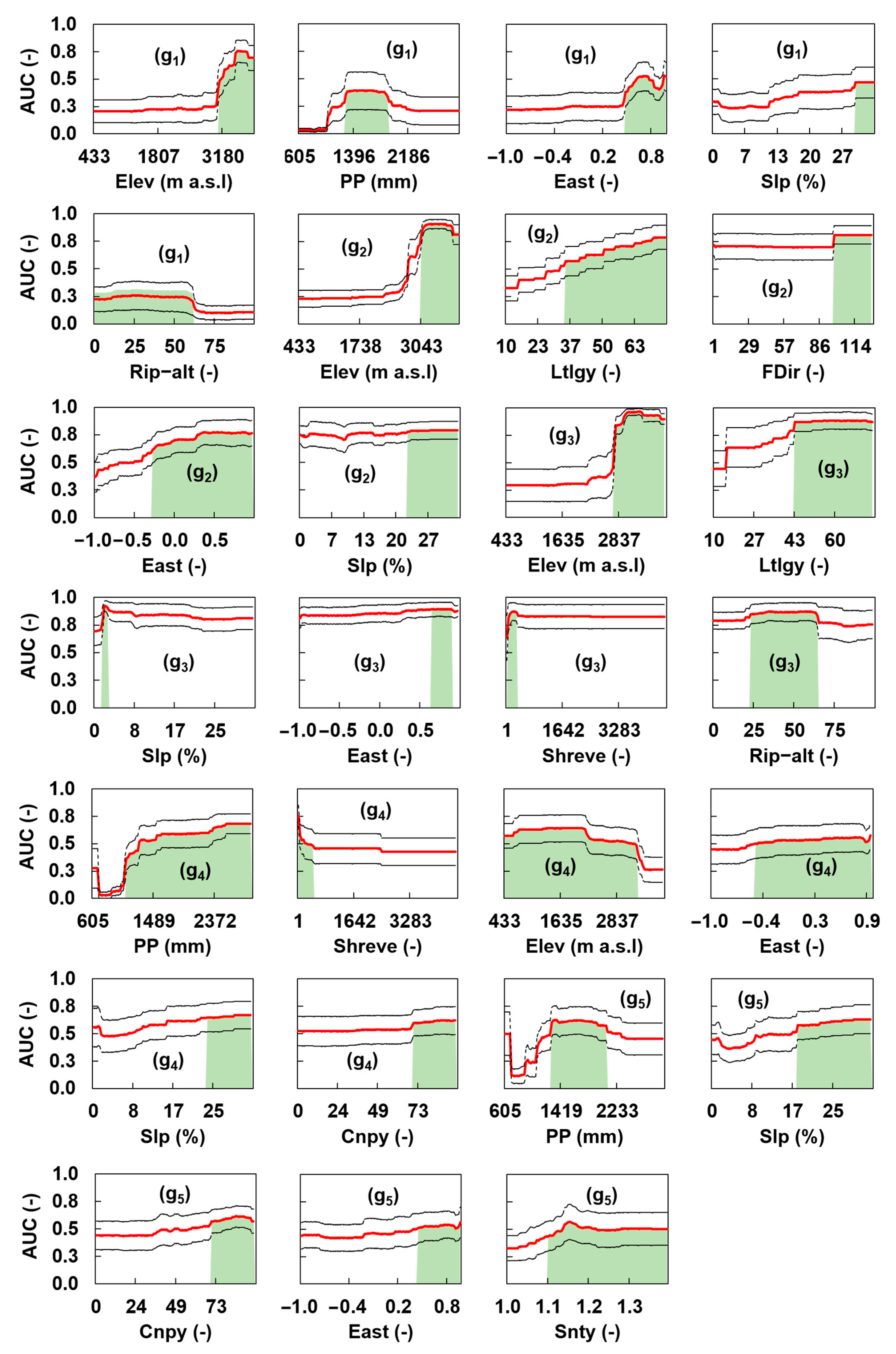
3.2. Assessing Significant Environmental Variables
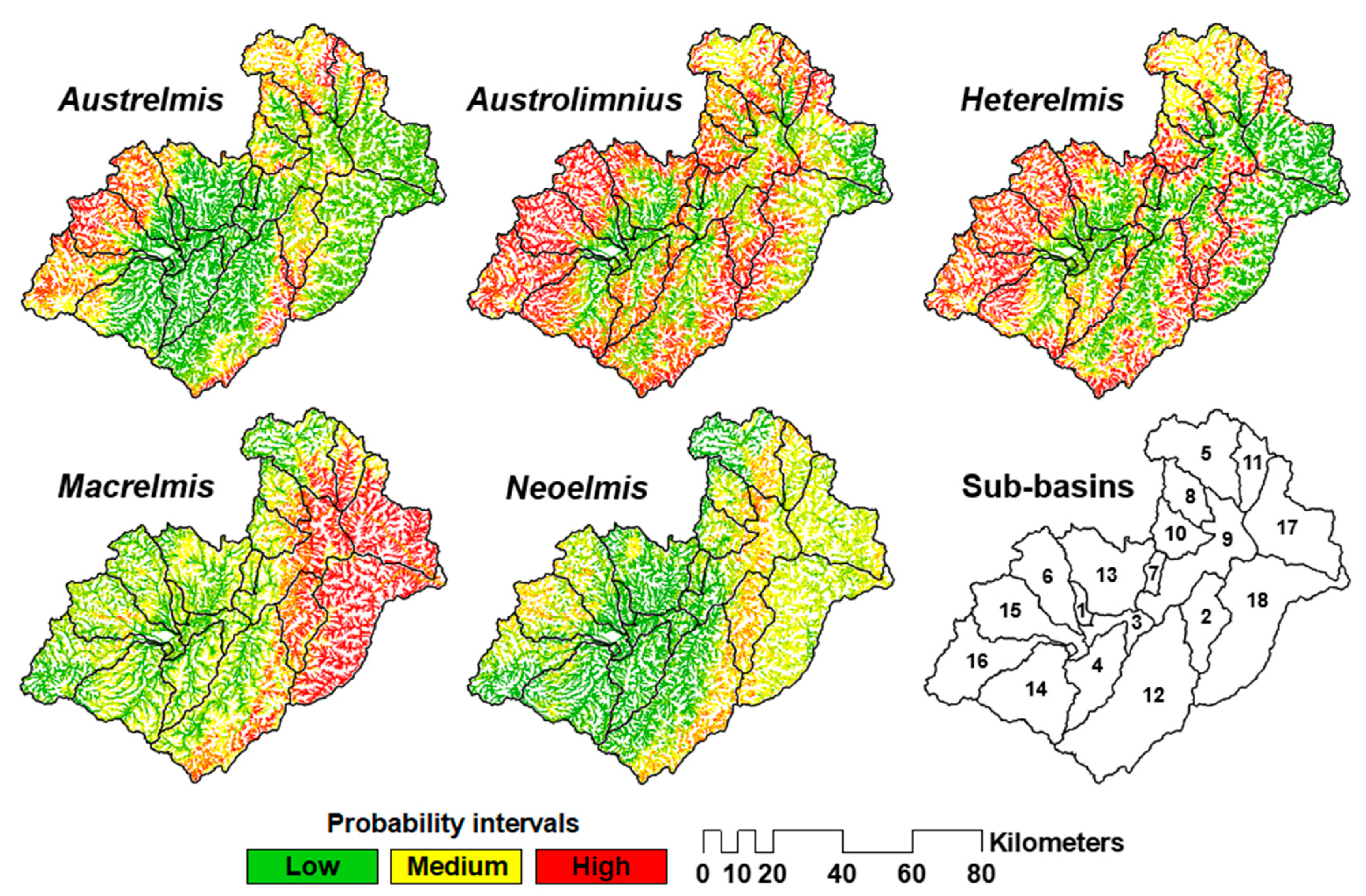
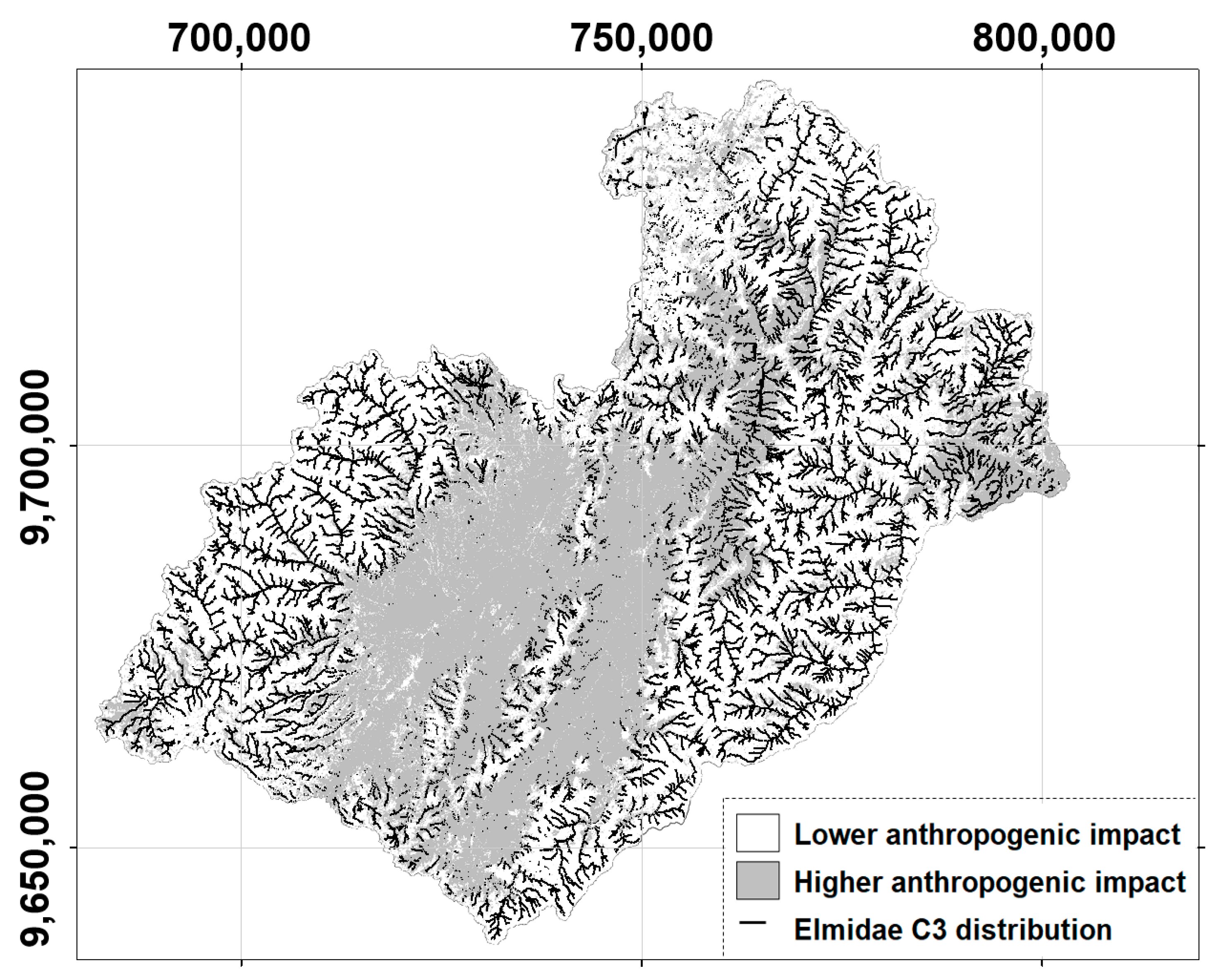
3.3. C3 Class of Occurrence Probability of Elmidae across the Paute River Basin
4. Discussion
4.1. Model Selection
4.2. Model Performance
4.3. Basic Findings of the Developed SDMs
4.4. Important Predictors for Elmids Distribution
4.5. Elmidae Genera’s SDMs and Their Implications for the Surface Water Quality Management in the Study Basin
5. Conclusions
Author Contributions
Funding
Institutional Review Board Statement
Informed Consent Statement
Data Availability Statement
Acknowledgments
Conflicts of Interest
References
- Schmeller, D.S.; Loyau, A.; Bao, K.; Brack, W.; Chatzinotas, A.; De Vleeschouwer, F.; Friesen, J.; Gandois, L.; Hansson, S.V.; Haver, M.; et al. People, pollution and pathogens—Global change impacts in mountain freshwater ecosystems. Sci. Total Environ. 2018, 622–623, 756–763. [Google Scholar] [CrossRef] [Green Version]
- Albert, J.S.; Destouni, G.; Duke-Sylvester, S.M.; Magurran, A.E.; Oberdorff, T.; Reis, R.E.; Winemiller, K.O.; Ripple, W.J. Scientists’ warning to humanity on the freshwater biodiversity crisis. Ambio 2021, 50, 85–94. [Google Scholar] [CrossRef]
- Cañedo-Argüelles, M.; Hermoso, V.; Herrera-Grao, T.; Barquín, J.; Bonada, N. Freshwater conservation planning informed and validated by public participation: The Ebro catchment, Spain, as a case study. Aquat. Conserv. Mar. Freshw. Ecosyst. 2019, 29, 1253–1267. [Google Scholar] [CrossRef]
- Van Echelpoel, W.; Boets, P.; Landuyt, D.; Gobeyn, S.; Everaert, G.; Bennetsen, E.; Mouton, A.; Goethals, P.L. Species distribution models for sustainable ecosystem management. In Developments in Environmental Modelling; Elsevier B.V.: Amsterdam, The Netherlands, 2015; Volume 27. [Google Scholar]
- Zurell, D.; Franklin, J.; König, C.; Bouchet, P.J.; Dormann, C.F.; Elith, J.; Fandos, G.; Feng, X.; Guillera-Arroita, G.; Guisan, A. A standard protocol for reporting species distribution models. Ecography 2020, 43, 1261–1277. [Google Scholar] [CrossRef]
- Besacier Monbertrand, A.L.; Timoner, P.; Rahman, K.; Burlando, P.; Fatichi, S.; Gonseth, Y.; Moser, F.; Castella, E.; Lehmann, A. Assessing the vulnerability of aquatic macroinvertebrates to climatewarming in a mountainouswatershed: Supplementing presence-only data with species traits. Water 2019, 11, 636. [Google Scholar] [CrossRef] [Green Version]
- Mehler, K.; Burlakova, L.E.; Karatayev, A.Y.; Biesinger, Z.; Bruestle, E.; Valle-Levinson, A.; Castiglione, C.; Gorsky, D. Integrating remote sensing and species distribution modelling to predict benthic communities in a Great Lakes connecting channel. River Res. Appl. 2017, 33, 1336–1344. [Google Scholar] [CrossRef]
- Kusch, J. Interacting influences of climate factors and land cover types on the distribution of caddisflies (Trichoptera) in streams of a central European low mountain range. Insect Conserv. Divers. 2015, 8, 92–101. [Google Scholar] [CrossRef]
- Chucholl, C. Niche-based species distribution models and conservation planning for endangered freshwater crayfish in south-western Germany. Aquat. Conserv. Mar. Freshw. Ecosyst. 2017, 27, 698–705. [Google Scholar] [CrossRef]
- Azzurro, E.; Soto, S.; Garofalo, G.; Maynou, F. Fistularia commersonii in the Mediterranean Sea: Invasion history and distribution modeling based on presence-only records. Biol. Invasions 2013, 15, 977–990. [Google Scholar] [CrossRef] [Green Version]
- Rocha, J.C.; Peres, C.K.; Buzzo, J.L.; de Souza, V.; Krause, E.A.; Bispo, P.C.; Frei, F.; Costa, L.S.; Branco, C.C. Modeling the species richness and abundance of lotic macroalgae based on habitat characteristics by artificial neural networks: A potentially useful tool for stream biomonitoring programs. J. Appl. Phycol. 2017, 29, 2145–2153. [Google Scholar] [CrossRef] [Green Version]
- Deknock, A.; De Troyer, N.; Houbraken, M.; Dominguez-Granda, L.; Nolivos, I.; Van Echelpoel, W.; Forio, M.A.; Spanoghe, P.; Goethals, P. Distribution of agricultural pesticides in the freshwater environment of the Guayas river basin (Ecuador). Sci. Total Environ. 2019, 646, 996–1008. [Google Scholar] [CrossRef] [Green Version]
- Celi, J.E.; Villamarín, F. Freshwater ecosystems of mainland Ecuador: Diversity, issues and perspectives. Acta Limnol. Bras. 2020, 32, 1–8. [Google Scholar] [CrossRef]
- Gobeyn, S.; Volk, M.; Dominguez-Granda, L.; Goethals, P.L.M. Input variable selection with a simple genetic algorithm for conceptual species distribution models: A case study of river pollution in Ecuador. Environ. Model. Softw. 2017, 92, 269–316. [Google Scholar] [CrossRef]
- Brown, H. Biology Of Riffle Beetles. Annu. Rev. Entomol. 1987, 32, 253–273. [Google Scholar] [CrossRef]
- Miserendino, M.L.; Archangelsky, M. Aquatic coleoptera distribution and environmental relationships in a large Patagonian river. Int. Rev. Hydrobiol. 2006, 91, 423–437. [Google Scholar] [CrossRef]
- Dos Santos, D.A.; Molineri, C.; Reynaga, M.C.; Basualdo, C. Which index is the best to assess stream health? Ecol. Indic. 2011, 11, 582–589. [Google Scholar] [CrossRef]
- Elliott, J.M. The Ecology of Riffle Beetles (Coleoptera: Elmidae). Freshw. Rev. 2008, 1, 189–203. [Google Scholar] [CrossRef]
- Salazar, G.; Rudnick, H. Hydro power plants in Ecuador: A technical and economical analysis. In Proceedings of the 2008 IEEE Power and Energy Society General Meeting—Conversion and Delivery of Electrical Energy in the 21st Century, Pittsburgh, PA, USA, 20–24 July 2008; pp. 1–5. [Google Scholar] [CrossRef]
- Castillo, L.G.; Álvarez, M.A.; Carrillo, J.M. Numerical modeling of sedimentation and flushing at the Paute-Cardenillo Reservoir. In Proceedings of the ASCE-EWRI International Perspective on Water Resources and Environment, Quito, Ecuador, 8–10 January 2014; pp. 2–11. [Google Scholar]
- Sotomayor, G.; Henrietta, H.; Vázquez, R.F.; Goethals, P.L.M. Multivariate-statistics based selection of a benthic macroinvertebrate index for assessing water quality in the Paute river basin (Ecuador). Ecol. Indic. 2020, 111, 106037. [Google Scholar] [CrossRef] [Green Version]
- González-Córdoba, M.; Del Carmen Zúñiga, M.; Manzo, V. The Elmidae family (Insecta: Coleoptera: Byrrhoidea) in Colombia: Taxonomic richness and distribution. Rev. la Acad. Colomb. Ciencias Exactas Fis. y Nat. 2020, 44, 522–553. [Google Scholar] [CrossRef]
- Legendre, P.; Legendre, L. Numerical Ecology; Elsevier Science B.V.: Amsterdam, The Netherlands, 2012. [Google Scholar]
- Domisch, S.; Jähnig, S.C.; Simaika, J.P.; Kuemmerlen, M.; Stoll, S. Application of species distribution models in stream ecosystems: The challenges of spatial and temporal scale, environmental predictors and species occurrence data. Fundam. Appl. Limnol. 2015, 186, 45–61. [Google Scholar] [CrossRef]
- Jaynes, E.T. Information Theory and Statistical Mechanics. II. Phys. Rev. 1957, 108, 171–190. [Google Scholar] [CrossRef]
- Jaynes, E.T. Information theory and statistical mechanics. Phys. Rev. 1957, 106, 620–630. [Google Scholar] [CrossRef]
- Phillips, S.J.; Dudık, M.; Schapire, R.E. A Maximum Entropy Approach to Species Distribution Modeling. In Proceedings of the Twenty-First International Conference on Machine Learning, Banff, AB, Canada, 4–8 July 2004. [Google Scholar] [CrossRef]
- Johnson, R.A.; Chawla, N.V.; Hellmann, J.J. Species distribution modeling and prediction: A class imbalance problem. In Proceedings of the 2012 Conference on Intelligent Data Understanding, CIDU 2012, Boulder, CO, USA, 24–26 October 2012; pp. 9–16. [Google Scholar] [CrossRef] [Green Version]
- Mi, C.; Huettmann, F.; Guo, Y.; Han, X.; Wen, L. Why choose Random Forest to predict rare species distribution with few samples in large undersampled areas? Three Asian crane species models provide supporting evidence. PeerJ 2017, 5, e2849. [Google Scholar] [CrossRef] [PubMed] [Green Version]
- Fukuda, S.; De Baets, B.; Waegeman, W.; Verwaeren, J.; Mouton, A.M. Habitat prediction and knowledge extraction for spawning European grayling (Thymallus thymallus L.) using a broad range of species distribution models. Environ. Model. Softw. 2013, 47, 1–6. [Google Scholar] [CrossRef]
- Piri Sahragard, H.; Ajorlo, M.; Karami, P. Modeling habitat suitability of range plant species using random forest method in arid mountainous rangelands. J. Mt. Sci. 2018, 15, 2159–2171. [Google Scholar] [CrossRef]
- Cha, Y.; Shin, J.; Go, B.; Lee, D.S.; Kim, Y.; Kim, T.; Park, Y.S. An interpretable machine learning method for supporting ecosystem management: Application to species distribution models of freshwater macroinvertebrates. J. Environ. Manag. 2021, 291, 112719. [Google Scholar] [CrossRef]
- Celleri, R.; Willems, P.; Buytaert, W.; Feyen, J. Space–time rainfall variability in the Paute Basin, Ecuadorian Andes. Hydrol. Process. Int. J. 2007, 21, 3316–3327. [Google Scholar] [CrossRef]
- Sotomayor, G. Evaluación de la Calidad de las Aguas Superficiales Mediante Técnicas de Estadística Multivariante: Un Estudio de Caso en la Cuenca del Río Paute, al Sur de Ecuador. Master’s Thesis, Universidad Nacional de La Plata, La Plata, Argentina, 2016. [Google Scholar]
- Sotomayor, G.; Hampel, H.; Vázquez, R.F. Water quality assessment with emphasis in parameter optimisation using pattern recognition methods and genetic algorithm. Water Res. 2018, 130, 353–362. [Google Scholar] [CrossRef]
- Jacobsen, D.; Schultz, R.; Encalada, A. Structure and diversity of stream invertebrate assemblages: The influence of temperature with altitude and latitude. Freshw. Biol. 1997, 38, 247–261. [Google Scholar] [CrossRef] [Green Version]
- Segura, M.O.; Da Silva Dos Passos, M.I.; Fonseca-Gessner, A.A.; Froehlich, C.G. Elmidae curtis, 1830 (coleoptera, polyphaga, byrrhoidea) of the neotropical region. Zootaxa 2013, 3731, 1–57. [Google Scholar] [CrossRef] [Green Version]
- Curiel, J.; Morrone, J.J. Association of larvae and adults of Mexican species of Macrelmis (Coleoptera: Elmidae): A preliminary analysis using DNA sequences. Zootaxa 2012, 3361, 56–62. [Google Scholar] [CrossRef]
- Cao, Y.; DeWalt, R.E.; Robinson, J.L.; Tweddale, T.; Hinz, L.; Pessino, M. Using Maxent to model the historic distributions of stonefly species in Illinois streams: The effects of regularization and threshold selections. Ecol. Modell. 2013, 259, 30–39. [Google Scholar] [CrossRef]
- Shen, C.; Shi, Y.; Fan, K.; He, J.S.; Adams, J.M.; Ge, Y.; Chu, H. Soil pH dominates elevational diversity pattern for bacteria in high elevation alkaline soils on the Tibetan Plateau. FEMS Microbiol. Ecol. 2019, 95, fiz003. [Google Scholar] [CrossRef] [PubMed] [Green Version]
- Warren, D.L.; Matzke, N.J.; Cardillo, M.; Baumgartner, J.B.; Beaumont, L.J.; Turelli, M.; Glor, R.E.; Huron, N.A.; Simões, M.; Iglesias, T.L.; et al. ENMTools 1.0: An R package for comparative ecological biogeography. Ecography 2021, 44, 504–511. [Google Scholar] [CrossRef]
- Corral, L.R.; Montiel Olea, C.E. What Drives Take-up in Land Regularization: Ecuador’s Rural Land Regularization and Administration Program, Sigtierras. J. Econ. Race Policy 2020, 3, 60–75. [Google Scholar] [CrossRef]
- McCoy, J.; Johnston, K.; Kopp, S.; Borup, B.; Willison, J.; Payne, B. Using ArcGIS™ Spatial Analyst, GIS by ESRI. Redlands, California: Environmental Systems Research Institute Inc. 2002. Available online: http://downloads.esri.com/support/documentation/ao_/776Using_Spatial_Analyst.pdf (accessed on 7 February 2022).
- Arif, F.; Akbar, M. Resampling air borne sensed data using bilinear interpolation algorithm. In Proceedings of the IEEE International Conference on Mechatronics, 2005, ICM ′05, Taipei, Taiwan, 10–12 July 2005; Volume 2005, pp. 62–65. [Google Scholar]
- Bajjali, W. ArcGIS for Environmental and Water Issues; Springer Textbooks in Earth Sciences, Geography and Environment; Springer: Berlin/Heidelberg, Germany, 2018. [Google Scholar] [CrossRef]
- Tarboton, D.G.; Bras, R.L.; Rodriguez-Iturbe, I. On the extraction of channel networks from digital elevation data. Hydrol. Process. 1991, 5, 81–100. [Google Scholar] [CrossRef]
- Vázquez, R.F.; Feyen, J. Assessment of the effects of DEM gridding on the predictions of basin runoff using MIKE SHE and a modelling resolution of 600 m. J. Hydrol. 2007, 334, 73–87. [Google Scholar] [CrossRef]
- Li, Y.; Lei, N.; Xiong, Y. Research on Watershed Extraction Method Based on GIS. IOP Conf. Ser. Earth Environ. Sci. 2019, 300, 022168. [Google Scholar] [CrossRef]
- Kuemmerlen, M.; Schmalz, B.; Guse, B.; Cai, Q.; Fohrer, N.; Jähnig, S.C. Integrating catchment properties in small scale species distribution models of stream macroinvertebrates. Ecol. Modell. 2014, 277, 77–86. [Google Scholar] [CrossRef]
- Jacobsen, D. Altitudinal changes in diversity of macroinvertebrates from small streams in the Ecuadorian Andes. Arch. Hydrobiol. 2003, 158, 145–167. [Google Scholar] [CrossRef]
- Jacobsen, D. Contrasting patterns in local and zonal family richness of stream invertebrates along an Andean altitudinal gradient. Freshw. Biol. 2004, 49, 1293–1305. [Google Scholar] [CrossRef]
- Braun, B.M.; Salvarrey, A.V.B.; Kotzian, C.B.; Spies, M.R.; Pires, M.M. Diversity and distribution of riffle beetle assemblages (Coleoptera, Elmidae) in montane rivers of Southern Brazil. Biota Neotrop. 2014, 14, 2. [Google Scholar] [CrossRef] [Green Version]
- Harrison, E.T.; Norris, R.; Wilkinson, S.N. The impact of fine sediment accumulation on benthic macroinvertebrates: Implications for river management. In Proceedings of the 5th Australian Stream Management Conference: Australian Rivers: Making a Difference, Albury, NSW, Australia, 21–25 May 2007; pp. 139–144. [Google Scholar]
- Miserendino, M.L. Macroinvertebrate assemblages in Andean Patagonian rivers and streams: Environmental relationships. Hydrobiologia 2001, 444, 147–158. [Google Scholar] [CrossRef]
- Roberts, D.W. Ordination on the basis of fuzzy set theory. Vegetatio 1986, 66, 123–131. [Google Scholar] [CrossRef]
- Eichenberg, D.; Pietsch, K.; Meister, C.; Ding, W.; Yu, M.; Wirth, C. The effect of microclimate on wood decay is indirectly altered by tree species diversity in a litterbag study. J. Plant Ecol. 2017, 10, 170–178. [Google Scholar] [CrossRef] [Green Version]
- Vannucchi, P.E.; López-Rodríguez, M.J.; Tierno de Figueroa, J.M.; Gaino, E. Structure and dynamics of a benthic trophic web in a Mediterranean seasonal stream. J. Limnol. 2013, 72, 606–615. [Google Scholar] [CrossRef]
- Dilts, T.; Yang, J. Stream Gradient and Sinuosity Toolbox for ArcGIS 10.1; University of Nevada: Las Vegas, NV, USA, 2015. [Google Scholar]
- Ferreira, W.R.; Ligeiro, R.; Macedo, D.R.; Hughes, R.M.; Kaufmann, P.R.; Oliveira, L.G.; Callisto, M. Importance of environmental factors for the richness and distribution of benthic macroinvertebrates in tropical headwater streams. Freshw. Sci. 2014, 33, 860–871. [Google Scholar] [CrossRef]
- Braun, B.M.; Kotzian, C.B.; Gonçalves, A.S.; Pires, M.M. Potential distribution of riffle beetles (Coleoptera: Elmidae) in southern Brazil. Austral Entomol. 2018, 58, 646–665. [Google Scholar] [CrossRef]
- Smith, J.V. Colloquium on Geology, Mineralogy, and Human Welfare; National Academies Press: Washington, DC, USA, 1999; Volume 96. [Google Scholar]
- Wolmarans, C.T.; Kemp, M.; de Kock, K.N.; Wepener, V. The possible association between selected sediment characteristics and the occurrence of benthic macroinvertebrates in a minimally affected river in South Africa. Chem. Ecol. 2017, 33, 18–33. [Google Scholar] [CrossRef]
- Battle, J.; Golladay, S.W. Water quality and macroinvertebrate assemblages in three types of seasonally inundated limesink wetlands in southwest Georgia. J. Freshw. Ecol. 2001, 16, 189–207. [Google Scholar] [CrossRef] [Green Version]
- Endries, M. Aquatic Species Mapping in North Carolina Using Maxent; US Fish and Wildlife Service, Ecological Services Field Office: Lakewood, CO, USA, 2011.
- Tchoukanski, I. Create Non-Overlapping Buffers with Attributes. 2021. Available online: https://www.ian-ko.com/ET_SolutionCenter/gw_create_non_overlapping_buffers.htm (accessed on 16 May 2022).
- Forio, M.A.; Burdon, F.J.; De Troyer, N.; Lock, K.; Witing, F.; Baert, L.; De Saeyer, N.; Rîșnoveanu, G.; Popescu, C.; Kupilas, B. A Bayesian Belief Network learning tool integrates multi-scale effects of riparian buffers on stream invertebrates. Sci. Total Environ. 2022, 810, 152146. [Google Scholar] [CrossRef] [PubMed]
- Beschta, R.L. Riparian shade and stream temperature: An alternative perspective. Rangelands 1997, 19, 25–28. [Google Scholar]
- Amatulli, G.; McInerney, D.; Sethi, T.; Strobl, P.; Domisch, S. Geomorpho90m, empirical evaluation and accuracy assessment of global high-resolution geomorphometric layers. Sci. Data 2020, 7, 162. [Google Scholar] [CrossRef] [PubMed]
- Breiman, L. Random forests. Mach. Learn. 2001, 45, 5–32. [Google Scholar] [CrossRef] [Green Version]
- Valavi, R.; Elith, J.; Lahoz-Monfort, J.J.; Guillera-Arroita, G. Modelling species presence-only data with random forests. Ecography 2021, 44, 1731–1742. [Google Scholar] [CrossRef]
- Thuiller, W.; Georges, D.; Gueguen, M.; Engler, R.; Breiner, F. biomod2: Ensemble Platform for Species Distribution Modeling. R Package Version 3.5.1.; R Team: Vienna, Austria, 2021. [Google Scholar]
- Fox, E.W.; Hill, R.A.; Leibowitz, S.G.; Olsen, A.R.; Thornbrugh, D.J.; Weber, M.H. Assessing the accuracy and stability of variable selection methods for random forest modeling in ecology. Environ. Monit. Assess. 2017, 189, 316. [Google Scholar] [CrossRef]
- Probst, P.; Wright, M.N.; Boulesteix, A.L. Hyperparameters and tuning strategies for random forest. Wiley Interdiscip. Rev. Data Min. Knowl. Discov. 2019, 9, e1301. [Google Scholar] [CrossRef] [Green Version]
- Strobl, C.; Boulesteix, A.L.; Zeileis, A.; Hothorn, T. Bias in random forest variable importance measures: Illustrations, sources and a solution. BMC Bioinform. 2007, 8, 25. [Google Scholar] [CrossRef] [Green Version]
- Strobl, C.; Boulesteix, A.L.; Kneib, T.; Augustin, T.; Zeileis, A. Conditional variable importance for random forests. BMC Bioinform. 2008, 9, 307. [Google Scholar] [CrossRef] [Green Version]
- Xiong, Z.; Cui, Y.; Liu, Z.; Zhao, Y.; Hu, M.; Hu, J. Evaluating explorative prediction power of machine learning algorithms for materials discovery using k-fold forward cross-validation. Comput. Mater. Sci. 2020, 171, 109203. [Google Scholar] [CrossRef]
- Grimm, K.J.; Mazza, G.L.; Davoudzadeh, P. Model Selection in Finite Mixture Models: A k-Fold Cross-Validation Approach. Struct. Equ. Model. 2017, 24, 246–256. [Google Scholar] [CrossRef]
- Pal, K.; Patel, B.V. Data Classification with k-fold Cross Validation and Holdout Accuracy Estimation Methods with 5 Different Machine Learning Techniques. In Proceedings of the 2020 Fourth International Conference on Computing Methodologies and Communication (ICCMC), Erode, India, 11–13 March 2020; pp. 83–87. [Google Scholar] [CrossRef]
- Khalilia, M.; Chakraborty, S.; Popescu, M. Predicting disease risks from highly imbalanced data using random forest. BMC Med. Inform. Decis. Mak. 2011, 11, 51. [Google Scholar] [CrossRef] [PubMed] [Green Version]
- Brown, I.; Mues, C. An experimental comparison of classification algorithms for imbalanced credit scoring data sets. Expert Syst. Appl. 2012, 39, 3446–3453. [Google Scholar] [CrossRef] [Green Version]
- Larras, F.; Coulaud, R.; Gautreau, E.; Billoir, E.; Rosebery, J.; Usseglio-Polatera, P. Assessing anthropogenic pressures on streams: A random forest approach based on benthic diatom communities. Sci. Total Environ. 2017, 586, 1101–1112. [Google Scholar] [CrossRef]
- Boulesteix, A.L.; Janitza, S.; Kruppa, J.; König, I.R. Overview of random forest methodology and practical guidance with emphasis on computational biology and bioinformatics. Wiley Interdiscip. Rev. Data Min. Knowl. Discov. 2012, 2, 493–507. [Google Scholar] [CrossRef] [Green Version]
- Rebala, G.; Ravi, A.; Churiwala, S. Random forests. In An Introduction to Machine Learning; Springer Nature: Cham, Switzerland, 2019; pp. 77–94. [Google Scholar] [CrossRef] [Green Version]
- Ballabio, D.; Grisoni, F.; Todeschini, R. Multivariate comparison of classification performance measures. Chemom. Intell. Lab. Syst. 2018, 174, 33–44. [Google Scholar] [CrossRef]
- Sokolova, M.; Japkowicz, N.; Szpakowicz, S. Beyond Accuracy, F-Score and ROC: A Family of Discriminant Measures for Performance Evaluation. In AI 2006: Advances in Artificial Intelligence; Carbonell, J.G., Siekmann, J., Eds.; Springer: Berlin/Heidelberg, Germany, 2006; pp. 1015–1021. [Google Scholar] [CrossRef] [Green Version]
- Sotomayor, G.; Hampel, H.; Vázquez, R.F.; Forio, M.A.E.; Goethals, P.L.M. Implications of macroinvertebrate taxonomic resolution for freshwater assessments using functional traits: The Paute River Basin (Ecuador) case. Divers. Distrib. 2021, 28, 1735–1747. [Google Scholar] [CrossRef]
- Shapiro, S.S.; Wilk, M.B. An Analysis of Variance Test for Normality (Complete Samples). Biometrika Trust 1965, 52, 591–611. [Google Scholar] [CrossRef]
- Anderson, T.; Finn, J. The New Statistical Analysis of Data; Springer: New York, NY, USA, 1996. [Google Scholar]
- Helsel, D.R.; Hirsch, R.M.; Ryberg, K.R.; Archfield, S.A.; Gilroy, E. Statistical Methods in Water Resources. In Book 4, Hydrologic Analysis and Interpretation; U.S. Geological Survey: Washington, DC, USA, 2020; p. 458. [Google Scholar]
- Hosmer, D.W., Jr.; Lemeshow, S.; Sturdivant, R.X. Applied Logistic Regression; John Wiley & Sons, Inc.: Hoboken, NJ, USA, 2013; Volume 38. [Google Scholar]
- Thuiller, W.; Lafourcade, B.; Engler, R.; Araújo, M.B. BIOMOD—A platform for ensemble forecasting of species distributions. Ecography 2009, 32, 369–373. [Google Scholar] [CrossRef]
- Jain, A.K. Data clustering: 50 years beyond K-means. Pattern Recognit. Lett. 2010, 31, 651–666. [Google Scholar] [CrossRef]
- Hammer, Ø. PAST: Paleontological Statistics Version 4.03—Reference Manual; Natural History Museum University of Oslo: Oslo, Norway, 2020; pp. 1–283. [Google Scholar]
- Wang, K.; Wang, B.; Peng, L. CVAP: Validation for Cluster Analyses. Data Sci. J. 2009, 8, 88–93. [Google Scholar] [CrossRef]
- Thalamuthu, A.; Mukhopadhyay, I.; Zheng, X.; Tseng, G. Evaluation and comparison of gene clustering methods in microarray analysis. Bioinformatics 2006, 22, 2405–2412. [Google Scholar] [CrossRef] [PubMed] [Green Version]
- Kaufman, L.; Rousseeuw, P.J. Finding Groups in Data—An Introduction to Cluster Analysis; John Wiley & Sons, Inc.: Hoboken, NJ, USA, 1990. [Google Scholar]
- Guisan, A.; Thuiller, W.; Zimmermann, N.E. Habitat Suitability and Distribution Models: With Applications in R; Cambridge University Press: Cambridge, UK, 2017. [Google Scholar] [CrossRef]
- Ministerio del Ambiente del Ecuador (MAE). Sistema de Clasificación de Ecosistemas del Ecuador Continental; Subsecretaría de Patrimonio Natural—Proyecto Mapa de Vegetación: Quito, Ecuador, 2013. [Google Scholar]
- Lissovsky, A.A.; Dudov, S.V. Species-Distribution Modeling: Advantages and Limitations of Its Application. 2. MaxEnt. Biol. Bull. Rev. 2021, 11, 265–275. [Google Scholar] [CrossRef]
- Cárdenas, R.E.; Buestán, J.; Dangles, O. Diversity and distribution models of horse flies (diptera: Tabanidae) from ecuador. Ann. La Soc. Entomol. Fr. 2009, 45, 511–528. [Google Scholar] [CrossRef] [Green Version]
- Escobar, L.E.; Romero-Alvarez, D.; Leon, R.; Lepe-Lopez, M.A.; Craft, M.E.; Borbor-Cordova, M.J.; Svenning, J.C. Declining Prevalence of Disease Vectors Under Climate Change. Sci. Rep. 2016, 6, 39150. [Google Scholar] [CrossRef] [Green Version]
- Cuesta, F.; Peralvo, M.; Merino-Viteri, A.; Bustamante, M.; Baquero, F.; Freile, J.F.; Muriel, P.; Torres-Carvajal, O. Priority areas for biodiversity conservation in mainland Ecuador. Neotrop. Biodivers. 2017, 3, 93–106. [Google Scholar] [CrossRef] [Green Version]
- Moya, W.; Jacome, G.; Yoo, C.K. Past, current, and future trends of red spiny lobster based on PCA with MaxEnt model in Galapagos Islands, Ecuador. Ecol. Evol. 2017, 7, 4881–4890. [Google Scholar] [CrossRef] [PubMed]
- Yañez-Arenas, C.; Díaz-Gamboa, L.; Patrón-Rivero, C.; López-Reyes, K.; Chiappa-Carrara, X. Estimating geographic patterns of ophidism risk in Ecuador. Neotrop. Biodivers. 2018, 4, 55–61. [Google Scholar] [CrossRef] [Green Version]
- Jácome, G.; Vilela, P.; Yoo, C.K. Present and future incidence of dengue fever in Ecuador nationwide and coast region scale using species distribution modeling for climate variability’s effect. Ecol. Modell. 2019, 400, 60–72. [Google Scholar] [CrossRef]
- Kübler, D. Effect of Topography on the Distribution of tree Species and Radial Diameter Growth of Potential Crop Trees in a Tropical Mountain Forest in Southern Ecuador. Ph.D. Thesis, Technische Universität München, Munich, Germany, 2020. [Google Scholar]
- Yackulic, C.B.; Chandler, R.; Zipkin, E.F.; Royle, J.A.; Nichols, J.D.; Campbell Grant, E.H.; Veran, S. Presence-only modelling using MAXENT: When can we trust the inferences? Methods Ecol. Evol. 2013, 4, 236–243. [Google Scholar] [CrossRef]
- Ward, G.; Hastie, T.; Barry, S.; Elith, J.; Leathwick, J.R. Presence-Only Data and the EM Algorithm. Biometrics 2009, 65, 554–563. [Google Scholar] [CrossRef] [Green Version]
- Elith, J.; Phillips, S.J.; Hastie, T.; Dudík, M.; Chee, Y.E.; Yates, C.J. A statistical explanation of MaxEnt for ecologists. Divers. Distrib. 2011, 17, 43–57. [Google Scholar] [CrossRef]
- Marmion, M.; Parviainen, M.; Luoto, M.; Heikkinen, R.K.; Thuiller, W. Evaluation of consensus methods in predictive species distribution modelling. Divers. Distrib. 2009, 15, 59–69. [Google Scholar] [CrossRef]
- Drew, C.A.; Wiersma, Y.F.; Huettmann, F. Predictive species and habitat modeling in landscape ecology: Concepts and applications. In Predictive Species and Habitat Modeling in Landscape Ecology: Concepts and Applications; Springer: Berlin/Heidelberg, Germany, 2011; pp. 1–313. [Google Scholar] [CrossRef]
- De Luis, M.; Aálvarez-Jiménez, J.; Rejos, F.J.; Bartolomé, C. Using species distribution models to locate the potential cradles of the allopolyploid Gypsophila bermejoi G. López (Caryophyllaceae). PLoS ONE 2020, 15, e0232736. [Google Scholar] [CrossRef] [PubMed]
- Garcia-Criado, F.; Fernandez-Alaez, M. Hydraenidae and Elmidae assemblages (Coleoptera) from a Spanish river basin: Good indicators of coal mining pollution? Arch. Hydrobiol. 2001, 150, 641–660. [Google Scholar] [CrossRef]
- Von Ellenrieder, N. Composition and structure of aquatic insect assemblages of Yungas mountain cloud forest streams in NW Argentina. Rev. La Soc. Entomol. Argent. 2007, 66, 57–76. [Google Scholar]
- Albanesi, S.A.; Cristobal, L.; Manzo, V.; Nieto, C. Dataset of the baetidae (Ephemeroptera) and elmidae (coleoptera) families from the yungas of Argentina. Rev. La Soc. Entomol. Argent. 2020, 79, 17–23. [Google Scholar] [CrossRef]
- García-Ríos, R.F.; Moi, D.A.; Peláez, O.E. Efectos del gradiente altitudinal sobre las comunidades de macroinvertebrados bentónicos en dos períodos hidrológicos en un río altoandino neotropical. Ecol. Austral 2020, 30, 033–044. [Google Scholar] [CrossRef]
- Monte, C.; Mascagni, A. Review of the Elmidae of Ecuador with the description of ten new species (Coleoptera: Elmidae). Zootaxa 2012, 38, 1–38. [Google Scholar] [CrossRef]
- Linský, M.; Čiamporová-Zaťovičová, Z.; Čiampor, F. Four new species of hexanchorus sharp from Ecuador (Coleoptera, elmidae) with dna barcoding and notes on the distribution of the genus. Zookeys 2019, 2019, 85–109. [Google Scholar] [CrossRef]
- Čiampor, F.; Kodada, J.; Bozáňová, J.; Čiamporová-Zaťovičová, Z. Disersus otongachi a new species of Larainae riffle beetles from Ecuador (Coleoptera: Elmidae). Zootaxa 2021, 4963, 193–199. [Google Scholar] [CrossRef]
- Kattel, D.B.; Yao, T.; Yang, W.; Gao, Y.; Tian, L. Comparison of temperature lapse rates from the northern to the southern slopes of the Himalayas. Int. J. Climatol. 2015, 35, 4431–4443. [Google Scholar] [CrossRef]
- Acosta, R. Estudio de la Cuenca Altoandina del Río Cañete (Perú): Distribución Altitudinal de la Comunidad de Macroinvertebrados Bentónicos y Caracterización Hidroquímica de sus Cabeceras Cársticas. Doctoral Thesis, Universitat de Barcelona, Barcelona, Spain, 2009. [Google Scholar]
- Aguilera Giraldo, I.A.; Vásquez- Ramos, J.M. Distribución espacial y temporal de Elmidae (Insecta: Coleoptera) y su relación con los parámetros fisicoquímicos en el río Ocoa, Meta, Colombia. Rev. La Acad. Colomb. Cienc. Exactas Físicas Nat. 2019, 43, 108. [Google Scholar] [CrossRef]
- Burk, R.A.; Kennedy, J.H. Invertebrate communities of groundwater-dependent refugia with varying hydrology and riparian cover during a supraseasonal drought. J. Freshw. Ecol. 2013, 28, 251–270. [Google Scholar] [CrossRef] [Green Version]
- Pacheco, G.S.M.; Pellegrini, T.G.; Lopes Ferreira, R. Cave lithology influencing EPT (Ephemeroptera, Plecoptera, Trichoptera) assemblages and habitat structure in south-eastern Brazil. Mar. Freshw. Res. 2021, 72, 1546–1552. [Google Scholar] [CrossRef]
- Mora, D.E.; Willems, P. Decadal oscillations in rainfall and air temperature in the Paute River Basin-Southern Andes of Ecuador. Theor. Appl. Climatol. 2012, 108, 267–282. [Google Scholar] [CrossRef] [Green Version]
- Ríos-Touma, B.; Encalada, A.C.; Prat Fornells, N. Macroinvertebrate assemblages of an Andean high-altitude tropical stream: The importance of season and flow. Int. Rev. Hydrobiol. 2011, 96, 667–685. [Google Scholar] [CrossRef]
- Spangler, P.J.; Santiago-Fragoso, S. The Aquatic Beetle Subfamily Larainae (Coleoptera: Elmidae) in Mexico, Central America, and the West Indies; Smithsonian Contributions to Zoology; Smithsonian: Washington, DC, USA, 1992; pp. 1–74. [Google Scholar] [CrossRef]
- Spangler, P.J. Two new species of the aquatic beetle genus Macrelmis Motschulsky from Venezuela (Coleoptera: Elmidae: Elminae). Insecta Mundi 1997, 11, 1–8. [Google Scholar]
- Fernandes, A.S. Taxonomia de Elmidae (Insecta, Coleoptera) do Município de Presidente Figueiredo, Amazonas, Brasil; Instituto Nacional de Pesquisas da Amazônia: Manaus, Brazil, 2010; p. 140. [Google Scholar]
- Braun, B.M.; Pires, M.M.; Stenert, C.; Maltchik, L.; Kotzian, C.B. Effects of riparian vegetation width and substrate type on riffle beetle community structure. Entomol. Sci. 2018, 21, 66–75. [Google Scholar] [CrossRef]
- Brown, A.G.; Rhodes, E.J.; Davis, S.; Zhang, Y.; Pears, B.; Whitehouse, N.J.; Bradley, C.; Bennett, J.; Schwenninger, J.L.; Firth, A.; et al. Late Quaternary evolution of a lowland anastomosing river system: Geological-topographic inheritance, non-uniformity and implications for biodiversity and management. Quat. Sci. Rev. 2021, 260, 106929. [Google Scholar] [CrossRef]
- Da Ros, G. La Contaminación de Aguas en Ecuador: Una Aproximación Económica; Instituto de Investigaciones Económicas, Pontificia Universidad Católica del Ecuador: Quito, Ecuador, 1995. [Google Scholar]
- Pauta Calle, G.; Chang Gómez, J. Indices de calidad del agua de fuentes superficiales y aspectos toxicológicos, evaluación del Río Burgay. Maskana 2014, 5, 165–176. [Google Scholar]


| Source | Variable | Used Tool in ArcGis/ Methodology | Unit | Abbreviation | Ecological Importance | Range | |
|---|---|---|---|---|---|---|---|
| Name | Type | ||||||
| DEM of SIGTIERRAS project (Corral and Montiel Olea, 2020) | Elevation | Continuous | Spatial Analyst > Hydrology > Fill | m a.s.l | Elev | Temperature tends to be colder at higher elevations, e.g., in páramo ecosystems, influencing water dissolved oxygen values [50,51,52]. | 411–4212 |
| Slope | Continuous | Spatial Analyst > Surface > Slope | Degree | Slp | Water velocity and, consequently, oxygen content, are related to slope [21]. | 0–74.1 | |
| Flow direction | Categorical | Spatial Analyst > Hydrology > Flow Direction | (-) | Fdir | Flow direction is related to substrate accumulation and streambed heterogeneity [53]. | 1–128 | |
| Shreve stream order | Continuous | Spatial Analyst > Hydrology > Stream Order | (-) | Shreve | High-stream order values are indicators of bigger discharges [21,54]. | 1–5367 | |
| Eastness | Continuous | Spatial Analyst > Map Algebra > Raster Calculator [55] | (-) | East | These factors are related to the terrain declivity, stream course direction, and luminosity, which affect water temperature, oxygen [56], and algae growth. Algae are food sources for certain elmids [57]. | −1–1 | |
| Northness | Continuous | Ntns | |||||
| Sinuosity | Continuous | Stream Gradient and Sinuosity > Shapefiles > Calculate Sinuosity [58] | (-) | Snty | The sinuosity is related to the accumulation of sediments and channel heterogeneity [59]. | 1–4.8 | |
| National Institute of Meteorology and Hydrology (http://www.inamhi.gob.ec accessed on 7 February 2022) | Precipitation | Continuous | Spatial Analyst > Map Algebra > Raster Calculator | mm | PP | Precipitation is directly related to water availability and indirectly to water velocity and oxygen content [60]. | 586.5–3237.7 |
| Geopedological map, scale 1:25,000; SIGTIERRAS project (Corral and Montiel Olea, 2020) | Lithology | Categorical | Conversion > To Raster > Polygon to Raster | (-) | Ltlgy | Elements in the water and sediments of rivers are present because of the natural weathering of the surrounding lithology [61]. These elements conditionate the elmids [62]. | 1–78 |
| Soil type | Categorical | Conversion > To Raster > Polygon to Raster | (-) | Soils | Water chemistry of rivers is affected by surrounding soil units [63]. | 1–10 | |
| Land Use map, scale 1:100,000 (MAE, 2013) | Riparian alteration | Continuous | [64,65] | % | Rip-alt | The riparian zones regulate water temperature and allochthonous organic matter inputs and mitigate the effects of anthropogenic pressures [21,66]. | 0–99 |
| Global Land Analysis and Discover (https://glad.umd.edu/dataset/ge accessed on 7 February 2022) | Canopy | Continuous | Data Management > Raster > Raster Processing > Resample | (-) | Cnpy | Canopy attenuates the sunlight, regulates the water temperature of streams and favours streambed heterogeneity [66,67]. | 0–100 |
| AUC | SDM of Probability of Occurrence | |||||
|---|---|---|---|---|---|---|
| Genus | Mean/Median | Probability Range | Spatial Extent (%) | |||
| (Step 1) | (Step 2) | C1 | C2 | C3 | ||
| Austrelmis | 0.76 | 0.83 | 0.00–0.94 | 52.8 | 35.4 | 11.9 |
| Austrolimnius | 0.87 | 0.89 * | 0.00–1.00 | 25.0 | 37.4 | 37.7 |
| Heterelmis | 0.76 | 0.79 | 0.01–0.99 | 33.3 | 34.9 | 31.7 |
| Macrelmis | 0.76 | 0.82 | 0.00–0.94 | 28.6 | 41.4 | 30.0 |
| Neoelmis | 0.70 | 0.76 | 0.00–0.87 | 48.1 | 48.9 | 2.9 |
| Genera | Environmental Variable and Its Weight (%) | |||||
|---|---|---|---|---|---|---|
| Austrelmis | Elev * | PP * | East * | Slp * | Rip-alt * | |
| 28.92 | 24.56 | 16.90 | 6.45 | 5.57 | ||
| Austrolimnius | Elev | Ltlgy * | East * | Fdir * | Slp * | |
| 51.70 | 35.39 | 4.10 | 2.11 | 1.86 | ||
| Heterelmis | Elev | Ltlgy | Slp * | East | Shreve * | Rip-alt * |
| 52.27 | 26.95 | 6.63 | 5.00 | 3.27 | 2.06 | |
| Macrelmis | PP | Shreve | Elev * | East | Slp * | Cnpy * |
| 53.56 | 19.56 | 7.17 | 6.23 | 5.76 | 2.83 | |
| Neoelmis | PP | Slp | Cnpy | East * | Snty | |
| 47.62 | 10.06 | 9.41 | 6.38 | 5.45 | ||
Disclaimer/Publisher’s Note: The statements, opinions and data contained in all publications are solely those of the individual author(s) and contributor(s) and not of MDPI and/or the editor(s). MDPI and/or the editor(s) disclaim responsibility for any injury to people or property resulting from any ideas, methods, instructions or products referred to in the content. |
© 2023 by the authors. Licensee MDPI, Basel, Switzerland. This article is an open access article distributed under the terms and conditions of the Creative Commons Attribution (CC BY) license (https://creativecommons.org/licenses/by/4.0/).
Share and Cite
Sotomayor, G.; Romero, J.; Ballari, D.; Vázquez, R.F.; Ramírez-Morales, I.; Hampel, H.; Galarza, X.; Montesinos, B.; Forio, M.A.E.; Goethals, P.L.M. Occurrence Prediction of Riffle Beetles (Coleoptera: Elmidae) in a Tropical Andean Basin of Ecuador Using Species Distribution Models. Biology 2023, 12, 473. https://doi.org/10.3390/biology12030473
Sotomayor G, Romero J, Ballari D, Vázquez RF, Ramírez-Morales I, Hampel H, Galarza X, Montesinos B, Forio MAE, Goethals PLM. Occurrence Prediction of Riffle Beetles (Coleoptera: Elmidae) in a Tropical Andean Basin of Ecuador Using Species Distribution Models. Biology. 2023; 12(3):473. https://doi.org/10.3390/biology12030473
Chicago/Turabian StyleSotomayor, Gonzalo, Jorge Romero, Daniela Ballari, Raúl F. Vázquez, Iván Ramírez-Morales, Henrietta Hampel, Xavier Galarza, Bolívar Montesinos, Marie Anne Eurie Forio, and Peter L. M. Goethals. 2023. "Occurrence Prediction of Riffle Beetles (Coleoptera: Elmidae) in a Tropical Andean Basin of Ecuador Using Species Distribution Models" Biology 12, no. 3: 473. https://doi.org/10.3390/biology12030473