
Too Close for Comfort? Isotopic Niche Segregation in New Zealand’s Odontocetes

 , ,
, ,
Abstract
:Simple Summary
Abstract
1. Introduction
2. Materials and Methods
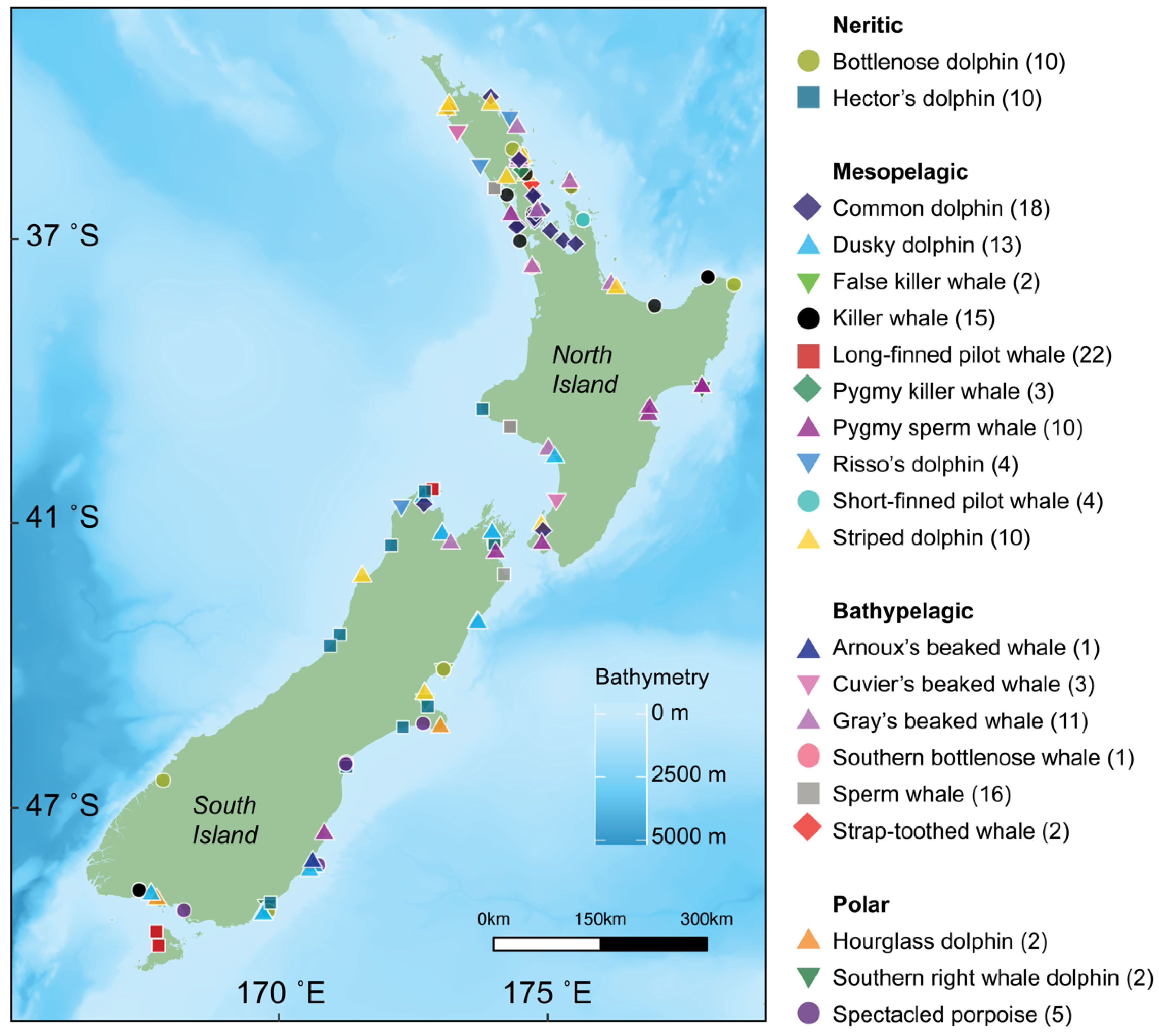
2.1. Sample Collection
2.2. Stable Isotope Analysis
2.3. Lipid Extraction
2.4. Analysis
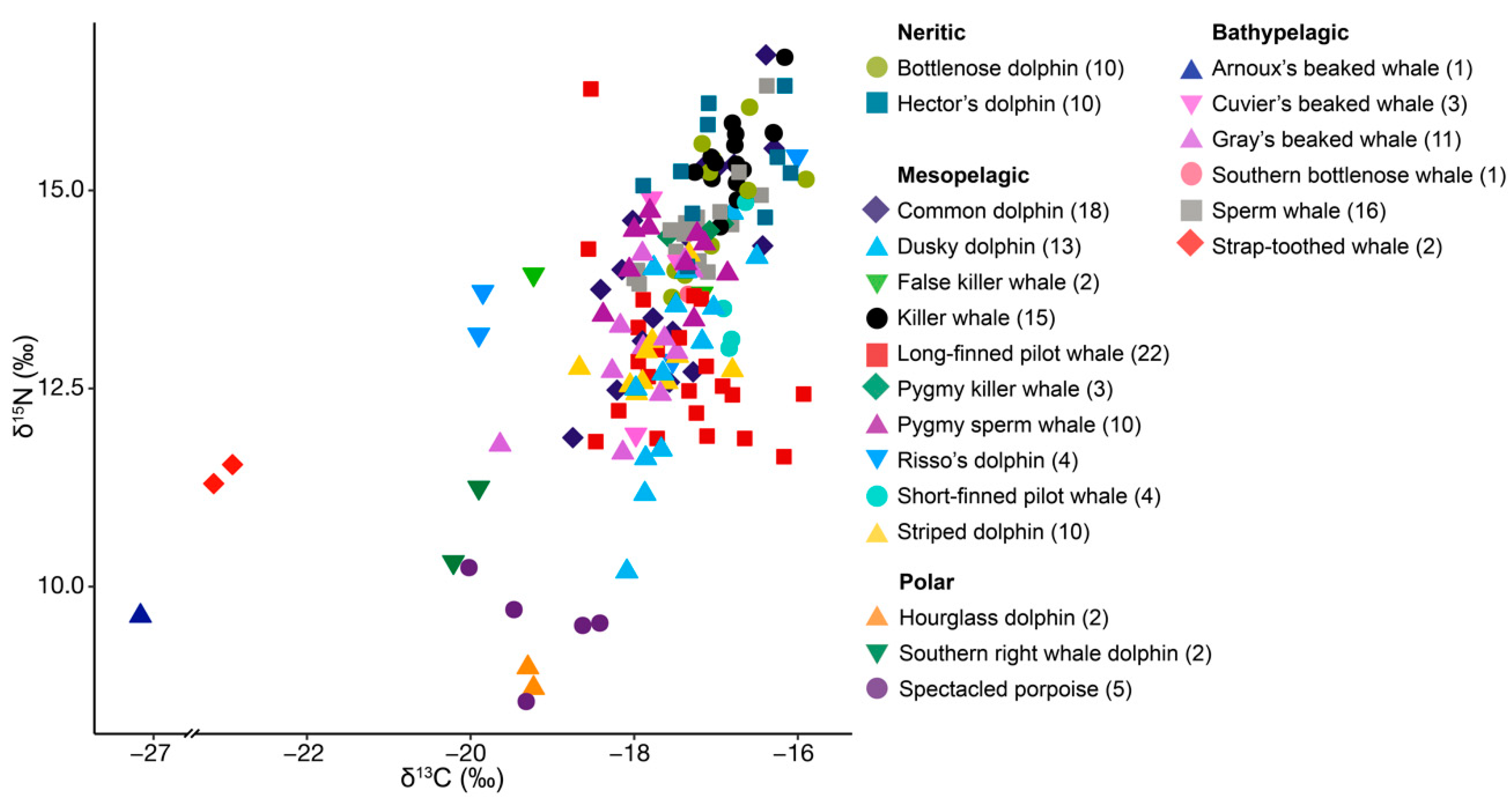
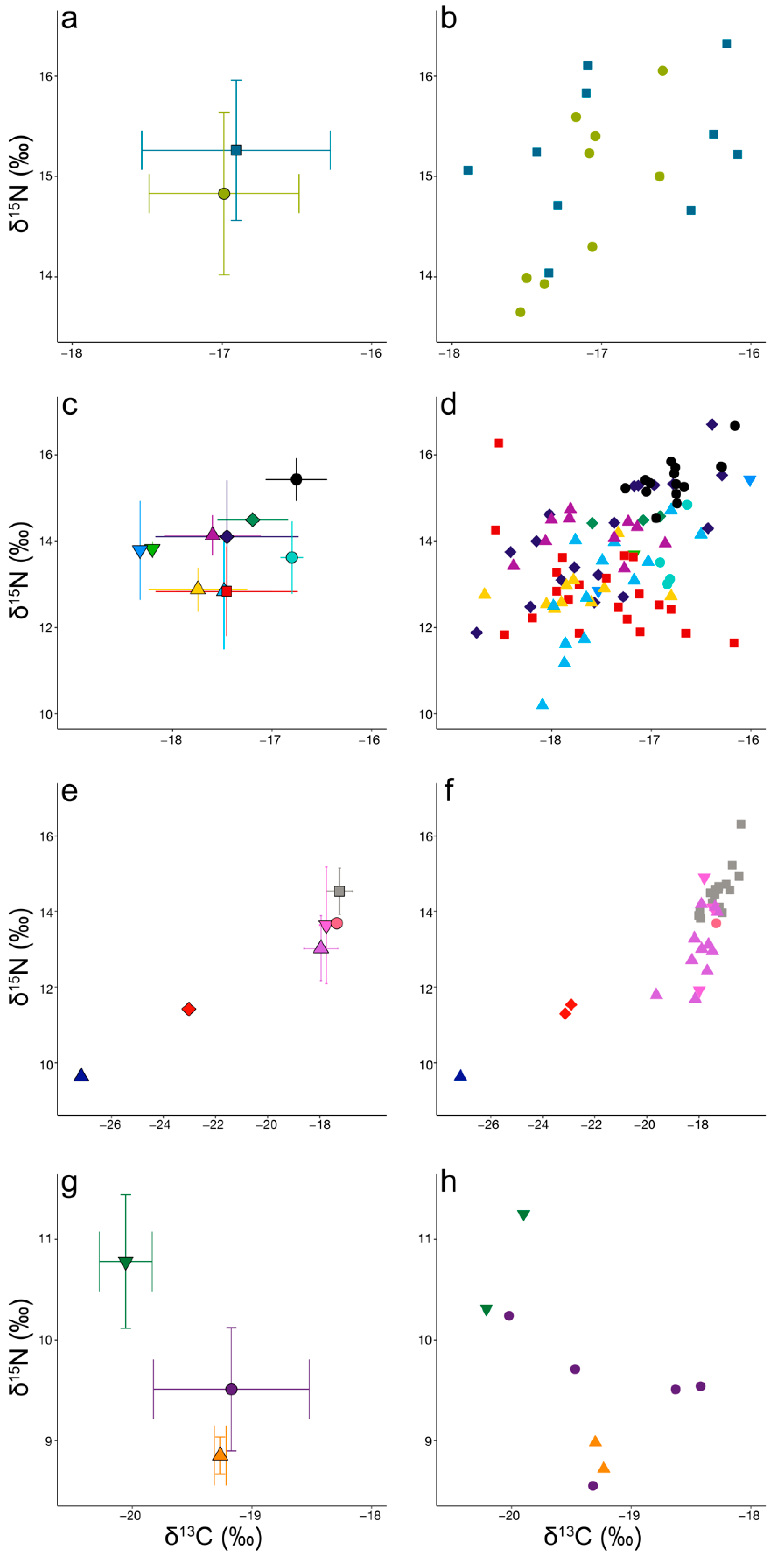
3. Results
3.1. Neritic Group
3.2. Mesopelagic Group
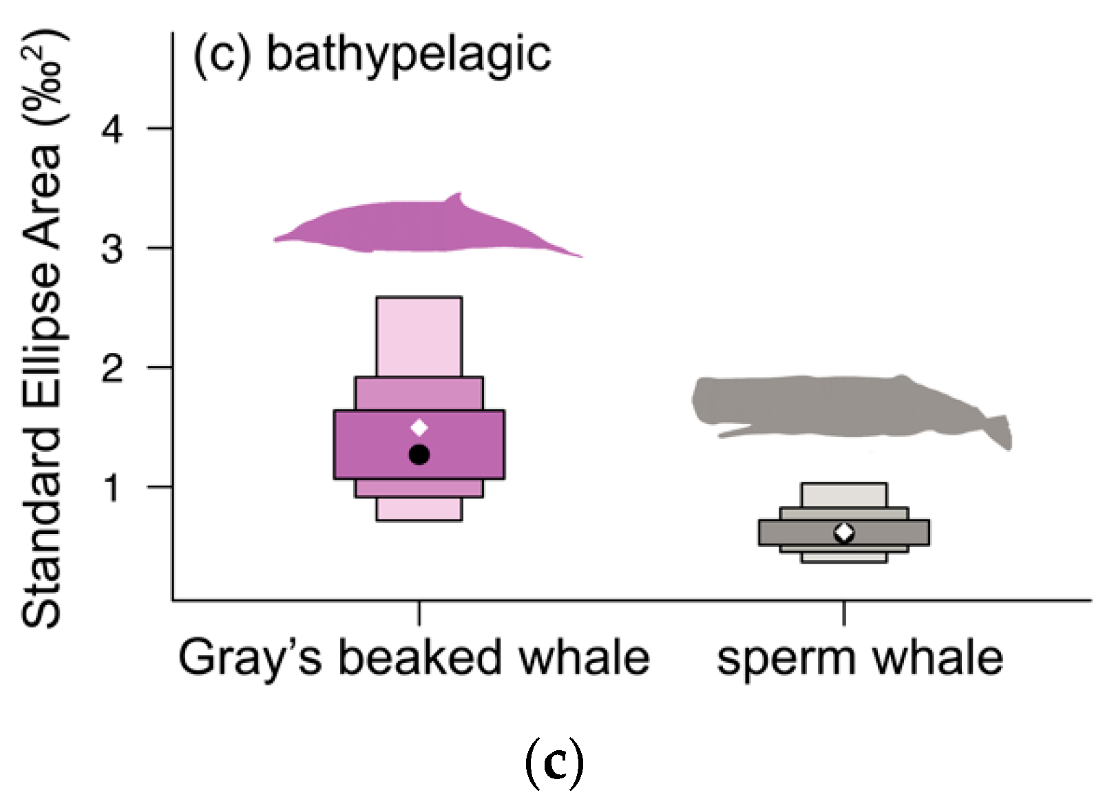
3.3. Bathypelagic Group
3.4. Polar Group
4. Discussion
4.1. Neritic Group
4.2. Mesopelagic Group
4.3. Bathypelagic Group
4.4. Polar Group
5. Conclusions
Author Contributions
Funding
Institutional Review Board Statement
Informed Consent Statement
Data Availability Statement
Acknowledgments
Conflicts of Interest
Appendix A. Extended Methods
Appendix A.1. Molecular Sexing
Appendix A.2. Mathematical Lipid Correction
Appendix A.3. Details on Layman Metrics
- (1)
- δ15N range: distance between the highest and lowest δ15N values (i.e., max δ15N—min δ15N). Measure of trophic length of the community.
- (2)
- δ13C range: distance between the highest and lowest δ13C values (i.e., max δ13C—min δ13C). Estimates the diversity of basal resources.
- (3)
- Total area (TA): total area of the convex hull comprising all data points. Measure of the total amount of niche space occupied and an indication of niche width.
- (4)
- Mean distance to centroid (CD): average Euclidean distance of each sample to the centroid. Measure of niche width and sample spacing.
- (5)
- Mean nearest neighbour distance (MNND): mean of the Euclidean distances to each sample’s nearest neighbour. Measure of the density and clustering of individuals.
- (6)
- Standard deviation of nearest neighbour distance (SDNND): measure of the evenness of spatial density and the packing of individuals. Low SDNND values indicate a more even distribution of trophic niches.

| δ15N | BD | HD | CD | DD | KW | LPW | PSW | SD | GW | SW |
|---|---|---|---|---|---|---|---|---|---|---|
| δ13C | ||||||||||
| BD | 0.106 | |||||||||
| HD | 0.373 | |||||||||
| CD | 0.007 | 0.001 | 0.001 | 0.473 | 0.003 | |||||
| DD | 0.451 | <0.001 | 0.494 | 0.005 | 0.463 | |||||
| KW | 0.001 | <0.001 | <0.001 | <0.001 | <0.001 | |||||
| LPW | 0.496 | 0.446 | 0.001 | 0.001 | 0.485 | |||||
| PSW | 0.286 | 0.294 | <0.001 | 0.288 | <0.001 | |||||
| SD | 0.134 | 0.104 | <0.001 | 0.132 | 0.256 | |||||
| GW | <0.001 | |||||||||
| SW | 0.001 |


References
- Hutchinson, G.E. A Treatise on Limnology; Wiley: New York, NY, USA, 1957; Volume 1, p. 243. [Google Scholar]
- Gause, G.F. The Struggle for Existence: A Classic of Mathematical Biology and Ecology; Williams & Wilkins Company: Baltimore, MD, USA, 1934. [Google Scholar]
- Arrizabalaga-Escudero, A.; Garin, I.; García-Mudarra, J.L.; Alberdi, A.; Aihartza, J.; Goiti, U. Trophic requirements beyond foraging habitats: The importance of prey source habitats in bat conservation. Biol. Conserv. 2015, 191, 512–519. [Google Scholar] [CrossRef] [Green Version]
- Tucker, A.D.; Fitzsimmons, N.N.; Gibbons, J.W. Resource partitioning by the estuarine turtle Malaclemys terrapin: Trophic, spatial, and temporal foraging constraints. Herpetologica 1995, 51, 167–181. [Google Scholar]
- Mèndez-Fernandez, P.; Bustamante, P.; Bode, A.; Chouvelon, T.; Ferreira, M.; Lopez, A.; Pierce, G.J.; Santos, M.B.; Spitz, J.; Vingada, J.V. Foraging ecology of five toothed whale species in the Northwest Iberian Peninsula, inferred using carbon and nitrogen isotope ratios. J. Exp. Mar. Biol. Ecol. 2012, 413, 150–158. [Google Scholar] [CrossRef] [Green Version]
- Teixeira, C.R.; Botta, S.; Daura-Jorge, F.G.; Pereira, L.B.; Newsome, S.D.; Simões-Lopes, P.C. Niche overlap and diet composition of three sympatric coastal dolphin species in the southwest Atlantic Ocean. Mar. Mammal Sci. 2020, 37, 111–126. [Google Scholar] [CrossRef]
- Giménez, J.; Cañadas, A.; Ramírez, F.; Afán, I.; García-Tiscar, S.; Fernández-Maldonado, C.; Castillo, J.J.; de Stephanis, R. Intra-and interspecific niche partitioning in striped and common dolphins inhabiting the southwestern Mediterranean Sea. Mar. Ecol. Prog. Ser. 2017, 567, 199–210. [Google Scholar] [CrossRef]
- Méndez-Fernandez, P.; Pierce, G.J.; Bustamante, P.; Chouvelon, T.; Ferreira, M.; González, A.F.; López, A.; Read, F.L.; Santos, M.B.; Spitz, J.; et al. Ecological niche segregation among five toothed whale species off the NW Iberian Peninsula using ecological tracers as multi-approach. Mar. Biol. 2013, 160, 2825–2840. [Google Scholar] [CrossRef] [Green Version]
- Newsome, S.D.; del Rio, C.M.; Bearhop, S.; Phillips, D.L. A niche for isotopic ecology. Front. Ecol. Environ. 2007, 5, 429–436. [Google Scholar] [CrossRef]
- Fry, B.; Sherr, E. 13C measurements as indicators of carbon flow in marine food webs. Contrib. Mar. Sci. 1984, 27, 15–47. [Google Scholar]
- Rounick, J.; Winterbourn, M. Stable carbon isotopes and carbon flow in ecosystems. Bioscience 1986, 36, 171–177. [Google Scholar] [CrossRef]
- Peterson, B.J.; Fry, B. Stable isotopes in ecosystem studies. Annu. Rev. Ecol. Syst. 1987, 18, 293–320. [Google Scholar] [CrossRef]
- Minagawa, M.; Wada, E. Stepwise enrichment of 15N along food chains: Further evidence and the relation between δ15N and animal age. Geochim. Cosmochim. Acta 1984, 48, 1135–1140. [Google Scholar] [CrossRef]
- Post, D.M. Using stable isotopes to estimate trophic position: Models, methods, and assumptions. Ecology 2002, 83, 703–718. [Google Scholar] [CrossRef]
- Browning, N.E.; McCulloch, S.D.; Bossart, G.D.; Worthy, G.A.J. Fine-scale population structure of estuarine bottlenose dolphins (Tursiops truncatus) assessed using stable isotope ratios and fatty acid signature analyses. Mar. Biol. 2014, 161, 1307–1317. [Google Scholar] [CrossRef]
- Giménez, J.; Ramírez, F.; Forero, M.G.; Almunia, J.; de Stephanis, R.; Navarro, J. Lipid effects on isotopic values in bottlenose dolphins (Tursiops truncatus) and their prey with implications for diet assessment. Mar. Biol. 2017, 164, 122. [Google Scholar] [CrossRef]
- Loizaga de Castro, R.; Saporiti, F.; Vales, D.G.; García, N.A.; Cardona, L.; Crespo, E.A. What are you eating? A stable isotope insight into the trophic ecology of short-beaked common dolphins in the Southwestern Atlantic Ocean. Mamm. Biol. 2016, 81, 571–578. [Google Scholar] [CrossRef]
- Giménez, J.; Marçalo, A.; Ramírez, F.; Verborgh, P.; Gauffier, P.; Esteban, R.; Nicolau, L.; González-Ortegón, E.; Baldó, F.; Vilas, C. Diet of bottlenose dolphins (Tursiops truncatus) from the Gulf of Cadiz: Insights from stomach content and stable isotope analyses. PLoS ONE 2017, 12, e0184673. [Google Scholar] [CrossRef] [Green Version]
- Stephenson, F.; Goetz, K.; Sharp, B.R.; Mouton, T.L.; Beets, F.L.; Roberts, J.; MacDiarmid, A.B.; Constantine, R.; Lundquist, C.J.; Sarmento Cabral, J. Modelling the spatial distribution of cetaceans in New Zealand waters. Divers. Distrib. 2020, 26, 495–516. [Google Scholar] [CrossRef]
- Baker, C.; Boren, L.; Childerhouse, S.; Constantine, R.; van Helden, A.; Lundquist, D.; Rolfe, J. Conservation Status of New Zealand Marine Mammals, 2019; New Zealand Threat Classification Series 29; Department of Conservation: Wellington, New Zealand, 2019.
- Bradford-Grieve, J.M.; Lewis, K.B.; Stanton, B.R. Advances in New Zealand oceanography, 1967–1991. N. Z. J. Mar. Freshw. Res. 1991, 25, 429–441. [Google Scholar] [CrossRef]
- Stevens, C.L.; O’Callaghan, J.M.; Chiswell, S.M.; Hadfield, M.G. Physical oceanography of New Zealand/Aotearoa shelf seas—A review. N. Z. J. Mar. Freshw. Res. 2019, 5, 6–45. [Google Scholar] [CrossRef] [Green Version]
- Schoener, T.W. Resource partitioning in ecological communities. Science 1974, 185, 27–39. [Google Scholar] [CrossRef]
- Pianka, E.R. Guild structure in desert lizards. Oikos 1980, 35, 194–201. [Google Scholar] [CrossRef]
- Arlettaz, R. Habitat selection as a major resource partitioning mechanism between the two sympatric sibling bat species Myotis myotis and Myotis blythii. J. Anim. Ecol. 1999, 68, 460–471. [Google Scholar] [CrossRef] [Green Version]
- Friedlaender, A.S.; Lawson, G.L.; Halpin, P.N. Evidence of resource partitioning between humpback and minke whales around the western Antarctic Peninsula. Mar. Mammal Sci. 2009, 25, 402–415. [Google Scholar] [CrossRef] [Green Version]
- Betty, E.L.; Bollard, B.; Murphy, S.; Ogle, M.; Hendriks, H.; Orams, M.B.; Stockin, K.A. Using emerging hot spot analysis of stranding records to inform conservation management of a data-poor cetacean species. Biodivers. Conserv. 2020, 29, 643–665. [Google Scholar] [CrossRef]
- Stockin, K.A.; Duignan, P.J.; Roe, W.D.; Meynier, L.; Alley, M.; Fettermann, T. Causes of mortality in stranded common dolphins (Delphinus sp.) from New Zealand waters between 1998 and 2008. Pac. Conserv. Biol. 2009, 15, 217–227. [Google Scholar] [CrossRef]
- Brabyn, M.W.; McLean, I.G. Oceanography and coastal topography of herd-stranding sites for whales in New Zealand. J. Mammal. 1992, 73, 469–476. [Google Scholar] [CrossRef]
- IJsseldijk, L.L.; Brownlow, A.C.; Mazzariol, S. Best Practice on Cetacean Post Mortem Investigation and Tissue Sampling. 2019. Available online: https://scholar.google.co.jp/scholar?q=Best+practice+on+cetacean+post+mortem+investigation+and+tissue+sampling&hl=ja&as_sdt=0&as_vis=1&oi=scholart (accessed on 1 August 2022).
- Geraci, J.R.; Lounsbury, V.J. Marine Mammals Ashore: A Field Guide for Strandings; National Aquarium in Baltimore: Baltimore, MD, USA, 2005. [Google Scholar]
- Jefferson, T.A.; Webber, M.A.; Pitman, R. Marine Mammals of the World: A Comprehensive Guide to Their Identification; Elsevier: Amsterdam, The Netherlands, 2011. [Google Scholar]
- Charting Around New Zaland (CANZ). New Zealand Region Bathymetry, 1:4,000,000, 2nd ed.; NIWA Chart Miscellaneous Series No. 85; National Institute of Water and Atmospheric Research (NIWA): Wellington, New Zealand, 2008. [Google Scholar]
- Wells, R.S.; Scott, M.D. Bottlenose dolphin, Tursiops truncatus, common bottlenose dolphin. In Encyclopedia of Marine Mammals; Würsig, B., Thewissen, J.G.M., Kovacs, K.M., Eds.; Academic Press: London, UK, 2018; pp. 118–125. [Google Scholar]
- Dawson, S.M. Cephalorhynchus dolphins: C. heavisidii, C. eutropia, C. hectori, and C. commersonii. In Encyclopedia of Marine Mammals; Würsig, B., Thewissen, J.G.M., Kovacs, K.M., Eds.; Academic Press: London, UK, 2018; pp. 166–172. [Google Scholar]
- Stockin, K.A.; Orams, M. The status of common dolphins (Delphinus delphis) within New Zealand waters. J. Cetacean Res. Manag. 2009, SC/61/SM20, 1–13. [Google Scholar]
- Van Waerebeek, K.; Würsig, B. Dusky dolphin: Lagenorhynchus obscurus. In Encyclopedia of Marine Mammals; Würsig, B., Thewissen, J.G.M., Kovacs, K.M., Eds.; Academic Press: London, UK, 2018; pp. 277–280. [Google Scholar]
- Baird, R.W. False killer whale: Pseudorca crassidens. In Encyclopedia of Marine Mammals; Würsig, B., Thewissen, J., Kovacs, K.M., Eds.; Academic Press: London, UK, 2018; pp. 347–349. [Google Scholar]
- Ford, J.K.B. Killer whale: Orcinus orca. In Encyclopedia of Marine Mammals; Würsig, B., Thewissen, J.G.M., Kovacs, K.M., Eds.; Academic Press: London, UK, 2018; pp. 531–537. [Google Scholar]
- Olson, P.A. Pilot whales: Globicephala melas and G. macrorhynchus. In Encyclopedia of Marine Mammals; Würsig, B., Thewissen, J.G.M., Kovacs, K.M., Eds.; Academic Press: London, UK, 2018; pp. 701–705. [Google Scholar]
- Baird, R.W. Pygmy killer whale: Feresa attenuata. In Encyclopedia of Marine Mammals; Würsig, B., Thewissen, J.G.M., Kovacs, K.M., Eds.; Academic Press: London, UK, 2018; pp. 788–790. [Google Scholar]
- McAlpine, D.F. Pygmy and dwarf sperm whales: Kogia breviceps and K. sima. In Encyclopedia of Marine Mammals; Elsevier: Amsterdam, The Netherlands, 2018; pp. 786–788. [Google Scholar]
- Baird, R.W. Risso’s dolphin: Grampus griseus. In Encyclopedia of Marine Mammals; Würsig, B., Thewissen, J.G.M., Kovacs, K.M., Eds.; Academic Press: London, UK, 2018; pp. 824–827. [Google Scholar]
- Archer, F.I. Striped dolphin: Stenella coeruleoalba. In Encyclopedia of Marine Mammals; Würsig, B., Thewissen, J.G.M., Kovacs, K.M., Eds.; Academic Press: London, UK, 2018; pp. 954–956. [Google Scholar]
- Thewissen, J. Berardius beaked whales: Berardius bairdii and B. arnuxii. In Encyclopedia of Marine Mammals; Elsevier: Amsterdam, The Netherlands, 2018; pp. 97–99. [Google Scholar]
- Baird, R.W. Cuvier’s beaked whale: Ziphius cavirostris. In Encyclopedia of Marine Mammals; Würsig, B., Thewissen, J.G.M., Kovacs, K.M., Eds.; Academic Press: London, UK, 2018; pp. 234–237. [Google Scholar]
- Patel, S.; Thompson, K.F.; Santure, A.W.; Constantine, R.; Millar, C.D. Genetic Kinship analyses reveal that Gray’s beaked whales strand in unrelated groups. J. Hered. 2017, 108, 456–461. [Google Scholar] [CrossRef]
- Thompson, K.F.; Ruggiero, K.; Millar, C.D.; Constantine, R.; van Helden, A.L. Large-scale multivariate analysis reveals sexual dimorphism and geographic differences in the Gray’s beaked whale. J. Zool. 2014, 294, 13–21. [Google Scholar] [CrossRef]
- Moors-Murphy, H.B. Bottlenose Whales: Hyperoodon ampullatus and H. planifrons. In Encyclopedia of Marine Mammals; Elsevier: Amsterdam, The Netherlands, 2018; pp. 130–132. [Google Scholar]
- Whitehead, H. Sperm whale: Physeter macrocephalus. In Encyclopedia of Marine Mammals; Würsig, B., Thewissen, J.G.M., Kovacs, K.M., Eds.; Academic Press: London, UK, 2018; pp. 919–925. [Google Scholar]
- Pitman, R. Mesoplodon beaked whales: Mesoplodon spp. In Encyclopedia of Marine Mammals; Würsig, B., Thewissen, J.G.M., Kovacs, K.M., Eds.; Academic Press: London, UK, 2018; pp. 788–790. [Google Scholar]
- Cipriano, F. Hourglass dolphin: Lagenorhynchus cruciger. In Encyclopedia of Marine Mammals; Würsig, B., Thewissen, J.G.M., Kovacs, K.M., Eds.; Academic Press: London, UK, 2018; pp. 480–483. [Google Scholar]
- Lipsky, J.D.; Brownell Jr, R.L. Right Whale Dolphins: Lissodelphis borealis and L. peronii. In Encyclopedia of Marine Mammals; Elsevier: Amsterdam, The Netherlands, 2018; pp. 813–817. [Google Scholar]
- Goodall, R.N.P.; Brownell, R.L., Jr. Spectacled porpoise: Phocoena dioptrica. In Encyclopedia of Marine Mammals; Würsig, B., Thewissen, J.G.M., Kovacs, K.M., Eds.; Academic Press: London, UK, 2018; pp. 912–916. [Google Scholar]
- Peters, K.J.; Bury, S.J.; Betty, E.L.; Parra, G.J.; Tezanos-Pinto, G.; Stockin, K.A. Foraging ecology of the common dolphin Delphinus delphis revealed by stable isotope analysis. Mar. Ecol. Prog. Ser. 2020, 652, 173–186. [Google Scholar] [CrossRef]
- Ryan, C.; McHugh, B.; Trueman, C.N.; Harrod, C.; Berrow, S.D.; O’Connor, I. Accounting for the effects of lipids in stable isotope (δ13C and δ15N values) analysis of skin and blubber of balaenopterid whales. Rapid Commun. Mass Spectrom. 2012, 26, 2745–2754. [Google Scholar] [CrossRef] [PubMed]
- Lesage, V.; Morin, Y.; Rioux, È.; Pomerleau, C.; Ferguson, S.H.; Pelletier, É. Stable isotopes and trace elements as indicators of diet and habitat use in cetaceans: Predicting errors related to preservation, lipid extraction, and lipid normalization. Mar. Ecol. Prog. Ser. 2010, 419, 249–265. [Google Scholar] [CrossRef]
- DeNiro, M.J.; Epstein, S. Influence of diet on the distribution of carbon isotopes in animals. Geochim. Cosmochim. Acta 1978, 42, 495–506. [Google Scholar] [CrossRef]
- Skinner, M.M.; Martin, A.A.; Moore, B.C. Is lipid correction necessary in the stable isotope analysis of fish tissues? Rapid Commun. Mass Spectrom. 2016, 30, 881–889. [Google Scholar] [CrossRef] [PubMed]
- Post, D.; Layman, C.; Arrington, D.A.; Takimoto, G.; Quattrochi, J.; Montaña, C. Getting to the fat of the matter: Models, methods and assumptions for dealing with lipids in stable isotope analyses. Oecologia 2007, 152, 179–189. [Google Scholar] [CrossRef]
- Yurkowski, D.J.; Hussey, N.E.; Semeniuk, C.; Ferguson, S.H.; Fisk, A.T. Effects of lipid extraction and the utility of lipid normalization models on δ13C and δ15N values in Arctic marine mammal tissues. Polar Biol. 2015, 38, 131–143. [Google Scholar] [CrossRef]
- Groß, J.; Fry, B.; Burford, M.A.; Bengtson Nash, S. Assessing the effects of lipid extraction and lipid correction on stable isotope values (δ13C and δ15N) of blubber and skin from southern hemisphere humpback whales. Rapid Commun. Mass Spectrom. 2021, 35, e9140. [Google Scholar] [CrossRef]
- Ricca, M.; Miles, A.; Anthony, R.; Deng, X.; Hung, S. Effect of lipid extraction on analyses of stable carbon and stable nitrogen isotopes in coastal organisms of the Aleutian archipelago. Can. J. Zool. 2007, 85, 40–48. [Google Scholar] [CrossRef]
- Mintenbeck, K.; Brey, T.; Jacob, U.; Knust, R.; Struck, U. How to account for the lipid effect on carbon stable-isotope ratio (δ13C): Sample treatment effects and model bias. J. Fish. Biol. 2008, 72, 815–830. [Google Scholar] [CrossRef] [Green Version]
- Quay, P.; Sonnerup, R.; Westby, T.; Stutsman, J.; McNichol, A. Changes in the 13C/12C of dissolved inorganic carbon in the ocean as a tracer of anthropogenic CO2 uptake. Glob. Biogeochem. Cycles 2003, 17, 4-1–4-20. [Google Scholar] [CrossRef]
- Keeling, C.D.; Mook, W.G.; Tans, P.P. Recent trends in the 13C/12C ratio of atmospheric carbon dioxide. Nature 1979, 277, 121. [Google Scholar] [CrossRef]
- Manly, B.F.J. Randomization, Bootstrap and Monte Carlo Methods in Biology, 2nd ed.; Chapman and Hall: London, UK, 1997. [Google Scholar]
- Jackson, M.C.; Donohue, I.; Jackson, A.L.; Britton, J.R.; Harper, D.M.; Grey, J. Population-level metrics of trophic structure based on stable isotopes and their application to invasion ecology. PLoS ONE 2012, 7, e31757. [Google Scholar] [CrossRef]
- Jackson, A.L.; Inger, R.; Parnell, A.C.; Bearhop, S. Comparing isotopic niche widths among and within communities: SIBER—Stable Isotope Bayesian Ellipses in R. J. Anim. Ecol. 2011, 80, 595–602. [Google Scholar] [CrossRef] [PubMed]
- R Core Team. R: A Language and Environment for Statistical Computing; R Foundation for Statistical Computing: Vienna, Austria, 2022; Available online: https://www.R-project.org/:2022 (accessed on 1 August 2022).
- Miller, E.; Lalas, C.; Dawson, S.; Ratz, H.; Slooten, E. Hector’s dolphin diet: The species, sizes and relative importance of prey eaten by Cephalorhynchus hectori, investigated using stomach content analysis. Mar.Mammal Sci. 2013, 29, 606–628. [Google Scholar] [CrossRef]
- Rayment, W.; Webster, T. Observations of Hector’s dolphins (Cephalorhynchus hectori) associating with inshore fishing trawlers at Banks Peninsula, New Zealand. N. Z. J. Mar. Freshw. Res. 2009, 43, 911–916. [Google Scholar] [CrossRef] [Green Version]
- Baker, C.; Chilvers, B.; Constantine, R.; DuFresne, S.; Mattlin, R.; Van Helden, A.; Hitchmough, R. Conservation status of New Zealand marine mammals (suborders Cetacea and Pinnipedia), 2009. N. Z. J. Mar. Freshw. Res. 2010, 44, 101–115. [Google Scholar] [CrossRef] [Green Version]
- Zaeschmar, J.R.; Tezanos-Pinto, G.; Dwyer, S.L.; Peters, C.H.; Berghan, J.; Donnelly, D.; Meissner, A.M.; Visser, I.N.; Weir, J.S.; Judkins, A.G. Occurrence, site fidelity, and associations of oceanic common bottlenose dolphins (Tursiops truncatus) off northeastern New Zealand. Mar. Mammal Sci. 2020, 36, 1180–1195. [Google Scholar] [CrossRef]
- Lusseau, S.M.; Wing, S.R. Importance of local production versus pelagic subsidies in the diet of an isolated population of bottlenose dolphins Tursiops sp. Mar. Ecol. Prog. Ser. 2006, 321, 283–293. [Google Scholar] [CrossRef] [Green Version]
- Moreno, R.; Jover, L.; Munilla, I.; Velando, A.; Sanpera, C. A three-isotope approach to disentangling the diet of a generalist consumer: The yellow-legged gull in northwest Spain. Mar. Biol. 2010, 157, 545–553. [Google Scholar] [CrossRef]
- Ramírez, F.; Abdennadher, A.; Sanpera, C.; Jover, L.; Wassenaar, L.I.; Hobson, K.A. Assessing waterbird habitat use in coastal evaporative systems using stable isotopes (δ13C, δ15N and δD) as environmental tracers. Estuar. Coast. Shelf Sci. 2011, 92, 217–222. [Google Scholar] [CrossRef]
- Parra, G.J.; Wojtkowiak, Z.; Peters, K.J.; Cagnazzi, D. Isotopic niche overlap between sympatric Australian snubfin and humpback dolphins. Ecol. Evol. 2022, 12, e8937. [Google Scholar] [CrossRef] [PubMed]
- Meynier, L.; Stockin, K.; Bando, M.; Duignan, P. Stomach contents of common dolphin (Delphinus sp.) from New Zealand waters. N. Z. J. Mar. Freshw. Res. 2008, 42, 257–268. [Google Scholar] [CrossRef]
- Pusineri, C.; Magnin, V.; Meynier, L.; Spitz, J.; Hassani, S.; Ridoux, V. Food and feeding ecology of the common dolphin (Delphinus delphis) in the oceanic northeast atlantic and comparison with its diet in neritic areas. Mar. Mammal Sci. 2007, 23, 30–47. [Google Scholar] [CrossRef]
- Silva, M. Diet of common dolphins, Delphinus delphis, off the Portuguese continental coast. J. Mar. Biol. Assoc. UK 1999, 79, 531–540. [Google Scholar] [CrossRef]
- Stockin, K.A.; Pierce, G.J.; Binedell, V.; Wiseman, N.; Orams, M.B. Factors affecting the occurrence and demographics of common dolphins (Delphinus sp.) in the Hauraki Gulf, New Zealand. Aquat. Mamm. 2008, 34, 200–211. [Google Scholar] [CrossRef] [Green Version]
- Hinton, B.; Stockin, K.A.; Bury, S.J.; Peters, K.J.; Betty, E.l. Trophic niche analysis of long-finned pilot whales (Globicephala melas edwardii) in New Zealand waters. Biology, 2022; accepted. [Google Scholar]
- Beasley, I.; Cherel, Y.; Robinson, S.; Betty, E.; Hagihara, R.; Gales, R. Stomach contents of long-finned pilot whales, Globicephala melas mass-stranded in Tasmania. PLoS ONE 2019, 14, e0206747. [Google Scholar] [CrossRef]
- Beatson, E.; O’Shea, S.; Ogle, M. First report on the stomach contents of long-finned pilot whales, Globicephala melas, stranded in New Zealand. N. Z. J. Zool. 2007, 34, 51–56. [Google Scholar] [CrossRef]
- Hinton, B.; Stockin, K.A.; Betty, E.L. Intraspecific dietary variation of long-finned pilot whales (Globicephala melas edwardii) stranded on the Aotearoa, New Zealand coast. Mar. Biol. 2022; accepted. [Google Scholar]
- Luna, A.; Sánchez, P.; Chicote, C.; Gazo, M. Cephalopods in the diet of Risso’s dolphin (Grampus griseus) from the Mediterranean Sea: A review. Mar. Mammal Sci. 2021, 38, 725–741. [Google Scholar] [CrossRef]
- Stockin, K.A.; Amiot, C.; Meynier, L.M.; Purvin, C.; Machovsky-Capuska, G.E. A duplex lens: Understanding common dolphin and Australasian gannet feeding associations from an ethological and nutritional perspective. ICES J. Mar. 2022. [Google Scholar] [CrossRef]
- Meissner, A.M.; MacLeod, C.D.; Richard, P.; Ridoux, V.; Pierce, G. Feeding ecology of striped dolphins, Stenella coeruleoalba, in the north-western Mediterranean Sea based on stable isotope analyses. J. Mar. Biol. Assoc. UK 2012, 92, 1677–1687. [Google Scholar] [CrossRef] [Green Version]
- Spitz, J.; Richard, E.; Meynier, L.; Pusineri, C.; Ridoux, V. Dietary plasticity of the oceanic striped dolphin, Stenella coeruleoalba, in the neritic waters of the Bay of Biscay. J. Sea Res. 2006, 55, 309–320. [Google Scholar] [CrossRef]
- Ringelstein, J.; Pusineri, C.; Hassani, S.; Meynier, L.; Nicolas, R.; Ridoux, V. Food and feeding ecology of the striped dolphin, Stenella coeruleoalba, in the oceanic waters of the north-east Atlantic. J. Mar. Biol. Assoc. UK 2006, 86, 909–918. [Google Scholar] [CrossRef]
- Würtz, M.; Marrale, D. Food of striped dolphin, Stenella coeruleoalba, in the Ligurian Sea. J. Mar. Biol. Assoc. UK 1993, 73, 571–578. [Google Scholar] [CrossRef]
- McFadden, C.J. Behavioral Flexibility of Feeding Dusky Dolphins (Lagenorhynchus obscurus) in Admiralty Bay, New Zealand; Texas A&M University: College Station, TX, USA, 2004. [Google Scholar]
- Vaughn, R.L.; Shelton, D.E.; Timm, L.L.; Watson, L.A.; Würsig, B. Dusky dolphin (Lagenorhynchus obscurus) feeding tactics and multi-species associations. N. Z. J. Mar. Freshw. Res. 2007, 41, 391–400. [Google Scholar] [CrossRef] [Green Version]
- Markowitz, T.M. Social Organization of the New Zealand Dusky Dolphin; Texas A&M University: College Station, TX, USA, 2004. [Google Scholar]
- Beatson, E. The diet of pygmy sperm whales, Kogia breviceps, stranded in New Zealand: Implications for conservation. Rev. Fish. Biol. Fish. 2007, 17, 295–303. [Google Scholar] [CrossRef]
- West, K.; Walker, W.; Baird, R.; White, W.; Levine, G.; Brown, E.; Schofield, D. Diet of pygmy sperm whales (Kogia breviceps) in the Hawaiian Archipelago. Mar. Mammal Sci. 2009, 25, 931–943. [Google Scholar] [CrossRef] [Green Version]
- Spitz, J.; Cherel, Y.; Bertin, S.; Kiszka, J.; Dewez, A.; Ridoux, V. Prey preferences among the community of deep-diving odontocetes from the Bay of Biscay, Northeast Atlantic. Deep. Sea Res. Part I Oceanogr. Res. Pap. 2011, 58, 273–282. [Google Scholar] [CrossRef]
- Staudinger, M.D.; McAlarney, R.J.; McLellan, W.A.; Ann Pabst, D. Foraging ecology and niche overlap in pygmy (Kogia breviceps) and dwarf (Kogia sima) sperm whales from waters of the US mid-Atlantic coast. Mar. Mammal Sci. 2014, 30, 626–655. [Google Scholar] [CrossRef]
- Meynier, L.; Pusineri, C.; Spitz, J.; Santos, M.B.; Pierce, G.J.; Ridoux, V. Intraspecific dietary variation in the short-beaked common dolphin Delphinus delphis in the Bay of Biscay: Importance of fat fish. Mar. Ecol. Prog. Ser. 2008, 354, 277–287. [Google Scholar] [CrossRef] [Green Version]
- Plön, S. The Status and Natural History of Pygmy (Kogia breviceps) and Dwarf (K. sima) Sperm Whales off Southern Africa; Rhodes University: Grahamstown, South Africa, 2004. [Google Scholar]
- Ford, J.K.; Ellis, G.M.; Barrett-Lennard, L.G.; Morton, A.B.; Palm, R.S.; Balcomb III, K.C. Dietary specialization in two sympatric populations of killer whales (Orcinus orca) in coastal British Columbia and adjacent waters. Can. J. Zool. 1998, 76, 1456–1471. [Google Scholar] [CrossRef] [Green Version]
- Ford, J.K.; Ellis, G.M. Selective foraging by fish-eating killer whales Orcinus orca in British Columbia. Mar. Ecol. Prog. Ser. 2006, 316, 185–199. [Google Scholar] [CrossRef] [Green Version]
- Andvik, C.; Jourdain, E.; Lyche, J.L.; Karoliussen, R.; Borga, K. High Levels of Legacy and Emerging Contaminants in Killer Whales (Orcinus orca) from Norway, 2015 to 2017. Environ. Toxicol. Chem. 2021, 40, 1848–1858. [Google Scholar] [CrossRef] [PubMed]
- Saulitis, E.; Matkin, C.; Barrett-Lennard, L.; Heise, K.; Ellis, G. Foraging strategies of sympatric killer whale (Orcinus orca) populations in Prince William Sound, Alaska. Mar. Mammal Sci. 2000, 16, 94–109. [Google Scholar] [CrossRef]
- Visser, I. Benthic foraging on stingrays by killer whales (Orcinus orca) in New Zealand waters. Mar. Mammal Sci. 1999, 15, 220–227. [Google Scholar] [CrossRef]
- Visser, I.N. First observations of feeding on thresher (Alopias vulpinus) and hammerhead (Sphyrna zygaena) sharks by killer whales (Orcinus orca) specialising on elasmobranch prey. Aquat. Mamm. 2005, 31, 83–88. [Google Scholar] [CrossRef]
- Visser, I.N.; Berghan, J.; van Meurs, R.; Fertl, D. Killer whale (Orcinus orca) predation on a shortfin mako shark (Isurus oxyrinchus) in New Zealand waters. Aquat. Mamm. 2000, 26, 229–231. [Google Scholar]
- Visser, I.N. A summary of interactions between orca (Orcinus orca) and other cetaceans in New Zealand waters. Ingrid N Viss. 1999, 24, 101–112. [Google Scholar]
- Jourdain, E.; Andvik, C.; Karoliussen, R.; Ruus, A.; Vongraven, D.; Borgå, K. Isotopic niche differs between seal and fish-eating killer whales (Orcinus orca) in northern Norway. Ecol. Evol. 2020, 10, 4115–4127. [Google Scholar] [CrossRef] [Green Version]
- Borisova, E.A.; Filatova, O.A.; Fedutin, I.D.; Tiunov, A.V.; Shpak, O.V.; Hoyt, E. Ecotype and geographical variation in carbon and nitrogen stable isotope values in western North Pacific killer whales (Orcinus orca). Mar. Mammal Sci. 2020, 36, 925–938. [Google Scholar] [CrossRef]
- Herman, D.; Burrows, D.; Wade, P.; Durban, J.; Matkin, C.; LeDuc, R.; Barrett-Lennard, L.; Krahn, M.M. Feeding ecology of eastern North Pacific killer whales Orcinus orca from fatty acid, stable isotope, and organochlorine analyses of blubber biopsies. Mar. Ecol. Prog. Ser. 2005, 302, 275–291. [Google Scholar] [CrossRef] [Green Version]
- Zaeschmar, J.R.; Dwyer, S.L.; Stockin, K.A. Rare observations of false killer whales (Pseudorca crassidens) cooperatively feeding with common bottlenose dolphins (Tursiops truncatus) in the Hauraki Gulf, New Zealand. Mar. Mammal Sci. 2013, 29, 555–562. [Google Scholar] [CrossRef]
- Zaeschmar, J.R.; Visser, I.N.; Fertl, D.; Dwyer, S.L.; Meissner, A.M.; Halliday, J.; Berghan, J.; Donnelly, D.; Stockin, K.A. Occurrence of false killer whales (Pseudorca crassidens) and their association with common bottlenose dolphins (Tursiops truncatus) off northeastern New Zealand. Mar. Mammal Sci. 2014, 30, 594–608. [Google Scholar] [CrossRef]
- Giménez, J.; Cañadas, A.; Ramírez, F.; Afán, I.; García-Tiscar, S.; Fernández-Maldonado, C.; Castillo, J.J.; de Stephanis, R. Living apart together: Niche partitioning among Alboran Sea cetaceans. Ecol. Indic. 2018, 95, 32–40. [Google Scholar] [CrossRef]
- MacKenzie, K.M.; Lydersen, C.; Haug, T.; Routti, H.; Aars, J.; Andvik, C.M.; Borgå, K.; Fisk, A.T.; Meier, S.; Biuw, M.; et al. Niches of marine mammals in the European Arctic. Ecol. Indic. 2022, 136, 108661. [Google Scholar] [CrossRef]
- MacLeod, C.D.; Santos, M.; Pierce, G.J. Review of data on diets of beaked whales: Evidence of niche separation and geographic segregation. J. Mar. Biol. Assoc. UK 2003, 83, 651–665. [Google Scholar] [CrossRef]
- Beatson, E. Stomach contents of beaked whales (Ziphiidae) stranded on the New Zealand coast. In Proceedings of the New Zealand Marine Sciences Society Conference, Auckland, New Zealand, 24—26 November 2009. [Google Scholar]
- Gómez-Villota, F. Sperm Whale Diet in New Zealand; Auckland University of Technology: Auckland, New Zealand, 2007. [Google Scholar]
- Palmer, E.; Alexander, A.; Liggins, L.; Guerra, M.; Bury, S.J.; Hendriks, H.; Stockin, K.A.; Peters, K.J. A piece of the puzzle: Analyses of recent strandings and historical records reveal new genetic and ecological insights on New Zealand sperm whales Mar. Ecol. Prog. Ser. 2022, 690, 201–217. [Google Scholar] [CrossRef]
- Clarke, M.; Roper, C. Cephalopods represented by beaks in the stomach of a sperm whale stranded at Paekakariki, North Island, New Zealand. Afr. J. Mar. Sci. 1998, 20, 1814–2338. [Google Scholar] [CrossRef] [Green Version]
- Guerra, M.; Wing, L.; Dawson, S.; Rayment, W. Stable isotope analyses reveal seasonal and inter-individual variation in the foraging ecology of sperm whales. Mar. Ecol. Prog. Ser. 2020, 638, 207–219. [Google Scholar] [CrossRef]
- Guerra, M.; Hickmott, L.; van der Hoop, J.; Rayment, W.; Leunissen, E.; Slooten, E.; Moore, M. Diverse foraging strategies by a marine top predator: Sperm whales exploit pelagic and demersal habitats in the Kaikōura submarine canyon. Deep. Sea Res. Part I Oceanogr. Res. Pap. 2017, 128, 98–108. [Google Scholar] [CrossRef] [Green Version]
- Riccialdelli, L.; Viola, M.N.P.; Panarello, H.O.; Goodall, R.N.P. Evaluating the isotopic niche of beaked whales from the southwestern South Atlantic and Southern Oceans. Mar. Ecol. Prog. Ser. 2017, 581, 183–198. [Google Scholar] [CrossRef] [Green Version]
- Sekiguchi, K.; Klages, N.; Findlay, K. Feeding habits and possible movements of southern bottlenose whales (Hyperoodon planifrons). Proc. NIPR Symp. Polar Biol. 1993, 6, 84–97. [Google Scholar]
- Fernández, R.; Pierce, G.J.; MacLeod, C.D.; Brownlow, A.; Reid, R.J.; Rogan, E.; Addink, M.; Deaville, R.; Jepson, P.D.; Santos, M.B. Strandings of northern bottlenose whales, Hyperoodon ampullatus, in the north-east Atlantic: Seasonality and diet. J. Mar. Biol. Assoc. UK 2014, 94, 1109–1116. [Google Scholar] [CrossRef]
- Santos, M.; Pierce, G.J.; Smeenk, C.; Addink, M.; Kinze, C.; Tougaard, S.; Herman, J. Stomach contents of northern bottlenose whales Hyperoodon ampullatus stranded in the North Sea. J. Mar. Biol. Assoc. UK 2001, 81, 143–150. [Google Scholar] [CrossRef]
- Hooker, S.K.; Iverson, S.J.; Ostrom, P.; Smith, S.C. Diet of northern bottlenose whales inferred from fatty-acid and stable-isotope analyses of biopsy samples. Can. J. Zool. 2001, 79, 1442–1454. [Google Scholar] [CrossRef]
- Sekiguchi, K.; Klages, N.; Best, P. The diet of strap-toothed whales (Mesoplodon layardii). J. Zool. 1996, 239, 453–463. [Google Scholar] [CrossRef]
- Goodall, R.; Baker, A.; Best, P.; Meyer, M.; Miyazaki, N. On the biology of the hourglass dolphin, Lagenorhynchus cruciger (Quoy and Gaimard, 1824). Rep. Int. Whal. Comm. 1997, 47, 985–999. [Google Scholar]
- Cherel, Y.; Hobson, K.A. Geographical variation in carbon stable isotope signatures of marine predators: A tool to investigate their foraging areas in the Southern Ocean. Mar. Ecol. Prog. Ser. 2007, 329, 281–287. [Google Scholar] [CrossRef] [Green Version]
- Riccialdelli, L.; Newsome, S.D.; Fogel, M.L.; Goodall, R.N.P. Isotopic assessment of prey and habitat preferences of a cetacean community in the southwestern South Atlantic Ocean. Mar. Ecol. Prog. Ser. 2010, 418, 235–248. [Google Scholar] [CrossRef] [Green Version]
- Browning, N.E.; Dold, C.J.I.F.; Worthy, G.A. Isotope turnover rates and diet-tissue discrimination in skin of ex situ bottlenose dolphins (Tursiops truncatus). J. Exp. Biol. 2014, 217, 214–221. [Google Scholar] [CrossRef] [Green Version]
- Giménez, J.; Ramírez, F.; Almunia, J.G.; Forero, M.; de Stephanis, R. From the pool to the sea: Applicable isotope turnover rates and diet to skin discrimination factors for bottlenose dolphins (Tursiops truncatus). J. Exp. Mar. Biol. Ecol. 2016, 475, 54–61. [Google Scholar] [CrossRef]
- Busquets-Vass, G.; Newsome, S.D.; Calambokidis, J.; Serra-Valente, G.; Jacobsen, J.K.; Aguíñiga-García, S.; Gendron, D. Estimating blue whale skin isotopic incorporation rates and baleen growth rates: Implications for assessing diet and movement patterns in mysticetes. PLoS ONE 2017, 12, e0177880. [Google Scholar] [CrossRef] [PubMed] [Green Version]
- Connolly, R.M.; Guest, M.A.; Melville, A.J.; Oakes, J.M. Sulfur stable isotopes separate producers in marine food-web analysis. Oecologia 2004, 138, 161–167. [Google Scholar] [CrossRef]
- Clementz, M.T.; Koch, P.L. Differentiating aquatic mammal habitat and foraging ecology with stable isotopes in tooth enamel. Oecologia 2001, 129, 461–472. [Google Scholar] [CrossRef] [PubMed]
- Shipley, O.N.; Matich, P. Studying animal niches using bulk stable isotope ratios: An updated synthesis. Oecologia 2020, 193, 27–51. [Google Scholar] [CrossRef] [PubMed]
- Rosel, P.E. PCR-based sex determination in Odontocete cetaceans. Conserv. Genet. 2003, 4, 647–649. [Google Scholar] [CrossRef]
- Richard, K.R.; McCarrey, S.W.; Wright, J.M. DNA sequence from the SRY gene of the sperm whale (Physeter macrocephalus) for use in molecular sexing. Can. J. Zool. 1994, 72, 873–877. [Google Scholar] [CrossRef]
- Bérubé, M.; Palsbøll, P. Identification of sex in cetaceans by multiplexing with three ZFX and ZFY specific primers. Mol. Ecol. 1996, 5, 283–287. [Google Scholar] [CrossRef]
- Layman, C.A.; Arrington, D.A.; Montaña, C.G.; Post, D.M. Can stable isotope ratios provide for community-wide measures of trophic structure? Ecology 2007, 88, 42–48. [Google Scholar] [CrossRef]


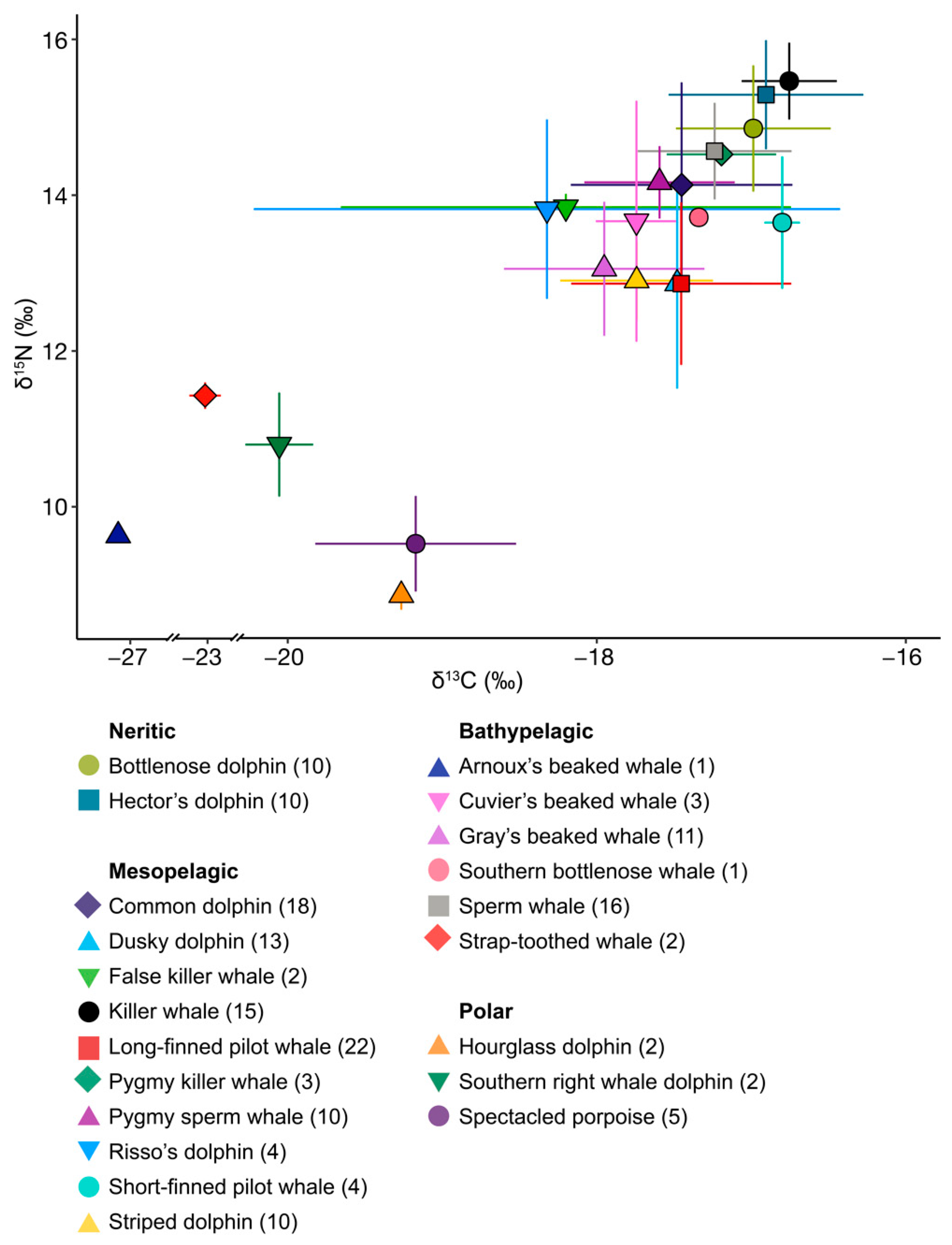
| Group | Species | Latin Name | Preferred Habitat | n | δ13C | δ15N |
|---|---|---|---|---|---|---|
| Neritic | Bottlenose dolphin | Tursiops truncatus | Temperate coastal to pelagic waters [34] | 10 | −16.99 ± 0.50 | 14.83 ± 0.81 |
| Hector’s dolphin | Cephalorhyncus hectori hectori | Coastal waters [35] | 10 | −16.91 ± 0.63 | 15.26 ± 0.70 | |
| Meso- pelagic | Common dolphin | Delphinus delphis | Coastal waters [36] | 18 | −17.45 ± 0.72 | 14.11 ± 1.31 |
| Dusky dolphin | Lagenorhynchus obscurus | Neritic waters above continental shelves [37] | 13 | −17.48 ± 0.48 | 12.84 ± 1.34 | |
| False killer whale | Pseudorca crassidens | Pelagic waters [38] | 2 | −18.20 ± 1.46 | 13.82 ± 0.17 | |
| Killer whale | Orcinus orca | Coastal to offshore, tropical to polar waters [39] | 15 | −16.75 ± 0.31 | 15.43 ± 0.49 | |
| Long-finned pilot whale | Globicephala melas edwardii | Cold temperate oceanic to shelf waters [40] | 22 | −17.45 ± 0.71 | 12.84 ± 1.04 | |
| Pygmy killer whale | Feresa attenuata | Tropical oceanic waters [41] | 3 | −17.19 ± 0.35 | 14.50 ± 0.08 | |
| Pygmy sperm whale | Kogia breviceps | Pelagic waters [42] | 10 | −17.59 ± 0.49 | 14.14 ± 0.46 | |
| Risso’s dolphin | Grampus griseus | Offshore waters [43] | 4 | −18.32 ± 1.90 | 13.80 ± 1.15 | |
| Short-finned pilot whale | G. macrorhynchus | Tropical to warm temperate, oceanic to shelf waters [40] | 4 | −16.8 ± 0.11 | 13.62 ± 0.85 | |
| Striped dolphin | Stenella coeruleoalba | Waters outside the continental shelf, oceanic [44] | 10 | −17.74 ± 0.49 | 12.88 ± 0.51 | |
| Bathy- pelagic | Arnoux’s beaked whale | Berardius arnuxii | Southern hemisphere waters, between 24°S and Antarctica [45] | 1 | −27.16 | 9.63 |
| Cuvier’s beaked whale | Ziphius cavirostris | Oceanic deep waters [46] | 3 | −17.74 ± 0.26 | 13.64 ± 1.54 | |
| Gray’s beaked whale | Mesoplodon grayi | Temperate deep waters [47,48] | 11 | −17.95 ± 0.65 | 13.03 ± 0.86 | |
| Southern bottlenose whale | Hyperoodon planifrons | Deep waters south of 30°S [49] | 1 | −17.34 | 13.69 | |
| Sperm whale | Physeter macrocephalus | Deep waters, tropical to sub-polar [50] | 16 | −17.24 ± 0.50 | 14.54 ± 0.62 | |
| Strap-toothed whale | Mesoplodon layardii | Temperate and subantarctic waters in the Southern Hemisphere [51] | 2 | −23.03 ± 0.16 | 11.42 ± 0.17 | |
| Polar | Hourglass dolphin | L. cruciger | Pelagic-oceanic, polar waters [52] | 2 | −19.27 ± 0.05 | 8.85 ± 0.18 |
| Southern right whale dolphin | Lissodelphis peronii | Circumpolar subantarctic and cool-temperate Southern Ocean waters [53] | 2 | −20.06 ± 0.22 | 10.78 ± 0.66 | |
| Spectacled porpoise | Phocoena dioptrica | Cool temperate, sub-Antarctic, and Antarctic oceanic waters [54] | 5 | −19.17 ± 0.65 | 9.51 ± 0.61 |
| Neritic | Mesopelagic | Bathypelagic | ||||||||
|---|---|---|---|---|---|---|---|---|---|---|
| Species | BD | HD | CD | DD | KW | LPW | PSW | SD | GW | SW |
| BD | ||||||||||
| HD | ||||||||||
| CD | ||||||||||
| DD | ||||||||||
| KW | ||||||||||
| LPW | ||||||||||
| PSW | ||||||||||
| SD | ||||||||||
| GW | ||||||||||
| SW | ||||||||||
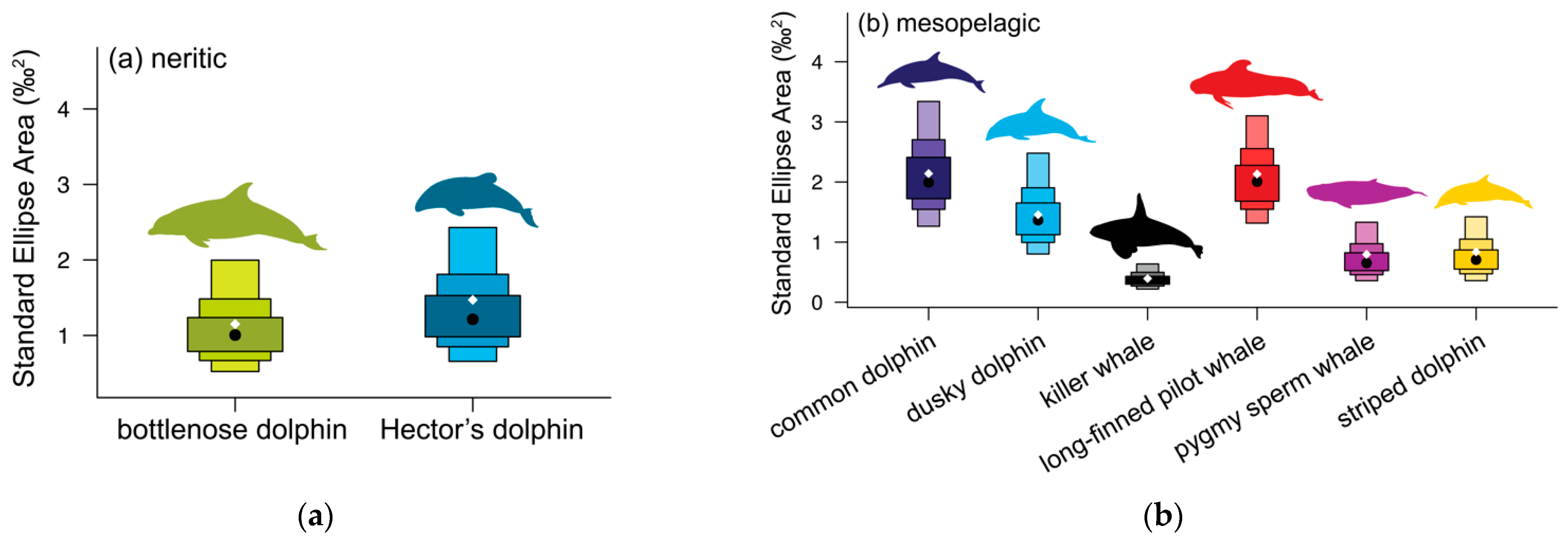
| (a) neritic odontocetes | ||||||
| Metrics | Bottlenose dolphin | Hector’s dolphin | Probability (%) | |||
| N | 10 | 10 | ||||
| SEA | 1.02 | 1.31 | ||||
| SEAC | 1.15 | 1.47 | ||||
| SEAB | 0.78 | 0.99 | ||||
| δ13C range | 1.64 | 1.80 | ||||
| δ13C rangeboot | 1.35 | 1.59 | 76.1% HD > BD | |||
| δ15N range | 2.40 | 2.28 | ||||
| δ15N rangeboot | 2.10 | 1.93 | 64.7% BD > HD | |||
| TA | 1.76 | 2.52 | ||||
| TAboot | 1.82 | 2.01 | 59.1% HD > BD | |||
| CD | 0.84 | 0.85 | ||||
| CDboot | 0.78 | 0.78 | 51.1% BD > HD | |||
| MNND | 0.36 | 0.48 | ||||
| MNNDboot | 0.33 | 0.35 | 56.6% HD > BD | |||
| SDNND | 0.24 | 0.22 | ||||
| SDNNDboot | 0.26 | 0.28 | 56.1% HD > BD | |||
| (b) mesopelagic odontocetes (for probability %, see Table 4) | ||||||
| Metrics | Commondolphin | Dusky dolphin | Killer whale | Long-finned pilot whale | Pygmy sperm whale | Striped dolphin |
| N | 18 | 13 | 15 | 22 | 10 | 10 |
| SEA | 2.01 | 1.33 | 0.37 | 2.03 | 0.71 | 0.74 |
| SEAC | 2.14 | 1.46 | 0.39 | 2.13 | 0.80 | 0.84 |
| SEAB | 2.98 | 1.14 | 2.00 | 2.48 | 2.67 | 1.58 |
| δ13C range | 2.46 | 1.59 | 1.10 | 2.63 | 1.52 | 1.87 |
| δ13C rangeboot | 2.03 | 1.32 | 0.88 | 2.08 | 1.29 | 1.44 |
| δ15N range | 4.83 | 4.53 | 2.14 | 4.64 | 1.37 | 1.75 |
| δ15N rangeboot | 3.63 | 3.68 | 1.46 | 2.93 | 1.21 | 1.33 |
| TA | 5.39 | 2.93 | 0.86 | 6.73 | 1.33 | 1.65 |
| TAboot | 4.66 | 3.06 | 0.74 | 3.54 | 1.03 | 1.10 |
| CD | 1.32 | 1.20 | 0.46 | 1.00 | 0.60 | 0.55 |
| CDboot | 1.24 | 1.14 | 0.45 | 0.98 | 0.56 | 0.53 |
| MNND | 0.45 | 0.47 | 0.20 | 0.45 | 0.36 | 0.39 |
| MNNDboot | 0.60 | 0.48 | 0.23 | 0.53 | 0.25 | 0.26 |
| SDNND | 0.31 | 0.20 | 0.23 | 0.41 | 0.21 | 0.35 |
| SDNNDboot | 0.38 | 0.35 | 0.21 | 0.43 | 0.20 | 0.27 |
| (c) bathypelagic odontocetes | ||||||
| Metrics | Gray’s beaked whale | Sperm whale | Probability (%) | |||
| N | 11 | 16 | ||||
| SEA | 1.35 | 0.58 | ||||
| SEAC | 1.50 | 0.62 | ||||
| SEAB | 1.46 | 1.45 | 98.0% GW > SW | |||
| SEAB overlap | 0.03 | 0.09 | ||||
| δ13C range | 2.35 | 1.62 | ||||
| δ13C rangeboot | 1.81 | 1.43 | 65.7% GW > SW | |||
| δ15N range | 2.51 | 2.50 | ||||
| δ15N rangeboot | 2.33 | 1.81 | 73.7% GW > SW | |||
| TA | 2.98 | 1.51 | ||||
| TAboot | 2.66 | 1.57 | 78.7% GW > SW | |||
| CD | 0.85 | 0.60 | ||||
| CDboot | 0.85 | 0.62 | 86.6% GW > SW | |||
| MNND | 0.49 | 0.24 | ||||
| MNNDboot | 0.36 | 0.31 | 64.1% GW > SW | |||
| SDNND | 0.40 | 0.26 | ||||
| SDNNDboot | 0.34 | 0.27 | 65.4% GW > SW | |||
| Species | BD | HD | CD | DD | KW | LPW | PSW | SD | GW | SW |
|---|---|---|---|---|---|---|---|---|---|---|
| BD | 0.41 | |||||||||
| HD | 0.34 | |||||||||
| CD | 0.19 | 0.50 | 0.27 | 0.22 | 0.11 | |||||
| DD | 0.26 | >0.01 | 0.54 | 0.22 | 0.23 | |||||
| KW | 0.30 | >0.01 | >0.01 | 0.02 | >0.01 | |||||
| LPW | 0.28 | 0.39 | >0.01 | 0.06 | 0.24 | |||||
| PSW | 0.64 | 0.15 | >0.01 | 0.18 | 0.05 | |||||
| SD | 0.31 | 0.42 | >0.01 | 0.63 | 0.04 | |||||
| GW | 0.03 | |||||||||
| SW | 0.09 |
| Species | Metric | CD | DD | KW | LPW | PSW | SD |
|---|---|---|---|---|---|---|---|
| Common dolphin (CD) | SEAB | 84.2 | 100.0 | 54.1 | 99.4 | 99.1 | |
| δ13C range | 94.7 | 99.5 | 44.8 | 95.5 | 85.6 | ||
| δ15N range | 47.5 | 99.5 | 68.4 | 100.0 | 99.9 | ||
| TA | 83.0 | 100.0 | 72.1 | 100.0 | 99.8 | ||
| CD | 63.9 | 100.0 | 79.9 | 1000 | 99.9 | ||
| MNND | 74.1 | 99.3 | 62.5 | 99.2 | 98.2 | ||
| SDNND | 60.1 | 89.9 | 50.4 | 92.8 | 75.2 | ||
| Dusky dolphin (DD) | SEAB | 15.8 | 100.0 | 17.2 | 95.0 | 93.1 | |
| δ13C range | 5.1 | 89.4 | 8.3 | 56.7 | 41.8 | ||
| δ15N range | 52.3 | 99.4 | 67.5 | 100.0 | 99.5 | ||
| TA | 17.0 | 99.6 | 44.7 | 98.8 | 96.3 | ||
| CD | 36.1 | 99.9 | 70.2 | 99.6 | 99.2 | ||
| MNND | 25.9 | 96.8 | 40.9 | 95.1 | 93.0 | ||
| SDNND | 39.9 | 83.2 | 43.1 | 88.0 | 66.5 | ||
| Killer whale (KW) | SEAB | 0.0 | 0.0 | 0.0 | 5.9 | 5.0 | |
| δ13C range | 0.5 | 10.5 | 0.9 | 7.0 | 10.5 | ||
| δ15N range | 0.5 | 0.6 | 13.1 | 62.3 | 57.2 | ||
| TA | 0.0 | 0.4 | 0.6 | 24.6 | 32.0 | ||
| CD | 0.0 | 0.1 | 0.7 | 18.6 | 31.8 | ||
| MNND | 0.7 | 3.2 | 2.7 | 40.6 | 38.1 | ||
| SDNND | 10.1 | 16.8 | 16.7 | 53.0 | 33.5 | ||
| Long-finned pilot whale (LPW) | SEAB | 45.9 | 82.8 | 100.0 | 99.2 | 99.2 | |
| δ13C range | 53.9 | 91.6 | 99.1 | 93.4 | 84.2 | ||
| δ15N range | 31.4 | 32.4 | 86.8 | 97.3 | 93.1 | ||
| TA | 27.9 | 55.3 | 99.4 | 98.4 | 95.7 | ||
| CD | 20.1 | 29.8 | 99.3 | 98.1 | 96.7 | ||
| MNND | 37.5 | 59.1 | 97.3 | 96.7 | 94.6 | ||
| SDNND | 49.6 | 56.9 | 83.3 | 86.5 | 69.4 | ||
| Pygmy sperm whale (PSW) | SEAB | 0.6 | 5.0 | 94.0 | 0.8 | 44.4 | |
| δ13C range | 4.4 | 43.0 | 92.9 | 6.5 | 34.8 | ||
| δ15N range | 0.0 | 0.0 | 35.9 | 2.6 | 33.1 | ||
| TA | 0.0 | 1.2 | 75.4 | 1.6 | 48.5 | ||
| CD | 0.0 | 0.4 | 81.4 | 1.9 | 57.8 | ||
| MNND | 0.8 | 4.9 | 59.4 | 3.3 | 46.8 | ||
| SDNND | 7.2 | 12.0 | 47.0 | 13.5 | 31.2 | ||
| Striped dolphin (SD) | SEAB | 0.9 | 6.9 | 95.0 | 0.9 | 55.6 | |
| δ13C range | 14.4 | 58.1 | 89.3 | 15.8 | 65.2 | ||
| δ15N range | 0.1 | 0.5 | 42.8 | 6.3 | 66.9 | ||
| TA | 0.2 | 3.7 | 68.0 | 4.3 | 51.5 | ||
| CD | 0.1 | 0.8 | 68.2 | 3.3 | 42.2 | ||
| MNND | 1.8 | 7.0 | 61.9 | 5.4 | 53.2 | ||
| SDNND | 24.8 | 33.5 | 66.5 | 30.6 | 68.8 |
Publisher’s Note: MDPI stays neutral with regard to jurisdictional claims in published maps and institutional affiliations. |
© 2022 by the authors. Licensee MDPI, Basel, Switzerland. This article is an open access article distributed under the terms and conditions of the Creative Commons Attribution (CC BY) license (https://creativecommons.org/licenses/by/4.0/).
Share and Cite
Peters, K.J.; Bury, S.J.; Hinton, B.; Betty, E.L.; Casano-Bally, D.; Parra, G.J.; Stockin, K.A. Too Close for Comfort? Isotopic Niche Segregation in New Zealand’s Odontocetes. Biology 2022, 11, 1179. https://doi.org/10.3390/biology11081179
Peters KJ, Bury SJ, Hinton B, Betty EL, Casano-Bally D, Parra GJ, Stockin KA. Too Close for Comfort? Isotopic Niche Segregation in New Zealand’s Odontocetes. Biology. 2022; 11(8):1179. https://doi.org/10.3390/biology11081179
Chicago/Turabian StylePeters, Katharina J., Sarah J. Bury, Bethany Hinton, Emma L. Betty, Déborah Casano-Bally, Guido J. Parra, and Karen A. Stockin. 2022. "Too Close for Comfort? Isotopic Niche Segregation in New Zealand’s Odontocetes" Biology 11, no. 8: 1179. https://doi.org/10.3390/biology11081179