Article

Resolving Selected Problems in Surface Topography Analysis by Application of the Autocorrelation Function

by
Przemysław Podulka
Faculty of Mechanical Engineering and Aeronautics, Rzeszow University of Technology, Powstancow Warszawy 8 Street, 35-959 Rzeszów, Poland
Coatings 2023, 13(1), 74; https://doi.org/10.3390/coatings13010074
Submission received: 30 November 2022 / Revised: 27 December 2022 / Accepted: 29 December 2022 / Published: 31 December 2022

Abstract

:
In this paper, the validity of the application of an autocorrelation function for resolving some surface topography measurement problems was presented. Various types of surfaces were considered: plateau-honed, honed with burnished dimples, ground, turned, milled, laser-textured, or isotropic. They were measured with stylus and non-contact (optical) methods. Extraction of selected features, such as form and waviness (defined as an L-surface) and high-frequency measurement noise (S-surface) from raw measured data, was supported with an autocorrelation function. It was proposed to select the analysis procedures with an application of the autocorrelation function for both profile (2D) and areal (3D) analysis. Moreover, applications of various types of regular (available in the commercial software) analysis methods, such as least-square-fitted polynomial planes, selected Gaussian (regression and robust) functions, median filter, spline approach, and fast Fourier transform scheme, were proposed for the evaluation of surface topography parameters from ISO 25178 standards.

1. Introduction

Analysis of surface topography, which is obtained in the final stage of treatment, can be crucial in many functional applications [1]. The measurement and studies of surface properties, such as wear resistance [2], sealing [3,4], friction [5], lubricant retention [6], energy consumption [7] or eco-friendly factors [8], and many more [9,10,11], in general, can be received from the description of surface topography. Moreover, in some cases, it is defined as a fingerprint of the manufacturing process [12], especially that can be absolutely essential in the process of control [13].
Considering all of the mentioned and further additional issues, analyzing surface topography can be an encouraging task to be resolved. The whole process of results evaluation can be, even roughly, divided into various, however dependent, sub-processes. Firstly, an appropriate measurement method must be proposed to receive relevant results. Generally, those methods can be divided into stylus [14], proposed with many traditional systems [15], and non-stylus techniques [16], where the optical methods have many advantages [17]. They (stylus and optical techniques) were widely compared in many previous studies [18,19,20]; nevertheless, the most particularly noticeable improvement was in reducing the time of measurement [21].
Very popular and, respectively, often applied in surface topography analysis are methods with the application of the autocorrelation function (ACF) exhibit possible various, e.g., random and periodic, features buried on the machined surface [22]. Math basics of ACF were presented in [23]. Moreover, the roughness amplitudes with the non-random distribution can be thoroughly evaluated by the ACF method [24]. This function can be used when the accurate prediction of the machined surface topography of abrasive belt flexible grinding is required [25]. Moreover, ACF provides two-point correlated information about the spatial relation and dependence of data, indicating randomness or periodicity and isotropy or anisotropy of surface features can be received with this application [26]. Generally, the surface texture orientation can be properly evaluated as well [27]. Different ACF in combination with statistical parameters can be generated and then compared with the prescribed ground surfaces [28]. In addition, feature extraction can be significantly improved with the function presented [29].
Analyzing image data, e.g., fractal analysis on the surface topography image of thin films [30] can be supported by many advantages of ACF applications, compared with many other approaches [31]. Roughness received by the scanning tunneling microscope (STM) measurement can be represented by the ACF [32]. This method was widely used for plateau-honed [33] or polished [34] topographies for an efficient grain size determination. Generally, surface roughness can be characterized by the widths of ACFs, which can be obtained from the digital processing of surface images [35]. The properties of the ACF can be extremely advantageous, e.g., bi-directionality in the soil surface roughness investigation [36].
Except for the characterization of surface topography, the ACF is often proposed in the process of data generation, e.g., for analyzing mixed lubrication [37]. Furthermore, when investigating the precision of generation, correlation distances can be calculated from the ACF of the generated data [38]. Identification and reconstruction of Bi-Gaussian surfaces can be received with ACF characterization [39]. This is an important function to describe surface roughness and depends on the nature of morphology and, respectively, the powers spectrum can be evaluated from the ACF [40] as well. The function describes the general dependence of the values of the data at one position on the values at another position or, correspondingly, the ACF is used for surface topographic assessment to indicate the randomness and directionality of surface features [41], described as the theoretical directional variogram [42] in some cases.
The advantages of the application of ACF were presented widely, nevertheless, its suitability in the definition of the S-surface (reducing the high-frequency measurement noise) and L-surface (an areal form removal) was not comprehensively studied. The L-surface (S-surface) is obtained by the application of the L-filter (S-filter), a filter eliminating the largest (the smallest) scale elements from the surface [43]. Some of the results presented for a profile (2D) and an areal (3D) roughness evaluation [44] indicated its suitability in the detection of high-frequency errors [45] when describing the S-surface, however, its validation must be improved.
Errors in roughness evaluation can be received from various sources. Firstly, the measuring method can influence the reliability of the results obtained. Optical methods are fast, compared to that stylus [46], nevertheless are fraught with many errors that can radically affect the results of surface topography analysis. One of the types of errors is those in the high-frequency domain. High-frequency measurement noise is a type of noise that can be caused by instability of the mechanics with any influences from the environment or, on the other hand, by internal electrical noise [47,48]. However, in most cases, the high-frequency noise is a result of vibration [49,50].
Considering the analysis of machined parts, such as cylindrical elements of the engine, the surface roughness parameters are calculated after an areal form removal. From that matter, even if both an appropriate and precise measurement technique (device) is applied, properties of the surface can be described erroneously when the data processing is not selected carefully. Considering all of the sophisticated methods, there are many algorithms and, respectively, procedures for the reduction of errors in data processing, their selection requires mindful users [51].
When defining the L-surface, distortions of the results can be found for the areas where deep or wide features are located [52,53]. There were many studies performed for form extraction, taking into consideration the location of the features, especially in the edge area of the analyzed detail [54]. Some modifications of the commonly used in surface characterization, the Gaussian filtration method, can be an alternative solution [55]. The enlargement of dimple distortion was found when features were located near/on the edge of considered data [56]. Much crucial information can be received with a profile exploration [57] that, respectively, in some cases, 2D characterization can allow defining more confidential results than 3D studies [58,59]. From that matter, the effect of feature size, distribution, and density was considered for the definition of the L-surface with an application of general, available in the commercial software, methods [60].
In this paper, the ACF method was applied for validation of methods for an areal form removal and definition of the high-frequency measurement errors. Both surfaces, S-surface and L-surface, can be more precisely obtained when a comprehensive analysis of the ACF is applied. Many advantages of this method were presented in the analysis of the Gaussian surfaces [61,62,63]. Moreover, the main proposal of the studies presented was to indicate both the usefulness and suitability of the ACF application, proposing its usage with other, also available in the commercial software, function, such as a power spectral density (PSD) [64,65,66,67,68] or thresholding [69,70] methods. The usage of ACF in the definition of the L-surface was not comprehensively studied in previous research. Moreover, many advantages in the calculation of the S-surface (for high-frequency measurement noise reduction) with ACF application must be highlighted as well. It was proposed to validate the methods of definition of L-surface and S-surface with an application of ACF. It was found that the precision of the S-L surface definition can be significantly improved with ACF usage. Errors in the calculation of ISO 25178 surface roughness parameters can be also reduced when the ACF function was applied.

2. Materials and Methods

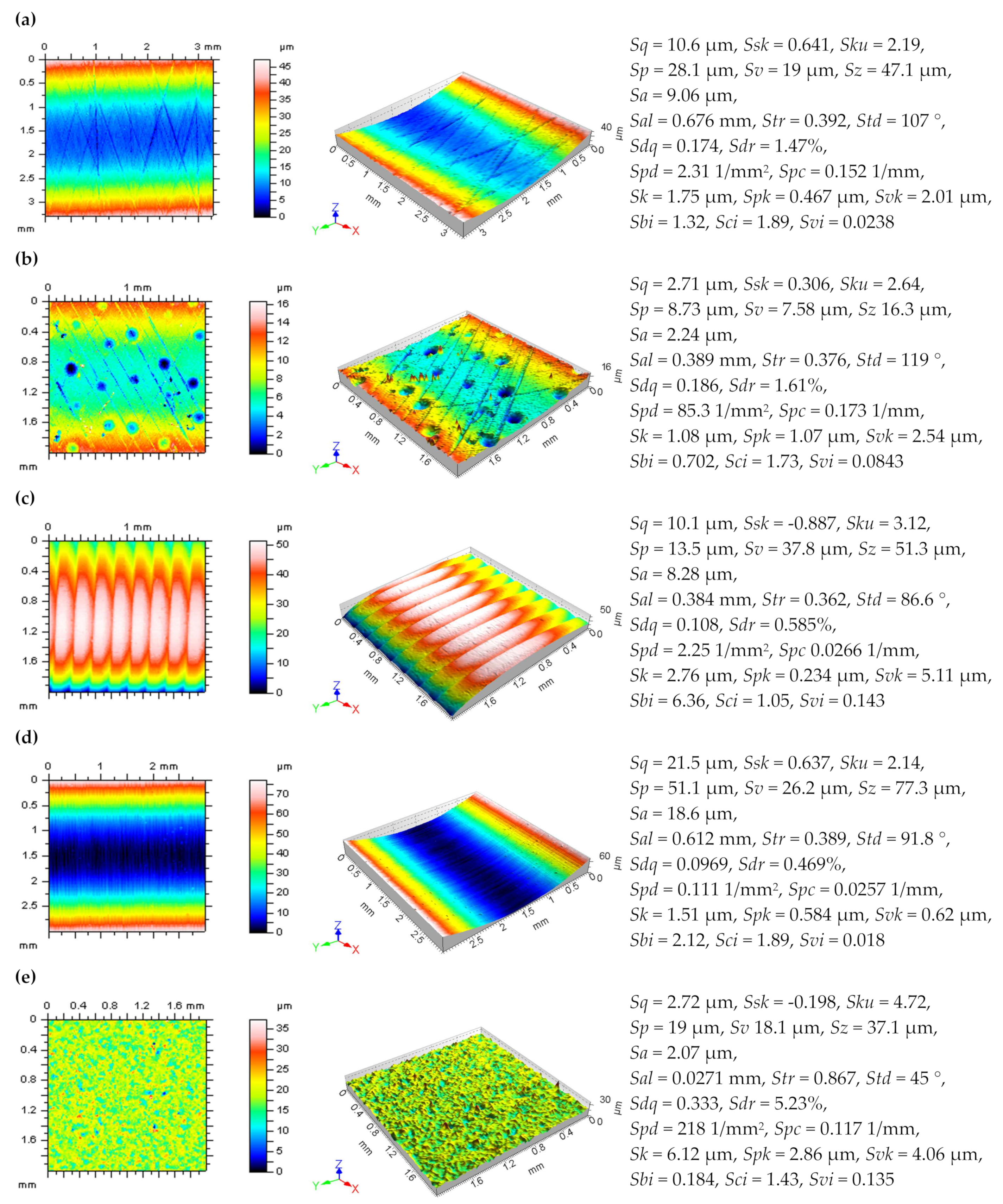
2.1. Analyzed Surfaces

Various types of surface topographies were considered: plateau-honed, with a cross-hatch pattern equal to 60°, some of them with additionally burnished oil pockets (dimple’s average width and average depth were around 0.2 mm and 10 μm, respectively, and the area density of oil pockets was smaller than 20%), turned, ground, and isotropic details. More than 20 measured surfaces of each type were considered to provide some repeatability in the analysis of the results but only a few of them were presented in detail.
In Figure 1, contour map plots (left column), isometric views (middle), and selected ISO 25178 surface topography parameters including some from the Sk family (right column) were presented for each of the types of surfaces. Both types of plateau-honed cylinder liners (Figure 1a,b), turned (Figure 1c) and ground (Figure 1d) details were presented as raw measured data, containing the form, cylindrical shape, and waviness, if existed. For this type of data, both L-surfaces and, respectively, S-surfaces were defined with the ACF improvement. An example of an isotropic surface (Figure 1e) was flat, respectively, an areal form removal process, described as a definition of the L-surface, was not considered in the studies presented. For this type of surface, the ACF method was applied to detect and reduce the effect of the high-frequency errors, obtained as an S-surface, from the results of the measurement process, namely the raw measured data.
The values of the following, located in the ISO 25178 standard [71,72], surface topography parameters were measured, calculated and considered: root mean square height Sq, skewness Ssk, kurtosis Sku, maximum peak height Sp, maximum valley depth Sv, the maximum height of surface Sz and arithmetic mean height Sa from the height parameters; autocorrelation length Sal, texture parameter Str, and texture direction Std from spatial parameters; root mean square gradient Sdq and developed interfacial areal ratio Sdr from hybrid parameters; peak density Spd and arithmetic mean peak curvature Spc from feature parameters; core roughness depth Sk, reduced summit height Spk, reduced valley depth Svk, upper material ratio Sr1, and lower material ratio Sr2 from functional parameters; surface bearing index Sbi, core fluid retention index Sci and valley fluid retention index Svi from the functional indices [73].

2.2. Measurement Process

Analyzed details were measured with different stylus or non-contact (optical) techniques. The Talyscan 150 and Talysurf CCI Lite (produced by Taylor Hobson Ltd, Leicester, U.K., version 2.8.2.95) devices were applied as the stylus and optical measuring equipment, respectively.
For the stylus instrument: a nominal tip radius of 2 μm, height resolution of 10 nm and the measured area 5 by 5 mm with 1000 × 1000 measured points, were applied. The sampling interval was equal to 5 μm. The measurement speed was 0.75 mm/s. The effect of the measurement velocity was not studied, it was not the subject of the current research but, respectively, was analyzed in the previous studies.
For the non-contact measurement: the height resolution was 0.01 nm, and the measured area was 3.35 by 3.35 mm with the 1024 × 1024 measured points, respectively, obtained. The spacing was 3.27 μm. A Nikon 5×/0.13 TI objective (Nikon GmbH, Düsseldorf, Germany) was used.
In the study presented for both methods, the effect of sampling (stylus) and spacing (non-contact) on the values of 3D surface roughness parameters were not considered.
For both analyses, TalyMap Gold software (version 6.1), copyrighted by Digital Surf (Besançon, France), was used for digital filtering and ISO 25178 surface topography parameters calculation and, respectively, evaluation.
All the surfaces measured by the non-stylus device were carefully studied for the detection of the individual peaks [74] (spikes [75]) errors from the raw measured data. This type of error was observed for the optical measurement technique. Individual peaks were reduced by the thresholding method with a selected material ratio from 0.13% to 99.87% [76].

2.3. Proposals of Improvement of Methods for Surface Topography Analysis by Application of the Autocorrelation Function

Evaluation of surface roughness was provided after an areal form removal (definition of an L-surface) and reduction of high-frequency measurement noise (proposals of an S-surface). For the definition of the L-surface and S-surface, the following methods were proposed: least-squares fitted cylinder (LSFC), the least-square fitted polynomial of 2nd degree (Poly2), regular Gaussian regression filter (GRF), robust Gaussian regression filter (RGRF), regular isotropic spline filter (SF), median denoising filter (MDF) and fast Fourier transform filter (FFTF). All of those methods are available in commercial software (version 6.1). For improvement of the proposed procedures, the following data analysis techniques were additionally used: the autocorrelation function (ACF) and power spectral density (PSD) were received from these sources as well.
The least-square fitting (LSF) is an often-used method for surface roughness evaluation. Considering the ISO 13565-3 standard [77], the LSF method was applied directly for the running-in-wear process analysis of the plateau surface [17]. Furthermore, the LSF method is proposed when defining the ISO 21920–2 parameters needed for evaluating the roughness of plateau structure surfaces [78]. The reference planes defined in this study by L-surface for assessing nominally flat and curved surfaces were recommended with LSF methods [79]. Based on the LSF method and the electrostatic field theory, the linear relationship between the work function (WF) and the surface roughness of the alloys [80] can be found. LSF can be applied in both shapes (cylinder [81]) and polynomial [53] when the definition of the reference plane. Machines such as the coordinate measuring machine (CMM) often employ the LSF algorithms [82]. Furthermore, the LSF approach can be used to calibrate the profile least-square median of the surface texture curve [83].
Widely proposed and, respectively, applied are filters based on the Gaussian function [84]. One of the most commonly used is a regular Gaussian filter (GRF) [85]. Many types of surfaces can be characterized by the Gaussian filters, and apart from many tribological studies, the roughness of granular materials can be evaluated as well [86]. Often proposed modification of the regular Gaussian filter is a robust scheme [87]. The robust Gaussian regression filter (RGRF) has been proposed in many surface characterization problems, including the surface topography analysis of ultra-precision machined surfaces [88].
An alternative to many non-resolved problems with Gaussian filtering methods is a spline. The universal spline filter, combined with the FFT algorithm, can reduce the computation time considerably [89]. When separating the roughness, waviness, and form, the variational problem can be solved by approximating the filtered surface data employing different two-dimensional functions, e.g., B-spline [90]. Nevertheless, compared to the Gaussian methods (e.g., GRF), the spline filter (SF) was often found that generate more errors [91].
Digital data processing, especially of image sources, is often proposed with median filters [92]. The application of a median filter can be valuable in the preprocessing unit that corrects surrounding light levels and filters noise [93]. The median denoising filter (MDF) can be especially valuable in the elimination of the bad points that, respectively, a 3 × 3 denoising filter is proposed as a spatial operator [94].
As an alternative for ACF characterization, it was provided that PSD can be valuable in the correct determination of surface morphology when scanning force microscopy (SFM) [95] or atomic force microscopy (AFM) [96] imaging analysis of the surface roughness was presented. It is found, additionally, that if PSD roughness is expressed as a polynomial function, the international roughness index (IRI) can be simply calculated [97]. A similar variation of low-frequency roughness of swift heavy ion (SHI) irradiated ultra-thin gold films can be received with PSD application [98]. Fourier techniques, which are the basics of PSD analysis, can characterize the wavefront of optical components in various directions [99]. An angular spectrum, derived from the PSD, can be often employed to research the spatial distribution of spectral energy for the milled surface [100]. The effects of feed and vibrations on surface roughness can be researched with the use of PSD as well [101]. Furthermore, various measuring instruments can be compared for roughness evaluation by using the PSD functions [102]. Comparing, respectively, the fast Fourier transform (FFT) plots and angular spectrum of different types of wear particles can be demonstrated with calculated PSD function [103]. As already mentioned, isotropy and anisotropy [104]. The PSD was proposed to analyze surface roughness profiles in single-point diamond turning [105]. Generally, the profile (2D) PSD advantages were clearly presented previously [106]. Finally, the PSD, considering both profile (2D) and an areal (3D) roughness evaluation, was entirely beneficial in the process of high-frequency measurement error reduction from the raw measured data [44,45,47,58].

3. Results

This section is divided into three parts. Firstly, in Section 3.1., the ACF was applied for improvements of the methods for an areal form removal (definition of L-surface). Secondly, in Section 3.2, the application of ACF in the definition and reduction of high-frequency measurement noise was presented. Moreover, in the end, in Section 3.3, analysis of modeled data was introduced for improving the ACF methods proposed.

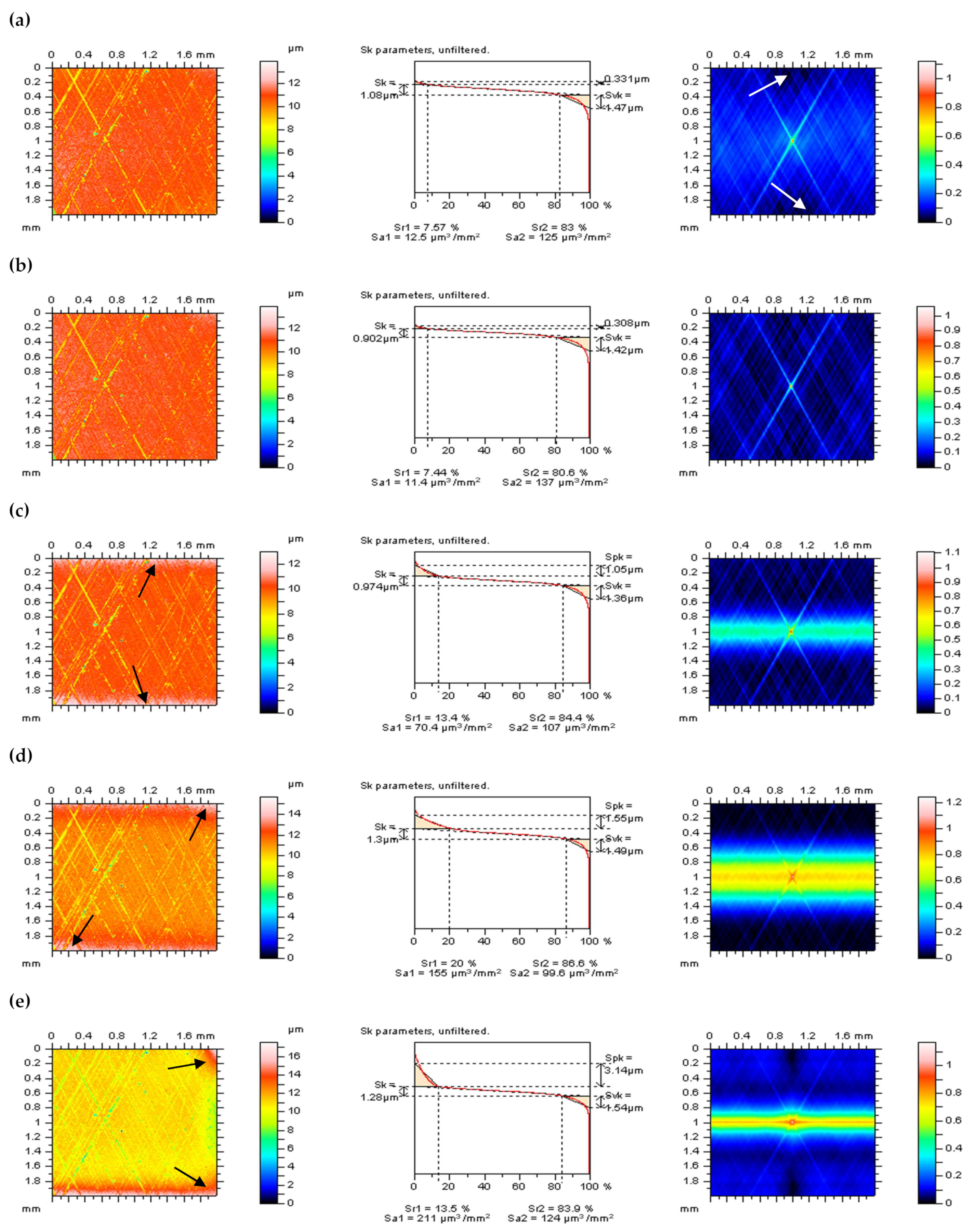
3.1. Reducing Errors in an Areal Form Removal

It was found that the detection of errors in the definition of L-surface can be validated by the ACF. In Figure 2, a 3D ACF (right column) was presented for the plateau-honed cylinder liner surface after an areal form removal by various methods. From the view of both isometric surfaces (left column) and 3D ACF, it was found that if the form (shape and waviness) were not entirely removed, it was indicated by arrows. From that matter and, respectively, by minimization of the values of Sk and Spk parameters [107], the reference plane received by the Poly2 seems to be the best solution from those considered. In Figure 3, extraction of the free-of-dimple method [108] was proposed for validation of an areal form removal approach for plateau-honed cylinder liner surfaces containing additionally burnished oil pockets. Considering both the extracted details (Figure 3c) and its ACF (Figure 3e), the Poly2 seems to provide more encouraging results than GRF and SF schemes.

3.2. Application of an Autocorrelation Function in the Reduction of High-frequency Measurement Errors

When defining an appropriate method for high-frequency measurement noise detection and suppression, the noise surface (NS) [33] was defined. The NS is obtained as the surface created by high-frequency errors. In this case, it is the result of S-filtering. In Figure 4 (right column) were presented NSs created by five various filtering methods of turned piston skirt surface. When analyzing the isometric view of NS, it can be found that some of them contain features that are not located in the high-frequency domain, such as after the application of RGRF or MDF methods (Figure 4b,d). It can indicate that NSs do not contain only high-frequency components. It was found that removal other than noise features from the raw measured data can affect the distortion of surface roughness [12]. Some features can be distorted, such as dimples, oil pockets, holes, scratches, and surface treatment traces in general. This, correspondingly, can significantly affect the values of surface roughness parameters. The more non-noise features are found on the NS, the more distortion in roughness evaluation can be obtained.
From all of the analyzed methods (GRF, RGRF, SF, MDF, and FFTF), considering studies of an isometric view of the S-surface (NS), the application of GRF, SF, and FFTF seem to be particularly suitable; they did not contain non-noise features. To confirm this supposition, an analysis of an areal ACF can be employed. It was found that ACF can be applied for the detection [109] or identification [39] of some surface topography features, especially when various surface textures are considered with fractional approaches [110]. From that matter, in Figure 5, an areal ACFs were presented (left column) for each of the applied filtering procedures. Usage of ACF improved that NS received by RGRF and MDF application caused the removal of non-noise features from the raw data.
Nevertheless, for the GRF scheme, the non-noise features were also defined (Figure 5a) when there were not clearly visible while analyzing the isometric view of the NS. This issue was improved with the thresholding method. The ACF was thresholded with a range equal to 0.13%–99.87% value. This value of thresholding, representing the data truncation, was studied previously [69]. Additionally, for the random surface with Gaussian ordinate distribution height, the difference between material ratios (0.13%–99.87%) was defined as equal to 6 standard deviations of surface amplitude [76]. However, the effect of the thresholding range was not studied in this paper. The accuracy was not considered as it was for the non-noise features indicated.
The occurrence of non-noise features was easily detectable when a thresholded ACF was considered. For results obtained after GRF, RGRF, and MDF application, the non-noise features were found. Contrary to those methods, the usage of SF and FFTF did not define the non-noise features on their NSs (Figure 5c,e). From that procedure, the SF and FFTF approaches seem to cause the smallest errors in the process of high-frequency measurement noise reduction from the raw measured data of turned piston skirt surfaces.
Furthermore, the ACF method was found suitable for both the definition and reduction of high-frequency measurement noise [12,47,58] with profile (2D) and areal (3D) improvements [44]. In Figure 5, additionally, selected profiles (right column) extracted from an areal thresholded ACFs (middle column) were presented. According to the profile characterization, some distortion of the shape of the function was found for the ACF defined with an FFTF method; it was indicated by the arrow in Figure 5e. This exaggeration was found in an areal ACF as well in the center part of the function. The influence of the shape and its distortion, respectively, of the center part of the ACF, was comprehensively studied previously [47], and it was found that its properties can indicate the occurrence of high-frequency measurement errors. In the considered case, it can indicate if the received data still contain noise components.
From the ACF improvement, it can be both validated, firstly, if NS contains non-noise features and, respectively, secondly, if noise data are included in the received surface for which the roughness parameters are calculated.

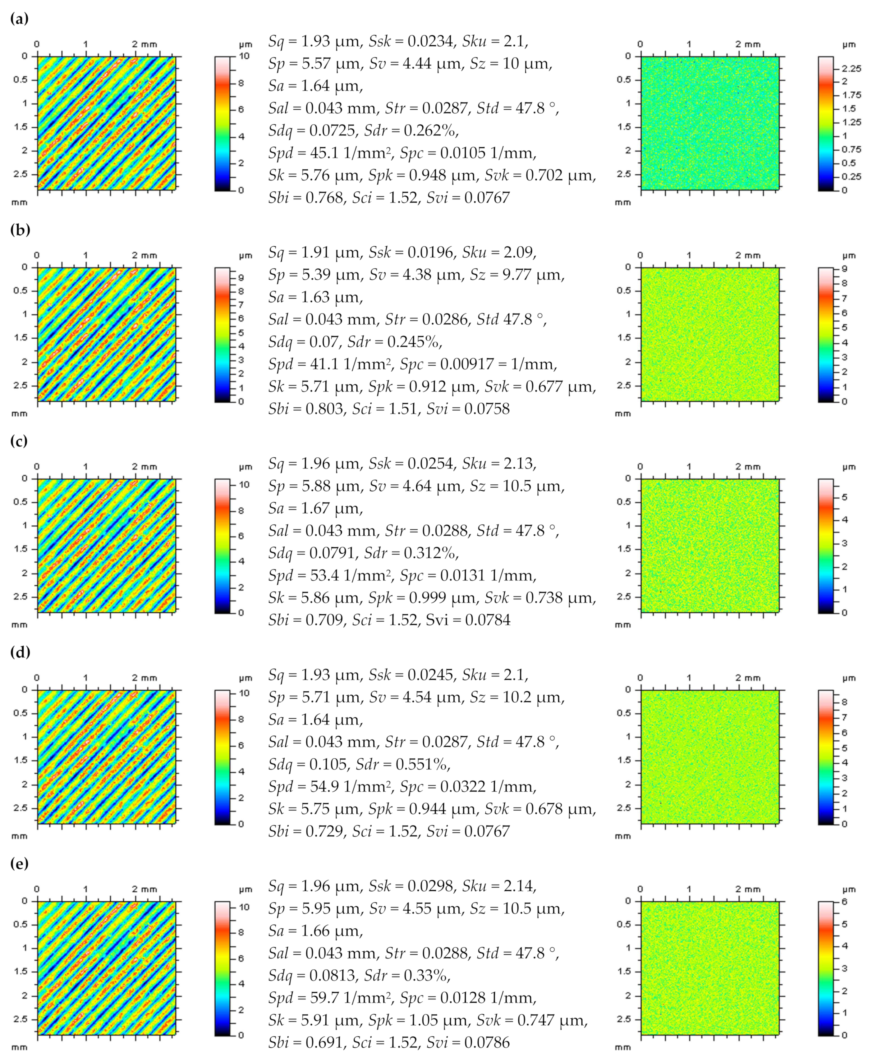
3.3. Improving Proposed Methods with a Modeled Data

For improvement and validation of the results received, surfaces with modeled form (selected L-surfaces) and high-frequency errors (S-surfaces) were considered. Furthermore, both modeled data were then removed by application of various commonly used and available commercial software methods mentioned previously. For an areal form removal, it was improved that least-square fittings of the polynomial plane of 2nd degree (Poly2) caused less distortion of the surface features than various (Gaussian, spline, median or fast Fourier transform) filtering techniques. Moreover, the distortion of modeled surface features was enlarged when they were located near/on the edge of the analyzed detail. Differences in surfaces containing high-frequency noise can be seen in the surface contour map plots (Figure 6a,e). A similar conclusion can be found for profile characteristics. When considering the 3D ACF, differences were difficult to be resolved; nevertheless, some modifications of the center (maximum) value of this function can be resolved. The center part of the ACF was distorted when containing the noise (Figure 6c,g). It was also found that increases in the amplitude of the high-frequency noise caused an enlargement of the distortion of the center part of the ACF [47]. It was also found that properly defined NS should be isotropic. From that matter, its ACF should also exhibit isotropic characteristics. When applying SF and FFTF, it was found that both NS and ACF received the most isotropic properties. From that issue, both mentioned filtering methods can be classified as especially suitable for the suppression of high-frequency noise from the results of surface topography measurements.

4. Conclusions

Based on the results presented, the following conclusions can be raised:
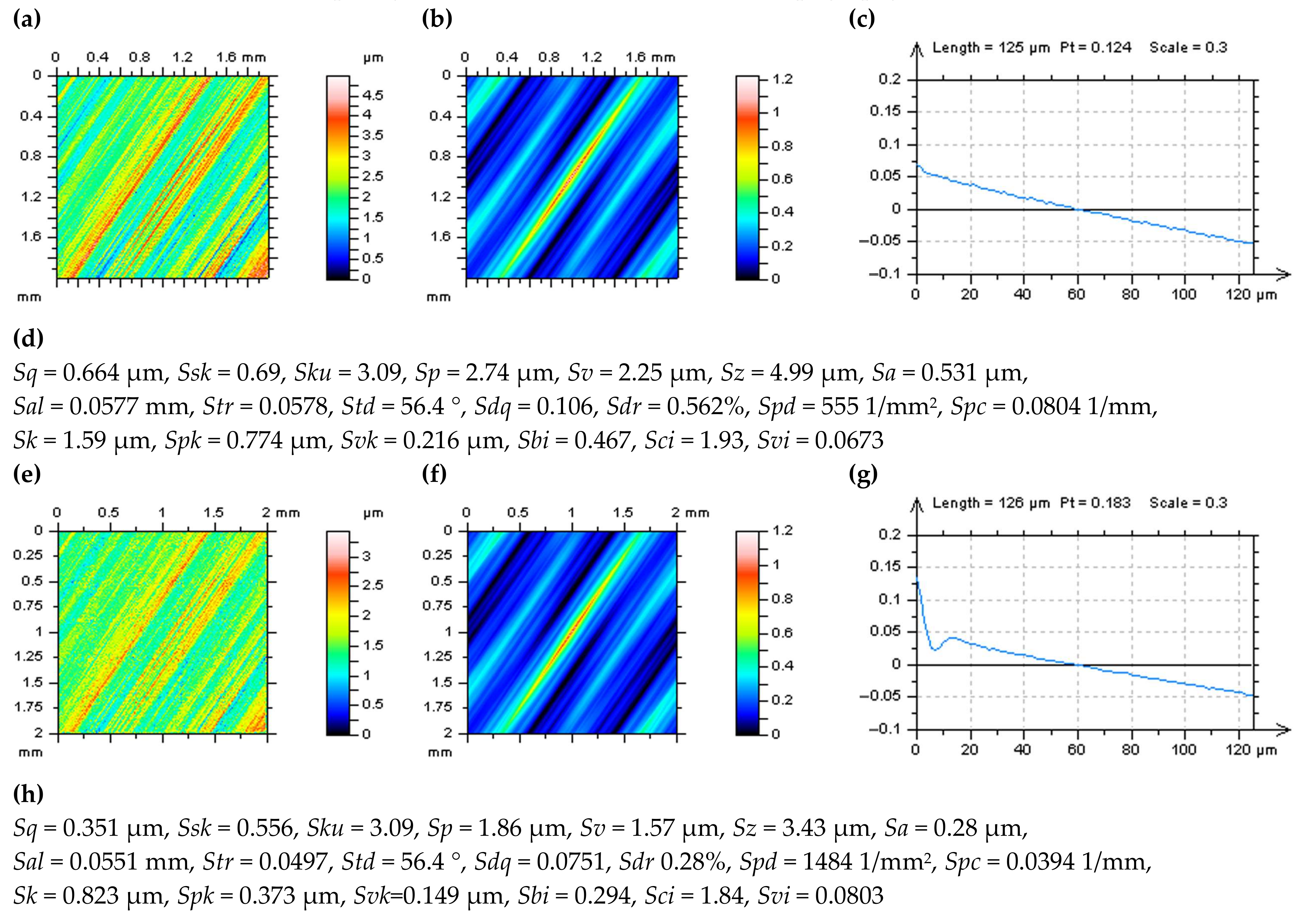
  • The autocorrelation function (ACF) can be exceedingly valuable in the validation of the methods for an areal form removal (definition of L-surface). It was presented that using an ACF with analysis of an isometric view of the measured surface topography can improve the applied method and can be crucial in the reduction of errors in ISO 25178 standard amplitude (height) parameter calculation.
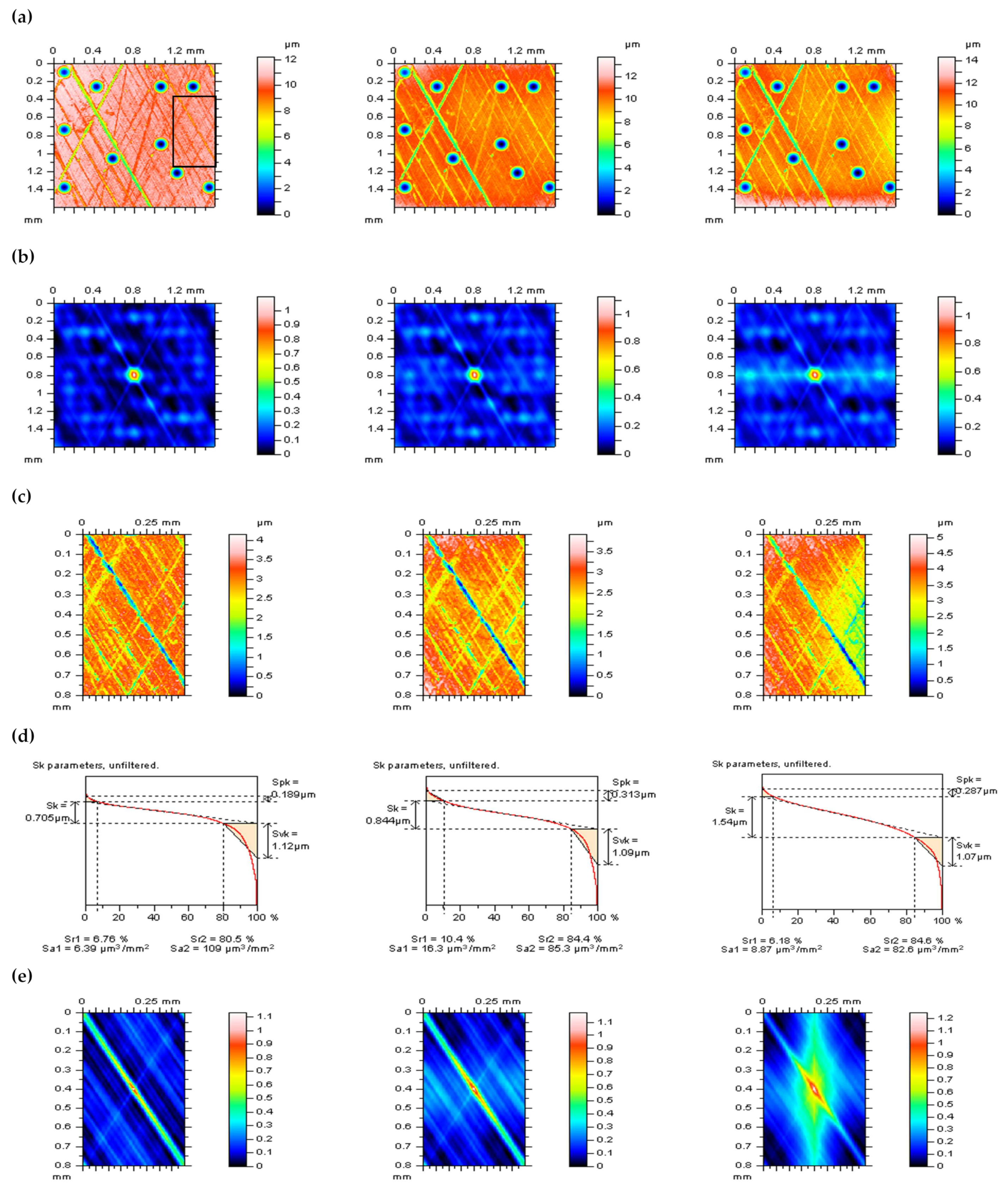
  • When considering the isometric view of the detail after L-surface removal, the distortion of some features (such as burnished dimples) can be important in both measured data and an areal ACF characterization. The higher distortion of data occurs, the greater differences in the isometric view and ACF were obtained. Reduction of errors in both data can, respectively, similarly reduce the distortion in the ISO 25178 roughness parameters calculations.
  • The usage of ACF for details with out-of-feature characteristics can be highly beneficial when the surface contains some deep or wide features, such as dimples. In these cases, omitting the deep features can be necessary for ACF implementation that can affect proposed procedures to be useless. For both analyses, view of surface and ACF graphs, omitting the features is crucial for the definition of S-L-surface.
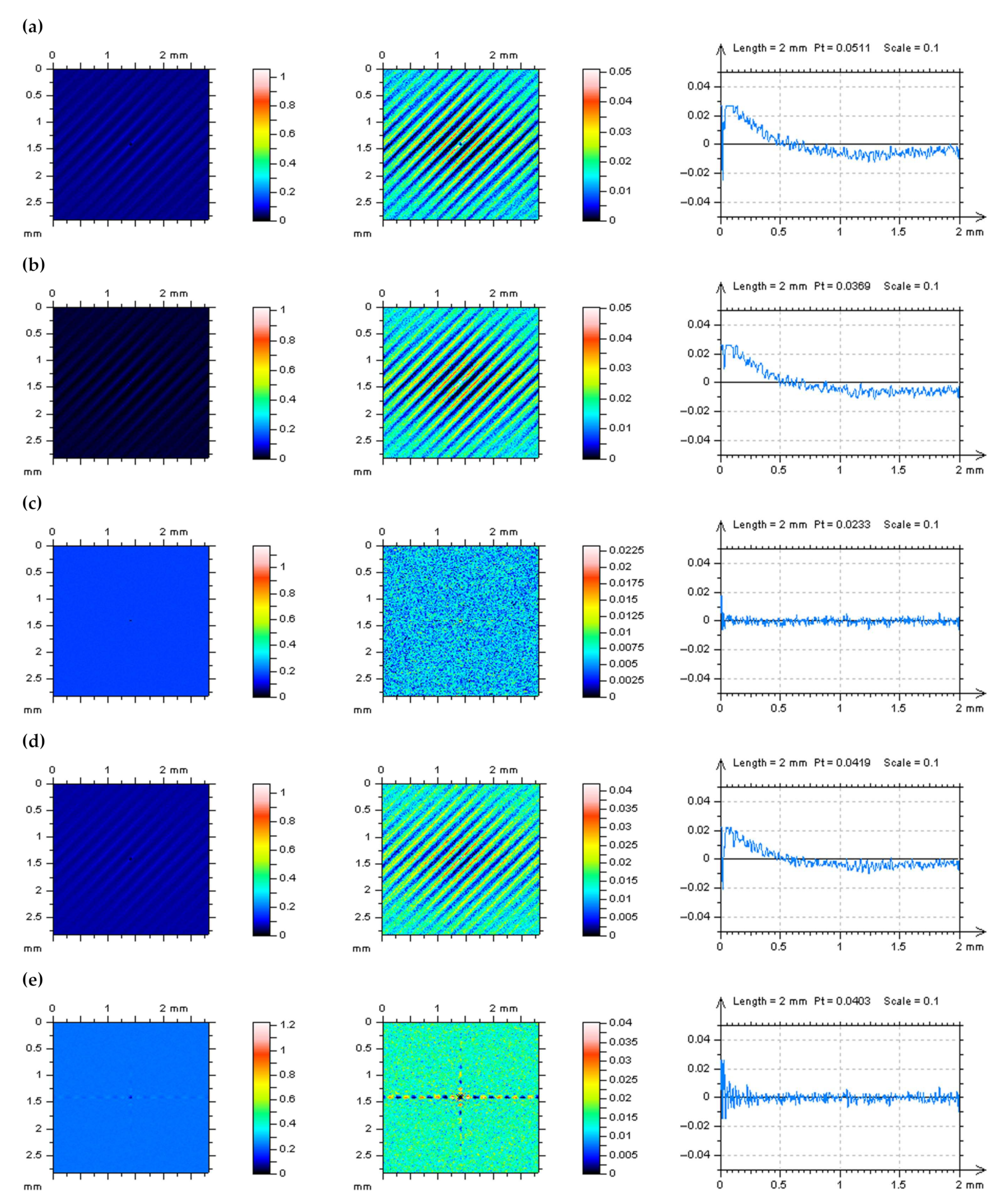
  • Application of ACF for both profile (2D) and an areal (3D) data can be essential in the process of detection (definition) and reduction (removal) of high-frequency measurement errors from the results of surface roughness evaluation. For both types of data analysis, the center part of the ACF can characterize if the measurement errors in the high-frequency domain were reduced entirely. From that matter, filtering method suitability can also be evaluated.
  • In some cases, the thresholding of the ACF is required. This technique is significant in the definition of S-surface especially. When applying truncation, some required properties of the S-surface (noise surface) can be defined more adequately. This approach, supporting the ACF characterization, can reduce the distortion of surface topography features, so, respectively, the errors in the calculation of the ISO 25178 surface roughness parameters can also be radically reduced.
  • Considering thresholding and out-of-feature methods, they can be applied simultaneously when reducing surface height is crucial in the validation of the filtering technique. The sequence of application of those methods does not affect the analyzed type of surface, but, respectively, the sizes, densities, and distribution of the features located on the studied surface must be thoroughly considered.
  • From all of the studies provided, it was presented that the application of the ACF scheme can significantly reduce the errors in the processes of an areal form removal (definition of L-surface) and suppression of high-frequency measurement noise (indicated as the S-surface). It was proved that even regular and commonly used methods can be especially valuable when applied appropriately.
  • All of those data processing actions are crucial in the process of control of manufactured parts. Reducing errors in surface roughness measurement and data analysis can radically affect the validation of machined parts. Improper definition of S-L surface, especially L-surface, can cause classification of properly made parts as a lack and its rejection. From that matter, all of the actions made on the reduction of errors in roughness evaluation (definition of S-L surface) can be consequently crucial in industrial applications.

5. The Outlook

Despite many issues proposed, there can still be some problems not entirely resolved, as follows:
  • Comprehensive analysis of the ACF for both 3D (areal) and 2D (profile) data must be improved in the edge effect of surface filtering. Many studies provide some general proposals for reducing the effect of edge data on the surface roughness evaluation; nevertheless, the reduction of errors in ISO 25178 parameters calculation with the usage of ACF was not already presented.
  • Even though least-square methods, such as least-square fitted cylinder elements or polynomial planes of various degrees, are providing encouraging results, digital filtering, e.g., those based on the Gaussian function, is still often used and the results considered. From that matter, more studies on the Gaussian filtering methods must still be proposed.
  • In some cases of analysis with ACF function, the thresholding method is required. Even though a range (0.13%–99.97%) of thresholding techniques was proposed, according to the previously studied cases, those values should be studied considering each type of surface texture. Moreover, the dependences on the surface feature size, density, and location can also be found when the thresholding method is used.
  • The influence of surface directionality on the ACF characterization should be studied as well. It was introduced in some previous studies that direction methods can be exceedingly valuable in the process of high-frequency measurement noise reduction, improving its impact in both the detection and removal of noise data.
  • The effect of the bi-directionality of surface features was not comprehensively studied in both L-surface and S-surface definitions. When reducing errors in high-frequency measurement noise reduction, the S-surface properties were studied when one or even two directions were defined on the analyzed surface. It must be studied widely, and, respectively, some proposals should be unified.

Funding

This research received no external funding.

Institutional Review Board Statement

Not applicable.

Informed Consent Statement

Not applicable.

Data Availability Statement

Data sharing is not applicable to this article.

Conflicts of Interest

The author declares no conflict of interest.

Nomenclature

The following abbreviations and surface roughness parameters are used in the manuscript:
ACF autocorrelation function
AFM atomic force microscopy
CMM coordinate measuring machine
FFT fast Fourier transform
FFTF fast Fourier transform filter
GRF Gaussian regression filter
IRI international roughness index
L-surface long-wavelength surface
LSFC least-square fitted cylinder shape
LSF least-square fitting method
MDF median denoising filter
NS noise surface
Poly2 least-square fitted polynomial plane of 2nd degree
PSD power spectral density
RGRF robust Gaussian regression filter
S-surface short-wavelength noise surface
SF spline filter
SFM scanning force microscopy
SHI swift heavy ion
STM scanning tunneling microscope
Sa arithmetic mean height Sa, µm
Sal autocorrelation length, mm
Sbi surface bearing index
Sci core fluid retention index
Sdq root mean square gradient
Sdr developed interfacial areal ratio, %
Sk core roughness depth, µm
Sku kurtosis
Sp maximum peak height, µm
Spc arithmetic mean peak curvature, 1/mm
Spd peak density, 1/mm2
Spk reduced summit height, µm
Sq root mean square height, µm
Sr1 upper material ratio
Sr2 lower material ratio
Ssk skewness
Std texture direction, °
Str texture parameter
Sv maximum valley depth, µm
Svi valley fluid retention index
Svk reduced valley depth, µm
Sz the maximum height of surface, µm

References

  1. Panjan, P.; Drnovšek, A. Special Issue: Surface Topography Effects on the Functional Properties of PVD Coatings. Coatings 2022, 12, 1796. [Google Scholar] [CrossRef]
  2. Zheng, M.; Wang, B.; Zhang, W.; Cui, Y.; Zhang, L.; Zhao, S. Analysis and prediction of surface wear resistance of ball-end milling topography. Surf. Topogr. Metrol. Prop. 2020, 8, 025032. [Google Scholar] [CrossRef]
  3. Sherrington, I.; Smith, E. The significance of Surface topography in engineering. Precis. Eng. 1986, 8, 79–87. [Google Scholar] [CrossRef]
  4. Wizner, M.; Jakubiec, W.; Starczak, M. Description of surface topography of sealing rings. Wear 2011, 271, 571–575. [Google Scholar] [CrossRef]
  5. Shi, R.; Wang, B.; Yan, Z.; Wang, Z.; Dong, L. Effect of Surface Topography Parameters on Friction and Wear of Random Rough Surface. Materials 2019, 12, 2762. [Google Scholar] [CrossRef] [Green Version]
  6. Jiang, Y.; Suvanto, M.; Pakkanen, T.A. Selective surface modification on lubricant retention. Surf. Rev. Lett. 2015, 23, 1550097. [Google Scholar] [CrossRef]
  7. Holmberg, K.; Andersson, P.; Erdemir, A. Global energy consumption due to friction in passenger cars. Tribol. Int. 2012, 47, 221–234. [Google Scholar] [CrossRef]
  8. Awale, A.S.; Vashista, M.; Yusufzai, M.Z.K. Application of eco-friendly lubricants in sustainable grinding of die steel. Mater. Manuf. Process. 2021, 36, 702–712. [Google Scholar] [CrossRef]
  9. Krolczyk, G.M.; Maruda, R.W.; Krolczyk, J.B.; Nieslony, P.; Wojciechowski, S.; Legutko, S. Parametric and nonparametric description of the surface topography in the dry and MQCL cutting conditions. Measurement 2018, 121, 225–239. [Google Scholar] [CrossRef]
  10. Królczyk, G.; Kacalak, W.; Wieczorowski, M. 3D Parametric and Nonparametric Description of Surface Topography in Manufacturing Processes. Materials 2021, 14, 1987. [Google Scholar] [CrossRef]
  11. Cooper, L.F. A role for surface topography in creating and maintaining bone at titanium endosseous implants. J. Prosthet. Dent. 2000, 84, 522–534. [Google Scholar] [CrossRef] [PubMed]
  12. Podulka, P. Reduction of Influence of the High-Frequency Noise on the Results of Surface Topography Measurements. Materials 2021, 14, 333. [Google Scholar] [CrossRef] [PubMed]
  13. Matsumura, T.; Iida, F.; Hirose, T.; Yoshino, M. Micro machining for control of wettability with surface topography. J. Mater. Process. Technol. 2012, 212, 2669–2677. [Google Scholar] [CrossRef]
  14. Ohlsson, R.; Wihlborg, A.; Westberg, H. The accuracy of fast 3D topography measurements. Int. J. Mach. Tool Manuf. 2001, 41, 1899–1907. [Google Scholar] [CrossRef]
  15. Sherrington, I.; Smith, E.H. Modern measurement techniques in surface metrology: Part I; stylus instruments, electron microscopy and non-optical comparators. Wear 1988, 125, 271–288. [Google Scholar] [CrossRef]
  16. Leach, R. Optical Measurement of Surface Topography; Springer: Berlin, Germany, 2011. [Google Scholar]
  17. Sakakibara, R.; Yoshida, I.; Nagai, S.; Kondo, Y.; Yamashita, K. Surface roughness evaluation method based on roughness parameters in ISO 13565-3 using the least-squares method for running-in wear process analysis of plateau surface. Tribol. Int. 2021, 163, 107151. [Google Scholar] [CrossRef]
  18. Vorburger, T.V.; Rhee, H.G.; Renegar, T.B.; Song, J.-F.; Zheng, A. Comparison of optical and stylus methods for measurement of surface texture. Int. J. Adv. Manuf. Technol. 2007, 33, 110–118. [Google Scholar] [CrossRef]
  19. Mahovic Poljacek, S.; Risovic, D.; Furic, K.; Gojo, M. Comparison of fractal and profilometric methods for surface topography characterization. Appl. Surf. Sci. 2008, 254, 3449–3458. [Google Scholar] [CrossRef]
  20. Thompson, A.; Senin, N.; Giusca, C.; Leach, R. Topography of selectively laser melted surfaces: A comparison of different measurement methods. CIRP Ann. Manuf. Technol. 2017, 66, 543–546. [Google Scholar] [CrossRef]
  21. Podulka, P. Comparisons of envelope morphological filtering methods and various regular algorithms for surface texture analysis. Metrol. Meas. Syst. 2020, 27, 243–263. [Google Scholar] [CrossRef]
  22. Aich, U.; Banerjee, S. Characterizing topography of EDM generated surface by time series and autocorrelation function. Tribol. Int. 2017, 111, 73–90. [Google Scholar] [CrossRef]
  23. Dong, W.P.; Sullivan, P.J.; Stout, K.J. Comprehensive study of parameters for characterising three-dimensional surface topography: III: Parameters for characterising amplitude and some functional properties. Wear 1994, 178, 29–43. [Google Scholar] [CrossRef]
  24. Fubel, A.; Zech, M.; Leiderer, P.; Klier, J.; Shikin, V. Analysis of roughness of Cs surfaces via evaluation of the autocorrelation function. Surf. Sci. 2007, 601, 1684–1692. [Google Scholar] [CrossRef] [Green Version]
  25. Zou, L.; Liu, X.; Huang, Y.; Fei, Y. A numerical approach to predict the machined surface topography of abrasive belt flexible grinding. Int. J. Adv. Manuf. Technol. 2019, 104, 2961–2970. [Google Scholar] [CrossRef]
  26. Järnström, J.; Ihalainen, P.; Backfolk, K.; Peltonen, J. Roughness of pigment coatings and its influence on gloss. Appl. Surf. Sci. 2008, 254, 5741–5749. [Google Scholar] [CrossRef]
  27. Brown, L.G.; Shvaytser, H. Surface orientation from projective foreshortening of isotropic texture autocorrelation. IEEE Trans. Pattern Anal. 1990, 12, 584–588. [Google Scholar] [CrossRef]
  28. Liao, D.; Shao, W.; Tang, J.; Li, J. An improved rough surface modeling method based on linear transformation technique. Tribol. Int. 2018, 119, 786–794. [Google Scholar] [CrossRef]
  29. Brochard, J.; Khoudeir, M.; Augereau, B. Invariant feature extraction for 3D texture analysis using the autocorrelation function. Pattern Recogn. Lett. 2001, 22, 759–768. [Google Scholar] [CrossRef]
  30. Zhou, W.; Cao, Y.; Zhao, H.; Li, Z.; Feng, P.; Feng, F. Fractal Analysis on Surface Topography of Thin Films: A Review. Fractal Fract. 2022, 6, 135. [Google Scholar] [CrossRef]
  31. Kulesza, S.; Bramowicz, M. A comparative study of correlation methods for determination of fractal parameters in surface characterization. Appl. Surf. Sci. 2014, 293, 196–201. [Google Scholar] [CrossRef]
  32. Munoz, R.C.; Vidal, G.; Kremer, G.; Moraga, L.; Arenas, C.; Concha, A. Surface roughness and surface-induced resistivity of gold films on mica: Influence of roughness modelling. J. Phys. Condens. Matter 2000, 12, 2903. [Google Scholar] [CrossRef]
  33. Podulka, P. Improved Procedures for Feature-Based Suppression of Surface Texture High-Frequency Measurement Errors in the Wear Analysis of Cylinder Liner Topographies. Metals 2021, 11, 143. [Google Scholar] [CrossRef]
  34. Heilbronner, R.P. The autocorrelation function: An image processing tool for fabric analysis. Tectonophysics 1992, 212, 351–370. [Google Scholar] [CrossRef]
  35. Dhanasekar, B.; Mohan, N.K.; Bhaduri, B.; Ramamoorthy, B. Evaluation of surface roughness based on monochromatic speckle correlation using image processing. Precis. Eng. 2008, 32, 196–206. [Google Scholar] [CrossRef]
  36. Dusséaux, R.; Vannier, E. Soil surface roughness modelling with the bidirectional autocorrelation function. Biosyst. Eng. 2022, 220, 87–102. [Google Scholar] [CrossRef]
  37. Wang, W.-Z.; Chen, H.; Hu, Y.-Z.; Wang, H. Effect of surface roughness parameters on mixed lubrication characteristics. Tribol. Int. 2006, 39, 522–527. [Google Scholar] [CrossRef]
  38. Uchidate, M.; Shimizu, T.; Iwabuchi, A.; Yanagi, K. Generation of reference data of 3D surface texture using the non-causal 2D AR model. Wear 2004, 257, 1288–1295. [Google Scholar] [CrossRef]
  39. Hu, S.; Brunetiere, N.; Huang, W.; Liu, X.; Wang, Y. Bi-Gaussian surface identification and reconstruction with revised autocorrelation functions. Tribol. Int. 2017, 110, 185–194. [Google Scholar] [CrossRef]
  40. Patrikar, R.M. Modeling and simulation of surface roughness. Appl. Surf. Sci. 2004, 228, 213–220. [Google Scholar] [CrossRef]
  41. Krolczyk, G.; Raos, P.; Legutko, S. Experimental Analysis of Surface Roughness and Surface Texture of Machined and Fused Deposition Modelled Parts. Teh. Vjesn. 2014, 21, 217–221. [Google Scholar]
  42. Gharechelou, S.; Tateishi, R.; Johnson, B.A. A Simple Method for the Parameterization of Surface Roughness from Microwave Remote Sensing. Remote Sens. 2018, 10, 1711. [Google Scholar] [CrossRef]
  43. ISO 25178-3:2012; Geometrical Product Specifications (GPS)—Surface Texture: Areal—Part 3: Specification Operators. International Organization for Standardization: Geneva, Switzerland, 2012.
  44. Podulka, P. Fast Fourier Transform detection and reduction of high-frequency errors from the results of surface topography profile measurements of honed textures. Eksploat. Niezawodn. 2021, 23, 84–89. [Google Scholar] [CrossRef]
  45. Podulka, P. Selection of Methods of Surface Texture Characterisation for Reduction of the Frequency-Based Errors in the Measurement and Data Analysis Processes. Sensors 2022, 22, 791. [Google Scholar] [CrossRef]
  46. Pahk, H.; Stout, K.; Blunt, L. A Comparative Study on the Three-Dimensional Surface Topography for the Polished Surface of Femoral Head. Int. J. Adv. Manuf. Technol. 2000, 16, 564–570. [Google Scholar] [CrossRef]
  47. Podulka, P. Suppression of the High-Frequency Errors in Surface Topography Measurements Based on Comparison of Various Spline Filtering Methods. Materials 2021, 14, 5096. [Google Scholar] [CrossRef]
  48. De Groot, P.; DiSciacca, J. Definition and evaluation of topography measurement noise in optical instruments. Opt. Eng. 2020, 59, 064110. [Google Scholar] [CrossRef]
  49. Zhuo, Y.; Han, Z.; An, D.; Jin, H. Surface topography prediction in peripheral milling of thin-walled parts considering cutting vibration and material removal effect. Int. J. Mech. Sci. 2021, 211, 106797. [Google Scholar] [CrossRef]
  50. Podulka, P. Advances in Measurement and Data Analysis of Surfaces with Functionalized Coatings. Coatings 2022, 12, 1331. [Google Scholar] [CrossRef]
  51. Peta, K.; Mendak, M.; Bartkowiak, T. Discharge Energy as a Key Contributing Factor Determining Microgeometry of Aluminum Samples Created by Electrical Discharge Machining. Crystals 2021, 11, 1371. [Google Scholar] [CrossRef]
  52. Podulka, P. The effect of valley depth on areal form removal in surface topography measurements. Bull. Pol. Acad. Sci. Tech. Sci. 2019, 67, 391–400. [Google Scholar] [CrossRef]
  53. Podulka, P. Bisquare robust polynomial fitting method for dimple distortion minimisation in surface quality analysis. Surf. Interface Anal. 2020, 52, 875–881. [Google Scholar] [CrossRef]
  54. ISO 16610-28:2016; Geometrical Product Specifications (GPS). Filtration—Part 28: Profile Filters: End Effects. International Organization for Standardization: Geneva, Switzerland, 2016.
  55. Janecki, D. Edge effect elimination in the recursive implementation of Gaussian filters. Precis. Eng. 2012, 36, 128–136. [Google Scholar] [CrossRef]
  56. Podulka, P. The effect of valley location in two-process surface topography analysis. Adv. Sci. Technol. Res. J. 2018, 12, 97–102. [Google Scholar] [CrossRef]
  57. Janecki, D. Gaussian filters with profile extrapolation. Precis. Eng. 2011, 35, 602–606. [Google Scholar] [CrossRef]
  58. Podulka, P. Proposal of frequency-based decomposition approach for minimization of errors in surface texture parameter calculation. Surf. Interface Anal. 2020, 52, 882–889. [Google Scholar] [CrossRef]
  59. Giusca, C.L.; Leach, R. Calibration of the scales of areal surface topography measuring instruments: Part 3. Resolution. Meas. Sci. Technol. 2013, 24, 105010. [Google Scholar] [CrossRef]
  60. Podulka, P. The Effect of Surface Topography Feature Size Density and Distribution on the Results of a Data Processing and Parameters Calculation with a Comparison of Regular Methods. Materials 2021, 14, 4077. [Google Scholar] [CrossRef]
  61. Chen, Y.; Huang, W. Numerical simulation of the geometrical factors affecting surface roughness measurements by AFM. Meas. Sci. Technol. 2004, 15, 2005–2010. [Google Scholar] [CrossRef]
  62. Pei, J.; Han, X.; Tao, Y.; Feng, S. Mixed elastohydrodynamic lubrication analysis of line contact with Non-Gaussian surface roughness. Tribol. Int. 2020, 151, 106449. [Google Scholar] [CrossRef]
  63. Fecske, S.K.; Gkagkas, K.; Gachot, C.; Vernes, A. Interdependence of Amplitude Roughness Parameters on Rough Gaussian Surfaces. Tribol. Lett. 2020, 68, 43. [Google Scholar] [CrossRef]
  64. Jacobs, T.D.B.; Junge, T.; Pastewka, L. Quantitative characterization of surface topography using spectral analysis. Surf. Topogr. Metrol. Prop. 2017, 5, 013001. [Google Scholar] [CrossRef]
  65. Krolczyk, G.M.; Maruda, R.W.; Nieslony, P.; Wieczorowski, M. Surface morphology analysis of Duplex Stainless Steel (DSS) in Clean Production using the Power Spectral Density. Measurement 2016, 94, 464–470. [Google Scholar] [CrossRef]
  66. Podulka, P. Proposals of Frequency-Based and Direction Methods to Reduce the Influence of Surface Topography Measurement Errors. Coatings 2022, 12, 726. [Google Scholar] [CrossRef]
  67. Cai, C.; An, Q.; Ming, W.; Chen, M. Modelling of machined surface topography and anisotropic texture direction considering stochastic tool grinding error and wear in peripheral milling. J. Mater. Process. Technol. 2021, 292, 117065. [Google Scholar] [CrossRef]
  68. Chen, S.; Zhao, W.; Yan, P.; Qiu, T.; Gu, H.; Jiao, L.; Wang, X. Effect of milling surface topography and texture direction on fatigue behavior of ZK61M magnesium alloy. Int. J. Fatigue 2022, 156, 106669. [Google Scholar] [CrossRef]
  69. Podulka, P. Thresholding Methods for Reduction in Data Processing Errors in the Laser-Textured Surface Topography Measurements. Materials 2022, 15, 5137. [Google Scholar] [CrossRef]
  70. Maculotti, G.; Feng, X.; Su, R.; Galetto, M.; Leach, R.K. Residual flatness and scale calibration for a point autofocus surface topography measuring instrument. Meas. Sci. Technol. 2019, 30, 075005. [Google Scholar] [CrossRef]
  71. ISO 25178-2:2012; Geometrical Product Specifications (GPS)—Surface Texture: Areal—Part 2: Terms, Definitions and Surface Texture Parameters. International Organization for Standardization: Geneva, Switzerland, 2012.
  72. Franco, L.A.; Sinatora, A. 3D surface parameters (ISO 25178-2): Actual meaning of Spk and its relationship to Vmp. Precis. Eng. 2015, 40, 106–111. [Google Scholar] [CrossRef]
  73. Grzesik, W. Prediction of the Functional Performance of Machined Components Based on Surface Topography: State of the Art. J. Mater. Eng. Perform. 2016, 25, 4460–4468. [Google Scholar] [CrossRef] [Green Version]
  74. Gao, F.; Leach, R.; Petzing, J.; Coupland, J.M. Surface measurement errors using commercial scanning white light interferometers. Meas. Sci. Technol. 2008, 19, 015303. [Google Scholar] [CrossRef] [Green Version]
  75. Lou, S.; Tang, D.; Zeng, W.; Zhang, T.; Gao, F.; Muhamedsalih, H.; Jiang, X.; Scott, P.J. Application of Clustering Filter for Noise and Outlier Suppression in Optical Measurement of Structured Surfaces. IEEE Trans. Instrum. Meas. 2020, 69, 6509–6517. [Google Scholar] [CrossRef]
  76. Podulka, P.; Pawlus, P.; Dobrzanski, P.; Lenart, A. Spikes removal in surface measurement. J. Phys. Conf. Ser. 2014, 483, 012025. [Google Scholar] [CrossRef] [Green Version]
  77. ISO 13565-3:1998; Geometrical Product Specifications (GPS)—Surface Texture: Profile Method; Surfaces Having Stratified Functional Properties—Part 3: Height characterization using the Material Probability Curve. International Organization for Standardization: Geneva, Switzerland, 1998.
  78. Nagai, S.; Yoshida, I.; Oshiro, K.; Sakakibara, R. Acceleration of surface roughness evaluation using RANSAC and least squares method for Running-in wear process analysis of plateau surface. Measurement 2022, 203, 111912. [Google Scholar] [CrossRef]
  79. Dong, W.P.; Mainsah, E.; Stout, K.J. Reference planes for the assessment of surface roughness in three dimensions. Int. J. Mach. Tools Manuf. 1995, 35, 263–271. [Google Scholar] [CrossRef]
  80. Xue, M.; Peng, S.; Wang, F.; Ou, J.; Li, C.; Li, W. Linear relation between surface roughness and work function of light alloys. J. Alloys Compd. 2017, 692, 903–907. [Google Scholar] [CrossRef]
  81. Forbes, A.B. Least Squares Best Fit Geometric Elements; NLP Report DITC 140/89; National Physical Laboratory: Teddington, UK, 1989. [Google Scholar]
  82. Weber, T.; Motavalli, S.; Fallahi, B.; Cheraghi, S.H. A unified approach to form error evaluation. Precis. Eng. 2002, 26, 269–278. [Google Scholar] [CrossRef]
  83. Li, Y.; Liu, Y.; Tian, Y.; Wang, Y.; Wang, J. Application of improved fireworks algorithm in grinding surface roughness online monitoring. J. Manuf. Process. 2022, 74, 400–412. [Google Scholar] [CrossRef]
  84. ISO 16610-21:2011; Geometrical Product Specifications (GPS)—Filtration—Part 21: Linear Profile Filters: Gaussian Filters. International Organization for Standardization: Geneva, Switzerland, 2011.
  85. Kondo, Y.; Yoshida, I.; Nakaya, D.; Numada, M.; Koshimizu, H. Verification of Characteristics of Gaussian Filter Series for Surface Roughness in ISO and Proposal of Filter Selection Guidelines. Nanomanufactur. Metrol. 2021, 4, 97–108. [Google Scholar] [CrossRef]
  86. Li, Y.; Otsubo, M.; Kuwano, R.; Nadimi, S. Quantitative evaluation of surface roughness for granular materials using Gaussian filter method. Powder Technol. 2021, 388, 251–260. [Google Scholar] [CrossRef]
  87. ISO 16610-31:2016; Geometrical Product Specifications (GPS)—Filtration—Part 31: Robust Profile Filters: Gaussian Regression Filters. International Organization for Standardization: Geneva, Switzerland, 2016.
  88. Li, H.; Cheung, C.F.; Jiang, X.Q.; Lee, W.B.; To, S. A novel robust Gaussian filtering method for the characterization of surface generation in ultra-precision machining. Precis. Eng. 2006, 30, 421–430. [Google Scholar] [CrossRef]
  89. Zhang, H.; Yuan, Y.; Piao, W. A universal spline filter for surface metrology. Measurement 2010, 43, 1575–1582. [Google Scholar] [CrossRef]
  90. Janecki, D. A two-dimensional isotropic spline filter. Precis. Eng. 2013, 37, 948–965. [Google Scholar] [CrossRef]
  91. He, B.; Zheng, H.; Ding, S.; Yang, R.; Shi, Z.A. review of digital filtering in evaluation of surface roughness. Metrol. Meas. Syst. 2021, 28, 217–253. [Google Scholar] [CrossRef]
  92. Zhongxiang, H.; Lei, Z.; Jiaxu, T.; Xuehong, M.; Xiaojun, S. Evaluation of three-dimensional surface roughness parameters based on digital image processing. Int. J. Adv. Manuf. Technol. 2009, 40, 342–348. [Google Scholar] [CrossRef]
  93. Kim, H.Y.; Shen, Y.F.; Ahn, J.H. Development of a surface roughness measurement system using reflected laser beam. J. Mater. Process. Technol. 2002, 130–131, 662–667. [Google Scholar] [CrossRef]
  94. Fan, S.; Jiao, L.; Wang, K.; Duan, F. Pool boiling heat transfer of saturated water on rough surfaces with the effect of roughening techniques. Int. J. Heat Mass Transf. 2020, 159, 120054. [Google Scholar] [CrossRef]
  95. González Martínez, J.F.; Nieto-Carvajal, I.; Abad, J.; Colchero, J. Nanoscale measurement of the power spectral density of surface roughness: How to solve a difficult experimental challenge. Nanoscale Res. Lett. 2012, 7, 174. [Google Scholar] [CrossRef] [Green Version]
  96. Gong, Y.; Misture, S.T.; Gao, P.; Mellott, N.P. Surface Roughness Measurements Using Power Spectrum Density Analysis with Enhanced Spatial Correlation Length. J. Phys. Chem. C 2016, 120, 22358–22364. [Google Scholar] [CrossRef]
  97. Sun, L. Simulation of pavement roughness and IRI based on power spectral density. Math. Comput. Simulat. 2003, 61, 77–88. [Google Scholar] [CrossRef]
  98. Dash, P.; Mallick, P.; Rath, H.; Tripathi, A.; Prakash, J.; Avasthi, D.K.; Mazumder, S.; Varma, S.; Satyam, P.V.; Mishra, N.C. Surface roughness and power spectral density study of SHI irradiated ultra-thin gold films. Appl. Surf. Sci. 2009, 256, 558–561. [Google Scholar] [CrossRef]
  99. Lawson, J.K.; Wolfe, C.R.; Manes, K.R.; Trertholme, J.B.; Aikens, D.M.; English, R.E.J. Specification of Optical Components Using the Power Spectral Density Function. In Optical Manufacturing and Testing, Proceedings of the SPIE’s 1995 International Symposium on Optical Science, Engineering, and Instrumentation, San Diego, CA, USA, 9–14 July 1995; SPIE Press: Bellingham, WA, USA, 1995; Volume 2536, pp. 38–50. [Google Scholar] [CrossRef]
  100. Zhang, Q.; Zhang, S. Effects of Feed per Tooth and Radial Depth of Cut on Amplitude Parameters and Power Spectral Density of a Machined Surface. Materials 2020, 13, 1323. [Google Scholar] [CrossRef] [Green Version]
  101. Khan, G.S.; Sarepaka, R.G.V.; Chattopadhyay, K.D.; Jain, P.K.; Bajpai, R.P. Characterization of nanoscale roughness in single point diamond turned optical surfaces using power spectral density analysis. Indian J. Eng. Mater. Sci. 2004, 11, 25–30. [Google Scholar]
  102. Duparré, A.; Ferre-Borrull, J.; Gliech, S.; Notni, G.; Steinert, J.; Bennett, J.M. Surface Characterization Techniques for Determining the Root-Mean-Square Roughness and Power Spectral Densities of Optical Components. Appl. Opt. 2002, 41, 154–41171. [Google Scholar] [CrossRef] [PubMed] [Green Version]
  103. Peng, Z.; Kirk, T.B. Two-dimensional fast Fourier transform and power spectrum for wear particle analysis. Tribol. Int. 1997, 30, 583–590. [Google Scholar] [CrossRef]
  104. Wu, J.P.; Kirk, T.B.; Peng, Z.; Miller, K.; Zheng, M.H. Utilization of two-dimensional fast Fourier transform and power spectral analysis for assessment of early degeneration of articular cartilage. J. Musculoskelet. Res. 2005, 9, 119–131. [Google Scholar] [CrossRef]
  105. Cheung, C.F.; Lee, W.B. Characterisation of nanosurface generation in single-point diamond turning. Int. J. Mach. Tools Manuf. 2001, 41, 851–875. [Google Scholar] [CrossRef]
  106. Elson, J.; Bennett, J. Calculation of the power spectral density from surface profile data. Appl. Opt. 1995, 34, 201–208. [Google Scholar] [CrossRef] [PubMed]
  107. Podulka, P.; Dobrzański, P.; Pawlus, P.; Lenart, A. The effect of reference plane on values of areal surface topography parameters from cylindrical elements. Metrol. Meas. Syst. 2014, 21, 247–256. [Google Scholar] [CrossRef] [Green Version]
  108. Podulka, P. Edge-area form removal of two-process surfaces with valley excluding method approach. Matec. Web. Conf. 2019, 252, 05020. [Google Scholar] [CrossRef] [Green Version]
  109. Sayles, R.S.; Thomas, T.R. The spatial representation of surface roughness by means of the structure function: A practical alternative to correlation. Wear 1977, 42, 263–276. [Google Scholar] [CrossRef]
  110. Gogolewski, D. Fractional spline wavelets within the surface texture analysis. Measurement 2021, 179, 109435. [Google Scholar] [CrossRef]
Figure 1. Contour map plots (left), their isometric views (middle) and ISO 25178 parameters (right) of measured surfaces: plateau-honed cylinder liner (a), honed cylinder liner with additionally burnished oil pockets (b), turned (c), ground (d) and isotropic (e).
Coatings 13 00074 g001
Figure 2. Contour map plots (left column), their material ratio curves (middle), and 3D ACF graphs (right column) of plateau-honed cylinder liner surface after an areal form removal by: LSFC (a) Poly2 (b), GRF (c), RGRF (d), and SF (e).
Coatings 13 00074 g002
Figure 3. Contour map plots (a), their 3D ACF graphs (b), enlarged details (c) with their material ratio curves (d), and 3D ACF (e), received from the plateau-honed cylinder liner surface containing additionally burnished dimples after an areal form removal by: Poly2 (left column), GRF (middle) and SF (right column), cut-off = 0.8 mm, the area of an enlarged detail extraction was indicated in Figure 3a.
Coatings 13 00074 g003
Figure 4. Contour map plots (left column) of the surface after noise removal, their ISO 25178 parameters (middle) and noise surface (right column), respectively, of turned piston skirt surface after application of GF (a), RGF (b), SF (c), MDF (d), and FFTF (e) method, cut-off = 0.025 mm.
Coatings 13 00074 g004
Figure 5. 3D ACF (left column), thresholded (0.31%–99.87%) from previous 3D ACF (middle) and extracted 2D ACF from thresholded ACF (right column) received from turned piston skirt surface after noise removal by GF (a), RGF (b), SF (c), MDF (d), and FFT (e) approach.
Coatings 13 00074 g005
Figure 6. Contour map plots (a,e), their 3D ACF graphs (b,f), extracted 2D ACF profiles (c,g) and ISO 25178 roughness parameters (d,h) of ground surface: measured (a-d) and with added (modeled) high-frequency noise (eh).
Coatings 13 00074 g006
Disclaimer/Publisher’s Note: The statements, opinions and data contained in all publications are solely those of the individual author(s) and contributor(s) and not of MDPI and/or the editor(s). MDPI and/or the editor(s) disclaim responsibility for any injury to people or property resulting from any ideas, methods, instructions or products referred to in the content.

