Implementing Supervised and Unsupervised Deep-Learning Methods to Predict Sputtering Plasma Features, a Step toward Digitizing Sputter Deposition of Thin Films

Abstract

The spectral emission data from the plasma glow of various sputtering targets containing indium oxide, zinc oxide, and tin oxide were obtained. The plasma was generated at various power and chamber pressures. These spectral data were then converted into two-dimensional arrays by implementing a basic array-reshaping technique and a more complex procedure utilizing an unsupervised deep-learning technique, known as the self-organizing-maps method. The two-dimensional images obtained from each single-emission spectrum of the plasma mimic an image that can then be used to train a convolutional neural network model capable of predicting certain plasma features, such as impurity levels in the sputtering target, working gas composition, plasma power, and chamber pressure during the machine operation. We show that our single-array-to-2D-array conversion technique, coupled with deep-learning techniques and computer vision, can achieve high predictive accuracy and can, therefore, be fundamental to the construction of a sputtering system’s digital twin.

1. Introduction

Plasma sputtering refers to the process of removing atoms from the surface of a material by bombarding it with inert gas ions, formed by colliding gas atoms with high-energy electrons in a plasma. It is the most widely used physical vapor deposition (PVD) process [1]. Metals, non-metals, and alloys can be sputtered for a wide variety of applications, including aesthetic coatings, interactive displays, and solar-energy conversion technology [2].

Understanding the characteristics of the plasma in the sputtering process is vital to optimizing the desired features of thin films. Plasma is a glow discharge, meaning it is created by passing an electric current through a gas [3]. When a negative voltage is applied to a magnetron holding a sputter target material on its surface, electrons are ejected away from its surface [4,5]. These electrons collide with the inert gas atoms present in the chamber at controlled levels and ionize them, forming a glowing discharge [4,5,6]. The positively charged inert gas ions are subsequently accelerated toward the target materials and bombard the surface of the target; atoms from the surface of the target are dislocated via the kinetic energy applied to them by the bombarding gas ions and condense on the surface of the designated substrate located within the chamber, facing the target material.

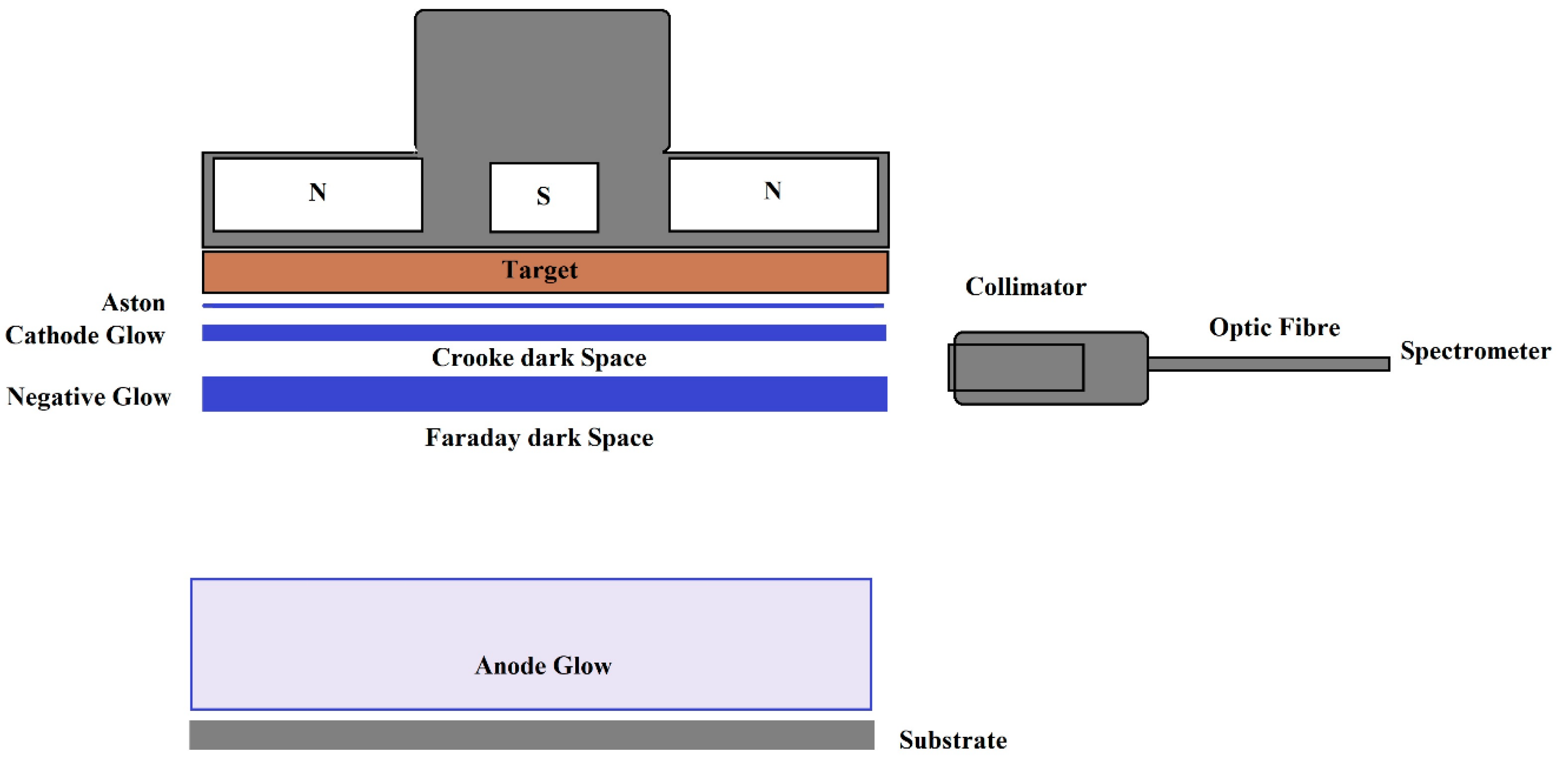
The glow discharge of the plasma is, to a significant degree, representative of the plasma ingredients and their characteristics. The glow is simply associated with the quantity and energy status of all the excited atoms and ions present in the plasma. As such, this glow can hold a significant amount of information that may be utilized to predict the properties of the films produced via the sputtering plasma. The plasma glow can be divided into five distinct layers, as illustrated in Figure 1 [4]. Directly adjacent to the target is a narrow layer known as the Aston dark space, which has a very low energy value [5,6,7]. The energy increases dramatically in the next layer [7], named the cathode glow due to its high luminosity [4]. After the cathode glow, there is the Crooke dark space; here all applied voltage is dropped, and it is from this region that the positive ions are accelerated towards the target. The Crooke dark space must be maintained, otherwise sputtering does not occur. Increasing the current density or chamber pressure decreases the space [8]. The negative glow region follows the Crooke dark space. Secondary electrons ionize gas atoms here, maintaining the sputtering process [4]. Finally, the Faraday dark space marks the full extent to which the ion sheath extends into the plasma [5]. The ion sheath, cathode sheath, or cathode fall, is the distance within which the voltage at the target exerts an attractive force into the plasma chamber [9,10]. Beyond the sheath, the chamber extends to the anode in what is known as the positive column. At the substrate, a small glow region and dark space occur (known as anode glow and anode dark space, respectively) [6,7,8,9,10].

The extent of the ion sheath into the plasma chamber is dependent on the electron density, temperature, and chamber pressure. Moving the substrate closer to the sheath, however, does not decrease the sheath size, only the width of the positive column. If the substrate anode is placed inside the sheath, the glow discharge is extinguished [6].

An important development in plasma sputtering was the addition of magnets behind the target, in what is known as magnetron sputtering. This causes a magnetic field to develop, which confines the plasma near the target surface and promotes increased gas ionization and target bombardment, as well as decreasing the substrate heating [11]. These magnets are arranged in such a way that the magnetic field is present between the edge and the center of the target, confining the plasma near the target, as shown in Figure 1 [11].

Magnetron sputtering can be described as either conventional or unbalanced. Conventional magnetron sputtering occurs when the central and side magnets are of equal power. However, problems arise in this system because the dense plasma causes scattering of the target atoms as they make their way to the substrate, decreasing the deposition rates [3,4,5,6]. Unbalanced magnetron sputtering, on the other hand, has stronger outer magnets, which make the plasma spread more evenly through the chamber. This increases the deposition rates but causes more defects in the substrate’s thin film. For high-accuracy applications, conventional magnetron sputtering is more desirable, despite being less efficient and slower. In our experiments, we work with conventionally balanced magnetrons.

The power supplied to the magnetron can be radio frequency (RF)-pulse-based or direct current (DC)-based. A serious problem with DC sputtering is that, when depositing a dielectric or non-conducting material, such as a TCO, positive ions accumulate at the surface of the target [9]. The positive ions neutralize the target voltage, leading, eventually, to the complete cessation of the sputtering process. Positive-ion build-up can also cause regions of high current and low voltage, as opposed to the normal low current and high voltage that runs the sputtering process [9]. This results in arcing, rapid heating, and a micro-explosion of the liquefied target, leaving droplets on the substrate that degrade the quality of the thin film [9]. To solve this problem, a RF pulse-based voltage can be applied to the target. While the voltage is positive, electrons from the plasma are attracted to the target, neutralizing the positive ions at the target surface. This is known as RF plasma sputtering. It is better for the homogeneity of the thin film and for its adhesion to the substrate [12].

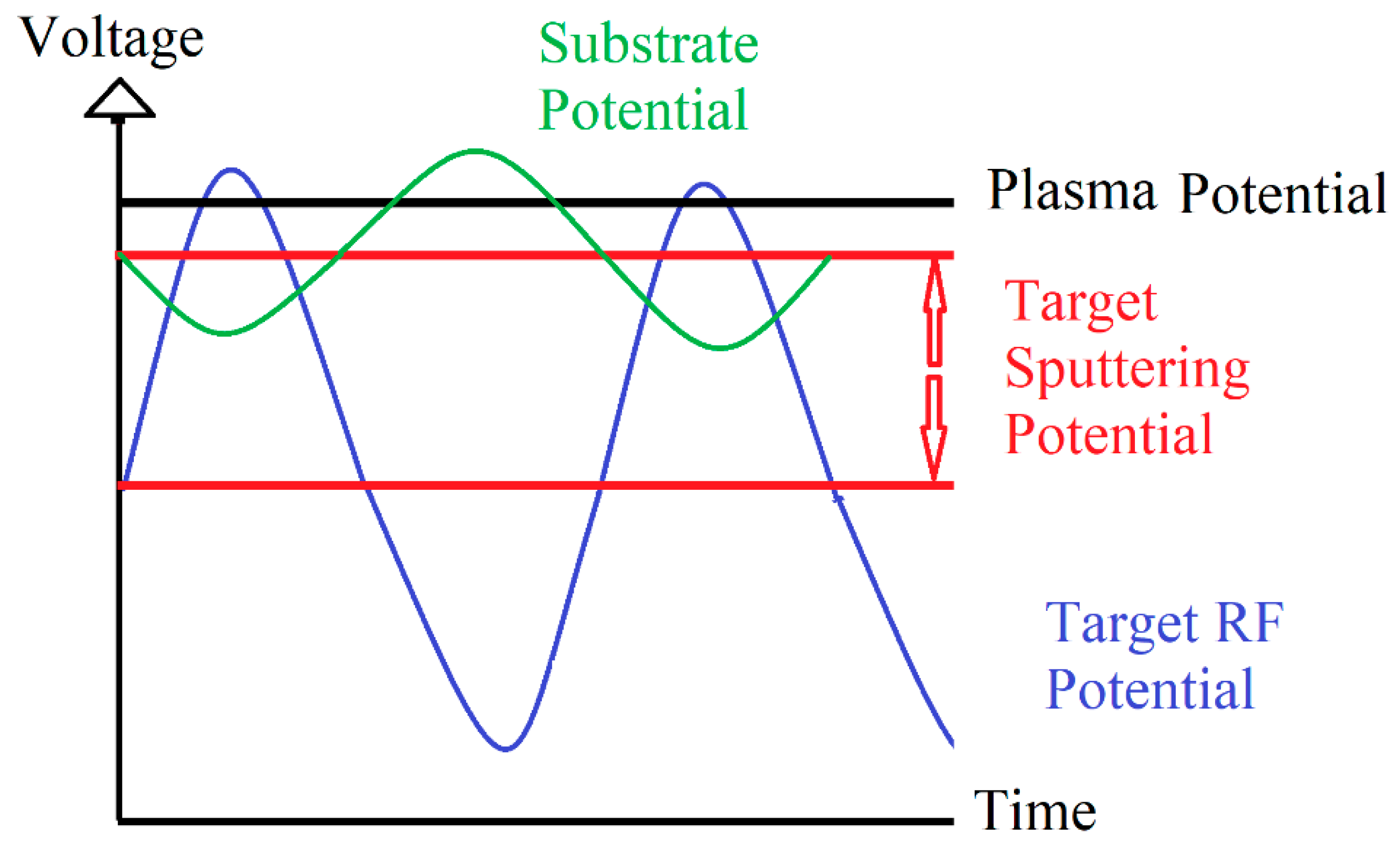
The AC voltage source in RF sputtering must be of the correct frequency. If the frequency is too low, positive ions neutralize the target during the negative half-cycle and electrons neutralize it during the positive half. In this situation, no ion sheath can develop; thus, no sputtering can occur. Because electrons have a smaller effective mass than ions, they respond to the change in target polarity more rapidly than ions. Therefore, if the AC frequency is increased, the electrons neutralize the target, whereas the slower ions do not have enough time. As a result, negative charge builds up on the target, and the ion sheath develops, allowing sputtering to occur. Studies show that the lowest possible frequency needed for sputtering is 10 kHz. Currently, the standard frequency for RF sputter systems is 13.56 MHz [9]. Figure 2 shows the voltages in RF sputtering, with the target potential shown in green.

Many variables influence the outcomes of the sputtering process: the RF power, the gas pressure, the deposition time, the angle of the target with respect to the substrate, the distance between the target and the substrate, the type of substrate, the thickness of the film, and the substrate temperature all have an effect on the thin film’s properties [12]. The three most important parameters, however, are the homologous chamber temperature, the sputter yield, and the energy of the bombarding ions. These characteristics are governed predominately by the plasma power [11].

The rate of deposition, or sputter yield, is measured by the ratio of atoms ejected from the target to high-energy ions incident on the target, as Equation (1) shows [13,14].

$${\rm Y}=\frac{\left(number of ejected particles\right)}{\left(number of incident particles\right)}$$

(1)

The sputter efficiency is usually measured in ${\rm Y}$ per watt of power applied [13].

The binding energy of the target material is the energy level that must be reached or surpassed for an atom to be ejected from its surface. This energy varies, depending on the effective mass of the target atoms and bombarding ions. Lower binding energies lead to more efficient sputtering [13]. Ions must have a sufficiently high energy on collision with the target for sputtering to occur, which is about 25 eV. Below this energy level, no sputtering can occur, regardless of incident ion numbers. At very high energies, however, sputtering rates also decrease. This is due to the ions penetrating too deep into the target. The energies of the electrons incident on the target have no effect on the sputtering process because the energy is too small to induce the collision cascade [3].

An atom is ejected from the target in a process known as the momentum collision cascade. The energetic ion incident on the target surface sets off a series of interatomic collisions in the target surface, ultimately resulting in an atom being ejected from the target [9,10,11,12,13].

Since sputtering is fundamentally a transfer of momentum process, the sputter yield depends on the efficiency of the transfer of momentum between the energetic ions and the target. The highest rates of sputtering occur when the target material and bombarding ions have similar atomic masses [13]. Accordingly, the greater the mismatch between target and ion masses, the less efficient the sputtering. Using the noble gas that has the closest atomic mass to the sputter target ensures maximum efficiency in this regard [13].

Depending on the energy of the incident particles, Powell et al. [13] identified four different physical outcomes of the collision cascade. Between 0 and 50 eV, sputtering only occurs in very-high-density plasmas and the yield is very poor [14,15,16]. Practical and commercial PVD sputtering lies in the moderate energy range of 50–1000 eV [17]. An ion impacting a target with energies between 1000 and 50.000 eV causes a dense target-atom cascade, in which all the atom-to-atom bonds are broken. At energies greater than 50,000 eV, the ions are implanted deep into the target, and few atoms are sputtered [13].

The angle of incidence of the bombarding ions affects the sputter yield [13,14,15,16,17,18]. Particles impacting the target at 90° emit fewer sputtered atoms than ions incident at shallower angles [18]. This is because collision cascades at shallower angles occur near the target surface, resulting in a greater likelihood of an atom being sputtered out. If the angle is too shallow, however, the ion simply bounces off the surface of the target without causing any sputtering. The ideal sputtering angle is between 45° and 50° [13,19,20,21]. In RF sputtering, however, inclining the target does not improve the angle of incidence of the ions because the plasma sheath is parallel to the target and the ion impact on the target surface is always normal.

Powell et al. identify two types of transport that occur at different chamber pressures: ballistic transport and diffusive transport. Ballistic transport occurs at low pressures (1.33 to 1.33 × 10⁻⁵ mbar). The sputtered atoms travel directly to the substrate, with few or no collisions to slow them down. Consequently, they arrive at the substrate with high energies [13,14,15,16,17]. The atoms are implanted into the growing sample, resulting in a finely grained thin film with good adhesion to the substrate. Diffusive transport occurs at pressures of tens of millibar or above. Collisions between the sputtered atoms cause them to lose energy. The electrostatic forces between the atoms also increase as they slow down. The grain sizes of the thin film are large, and the deposition is less likely to be homogenous.

Other factors, such as target positioning, can alter the properties of the plasma and thin films produced [22]. This occurs when other gasses, apart from the main working gas, are present in the chamber, or when any object within the chamber emits atoms in the form of gas. The presence of such gases in the system should alter the property of the plasma emission.

Overall, the emissions of the plasma glow reflect the information associated with the micro-environment of the plasma. Considering that a digital twin is a virtual representation serving as the digital counterpart of a physical process, the information embedded in the glow of the sputtering plasma can be utilized as a source of digitally interpretable data, which can form an interface between the actual physical sputtering process and its digital twin for forecasting and predicting the performance of the process.

2. Experimental Methods

2.1. The Concept

The glow from the plasma is a representation of the plasma ingredients, its constituents, and their states. It can be assumed that a vast amount of information is embedded in the plasma glow. Our objective here is to extract and exploit this information and correlate it with the parameters that are implemented during plasma formation. As these parameters ultimately govern the quality and properties of the thin films produced via this method, this is a step toward defining a digital twin for the sputter-deposition system.

In these experiments, we fitted seven different targets:

• Pure zinc oxide,
• Pure indium oxide
• IZO (indium oxide, zinc oxide) 70:30 ratio
• IZO (indium oxide, zinc oxide) 60:40 ratio
• IZO (indium oxide, zinc oxide) 50:50 ratio
• IZO (indium oxide, zinc oxide) 40:60 ratio
• ITO (indium oxide, tin oxide) 90:10 ratio

With each of these targets fitted into the magnetron, we generated a plasma under various operating conditions, whereby power, gas-flow rate, and working gas purity (using either pure argon or argon with 5% hydrogen content) were altered. With each experiment, we collected the spectral data associated with plasma glow.

Our primary objective was to investigate how accurately a deep-learning model (convolutional neural network models) trained with the spectral data would predict the following parameters using only the spectra of a sputtering plasma:

• Generation power;
• Gas-flow rate;
• Level of indium and zinc content in the target;
• Presence of hydrogen in the chamber;

2.2. The Experiment

The RF sputtering system used in this experiment was the V6000 confocal sputter-deposition system, built by Scientific Vacuum Systems limited (SVS Ltd., Wokingham, UK). The vacuum chamber is 400 mm × 400 mm × 400 mm and contains three 6-inch magnetrons. The collimator optic probe (Plasus GmbH, Mering, Germany), installed to measure the spectral output of the plasma, was placed in the front pointing back across the magnetron in use so that it was perpendicular to the plasma glow (Figure 1 and Figure 3). It collected light 15 mm from the target surface and 40 mm from the edge of the target. The light captured by the collimator was guided to a high-precision spectrophotometer (Plasus GmbH, Mering, Germany) via a quartz fiber-optic cable.

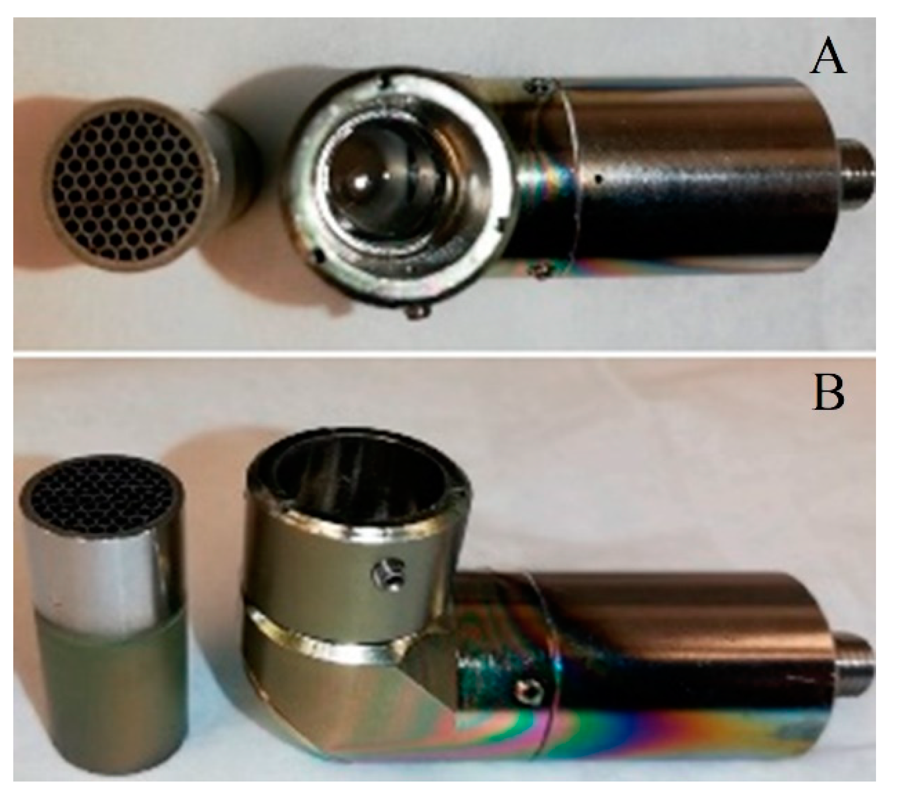
To prevent sputtered material covering the collimator lens, a honeycomb-like structure was fitted to the front, as illustrated in Figure 4.

The spectral data from the plasma were collected by fitting seven different targets in the magnetron and collecting spectral data under varying plasma powers and gas-flow rates, as depicted in Figure 5.

2.3. The Data

These experiments generate a large quantity of numerical data. The spectral emissions were collected from 204 nm to 1104 nm at 0.2 nm intervals, which means each single reading was an array of 4500 numbers representing emission peaks at particular wavelengths. For each sample, 2 random spectra were selected for training the neural network model. Therefore, the overall data set was a matrix of 588 rows and 4500 columns.

As we intended to use computer-vision-based deep learning to create our model, we needed to convert the 1-dimensional array associated with the spectral data into a 2dimensional tensor.

We took two approaches to convert the 1-dimensional array into 2D:

• Basic cut and stacking. As illustrated in Figure 6, the 4500 long array associated with the spectra was cut into 50 segments and stacked to form a matrix of 50 × 90 pixels, as illustrated in Figure 6.
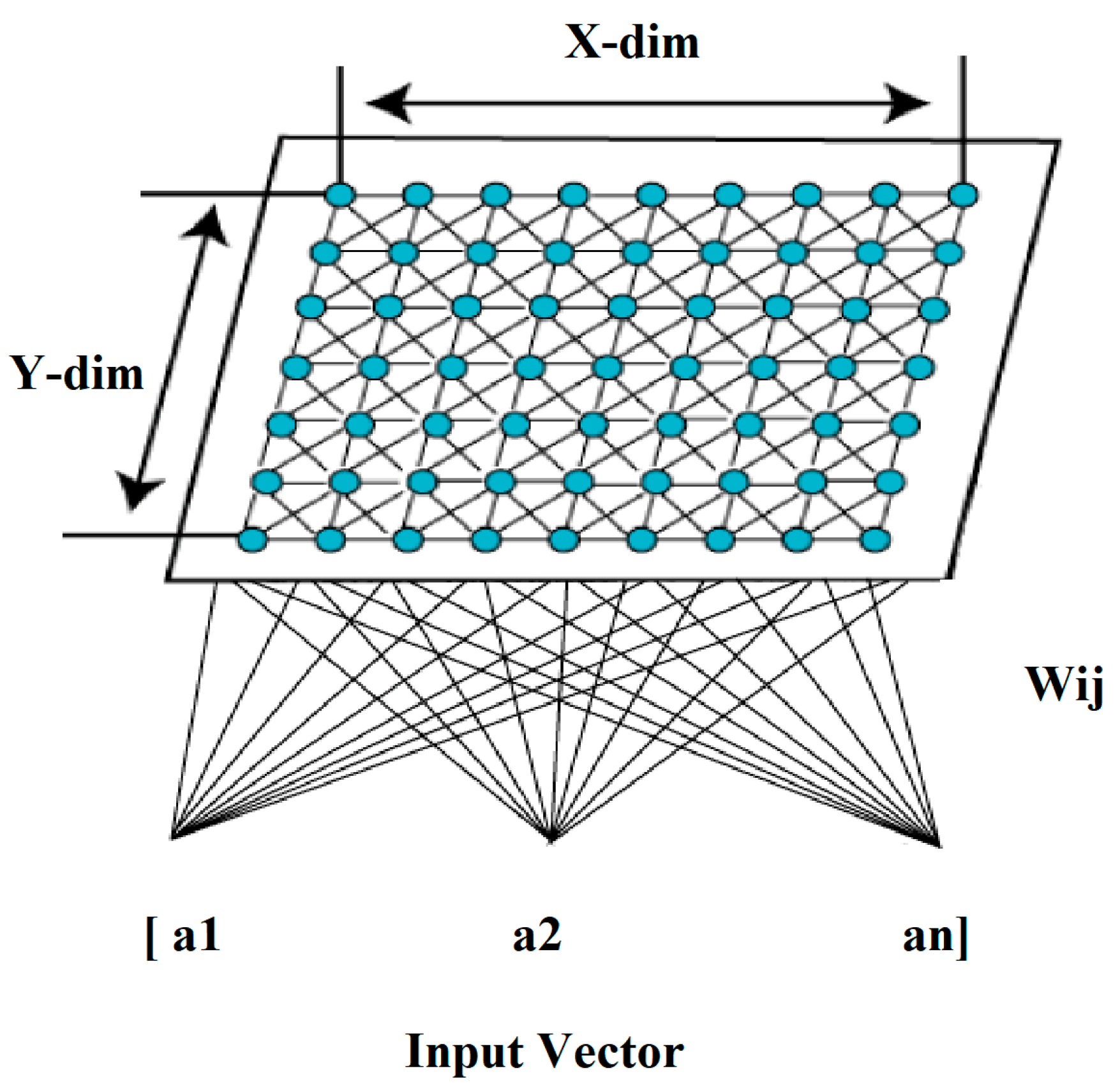
• By implementing an unsupervised machine-learning technique called self-organizing map (SOM), forming a 2-dimensional array of 90 × 90 pixels. The SOM illustrated in Figure 7 is an algorithm that was introduced by Teuvo Kohonen, acting as a non-supervised clustering algorithm capable of presenting multidimensional feature data into a two-dimensional map of clusters [23].

It is important to highlight the fact that prior to forming the 2-dimensional matrices from the spectral data, they were scaled via min-max scaling method, which arranges the values on a scale between zero and one:

$$x\left(\min \max \mathrm{scaled}\right)=\frac{x- \min \left(x\right) }{\max \left(x\right)- \min \left(x\right)}$$

(2)

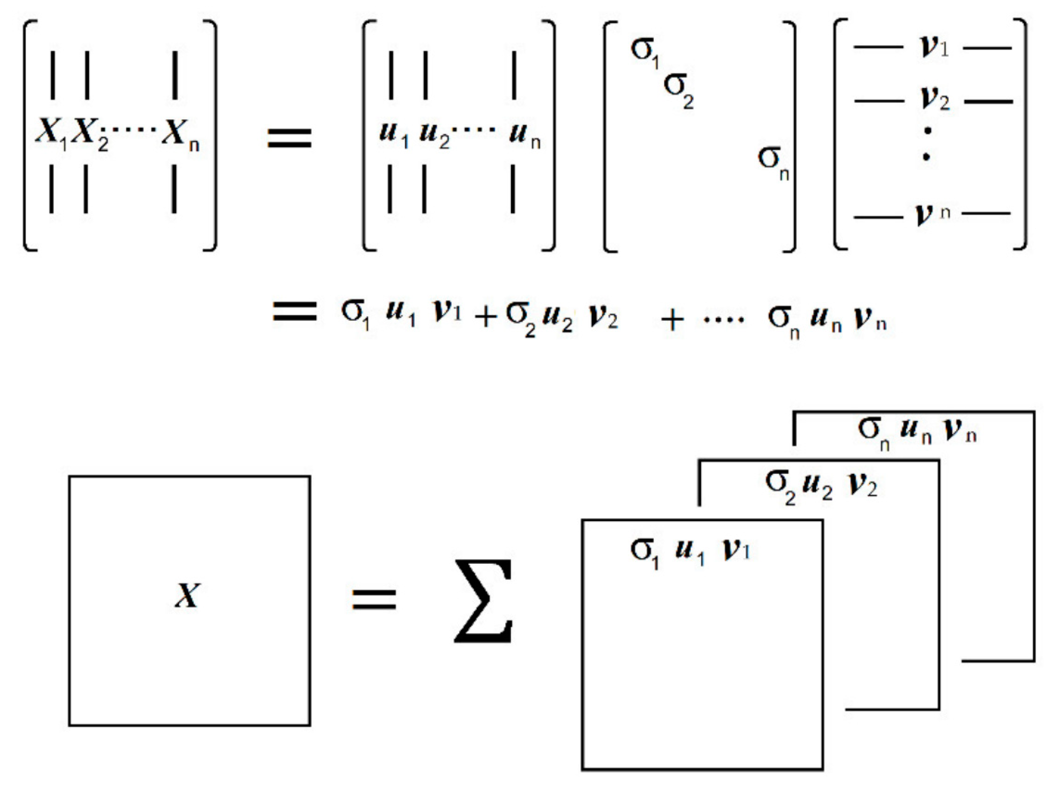
Once the 2-dimensional images were formed, we also carried out a singular value decomposition (SVD) on the 2-dimensional matrices and then reconstructed the matrix by first layer of the SVD model. The objective of this operation was to gain an insight into the level of information embedded into the 2-dimensional matrices that we constructed from the spectral data. As there may have been some noise hidden in the spectral data, the SVD decomposition and reconstruction of the first layer may have eliminated the hidden noise signals, thereby generating more accurate predictions. The basicSVD operation and reconstruction is illustrated in Figure 8.

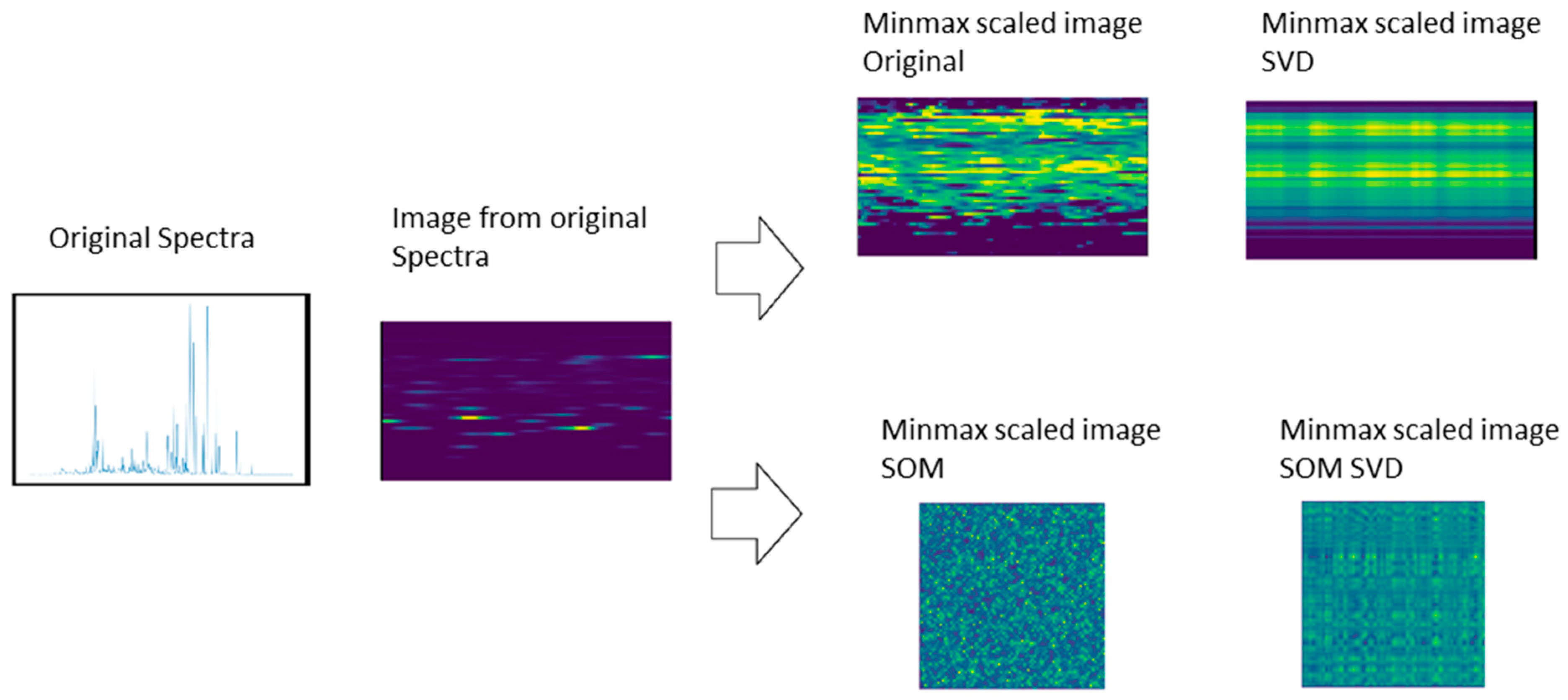
Therefore, every spectral datum that related to a particular target at particular RF plasma power and gas-flow rate and specific working gas was converted into four separate images. This family of images was then used to train a convolutional neural network (CNN) model. Figure 9 illustrates the formation of four separate images from every spectral datum. Given that we had 588 spectral data, we now had 588 X 4 images belonging to each of the four image groups, which were used separately to train a CNN.

To appreciate how difficult it was to distinguish the glow of the plasma under various conditions, some plots of the plasma spectrum are presented in Figure 10, Figure 11, Figure 12 and Figure 13. Figure 10 presents the emission spectrum associated with 9-, 7-, and 3-standard-cubic-centimeter-per-minute argon flow rates overlayed (A) and also in a segregated format (B). In Figure 11, the effect of the presence of 5% hydrogen in the argon gas in overlay and segregated form is presented. In Figure 12, the emission spectrum associated with the four different target materials is presented. These spectra reveal some differences if precise attention is paid. However, these examples are presented here to illustrate the complexity and precision of the spectra in detail.

Our objective was for the CNN model to be able to calculate certain parameters, such as the gas-flow rate, plasma power, and presence of hydrogen, through computer vision assessment of these spectra. This is further illustrated in Figure 13, where a section between 400 and 600 nm is magnified to illustrate the difference between spectra of the same target material at same plasma power and pressure, but with 5% hydrogen impurity in one.

2.4. The CNN Model

The four classes of image forms were used separately to train the CNN model. The structures of the CNN model for regression analysis and classification analysis were the same except for the final layer. The structure of the CNN model is presented in Figure 13. The image data were submitted to two steps of convolution and max pooling, consecutively, prior to being flattened into a single vector. The vector was then used to train an artificial neural network model with four dense layers containing 5000, 5000, 100, and 20 neurons each, all bearing a rectified linear-unit function.

For regression analysis, a final dense layer with a single neuron was used for predicting the gas-flow rates and plasma power. The loss function used for the model training was mean squared error.

For classification analysis, the final dense layer with a single neuron was set up with a sigmoid activation function. The loss function used for model training was binary cross entropy.

Both the regression and the classification models utilized an Adam optimizer with a learning rate of 0.001.

Figure 13. The structure of the CNN model. The model is composed of two consecutive convolutional and max_pooling layers for feature extraction; the output shapes are presented. A flattened layer was used to convert the resulting feature maps in one-dimensional array via the flattening. All were activated by a rectified linear-unit function. The ANN section of the model has four deep layers, containing 5000, 5000, 100, and 20 neurons activated by a rectified linear-unit function, leading to a single output neuron.

Figure 13. The structure of the CNN model. The model is composed of two consecutive convolutional and max_pooling layers for feature extraction; the output shapes are presented. A flattened layer was used to convert the resulting feature maps in one-dimensional array via the flattening. All were activated by a rectified linear-unit function. The ANN section of the model has four deep layers, containing 5000, 5000, 100, and 20 neurons activated by a rectified linear-unit function, leading to a single output neuron.

A vital part of this study was its focus on the treatment of the numerical data prior to model training. It is a well-known fact that for all deep-learning models, the data need to be scaled or standardized.

However, we also carried out a secondary step in scaling the data. For each emission spectrum, the peak intensities were summed, and every intensity to the resolution of 0.2 nanometers was divided by the total sum. The importance of this step is vital to the performance of the models. We specifically performed this operation because the temperature of ions and electrons in the plasma are directly proportional to their random average kinetic energy, while Maxwell distribution governs the distribution of velocities for each particle when thermal equilibrium conditions apply. The same temperature was assumed for electrons, ions, and atoms in the plasma, and the plasma temperature was considered the temperature of the electrons [22,24]. From the plasma spectral emissions, two spectral lines can be chosen from the same species (for example, argon) and ionization stage, where there is a large difference in the upper energy level. Ultimately, by taking a ratio (I₁)/(I₂) of the intensities of the selected lines, the temperature of the electron can be calculated in electron volts [24].

This method is the simplest approach to calculating the temperature of the plasma, and its accuracy is conditional on using two lines, with a maximum difference in their upper energy states.

Therefore, there are hidden patterns associated with each individual plasma when ratio of peak intensities is considered. Therefore, by implementing the operation of representing each 0.2-nanometer peak intensity as a fraction of the total intensities, we provide the neural network model with hidden features related to the microenvironment of the plasma for the model training.

3. Results and Discussion

Overall, we used 2352 images (588 images per method of 2-dimensional matrix formation) associated with various targets—working gas pressures, plasma power, and hydrogen impurity—that were present in the argon gas. We randomly selected 80% of our data for training the models and used the remaining 20% to evaluate the prediction of the models and their accuracy.

A very interesting initial observation was that the models were trained best on the data sets for which the peak-intensity ratio operations were carried out. In fact, without this step, standard scaling alone was insufficient to train the models, as extremely poor results and prediction were observed. However, the min-max scaling resulted in desirable accuracies, as in a sense it converts the data points to a minimum–maximum range of 0 to 1. However, once the peak-intensity ratio operation was carried out, standard scaling and min-max scaling were equally good for training the models for desirable accuracy. However, all the results presented in this report are associated with data that were min-max scaled. We investigate the results for each set of samples and experiments separately.

When presenting our results, ‘Original’ refers to the min-max-scaled stack-overlay-formed images. ‘Original_SVD’ refers to the first-layer reconstruction of the original image after SVD decomposition.

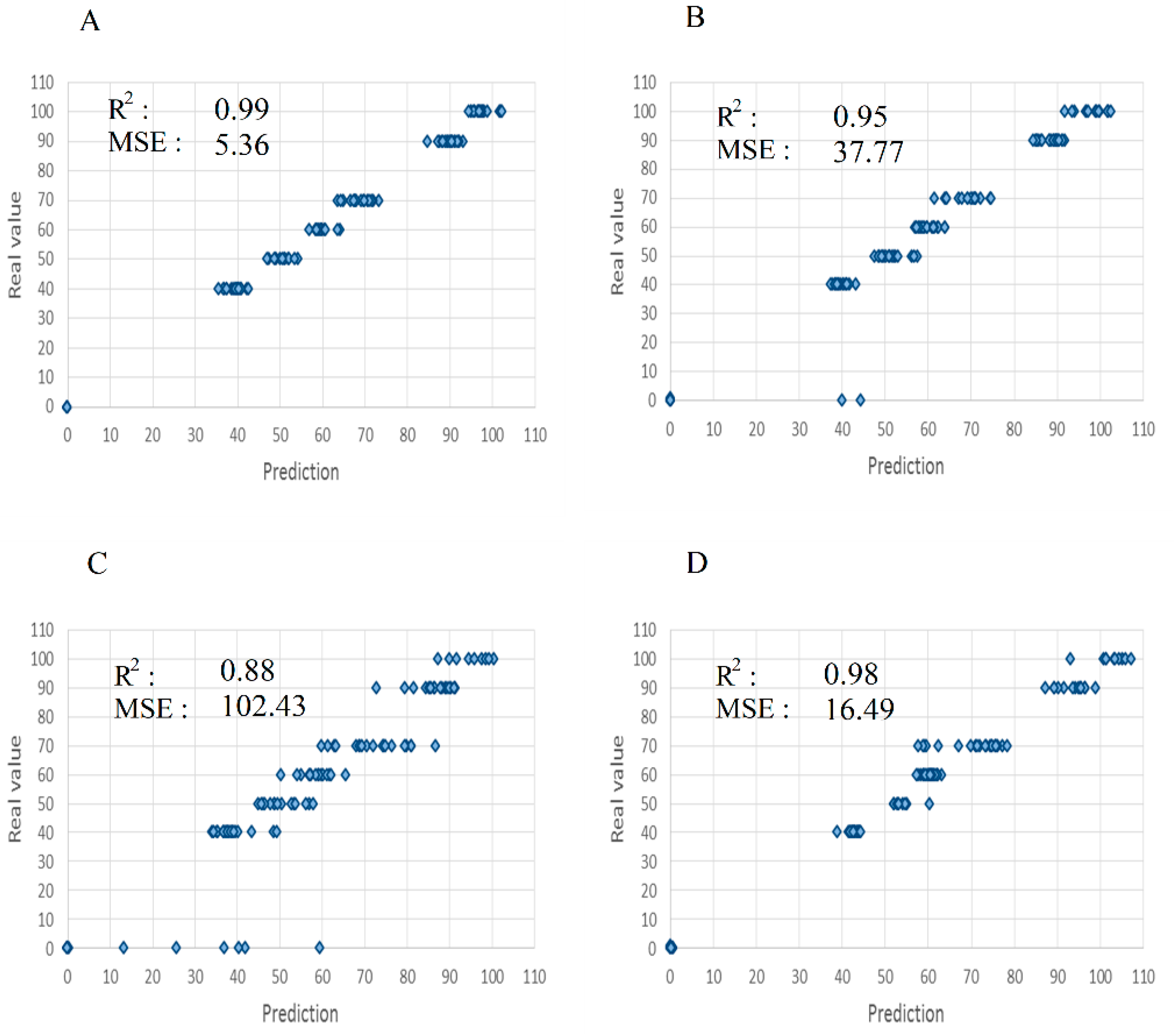
‘SOM’ refers to images generated from the spectra via the self-organizing map method and ‘SOM_SVD’ refers to the first-layer reconstruction of the SOM image after SVD decomposition. The results of predicting the zinc concentration in the target are presented in Figure 14. It can be seen that SVD reconstructions of the SOM-formed images performed less effectively.

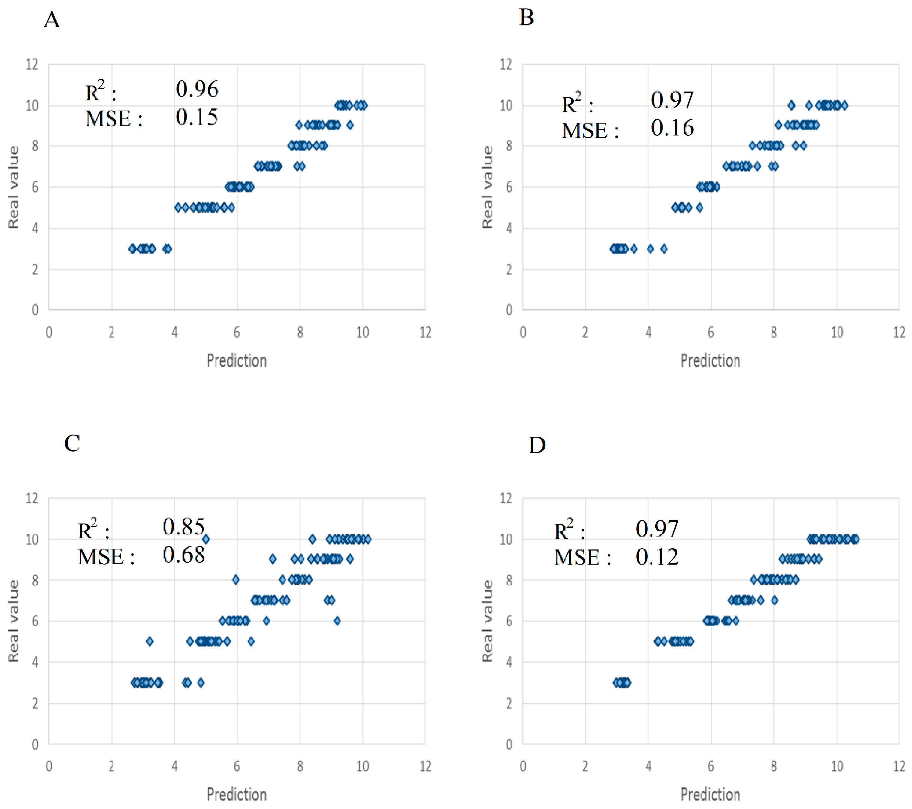
The results of predicting the indium concentration in the target are presented in Figure 15. Once again, we can see that the SVD reconstruction of the SOM-formed images performed less effectively. Figure 16 and Figure 17, respectively, demonstrate the predictions of the gas-flow rate and plasma power.

Out of all the results, we can see that the SVD reconstruction of the SOM model (SVDS) produced the least accurate predictions. The original stack-overlay method of reconstructing a two-dimensional array from the one-dimensional array of the spectra seems to be sufficient for training the CNN model for accurate predictions.

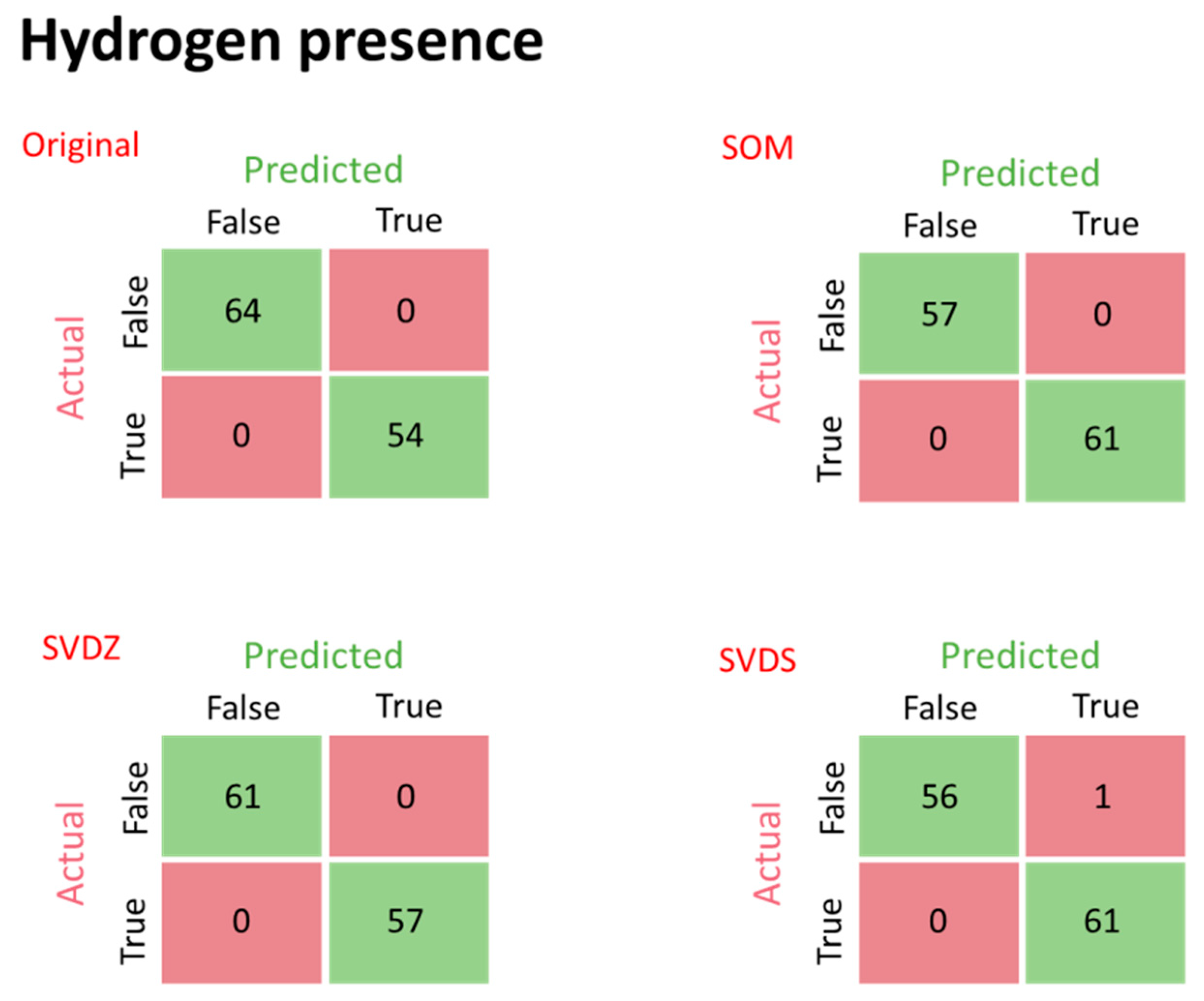
When the model was used as a classifier rather than a regressor to predict the presence of hydrogen impurity and impurity in the indium-oxide-based target, we obtained excellent results with all forms of two-dimensional conversion techniques, as presented in Figure 18 and Figure 19. The accuracy metrics associated with the hydrogen presence and indium-oxide target purity are presented in

Table 1. Confusion matrix of model classification associated with Hydrogen presence and impurity in the indium oxide target.

Hydrogen Presence
Model	Accuracy	Recal	Precision
SOM_SVD	0.99	1	0.98
ORIG_SVD	1	1	1
SOM	1	1	1
ORIG	1	1	1
Impurity presence in InO Target
Model	Accuracy	Recal	Precision
SOM_SVD	0.99	1	0.94
ORIG_SVD	1	1	1
SOM	0.99	0.95	1
ORIG	1	1	1

, Presenting the accuracy metrics of the CNN model’s performance trained with images formed from the four methods of two-dimensional image formation; presence of hydrogen in the working gas and impurity in the indium-oxide target.

4. Conclusions

The results presented in this report (Figure 14, Figure 15, Figure 16, Figure 17, Figure 18 and Figure 19) clearly demonstrate the potential of deep learning and, in particular, computer-vision-based CNN models as the tool of choice to be utilized in associating the spectra emissions of plasma to the operating conditions of sputtering units. Plasma power and gas-flow rates do indeed affect plasma glow and its spectral characteristics. Higher plasma power can lead to higher energy ions and higher rates of excitation, which also affect the property of the thin film deposited while demonstrating a unique glow feature in the plasma emission. Higher gas-flow rates increase the chamber pressure, resulting in a greater flux of atomic collisions and variation in the ion distribution. This, in turn, affects the property of the thin film deposited. Our models were shown to be successful at predicting various features associated with the process, such as (wt%) content of the target ingredients in Figure 14 and Figure 15 and the gas-flow rate and plasma power, as presented in Figure 16 and Figure 17. The model also demonstrated the ability to predict the presence of an additional gas (hydrogen) as a 5% impurity in the argon working gas and to assess the purity of the target itself, as presented in Figure 18 and Figure 19.

All these parameters are critical in defining the properties of the thin films produced via this form of plasma sputtering. When neural networks can associate the spectral features of the plasma with a numerical assessment of these critical operating features, they can also be implemented to predict the properties of thin films. In a previous study, we demonstrated this by focusing on a single sputtering target (indium zinc oxide) and assessing the electrical property of the produced thin films [25]. In this study, we extended the range of the target materials to further validate the observations in our previously reported study.

Therefore, we believe that further research into the implementation of deep -learning models in the process of plasma-assisted thin-film deposition processes can lead to the construction of a digital twin for sputter-deposition processes, which are responsible for preparing many of the thin films implemented in various common products.

Since the concept of the perceptron was proposed by Frank Rosenblatt in the 1960s [25], through the pioneering works of Hinto, LeCun, and Bengio in the 1980s [26], further developments have frequently risen in this emerging field of computer science and, currently, with companies such as Google and Facebook taking the lead in further exploiting its potentials, we are witnessing the emergence of increasingly complex deep-learning models with extended dimensions of numerical analysis. Hence, there is a need for scientists in other conventional fields, such as material science, to integrate and implement this technology in their research. In our experiments, we used a static CNN construction and trained it with the images we formed from the four described two-dimensional images. By further adjusting the CNN model, higher accuracies are achievable. It was shown that the spectral data can be easily used to form an image that can benefit from the power of modern computer-vision deep-learning models. This simple approach even outperformed the more complex SOM method of two-dimensional array formation. The only challenge to consider is the necessary data. Deep-learning models perform more accurately and efficiently when large amounts of data are available. Implementing deep-learning models in existing engineering or materials-engineering topics will require an approach involving the presence or collection of structured data. Therefore, efforts focusing on generating a vast library of spectral emissions associated with the sputtering of various materials will be a key step toward the formation of a digital twin for plasma-sputtering process. We previously demonstrated how these models can be used to predict the physical properties of thin films [25], with a focus on a single material. Here, we showed that these models are capable of predicting the nature of plasma at a high level of precision and, therefore, we can conclude that they can be instrumental in predicting various other material properties associated with thin films produced via sputtering.