Effects of Magnetohydrodynamics Flow on Multilayer Coatings of Newtonian and Non-Newtonian Fluids through Porous Inclined Rotating Channel

Abstract

In this study, we investigated multilayer coatings fully developed with steady Newtonian and non-Newtonian fluids through parallel inclined plates. The channel was rotating about the $y$-axis with angular velocity $\Omega$. The channel contained three regions; Region 1 and Region 3 were filled with Newtonian fluid, while Region 2 had Jeffrey fluid through a porous medium. The governing equations were formed by using Navier stokes and energy equations. The equations were coupled and were non-linear due to the involvement of Darcy’s dissipation terms. The systems of equations for Region 1 and Region 3 were solved analytically, while the equations of Region 2 were solved by using the regular perturbation method. The effects of governing parameters such as magnetic field, Grashof number, the ratio of heights, angle of inclination, and ratio of viscosities on velocity and temperature were investigated, and the results are presented graphically in this paper. It is noted that the increase in buoyancy force incorporated through the Grashof number and the angle of inclination enhanced the axial and transverse velocities and the temperature for the three layers. We found that the Nusselt number increases by increasing the couple stress parameter and magnetic field parameters, and skin friction decreases at the lower plate. The main observation is that temperature and both velocity profiles increased in Region 2 with the increase in the Jeffrey parameter.

1. Introduction

In recent decades, non-Newtonian fluid has become a valuable area of research because of its extensive applications in engineering and technology, such as in plastics production, production of lubricants, food clearing, and motion of biological liquid. Several models have been put forward to estimate and narrate the physico-chemical conduct of non-Newtonian fluid. The major non-Newtonian fluid category is Jeffrey fluid, which plays an important role in the present work. This fluid is an approximately plain viscoelastic that shows relaxation and retardation effects together. Akram and Nadeem [1] presented an exact and close-form of Adomian solutions of the peristaltic motion of a two-dimensional Jeffrey fluid in an asymmetric channel under the effects of induced magnetic field and heat transfer. They observed that the pressure rise for the sinusoidal wave was less than the trapezoidal wave and greater than the triangular wave. Santhosh and Radhakrishnamacharya [2] examined the incompressible laminar magnetohydrodynamic Jeffrey fluid movement through a permeable channel in a thin tube and obtained an analytical solution for the equations of motion and continuity equation. They found that the effective viscosity increases with the Jeffrey parameter in the system. Abd-Alla et al. [3] analyzed the impact of gravity and the magnetic field of Jeffrey fluid in the channel. Dhananjaya et al. [4] studied the incompressible laminar fully developed natural convection flow and heat transfer of a Jeffrey fluid between two vertical parallel pates partially filled with porous medium and obtained an analytical solution for the governing coupled equations. Abd-Alla and Abo-Dahab [5] analyzed the influence of magnetic field and rotation effects on the peristaltic transport of a Jeffrey fluid in an asymmetric channel. Krishna Murthy [6] analyzed a two-dimensional MHD steady incompressible free convective Couette flow of Jeffrey fluid in a porous medium in the presence of heat sources and chemical reactions; the flow was generated due to constant normal suction/injection at the plates and a numerical solution was obtained by the shooting method. Raju et al. [7] reconstructed flow field equations solved numerically by Newton’s method onward with the Runge–Kutta method. Several investigations on recent trends in coatings and thin film modeling and application can be found in [8] and several studies referenced therein.

The presence of MHD two-phase motion between two parallel plates is of critical importance in engineering and technology. In chemical production, two-phase motion occurs in heat interchange equipment, gas–liquid coatings, fabrication, and chemical atomic reactors such as load columns, spray and sparkle columns, agitated vessels, etc. Another important area where understanding two-phase motion is vital is in nuclear reactor design (water-cooled atomic reactors and sodium-cooled quick breeder reactors, etc.). The steady magnetic field is applied to manage the framework of the material, refine non-metallic compounds and molten metals, cool unbroken filaments and strips, etc. The application of MHD occurrence has significant value in many technological fields such as medical science [9], direct numerical simulation of helical generator action [10], drag reduction within physical phenomena [11], and seawater propulsion [12]. Romig [13] investigated the effects of electric and magnetic fields on heat transmission to electrically conducting fluid. Rudraiah et al. [14] analyzed non-linear magnetoconvection and its implementation in the solar move problem. Shail [15] discussed the different region flow of plates in which one side of the plate was a conductor and the other side of the plate was insulated. Lohrasbi and Sahai [16] investigated the MHD two-region flow with heat transmission features in a horizontal station in which one region was electrically conducting and the other region was electrically non-conducting. Malashetty and Leela [17] carried out the preceding work and theoretical study on MHD heat transmission in two-region flow for short-circuit situations. Malashetty and Leela [18] investigated the MHD heat transmission in two-region flow by considering fluid in all phases to be electrically conducting for the open-circuit situation. Chauhan and Rastogi [19,20] examined heat transmission impacts and Hall current on MHD flow in a medium partially filled with a permeable channel in a revolving system. Seth et al. [21] presented the Hartman flow in a revolving system in the presence of a slanted magnetic field with Hall impacts.

For engineering and industrial implementation, researchers have considered the rotating fluid’s application in engineering. Fiza et al. [22] determined the rotational flow of Jeffrey fluid and MHD between two equal and similar plates with the effect of room current. Greenspan and Goodman elaborated on the study of fluid in a rotating system [23,24]. MHD in a rotating scheme and extended porous medium have been studied by Attia and Kotb [25]. Borkakoti and Bharali [26] contributed to the determination of heat transfer between two horizontally arranged plates. Vajravelu and Kumar [27] came up with the task of providing numerical and analytical solutions in a non-linear system. Das et al. [28] explained the concept of nano-fluids in science and technology. Mohyud-Din et al. [29] emphasized mass and heat transfer investigation, keeping in mind the flow of nanofluids between two parallel plates. Murty et al. [30] examined the rotating system and the MHD effects and heat transfer of two-fluid flow in a leaning channel that contained porous and fluid layers. Chitturi et al. [31] examined the convective flow between two parallel plates containing porous layers of fluids in a rotating system. The phenomena of highly coupled nonlinear differential equations constructed in different fluid coating models are tackled by different techniques [32,33,34,35,36,37].

In this paper, we develop a theoretical model for analyzing the convective flow of multilayer coatings of Newtonian and non-Newtonian fluids. The rotating channel contains three regions; Region 1 and Region 3 are filled with Newtonian fluid, while Region 2 is filled with Jeffrey fluid via a porous medium. For all the physical parameters, temperature is linear in Region 1 and Region 3 but nonlinear in Region 2. The governing highly non-linear and coupled equations are solved analytically with the regular perturbation method. The effects of governing parameters such as magnetic field, Grashof number, ratio of heights, angle inclination, and ratio of viscosities on velocity and temperature are investigated and depicted graphically.

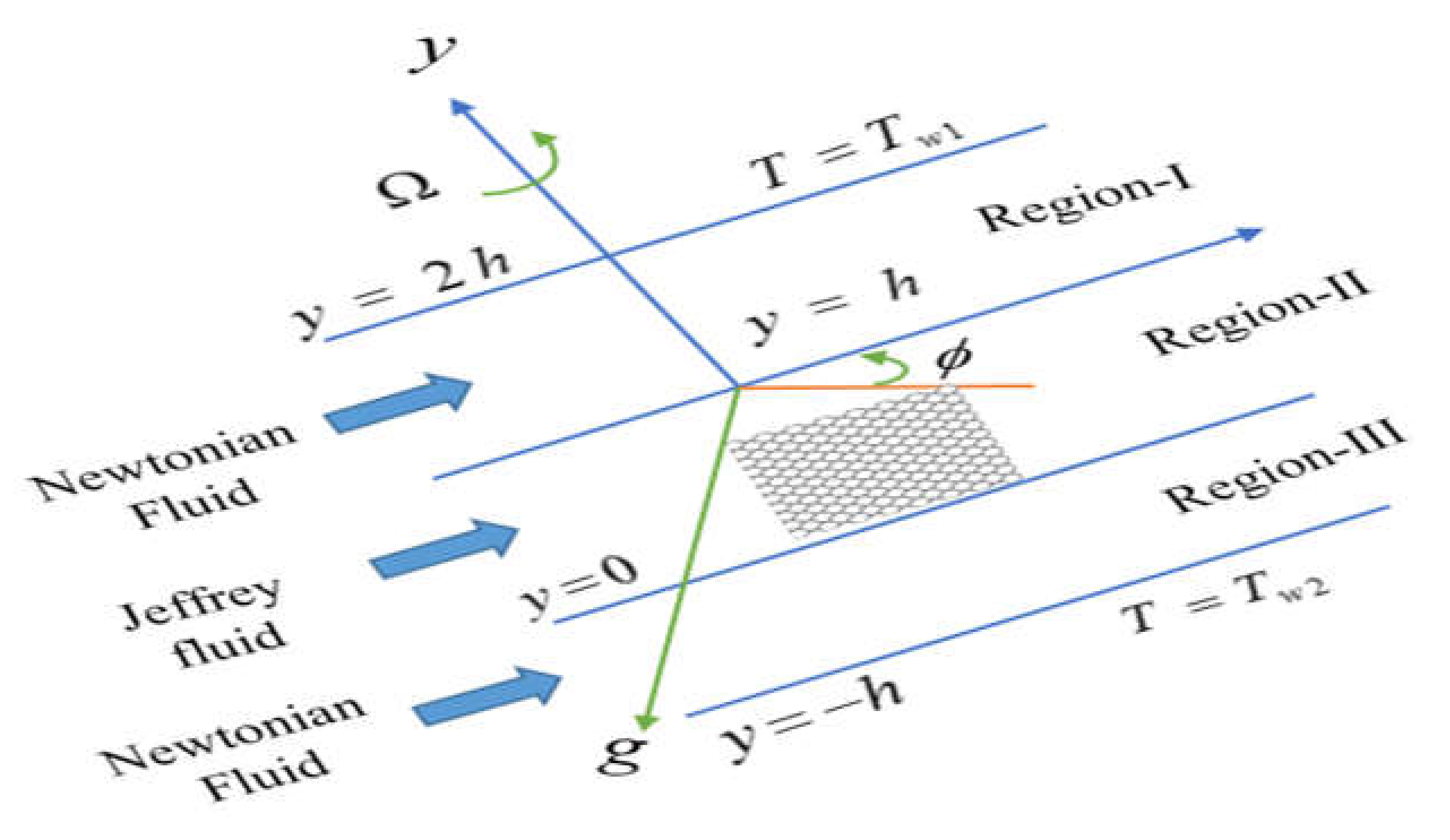
2. Formulation of the Problem

The steady flow of a multilayer fluid is between two infinite parallel plates along the $x$ and $z$ directions. The temperature of the upper plate $T_{w_1}$ and lower plate $T_{w_2}$ are kept constant, with $\varphi$ representing the angle of inclination of the channel with a horizontal surface. The geometrical representation of the problem is shown in Figure 1.

The regions with $-h\le y\le 0$ and $h\le y\le 2h$ contain Newtonian fluid. The porous region $0\le y\le h$ is filled with Jeffrey fluid of density ${\rho }_2$, electrical conductivity $\sigma ,$ dynamic viscosity ${\mu }_2$, thermal conductivity $k_2$, and porous materials of permeability $K$. The system is rotated with angular velocity $\Omega$ about the $y$-axis. The channel temperature gradient is $\Delta T=T_{w_1}-T_{w_2}$, whereas the pressure gradient $\left(-\partial p/\partial x\right)$ is constant. The fluid is assumed to be electrically conducting under the impact of a uniform transverse magnetic field of strength $B_0$ and is applied to the plates. The essential equation for Jeffrey fluid is $S=\frac{{\mu }_2}{I+{\lambda }_1}\left(I+{\lambda }_2\frac{d}{dt}\right)A$, where $S$ is the extra stress tensor, ${\lambda }_1$ is the ratio of relaxation to retardation times, ${\lambda }_2$ is the retardation time, and $A$ is the Rivlin–Ericksen tensor defined by $A=\left(\nabla V\right)+{\left(\nabla V\right)}^T$. The mathematical equations of motion and energy are given as [31,38]:

Region 1:

$${\mu }_1\frac{d^2{u}_1}{d{y}^2}+{\rho }_{1}g{\beta }_1\mathrm{Sin}\varphi \left(T_1-T_{w2}\right)=\frac{\partial p}{\partial x}+2{\rho }_1\Omega w_1+\sigma B_0^2{u}_1,$$

(1)

$${\mu }_1\frac{d^2{w}_1}{d{y}^2}=-2{\rho }_1\Omega u_1+\sigma B_0^2{w}_1,$$

(2)

$$\frac{d^2{T}_1}{d{y}^2}=0.$$

(3)

Region 2:

$$\frac{\partial s_{xx}}{\partial x}+\frac{\partial s_{xy}}{\partial y}+\frac{\partial s_{xz}}{\partial z}+{\rho }_{2}g{\beta }_2\mathrm{Sin}\varphi \left(T_2-T_{w2}\right)-\frac{{\mu }_2}{K}{u}_2=\frac{\partial p}{\partial x}+2{\rho }_2\Omega w_2+\sigma B_0^2{u}_2,$$

(4)

$$\frac{\partial s_{zx}}{\partial x}+\frac{\partial s_{zy}}{\partial y}+\frac{\partial s_{zz}}{\partial z}-\frac{{\mu }_2}{K}{w}_2=-2{\rho }_2\Omega u_2+\sigma B_0^2{w}_2,$$

(5)

$$\frac{d^2{T}_2}{d{y}^2}+\frac{{\mu }_2}{k_{2}K}\left(u_2^2+w_2^2\right)=0.$$

(6)

Region 3:

$${\mu }_1\frac{d^2{u}_3}{d{y}^2}+{\rho }_{1}g{\beta }_1\mathrm{Sin}\varphi \left(T_3-T_{w2}\right)=\frac{\partial p}{\partial x}+2{\rho }_1\Omega w_3+\sigma B_0^2{u}_3,$$

(7)

$${\mu }_1\frac{d^2{w}_3}{d{y}^2}=-2{\rho }_1\Omega u_3+\sigma B_0^2{w}_3,$$

(8)

$$\frac{d^2{T}_3}{d{y}^2}=0.$$

(9)

where $u_i$ and $w_i$ are $x$ and $z$ components of velocity, respectively, and $T_i$ is the temperature, with subscripts $i=1,2,3$ representing the value for the regions. The velocity becomes equal to zero at the wall due to the no-slip condition.

The respective boundary and interface condition with the above conditions for velocity and temperature distribution are:

$$\begin{array}{l}{u}_1\left(y\right)=0,w_1\left(y\right)=0,T_1\left(y\right)=T_{w_1}\hspace{1em}\hspace{1em}\hspace{1em}\hspace{1em}\hspace{1em}\hspace{1em}\hspace{1em}\hspace{1em}\hspace{1em}\hspace{1em} \mathrm{at} y=2h\\ \begin{array}{l}{u}_1\left(y\right)=u_2\left(y\right),w_1\left(y\right)=w_2\left(y\right),{\mu }_1\frac{d{u}_1\left(y\right)}{dy}=\frac{{\mu }_2}{\left(1+{\lambda }_1\right)}\frac{d{u}_2\left(y\right)}{dy} \mathrm{and} \\ {\mu }_1\frac{d{w}_1\left(y\right)}{dy}=\frac{{\mu }_2}{\left(1+{\lambda }_1\right)}\frac{d{w}_2\left(y\right)}{dy}, T_1\left(y\right)=T_2\left(y\right),k_1\frac{d{T}_1\left(y\right)}{dy}=k_2\frac{d{T}_2\left(y\right)}{dy}\end{array}\} \mathrm{at} y=h\\ \begin{array}{l}{u}_2\left(y\right)=u_3\left(y\right),w_2\left(y\right)=w_3\left(y\right),\frac{{\mu }_2}{\left(1+{\lambda }_1\right)}\frac{d{u}_2\left(y\right)}{dy}={\mu }_1\frac{d{u}_3\left(y\right)}{dy} \mathrm{and} \\ \frac{{\mu }_2}{\left(1+{\lambda }_1\right)}\frac{d{w}_2\left(y\right)}{dy}={\mu }_1\frac{d{w}_3\left(y\right)}{dy}, T_2\left(y\right)=T_3\left(y\right),k_2\frac{d{T}_2\left(y\right)}{dy}=k_1\frac{d{T}_3\left(y\right)}{dy}\end{array}\} \mathrm{at} y=0\\ u_3\left(y\right)=0,w_3\left(y\right)=0 , T_3\left(y\right)=T_{w_2}\hspace{1em}\hspace{1em}\hspace{1em}\hspace{1em}\hspace{1em}\hspace{1em}\hspace{1em}\hspace{1em}\hspace{1em}\hspace{1em} \mathrm{at} y=-h\end{array}\}$$

(10)

We can change Equations (1)–(10) into dimensionless forms by using the following [31] transformations:

$$\begin{array}{l}\frac{u_1}{{\overline{u}}_1}=u_1^{*},\frac{u_2}{{\overline{u}}_1}=u_2^{*},\frac{u_3}{{\overline{u}}_1}=u_3^{*},\frac{w_1}{{\overline{u}}_1}=w_1^{*},\frac{w_2}{{\overline{u}}_1}=w_2^{*},\frac{w_3}{{\overline{u}}_1}=w_3^{*},\frac{y_1}{h}=y_1^{*},\frac{y_2}{h}=y_2^{*},\frac{y_3}{h}=y_3^{*},\\ m=\frac{{\mu }_1}{{\mu }_2},S_{xx}=0,S_{xy}=\frac{{\mu }_2}{\left(1+{\lambda }_1\right)}\frac{\partial u_2}{\partial y},S_{xz}=0,S_{yy}=0,S_{zz}=0,S_{yz}=\frac{{\mu }_2}{\left(1+{\lambda }_1\right)}\frac{\partial w_2}{\partial y},\\ M_1=\sqrt{\frac{\sigma }{{\mu }_1}}{B}_{0}h,{\theta }_1=\frac{\left(T_1-T_{w2}\right)}{\left(T_{w1}-T_{w2}\right)},{\theta }_2=\frac{\left(T_2-T_{w2}\right)}{\left(T_{w1}-T_{w2}\right)},{\theta }_3=\frac{\left(T_3-T_{w2}\right)}{\left(T_{w1}-T_{w2}\right)},R^2=\frac{\Omega h^2}{{\nu }_1},\\ Gr=\frac{g{\beta }_1{h}^3\left(T_{w1}-T_{w2}\right)}{{\nu }_1},b=\frac{{\beta }_1}{{\beta }_2},Pr=\frac{{\mu }_1{C}_p}{k_1},\lambda =\frac{h}{\sqrt{K}},n=\frac{{\rho }_1}{{\rho }_2},M_2=\sqrt{\frac{\sigma }{{\mu }_2}}{B}_{0}h,\\ Ec=\left[\frac{{\overline{u}}_1{}^2}{C_p\left(T_{w1}-T_{w2}\right)}\right],\mathrm{Re}=\frac{{\overline{u}}_{1}h}{{\nu }_1},k=\frac{k_1}{k_2},P=\frac{h^2}{{\mu }_1{u}_1}\left(\frac{\partial p}{\partial x}\right).\end{array}\}$$

(11)

where ${\overline{u}}_1$ indicates the average velocity. Using the above transformation, Equations (1)–(9) can be obtained in the following forms by ignoring asterisk:

Region 1:

$$\frac{d^2{u}_1}{d{y}^2}+\frac{Gr}{\mathrm{Re}}\left(\mathrm{Sin}\varphi \right){\theta }_1=P+2R^2{w}_1-M_1{u}_1$$

(12)

$$\frac{d^2{w}_1}{d{y}^2}=-2R^2{u}_1-M_1{w}_1$$

(13)

$$\frac{d^2{\theta }_1}{d{y}^2}=0$$

(14)

Region 2:

$$\frac{1}{1+{\lambda }_1}\frac{d^2{u}_2}{d{y}^2}+\frac{mGr}{nb\mathrm{Re}}\left(\mathrm{Sin}\varphi \right){\theta }_2-\frac{{\lambda }^2{u}_2}{h^2}=mP+2R^2{w}_2-M_2{u}_2$$

(15)

$$\frac{1}{1+{\lambda }_1}\frac{d^2{w}_2}{d{y}^2}-\frac{{\lambda }^2{w}_2}{h^2}=-2R^2{u}_2-M_2{w}_2$$

(16)

$$\frac{d^2{\theta }_2}{d{y}^2}+PrEc\frac{{\lambda }^2}{h^2}\frac{k}{m}(u_2^2+w_2^2)=0$$

(17)

Region 3:

$$\frac{d^2{u}_3}{d{y}^2}+\frac{Gr}{\mathrm{Re}}\left(\mathrm{Sin}\varphi \right){\theta }_3=P+2R^2{w}_3-M_1{u}_3$$

(18)

$$\frac{d^2{w}_3}{d{y}^2}=-2R^2{u}_3-M_1{w}_3$$

(19)

$$\frac{d^2{\theta }_3}{d{y}^2}=0$$

(20)

The dimensionless forms of the interface and boundary condition are:

$$\begin{array}{l}{u}_1\left(y\right)=0,w_1\left(y\right)=0,{\theta }_1\left(y\right)=1\hspace{1em}\hspace{1em}\hspace{1em}\hspace{1em}\hspace{1em}\hspace{1em}\hspace{1em}\hspace{1em}\hspace{1em} \mathrm{at} y=2\\ \begin{array}{l}{u}_1\left(y\right)=u_2\left(y\right),w_1\left(y\right)=w_2\left(y\right),\frac{d{u}_1\left(y\right)}{dy}=\frac{1}{m\left(1+{\lambda }_1\right)}\frac{d{u}_2\left(y\right)}{dy},\\ \frac{d{w}_1\left(y\right)}{dy}=\frac{1}{m\left(1+{\lambda }_1\right)}\frac{d{w}_2\left(y\right)}{dy},{\theta }_1\left(y\right)={\theta }_2\left(y\right),\frac{d{\theta }_1\left(y\right)}{dy}=\frac{1}{k}\frac{d{\theta }_2\left(y\right)}{dy}\end{array}\} \mathrm{at} y=1\\ \begin{array}{l}{u}_2\left(y\right)=u_3\left(y\right),w_2\left(y\right)=w_3\left(y\right),\frac{1}{\left(1+{\lambda }_1\right)}\frac{d{u}_2\left(y\right)}{dy}=m\frac{d{u}_3\left(y\right)}{dy},\\ \frac{1}{\left(1+{\lambda }_1\right)}\frac{d{w}_2\left(y\right)}{dy}=m\frac{d{w}_3\left(y\right)}{dy},{\theta }_2\left(y\right)={\theta }_3\left(y\right),\frac{d{\theta }_2\left(y\right)}{dy}=k\frac{d{\theta }_3\left(y\right)}{dy}\end{array}\} \mathrm{at} y=0\\ u_3\left(y\right)=0,w_3\left(y\right)=0,{\theta }_3\left(y\right)=0\hspace{1em}\hspace{1em}\hspace{1em}\hspace{1em}\hspace{1em}\hspace{1em}\hspace{1em}\hspace{1em}\hspace{1em} \mathrm{at} y=-1\end{array}\}$$

(21)

Considering $q_1=u_1+i{w}_1$, $q_2=u_2+i{w}_2$ and $q_3=u_3+i{w}_3$, Equations (12)–(20) can be written in a complex form. Non-dimensional momentum and energy equations for the regions are defined below:

Region 1:

$$\frac{d^2{q}_1}{d{y}^2}+\frac{Gr}{\mathrm{Re}}\left(\mathrm{Sin}\varphi \right){\theta }_1=P-2i{R}^2{q}_1-M_1{q}_1$$

(22)

$$\frac{d^2{\theta }_1}{d{y}^2}=0$$

(23)

Region 2:

$$\frac{1}{1+{\lambda }_1}\frac{d^2{q}_2}{d{y}^2}+\frac{mGr}{nb\mathrm{Re}}\left(\mathrm{Sin}\varphi \right){\theta }_2-\frac{{\lambda }^2}{h^2}{q}_2=mP-2i{R}^2{q}_2-M_2{q}_2$$

(24)

$$\frac{d^2{\theta }_2}{d{y}^2}+PrEc\frac{{\lambda }^2}{h^2}\frac{k}{m}\left(q_2\overline{q_2}\right)=0$$

(25)

Region 3:

$$\frac{d^2{q}_3}{d{y}^2}+\frac{Gr}{\mathrm{Re}}\left(\mathrm{Sin}\varphi \right){\theta }_3=P-2i{R}^2{q}_3-M_1{q}_3$$

(26)

$$\frac{d^2{\theta }_3}{d{y}^2}=0$$

(27)

where ${\overline{q}}_2$ is the complex conjugate of $q_2$.

The respective boundary and interface conditions are:

$$\begin{array}{l}{q}_1=0, {\theta }_1=1\hspace{1em}\hspace{1em}\hspace{1em}\hspace{1em}\hspace{1em}\hspace{1em}\hspace{1em}\hspace{1em}\hspace{1em}\hspace{1em}\hspace{1em}\hspace{1em} \mathrm{at} y=2\\ q_1=q_2,\frac{d{q}_1}{dy}=\frac{1}{m\left(1+{\lambda }_1\right)}\frac{d{q}_2}{dy}, {\theta }_1={\theta }_2,\frac{d{\theta }_1}{dy}=\frac{1}{k}\frac{d{\theta }_2}{dy} \mathrm{at} y=1\\ q_2=q_3,\frac{1}{\left(1+{\lambda }_1\right)}\frac{d{q}_2}{dy}=m\frac{d{q}_3}{dy}, {\theta }_1={\theta }_2,\frac{d{\theta }_2}{dy}=k\frac{d{\theta }_3}{dy} \mathrm{at} y=0\\ q_3=0 , {\theta }_3=0\hspace{1em}\hspace{1em}\hspace{1em}\hspace{1em}\hspace{1em}\hspace{1em}\hspace{1em}\hspace{1em}\hspace{1em}\hspace{1em}\hspace{1em} \mathrm{at} y=-1\end{array}\}$$

(28)

The skin friction coefficient is $C_f=\frac{2{\tau }_w}{{\rho }_1{\overline{u}}_1{}^2}$, and the walls’ shearing stress can be determined by:

$${\tau }_w={\mu }_1{\left(\frac{\partial u}{\partial y}\right)}_{y=-h \mathrm{and} 2h}$$

(29)

Using the dimensionless variables given in Equation (11), dimensionless skin friction is obtained as:

$$C_f={\frac{2}{\mathrm{Re}}{u}^{\prime }\left(y\right)|}_{y=-1 \mathrm{and} 2}$$

(30)

The Nusselt number is $Nu=\frac{d{q}_w}{k_1\left(T_1-T_{w_2}\right)},$ where $q_w$ is the heat transfer rate and is defined as:

$$q_w=-k_1{\left(\frac{\partial T}{\partial y}\right)}_{y=-h \mathrm{and} 2h}$$

(31)

Using Equation (11), the dimensionless Nusselt number is found as:

$$Nu=-{{\theta }^{\prime }\left(y\right)|}_{y=-1 \mathrm{and} 2}$$

(32)

3. Solution Methodology

The leading momentum and energy equations for Region 1 and Region 3 are given above, and for Region 2, the leading momentum and energy equations are coupled and highly non-linear. Hence, we use the perturbation technique to obtain approximate solutions. The small perturbation parameter $PrEc=\epsilon$ is used as the perturbation quantity. The solution for Region 2 is considered as:

$$\left(q_i,{\theta }_i\right)=\left(q_{10},{\theta }_{10}\right)+\epsilon \left(q_{1i},{\theta }_{1i}\right)+\dots ,$$

(33)

where $q_{10}$ and ${\theta }_{10}$ are the solutions for the situation when $\epsilon$ is zero, $q_{i1}$ and ${\theta }_{i1}$ are perturbed quantities associated with $q_{i0}$ and ${\theta }_{i0}$, respectively. We replaced the overhead solution in Equations (39) and (40) by comparing the factors of identical existing powers of $\epsilon$ and obtained solutions of zero^th and first-order order approximation of Region 2 as follows:

Region 2:

Equations (24) and (25) for zero^th and first-order approximation are:

$$\frac{1}{1+{\lambda }_1}\frac{d^2{q}_{20}}{d{y}^2}+\frac{mGr}{nb\mathrm{Re}}\left(\mathrm{Sin}\varphi \right){\theta }_{20}-\frac{{\lambda }^2}{h^2}{q}_{20}=mP-2i{R}^2{q}_{20}-M_2{q}_{20},$$

(34)

$$\frac{d^2{\theta }_{20}}{d{y}^2}=0,$$

(35)

and

$$\frac{1}{1+{\lambda }_1}\frac{d^2{q}_{21}}{d{y}^2}+\frac{mGr}{nb\mathrm{Re}}\left(\mathrm{Sin}\varphi \right){\theta }_{21}-\frac{{\lambda }^2}{h^2}{q}_{21}=mP-2i{R}^2{q}_{21}-M_2{q}_{21},$$

(36)

$$\frac{d^2{\theta }_{21}}{d{y}^2}+PrEc\frac{{\lambda }^2}{h^2}\frac{k}{m}\left(q_{20}\overline{q_{20}}\right)=0$$

(37)

The boundary conditions for Region 2 for zero^th and first-order approximation are:

$$\begin{array}{l}{q}_1=0, {\theta }_1=1 \hspace{1em}\hspace{1em}\hspace{1em}\hspace{1em}\hspace{1em}\hspace{1em}\hspace{1em}\hspace{1em}\hspace{1em}\hspace{1em}\hspace{1em}\hspace{1em}\hspace{1em}\hspace{1em}\hspace{1em}\hspace{1em}\hspace{1em}\hspace{1em} \mathrm{at} y=2h\\ q_1=q_{20},q_{21}=0,\frac{d{q}_1}{dy}=\frac{1}{m}\frac{d{q}_{20}}{dy}, {\theta }_1={\theta }_{20},{\theta }_{21}=0,\frac{d{\theta }_1}{dy}=\frac{1}{k}\frac{d{\theta }_{20}}{dy}\hspace{1em} \mathrm{at} y=h\\ q_{20}=q_3,\frac{d{q}_{20}}{dy}=m\frac{d{q}_3}{dy}, \frac{d{q}_{21}}{dy}=0 , {\theta }_1={\theta }_{20},\frac{d{\theta }_{20}}{dy}=k\frac{d{\theta }_3}{dy},\frac{d{\theta }_{21}}{dy}=0 \mathrm{at} y=0\\ q_3=0 , {\theta }_3=0\hspace{1em}\hspace{1em}\hspace{1em}\hspace{1em}\hspace{1em}\hspace{1em}\hspace{1em}\hspace{1em}\hspace{1em}\hspace{1em}\hspace{1em}\hspace{1em}\hspace{1em}\hspace{1em}\hspace{1em}\hspace{1em}\hspace{1em} \mathrm{at} y=-h\end{array}\}.$$

(38)

Therefore,

$$q_2=q_{20}+\epsilon q_{21},$$

(39)

$${\theta }_2={\theta }_{20}+\epsilon {\theta }_{21},$$

(40)

and

$$q=q_1+q_2+q_3,$$

(41)

$$\theta ={\theta }_1+{\theta }_2+{\theta }_3$$

(42)

The solutions of Equations (39)–(42) by using boundary conditions given in Equation (38) are:

$$q_1=\left[\begin{array}{l}\frac{{\mathrm{e}}^{\left(-2\sqrt{-M_1-2i{R}^2}y\right)}{\left(-1+{\mathrm{e}}^{2\sqrt{-M_1-2i{R}^2}y}\right)}^{2}P}{4\left(-M_1-2i{R}^2\right)}-\frac{{\mathrm{e}}^{\left(-2\sqrt{-M_1-2i{R}^2}y\right)}{\left(1+{\mathrm{e}}^{2\sqrt{-M_1-2i{R}^2}y}\right)}^{2}p}{4\left(-M_1-2i{R}^2\right)}+\\ \dots +\frac{2{\mathrm{ie}}^{\left(2\sqrt{-M_1-2i{R}^2}+2\sqrt{-M_3-2i{R}^2}+\frac{2\mathrm{i}\sqrt{h^2{M}_2+2\mathrm{i}{h}^2{R}^2-{\lambda }^2}}{h\sqrt{\frac{1}{1+\lambda 1}}}\right)}{h}^2{m}^{2}r{1}^2\sqrt{-M_3-2i{R}^2}}{1+\lambda 1}\end{array}\right]$$

(43)

$$q_{20}=\left[\begin{array}{l}\frac{e^{\left(-\frac{iy\sqrt{h^2{M}_2+2i{h}^2{R}^2-{\lambda }^2}}{h\sqrt{\frac{1}{1+{\lambda }_1}}}--\frac{iy\sqrt{h^2{M}_2+2i{h}^2{R}^2-{\lambda }^2}}{h\sqrt{\frac{1}{1+{\lambda }_1}}}\right)}\left(1+e^{\left(\frac{2iy\sqrt{h^2{M}_2+2i{h}^2{R}^2-{\lambda }^2}}{h\sqrt{\frac{1}{1+{\lambda }_1}}}\right)}\right)\left(1+e^{\left(\frac{2iy\sqrt{h^2{M}_2+2i{h}^2{R}^2-{\lambda }^2}}{h\sqrt{\frac{1}{1+{\lambda }_1}}}\right)}\right)h^{2}mP}{4\left(h^2\left(M_2+2i{R}^2\right)-{\lambda }^2\right)}-\\ \dots +\frac{4e^{\left({}^{2\sqrt{\frac{-M_3-2i{{\displaystyle R}}^2}{1+{\lambda }_1}}\left(1+{\lambda }_1\right)+2\sqrt{\frac{-i\left(-i{M}_1-2i{{\displaystyle R}}^2\right)}{1+{\lambda }_1}}\left(1+{\lambda }_1\right)}\right)}{h}^2{m}^2{R}^4}{1+{\lambda }_1}-\frac{4e^{\left(\frac{2i\sqrt{h^2{M}_2+2i{h}^2{R}^2-{\lambda }^2}}{h\sqrt{\frac{1}{1+\lambda }}}\right)}{h}^2{m}^2{R}^4}{1+{\lambda }_1}+\frac{4e^{\left(2\sqrt{\frac{-M_3-2i{{\displaystyle R}}^2}{1+{\lambda }_1}}\right)}}{1+{\lambda }_1}\end{array}\right]$$

(44)

$$q_{21}=\left[\begin{array}{l}-e^{\left(\frac{iy\sqrt{h^2{M}_2+2i{h}^2{R}^2-{\lambda }^2}\sqrt{1+{\lambda }_1}}{h}\right)}\left(-1+e^{{}^{\left(\frac{iy\sqrt{h^2{M}_2+2i{h}^2{R}^2-{\lambda }^2}\sqrt{1+{\lambda }_1}}{h}\right)}}\right)\left(-e^{{}^{\left(\frac{2i\sqrt{h^2{M}_2+2i{h}^2{R}^2-{\lambda }^2}\sqrt{1+{\lambda }_1}}{h}\right)}}\right)h^{2}m+\\ \dots -\frac{4e^{\left(2\sqrt{\frac{-M_3-2i{{\displaystyle R}}^2}{1+\lambda {\lambda }_1}}\left(1+{\lambda }_1\right)+2\sqrt{\frac{-i\left(-i{M}_1-2i{{\displaystyle R}}^2\right)}{1+{\lambda }_1}}\left(1+{\lambda }_1\right)\right)}{h}^2{m}^2{R}^4}{1+{\lambda }_1}-\frac{4e^{\left(\frac{2i\sqrt{h^2{M}_2+2i{h}^2{R}^2-{\lambda }^2}}{h\sqrt{\frac{1}{1+\lambda }}}\right)}{h}^2{m}^2{R}^4}{1+{\lambda }_1}\end{array}\right]$$

(45)

$$\begin{array}{l}\\ q_2=\left[\begin{array}{l}\frac{{\mathrm{e}}^{\left(-\frac{\mathrm{i}y\sqrt{h^2{M}_2+2\mathrm{i}{h}^2{R}^2-{\lambda }^2}}{h\sqrt{\frac{1}{1+{\lambda }_1}}}-\frac{\mathrm{i}y\sqrt{h^2\left(M_2+2\mathrm{i}r{R}^2\right)-{\lambda }^2}}{h\sqrt{\frac{1}{1+{\lambda }_1}}}\right)}\left(1+{\mathrm{e}}^{\left(\frac{2\mathrm{i}y\sqrt{h^2{M}_2+2\mathrm{i}{h}^2{R}^2-{\lambda }^2}}{h\sqrt{\frac{1}{1+{\lambda }_1}}}\right)}\right)\left(1+{\mathrm{e}}^{\left(\frac{2\mathrm{i}y\sqrt{h^2\left(M_2+2\mathrm{i}{R}^2\right)-{\lambda }^2}}{h\sqrt{\frac{1}{1+{\lambda }_1}}}\right)}\right)h^{2}mP}{4\left(h^2\left(M_2+2\mathrm{i}{R}^2\right)-{\lambda }^2\right)}-\dots \\ -\frac{4{\mathrm{e}}^{\left(\frac{2\mathrm{i}\sqrt{h^2{M}_2+2\mathrm{i}{h}^2{R}^2-{\lambda }^2}}{h\sqrt{\frac{1}{1+{\lambda }_1}}}+2\sqrt{-\frac{\mathrm{i}\left(-\mathrm{i}{M}_1+2R^2\right)}{1+{\lambda }_1}}\left(1+{\lambda }_1\right)\right)}{h}^2{m}^2{R}^4}{1+{\lambda }_1}\epsilon +\frac{4e^{\left(2\sqrt{\frac{-M_3-2\mathrm{i}{R}^2}{1+{\lambda }_1}}\left(1+{\lambda }_1\right)\right)}{h}^2{m}^2{R}^4}{1+{\lambda }_1}.\\ \frac{4{\mathrm{e}}^{\left(2\sqrt{-\frac{\mathrm{i}\left(-\mathrm{i}{M}_1+2R^2\right)}{1+\lambda 1}}\left(1+{\lambda }_1\right)\right)}{h}^2{m}^2{R}^4}{1+{\lambda }_1}-\frac{4{\mathrm{e}}^{\left(\frac{2\mathrm{i}\sqrt{h^2{M}_2+2\mathrm{i}{h}^2{R}^2-{\lambda }^2}}{h\sqrt{\frac{1}{1+{\lambda }_1}}}+2\sqrt{\frac{-M_3-2\mathrm{i}{R}^2}{1+{\lambda }_1}}\left(1+{\lambda }_1\right)+2\sqrt{-\frac{\mathrm{i}\left(-\mathrm{i}{M}_1+2R^2\right)}{1+{\lambda }_1}}\left(1+{\lambda }_1\right)\right)}{h}^2{m}^2{R}^4}{1+{\lambda }_1}\end{array}\right]\end{array}$$

(46)

$$q_3=\left[\begin{array}{l}\frac{{\mathrm{e}}^{\left(-2\sqrt{-M_3-2i{R}^2}y\right)}{\left(-1+{\mathrm{e}}^{\left(2\sqrt{-M_3-2i{R}^2}y\right)}\right)}^{2}P}{4\left(-M_3-2i{R}^2\right)}-\frac{{\mathrm{e}}^{\left(-2\sqrt{-M_3-2i{R}^2}y\right)}{\left(1+{\mathrm{e}}^{\left(2\sqrt{-M_3-2i{R}^2}y\right)}\right)}^{2}P}{4\left(-M_3-2i{R}^2\right)}+\\ \dots +\frac{2{\mathrm{e}}^{\left(2\sqrt{-M_1-2i{R}^2}+2\sqrt{-M_3-2i{R}^2}+\frac{2\mathrm{i}\sqrt{h^2{M}_2+2\mathrm{i}{h}^2{R}^2-{\lambda }^2}}{h\sqrt{\frac{1}{1+{\lambda }_1}}}\right)}{h}^2{m}^2{R}^2\sqrt{-M_3-2i{R}^2}}{1+{\lambda }_1}\end{array}\right]$$

(47)

$${\theta }_{10}=\frac{k+y}{2+k},$$

(48)

$${\theta }_{20}=\frac{\left(1+ky\right)}{2+k},$$

(49)

$${\theta }_{21}=\left[\begin{array}{l}\frac{ky{\lambda }^2}{2h^{2}m}\frac{e^{\left(\frac{-iy\sqrt{h^2{M}_2+2i{h}^2{R}^2-{\lambda }^2}}{h\sqrt{\frac{1}{1+{\lambda }_1}}}-\frac{iy\sqrt{h^2{M}_2+2i{h}^2{R}^2-{\lambda }^2}}{h\sqrt{\frac{1}{1+{\lambda }_1}}}\right)}\left(1+e^{\left(\frac{2iy\sqrt{h^2{M}_2+2i{h}^2{R}^2-{\lambda }^2}}{h\sqrt{\frac{1}{1+{\lambda }_1}}}\right)}\right)\left(1+e^{\left(\frac{2iy\sqrt{h^2{M}_2+2i{h}^2{R}^2-{\lambda }^2}}{h\sqrt{\frac{1}{1+{\lambda }_1}}}\right)}\right)h^{2}mP}{4\left(h^2\left(M_2+2i{R}^2\right)-{\lambda }^2\right)}+\\ \dots +\frac{4e^{\left(2\sqrt{\frac{-M_3-2i{{\displaystyle R}}^2}{1+{\lambda }_1}}\left(1+{\lambda }_1\right)+2\sqrt{\frac{-i\left(-i{M}_1-2i{{\displaystyle R}}^2\right)}{1+{\lambda }_1}}\left(1+{\lambda }_1\right)\right)}{h}^2{m}^2{R}^4}{1+{\lambda }_1}-\frac{4e^{\left(\frac{2i\sqrt{h^2{M}_2+2i{h}^2{R}^2-{\lambda }^2}}{h\sqrt{\frac{1}{1+\lambda }}}+2\sqrt{\frac{-M_3-2i{{\displaystyle R}}^2}{1+{\lambda }_1}}\left(1+{\lambda }_1\right)\right)h^2{m}^2{R}^4}}{1+{\lambda }_1}\end{array}\right]$$

(50)

$$\begin{array}{l}\\ {\theta }_2=\left[\begin{array}{l}\left[\frac{\left(1+ky\right)}{2+k}\right]+4\mathrm{i}b{\mathrm{e}}^{\left(\sqrt{\frac{-M_3-2\mathrm{i}{R}^2}{1+{\lambda }_1}}\left(1+{\lambda }_1\right)\right)}{h}^{3}m{M}_1{}^2{M}_2{M}_{3}nP\sqrt{h^2{M}_2+2\mathrm{i}{h}^2{R}^2-{\lambda }^2}\sqrt{\frac{1}{1+{\lambda }_1}}-2b{\mathrm{e}}^{\left(2\sqrt{\frac{-M_3-2\mathrm{i}{R}^2}{1+{\lambda }_1}}\left(1+{\lambda }_1\right)\right)}\\ 2\mathrm{i}{h}^{3}m{M}_1{}^2{M}_2{M}_{3}np\sqrt{h^2{M}_2+2\mathrm{i}{h}^2{R}^2-{\lambda }^2}\sqrt{\frac{1}{1+{\lambda }_1}}-\dots +\frac{4e^{\left(2\sqrt{\frac{-M_3-2\mathrm{i}{R}^2}{1+{\lambda }_1}}\left(1+{\lambda }_1\right)++2\sqrt{-\frac{\mathrm{i}\left(-\mathrm{i}{M}_1+2R^2\right)}{1+{\lambda }_1}}\left(1+{\lambda }_1\right)\right)}{h}^2{m}^2{R}^4}{1+{\lambda }_1}PrEc-\\ \frac{4e^{\left({}^{\frac{2\mathrm{i}\sqrt{h^2{M}_2+2\mathrm{i}{h}^2{R}^2-{\lambda }^2}}{h\sqrt{\frac{1}{1+{\lambda }_1}}}+2\sqrt{\frac{-M_3-2i{R}^2}{1+{\lambda }_1}}\left(1+{\lambda }_1\right)+2\sqrt{-\frac{\mathrm{i}\left(-\mathrm{i}{M}_1+2R^2\right)}{1+{\lambda }_1}}\left(1+{\lambda }_1\right)}\right)}{h}^2{m}^2{R}^4}{1+{\lambda }_1}\end{array}\right]\end{array}$$

(51)

$${\theta }_{30}=\frac{1+y}{2+k}.$$

(52)

4. Results and Discussion

In this section, the graphical results are shown in Figure 2, Figure 3, Figure 4, Figure 5, Figure 6, Figure 7, Figure 8, Figure 9, Figure 10, Figure 11, Figure 12, Figure 13 and Figure 14, where $n$ = 1.5, $b$ = 1, $P$ = −5, and $\mathrm{Re}$ = 5 are fixed. Three fluid layers in an inclined channel, comprising a porous medium placed in the middle of two fluid layers, are investigated. The influences of porous parameter, ratio of heights, ratio of viscosities, Grashof number, angle of inclination, rotation parameter, and magnetic field parameter on velocity and temperature are discussed graphically. Figure 2a shows the effect of porous parameter $\lambda$ on axial velocity, and Figure 2b shows the influence of porous parameter $\lambda$ on transverse velocity. These figures show increased effects in axial and transverse velocities due to values of $\lambda$ in all three regions. The velocities of Region 1 and Region 3, which contain Newtonian fluid, are large compared to Region 2, which comprises the porous medium and contains Jeffrey fluid. It is observed that the drag caused by the porous medium on the flow of Region 2 also affects the motion of the Jeffrey fluid in the middle region. Furthermore, it is noted that the minimum velocity occurs in the middle of Region 2 because the porous medium exerts a strong impact on the velocity. The influence of the height is shown in Figure 3a,b. The increase in the values of $h$ gives the increasing behavior in axial and transverse velocities. The influence of the ratio of viscosities is shown in Figure 4a,b. The increase in the values of $m$ enhances the axial and transverse velocities. The impact of the Grashof number is shown in Figure 5a,b. The large values of the Grashof number enhance the velocity in all regions by increasing the buoyancy force, which supports the flow. Figure 6a,b show the impact of the angle of inclination $\varphi$ on both axial and transverse velocities. As the buoyancy force enhances with an increase in the inclination angle, both the axial and transverse velocities increase with the increasing values of $\varphi$. The impression of the Jeffrey parameter ${\lambda }_1$ is shown in Figure 7a,b. It is noted that the velocities in Region 2 boost up against the large values of ${\lambda }_1$. This is because ${\lambda }_1$, being the viscoelastic parameter, exhibits both viscous and elastic characteristics. Thus, the fluid will always retard whenever viscosity or elasticity increase. Figure 8a,b show the effects of rotation parameter $R$ in the velocity field. The axial velocity decreases for large values of rotation parameter $R$, and the transverse velocity increases gradually as the rotation parameter $R$ increases up to 1, velocity suddenly decreases when $R$ is greater than 1. Figure 9a,b show the effects of the magnetic field parameter $M_1$ in Region 1 and Region 3. A greater value of $M_1$ in Region 1 and Region 3 leads to the decreasing behavior of velocities in these regions. The result of the magnetic field parameter $M_2$ is shown in Figure 10a,b. As $M_2$ increases, the velocity of Region 2 decreases, and the velocities of Region 1 and Region 3 increase. This is due to the Lorentz force, and it competes against the buoyancy force.

Figure 11, Figure 12, Figure 13 and Figure 14 show the various influences of physical parameters on the temperature field. In Region 1 and Region 3, the temperature is linear, but in Region 2, it is non-linear for all the physical parameters. Figure 11a depicts the effect of porous parameter $\lambda$ on temperature. Rising porous parameters $\lambda$ lower the temperature in Region 2. Figure 11b shows the influence of the rotation parameter $R$. As the rotation parameter R increases, the temperature decreases in Region 2 because increasing rotation increases the Coriolis force, which in turn opposes the buoyancy force. Thus, the velocity will be decreased, leading to a reduction in the temperature. Figure 12a shows that temperature is enhanced in Region 2 when the Grashof number $Gr$ is large. Figure 12a shows the impression of $\varphi$ temperature distribution in Region 2. It is noted that as values of $\varphi$ rise, the heat in Region 2 enhances.

The impact of the angle of inclination $\varphi$ on temperature θ is represented in Figure 10a. The increased values of $\varphi$ enhance the temperature because as $\varphi$ increases, the buoyancy force also rises. Figure 13a shows the influence of $m$, indicating that the temperature increased by increasing viscosity in Region 2. The impact of heights is shown in Figure 13b for Region 2. It is noted from the graph that the increasing values of $h$ reflect the decreases in temperature in Region 2. Figure 14a shows the influence of the magnetic field $M_2$ in Region 2. From this figure, it is observed that a large value of $M_2$ increases the temperature in Region 2. The impression of the Jeffrey parameter ${\lambda }_1$ in Region 2 is shown in Figure 14b. This is because ${\lambda }_1$, being the viscoelastic parameter, exhibits both viscous and elastic characteristics. Thus, the fluid will always retard whenever viscosity or elasticity increase. Enhancing the Jeffrey parameter ${\lambda }_1$, the temperature factor increases in Region 2. The effects of governing parameters on the skin friction and Nusselt number at both plates are shown in

Table 1. Variation in skin friction and heat transfer values for different physical parameters at $n=1.5$, $\mathrm{Re}=5$, $b=1$, $P=-5$, $h=1$, $\varphi =\pi /6$, $Gr=5$, $R=1$, $m=0.5$, $k=1$, $\lambda =2$, and $\epsilon =0.5$.

${\lambda }_1$	${\mathit{M}}_1$	${\mathit{M}}_2$	Skin Friction		Heat Transfer
			${{\mathit{u}}^{\prime }}_3\left(-1\right)$	${{\mathit{u}}^{\prime }}_1\left(2\right)$	$-{{\mathit{\theta }}^{\prime }}_3\left(-1\right)$	$-{{\mathit{\theta }}^{\prime }}_1\left(2\right)$
0.0 [31]	0.0 [31]	0.0 [31]	5.8695 [31]	−6.2637 [31]	−11.6293 [31]	11.1863 [31]
	0.5	0.5	5.4254	−6.0335	−8.0079	7.6946
	1.0	1.0	4.7199	−5.4964	−5.1626	4.8729
	1.5	1.5	4.2326	−4.7070	−3.6740	3.2145
	2.0	2.0	3.8200	−3.6645	−2.6686	2.0259
1.0	0.0	0.0	4.7704	−5.2206	−4.8238	4.6218
	0.5	0.5	5.0526	−5.7268	−5.7750	5.5205
	1.0	1.0	4.4984	−5.2323	−4.2559	3.8752
	1.5	1.5	3.2775	−1.9684	3.6674	0.0712
	2.0	2.0	3.6157	−1.6994	2.4707	0.6099
2.0	0.0	0.0	4.6498	−5.1938	−3.9341	3.8511
	0.5	0.5	4.6603	−5.5360	−4.3268	4.2070
	1.0	1.0	2.4857	−0.7459	8.3122	−0.2552
	1.5	1.5	4.3525	−4.0577	−3.8010	2.8787
	2.0	2.0	2.8249	−0.7325	7.2428	0.0711
3.0	0.0	0.0	4.77655	−5.1948	−3.3895	3.3986
	0.5	0.5	4.7632	−5.5363	−3.8305	3.8203
	1.0	1.0	4.5809	−5.0948	−3.6110	3.2685
	1.5	1.5	3.8533	−2.4764	−0.28233	0.3619
	2.0	2.0	2.3092	−0.2256	10.1205	−0.1144

. It is observed that by increasing the value of the Jeffrey parameter and magnetic field parameters, the Nusselt number increases at the bottom plate while decreasing in magnitude at the top plate. The value of magnetic field with the absence and presence of the Jeffrey parameter and Nusselt number increases gradually at the lower plate, but the opposite trend occurs at the upper plate. The couple stress parameter along with magnetic field parameters decease the skin friction at the lower plate while boosting it at the upper plate.

5. Conclusions

In this study, we analytically investigated the multilayered convective fluid flow in a rotating inclined path comprising a porous medium in Region 2 placed between two fluid layers, Region 1 and Region 3. In Region 1 and Region 3, the temperature was linear, but in Region 2, it was non-linear for all the physical parameters. Approximate solutions for axial and transverse velocities with temperature distribution were obtained using the regular perturbation method in Region 2. The notable outcomes of this study are as follows.

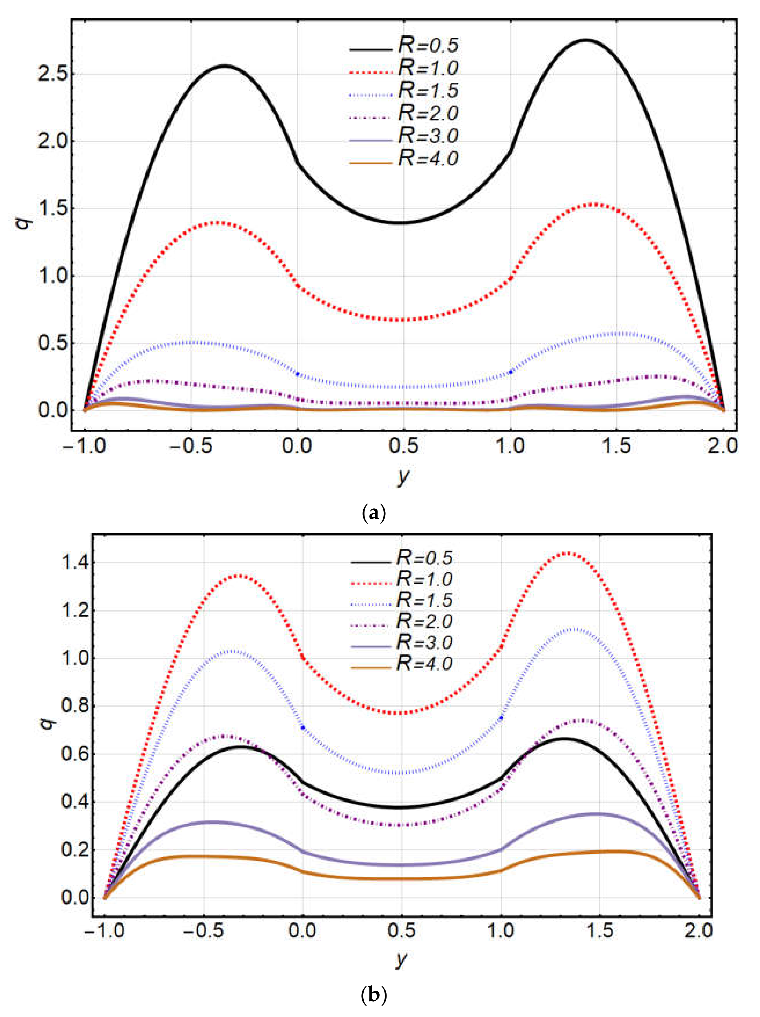
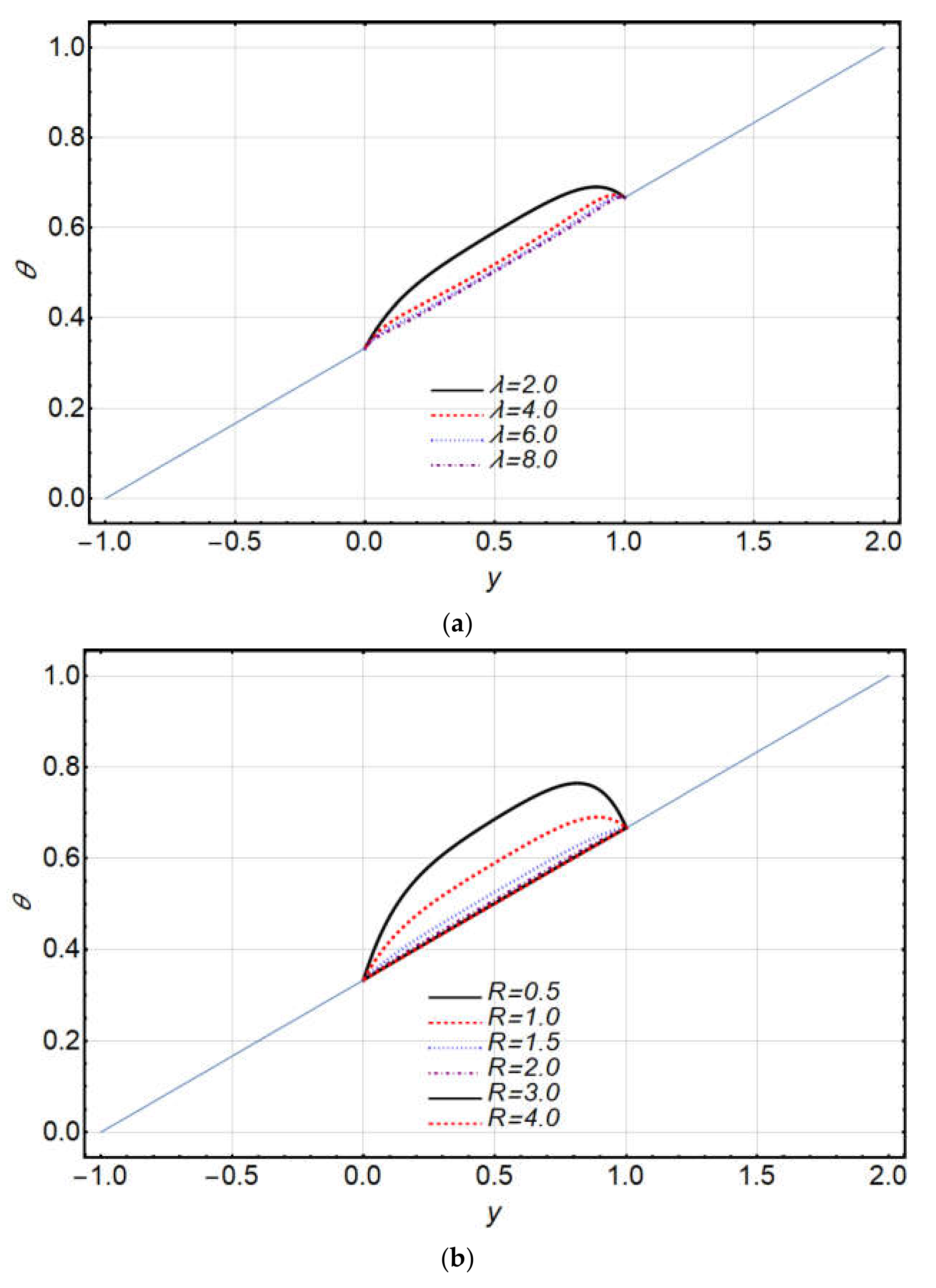
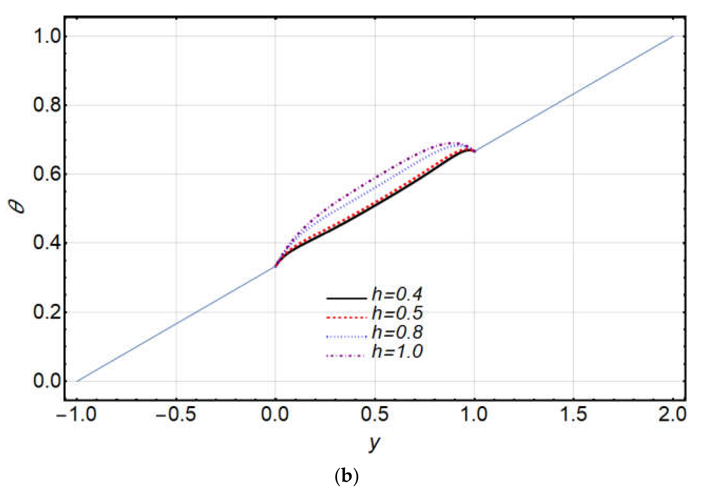
• Temperature distribution and both axial and transverse components of velocity decreased gradually for large values of the porous parameter $\lambda$ in all regions.
• Velocity components and temperature distribution slow down due to increasing rotation parameter $R$.
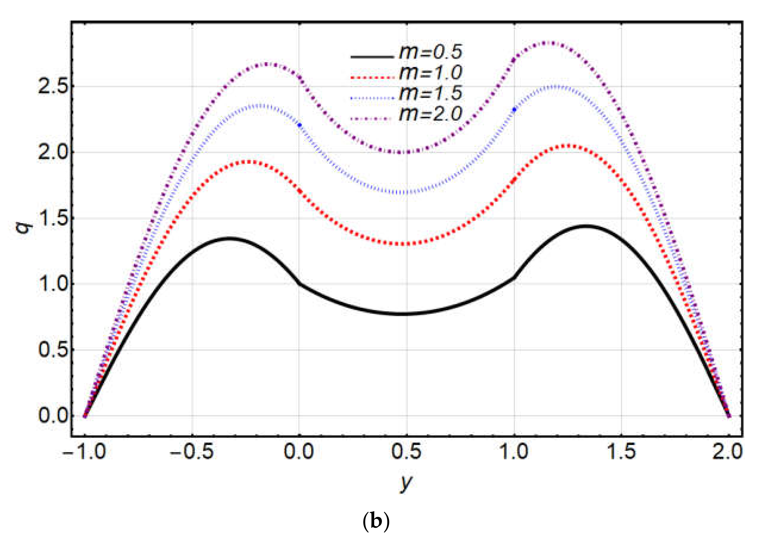
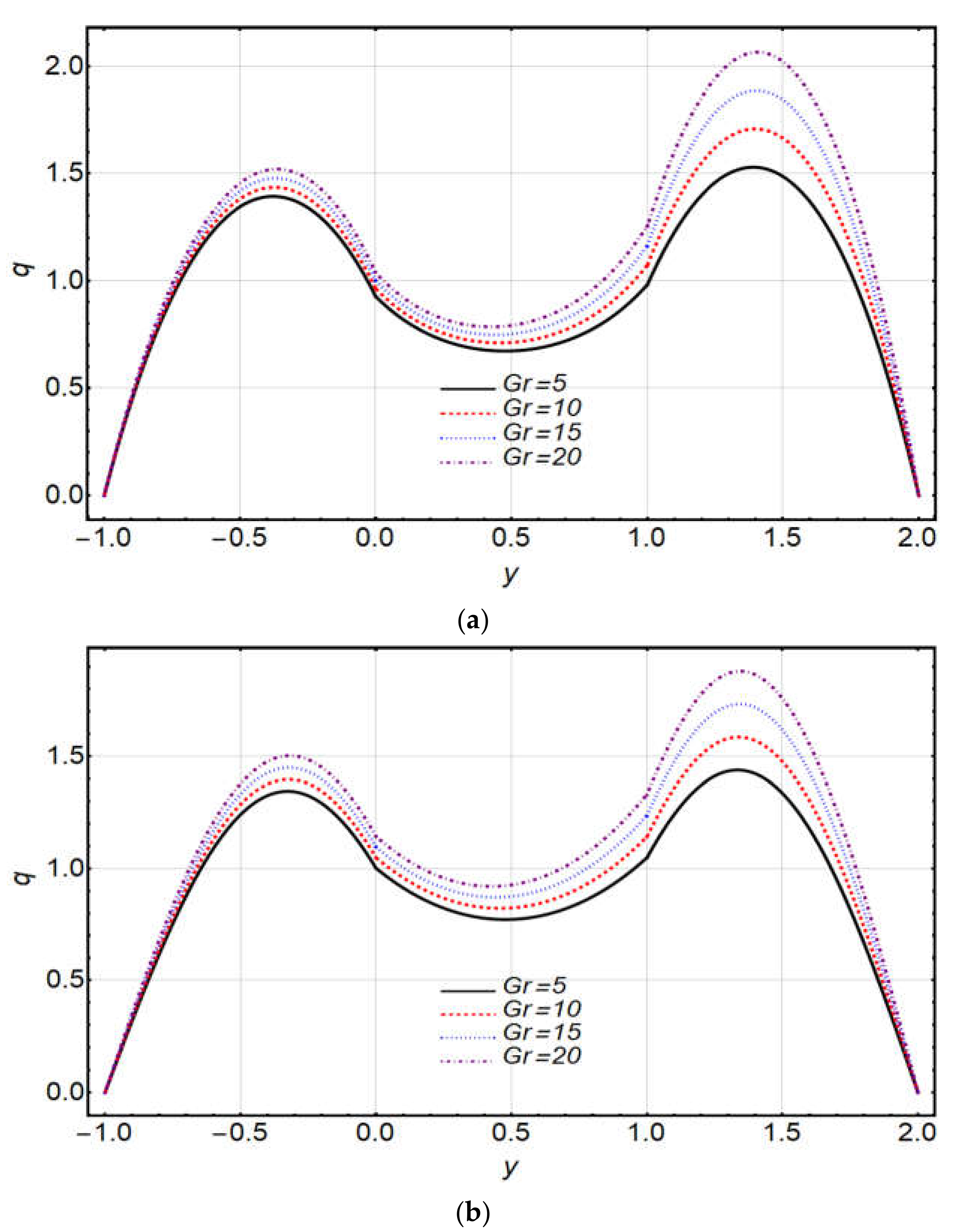
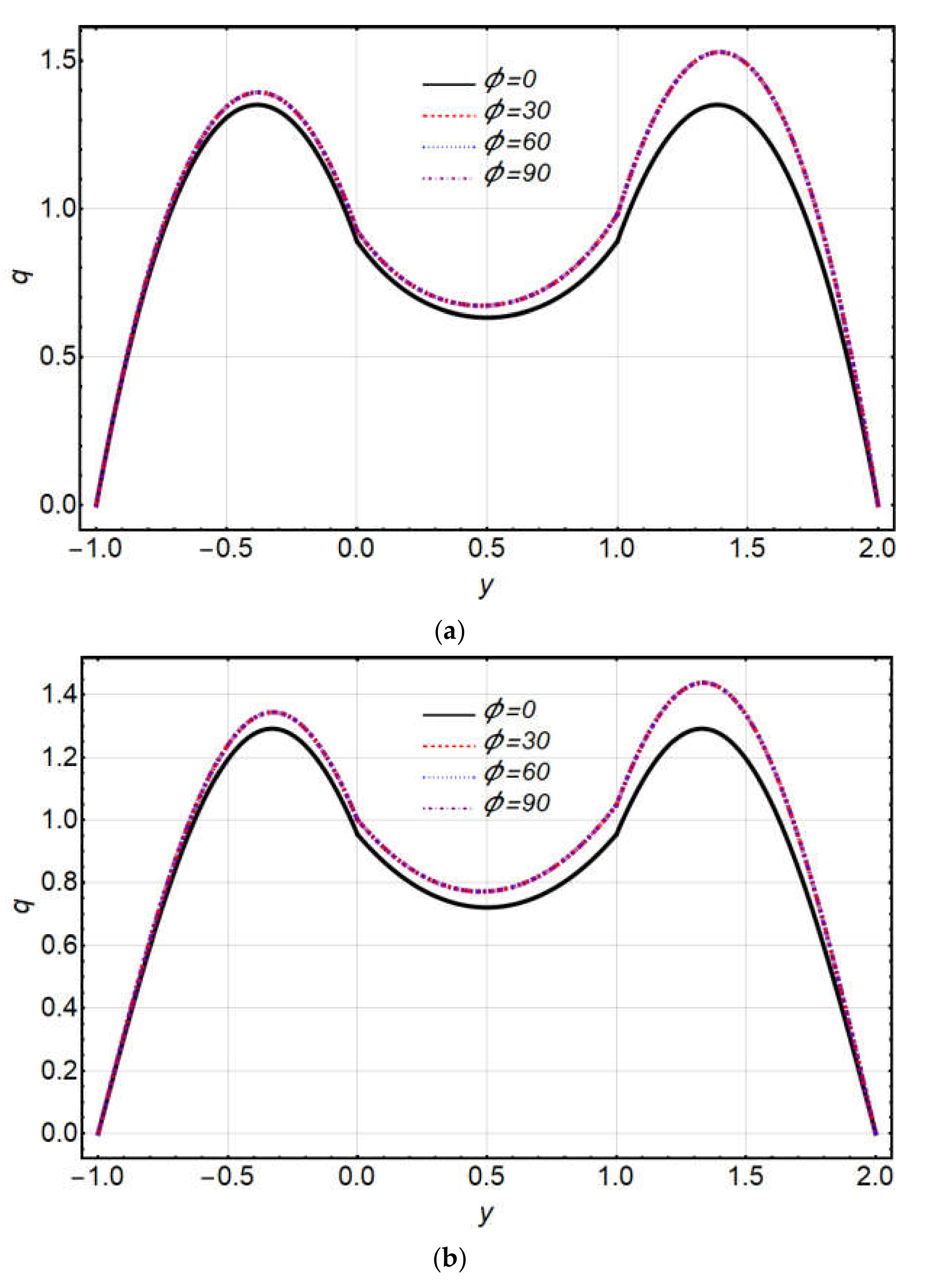
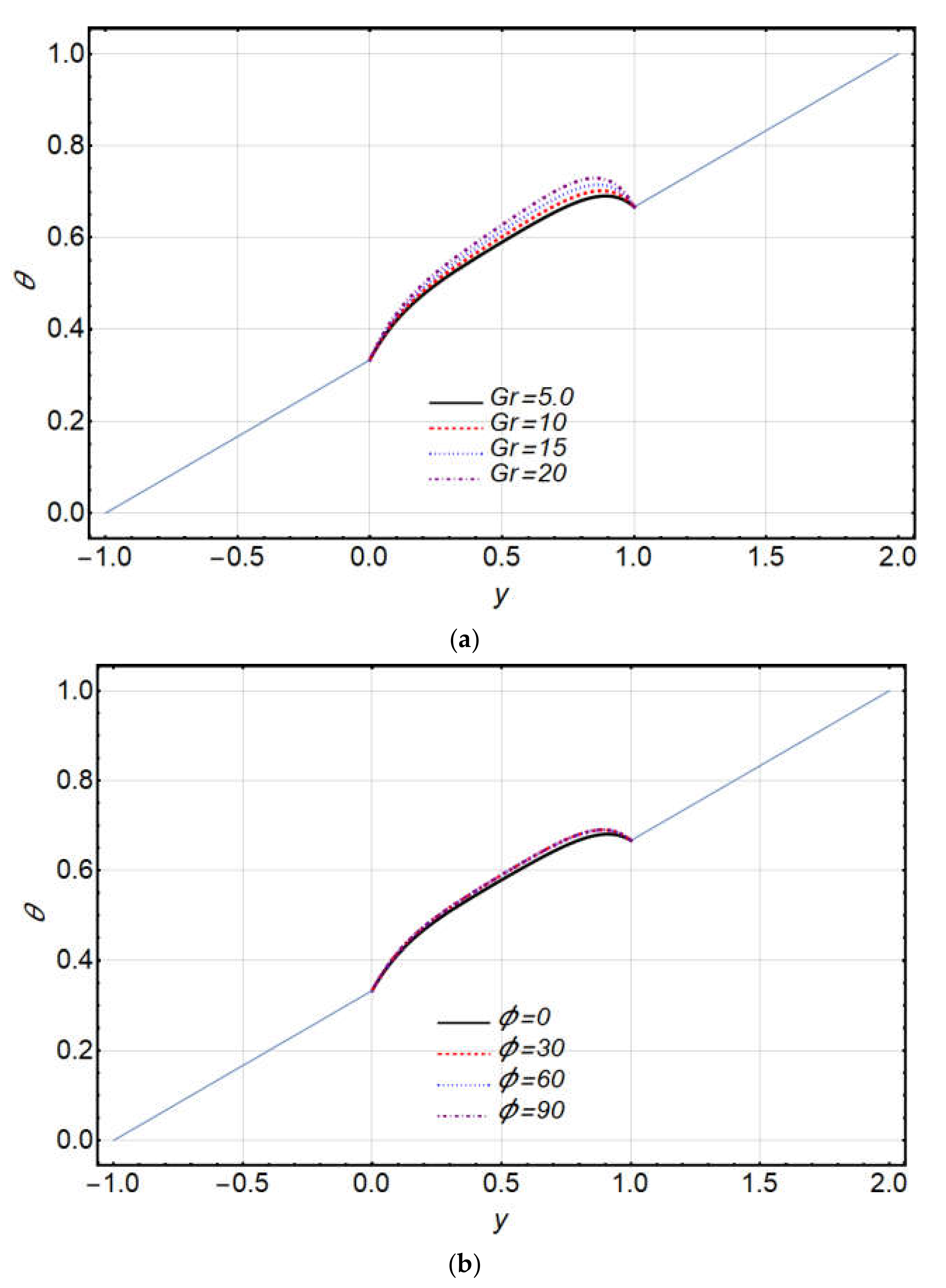
• Increases in the ratio of viscosities, Grashof number, and angle of inclination lead to increases in temperature and velocity components in all regions.
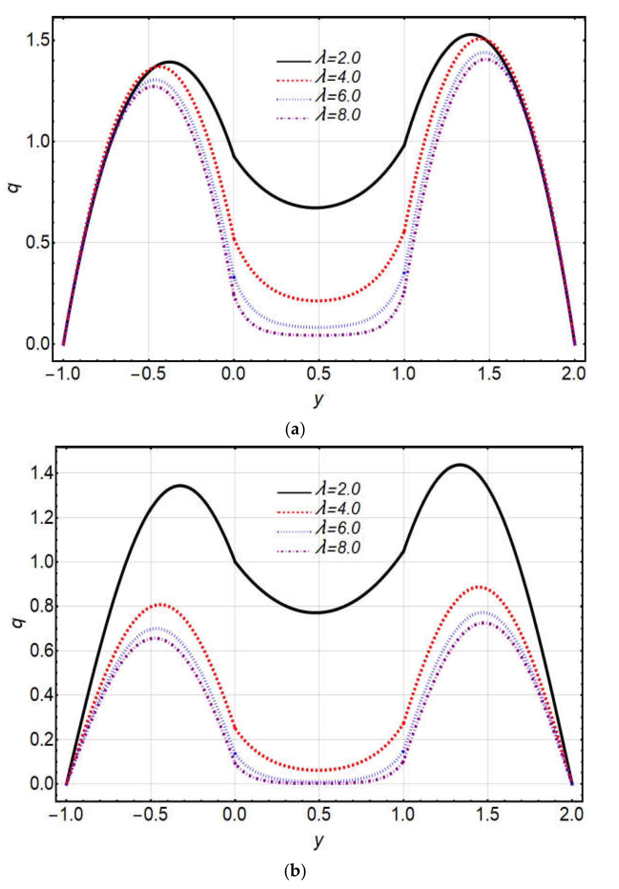
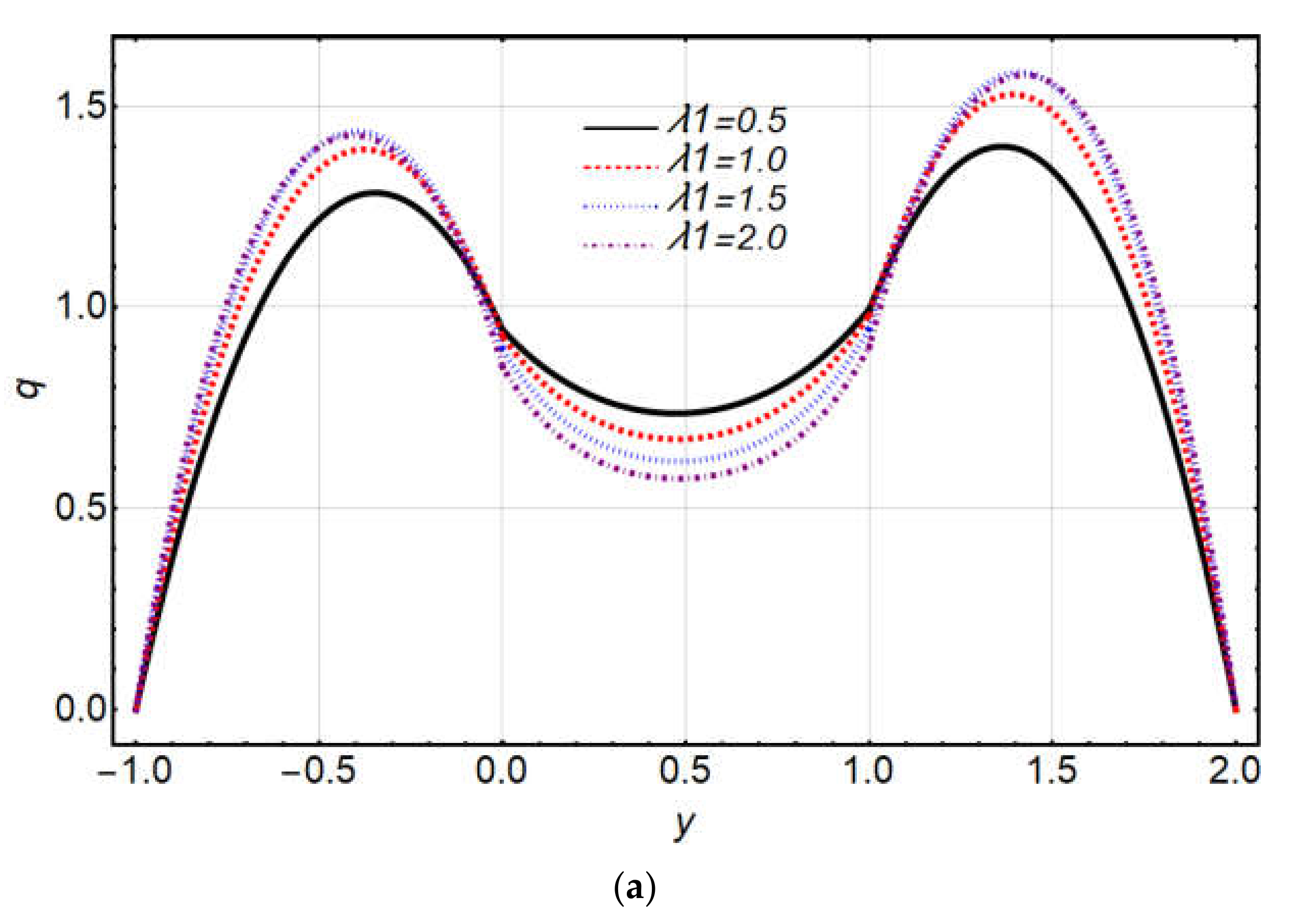
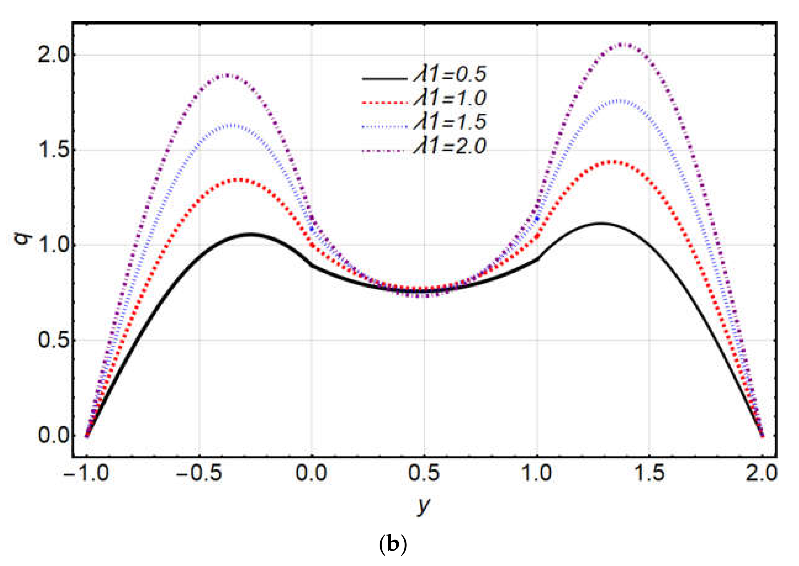
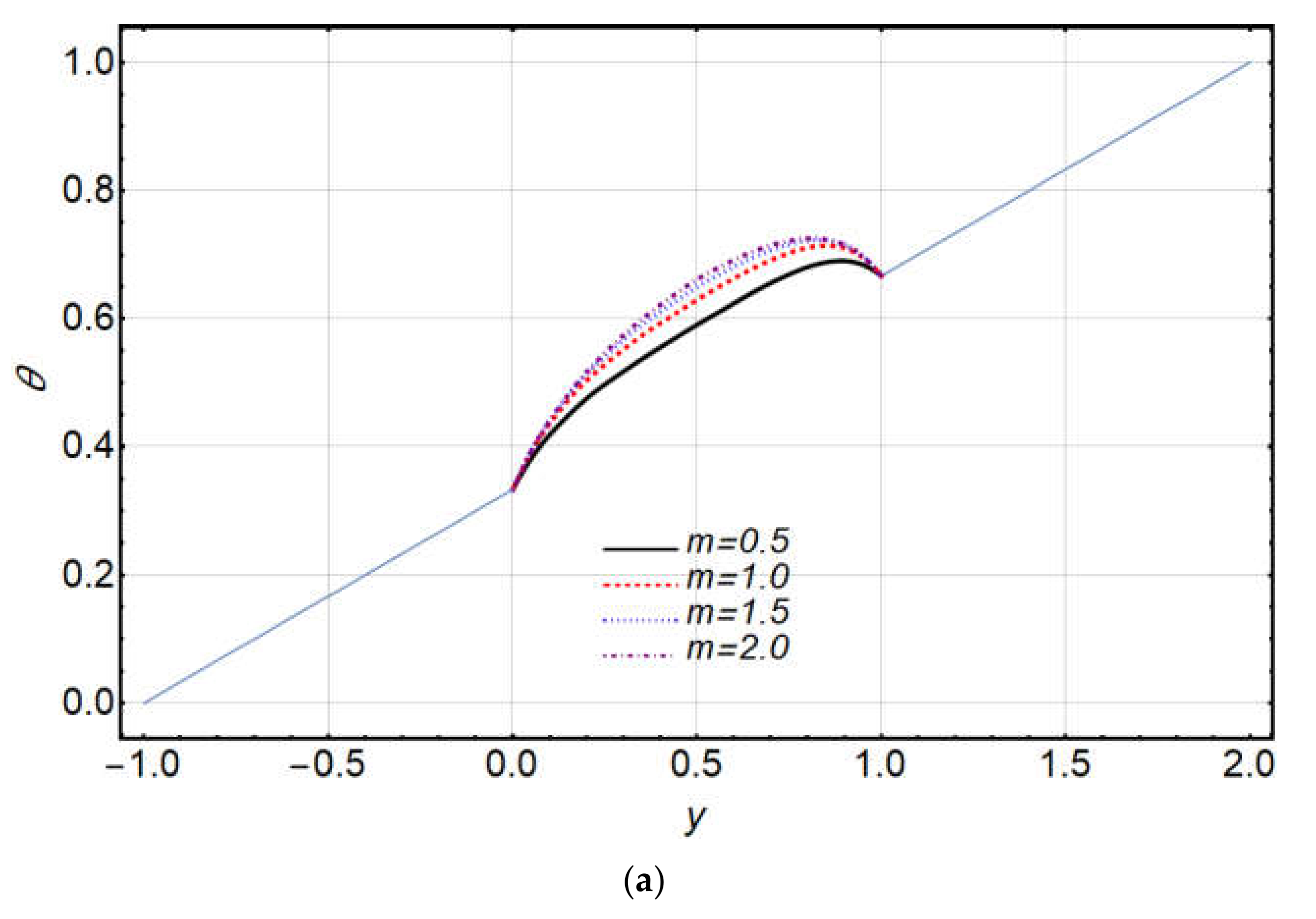
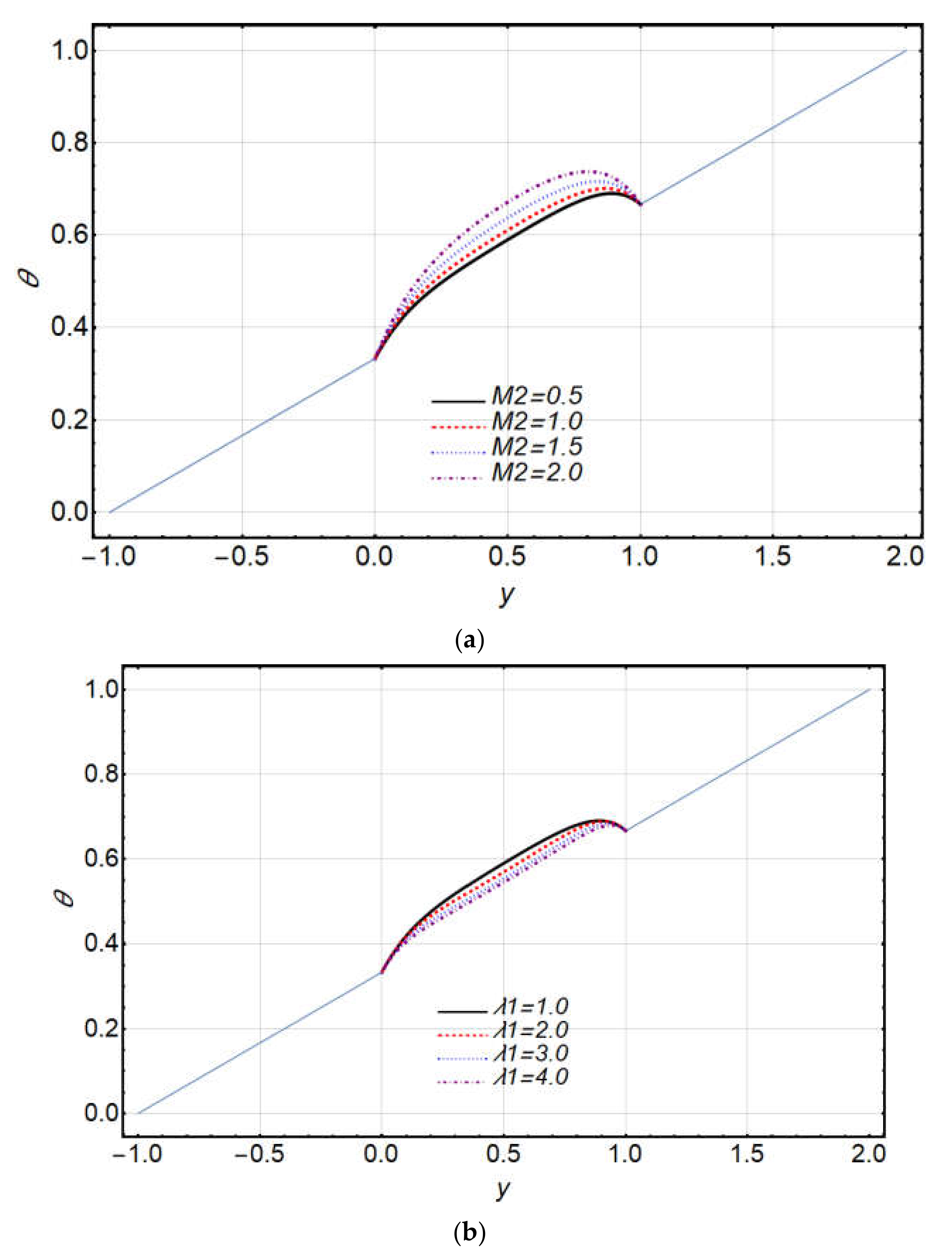
• The temperature distribution and both axial and transverse components of velocity increased thoroughly for the Jeffery parameter ${\lambda }_1$ in Region 2.
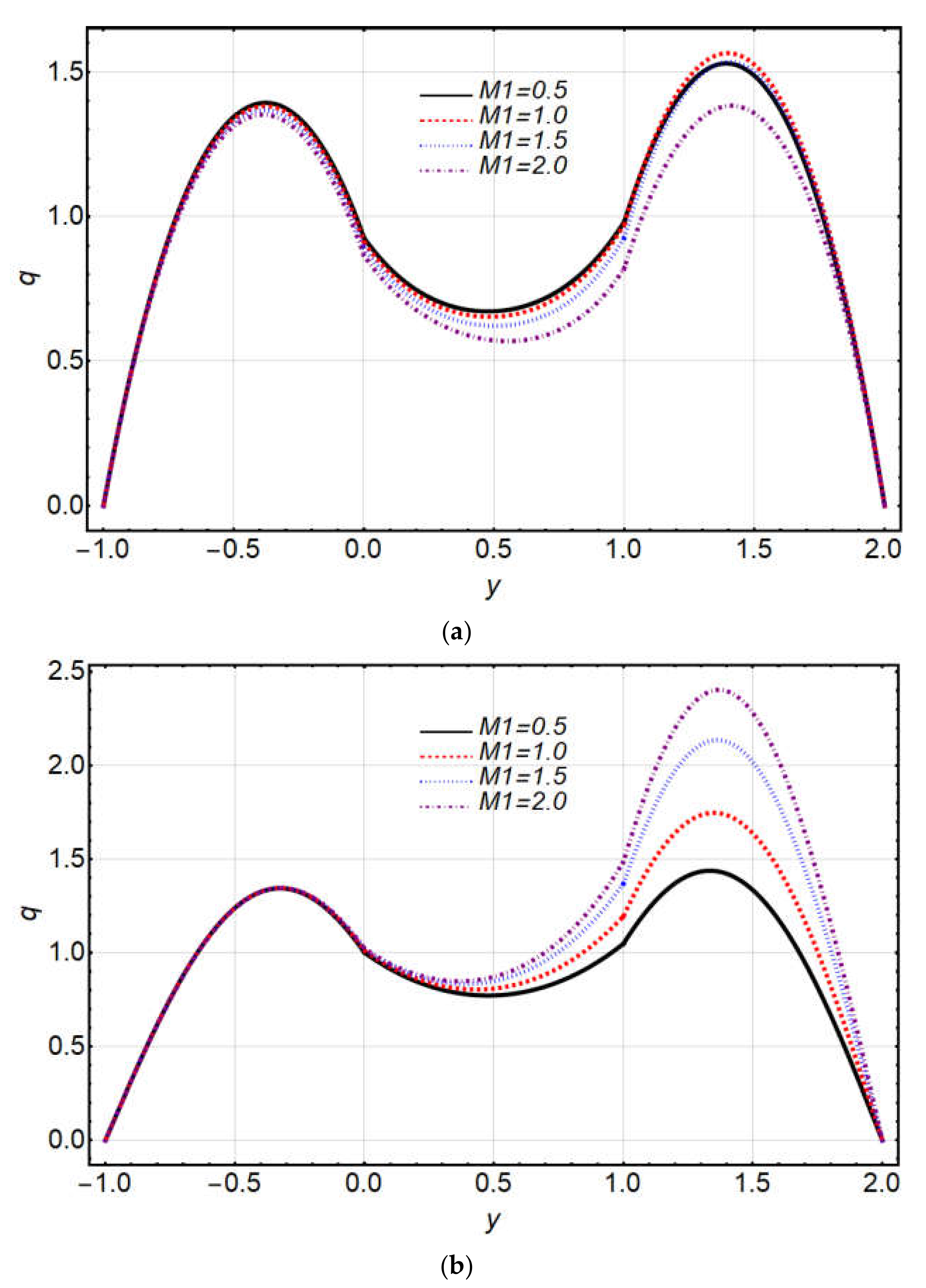
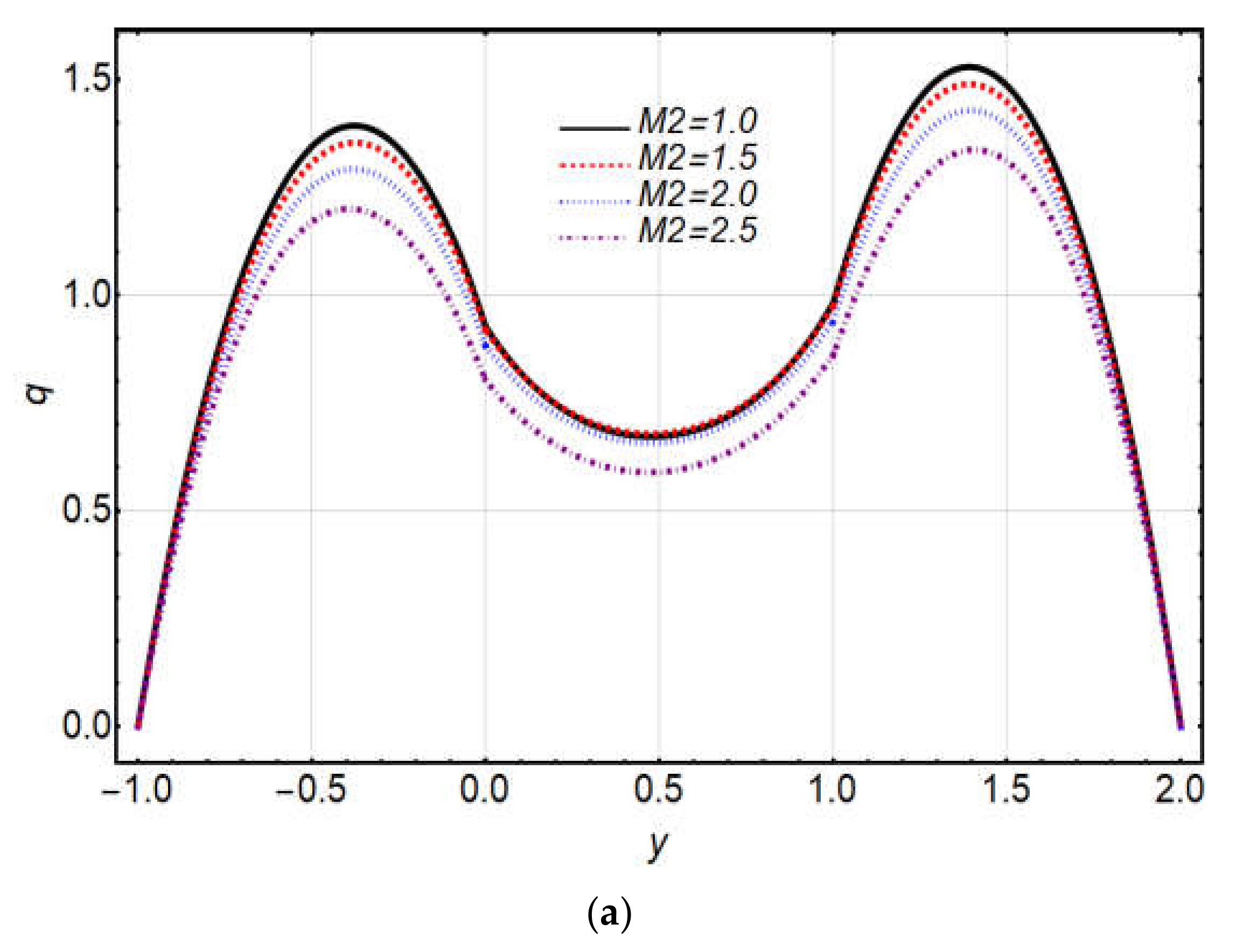
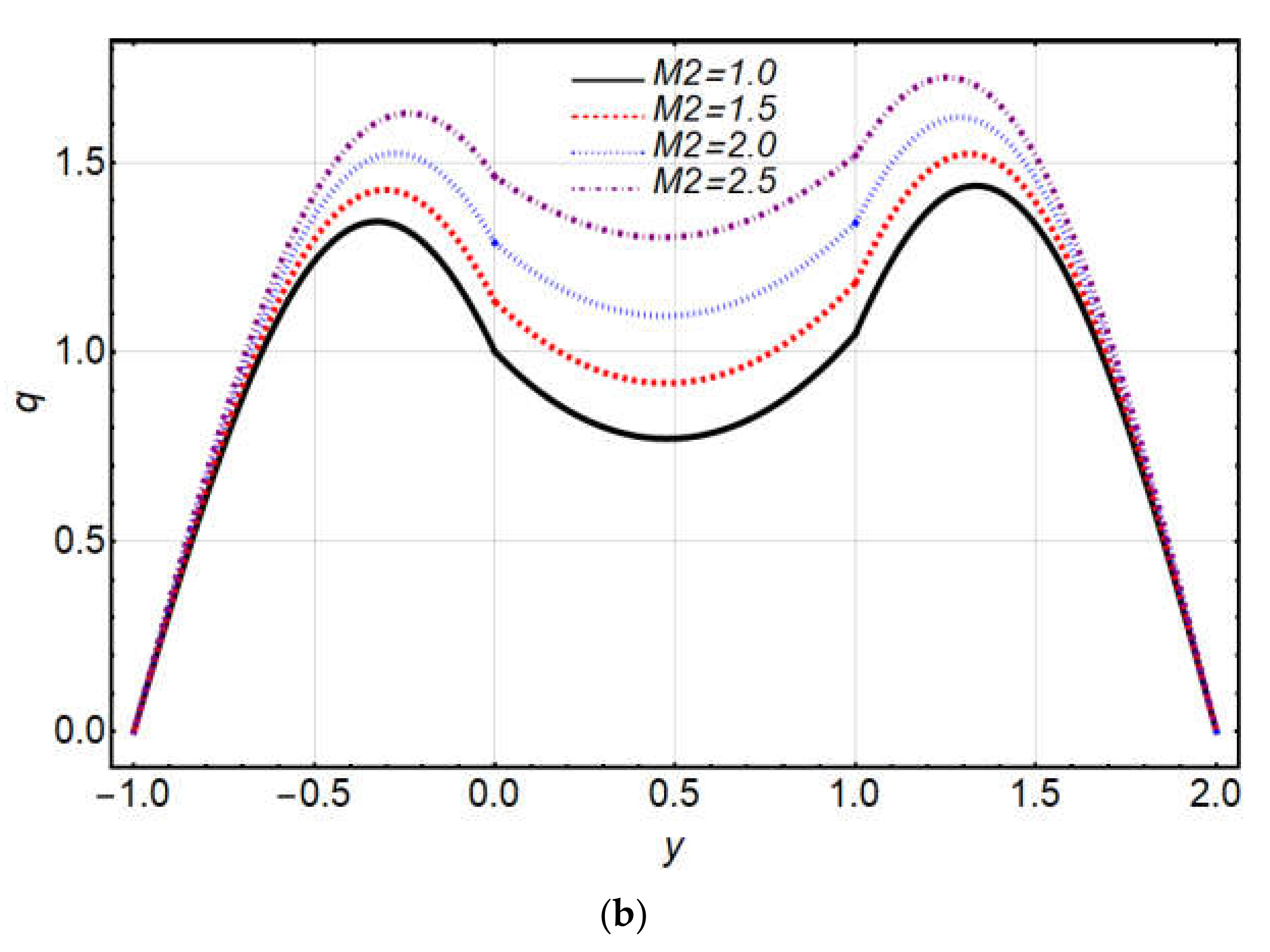
• The temperature rose due to the influence of magnetic field parameters and reduced velocity in all mediums. The reason behind this is drag force, which is initiated by magnetic fields in all regions.
• Heat transfer increased with the increasing values of the Jeffrey parameter.
• The magnetic field increased the magnitude of the Nusselt number at the bottom plate and decreased it at the top plate.

References

1. Akram, S.; Nadeem, S. Influence of induced magnetic field and heat transfer on the peristaltic motion of a Jeffrey fluid in an asymmetric channel: Closed-form solutions. J. Magn. Magn. Mater. 2013, 328, 11–20. [Google Scholar] [CrossRef]
2. Nallapu, S.; Radhakrishnamacharya, G. Jeffrey fluid flow through porous medium in the presence of magnetic field in narrow tubes. Int. J. Eng. Math. 2014, 2014, 713831. [Google Scholar] [CrossRef] [Green Version]
3. Abd-Alla, A.M.; Abo-Dahab, S.M.; Albalawi, M.M. Magnetic field and gravity effects on peristaltic transport of a Jeffrey fluid in an asymmetric channel. Abstr. Appl. Anal. 2014, 2014, 896121. [Google Scholar] [CrossRef]
4. Dhananjaya, S.; Arunachalam, P.V.; Sreenadh, S.; Parandhama, A. Free convection flow of a Jeffrey fluid between vertical plates partially filled with porous medium. Int. J. Sci. Res. Eng. Technol. 2015, 4, 503–512. [Google Scholar] [CrossRef] [Green Version]
5. Abd-Alla, A.M.; Abo-Dahab, S.M. Magnetic field and rotation effects on peristaltic transport of a Jeffrey fluid in an asymmetric channel. J. Magn. Magn. Mater. 2015, 374, 680–689. [Google Scholar] [CrossRef]
6. Murthy, M.K. MHD Couette flow of Jeffrey fluid in a porous channel with heat source and chemical reaction. Middle-East J. Sci. Res. 2016, 24, 585–592. [Google Scholar] [CrossRef]
7. Prakash, J.; Raju, C.S.K.; Sandeep, N. Dual solutions for heat and mass transfer in MHD Jeffrey fluid in the presence of homogeneous-heterogeneous reactions. Front. Heat Mass Transf. 2016, 7, 12431. [Google Scholar] [CrossRef] [Green Version]
8. Ellahi, R. Recent Trends in coatings and thin film: Modeling and application, coatings. Coatings 2020, 10, 777. [Google Scholar] [CrossRef]
9. Rashidi, M.M.; Erfani, E.; Bég, O.A.; Ghosh, S.K. Modified differential transform method (DTM) simulation of hydromagnetic multi-physical flow phenomena from a rotating disk. World J. Mech. 2011, 1, 217–230. [Google Scholar] [CrossRef] [Green Version]
10. Gomez, D.O.; Mininni, P.D. Direct numerical simulations of helical dynamo action: MHD and beyond. Nonlinear Proc. Geoph. 2004, 11, 619–629. [Google Scholar] [CrossRef] [Green Version]
11. Kumar, M.; Reddy, G.J.; Dalir, N. Transient entropy analysis of the magnetohydrodynamics flow of a Jeffrey fluid past an isothermal vertical flat plate. Pramana 2018, 91, 1–11. [Google Scholar] [CrossRef]
12. Graneau, P. Electrodynamic seawater jet: An alternative to the propeller. IEEE Trans. Magn. 1989, 25, 3275–3277. [Google Scholar] [CrossRef]
13. Romig, M.F. The influence of electric and magnetic fields on heat transfer to electrically conducting fluids. Adv. Heat Transf. 1964, 1, 267–354. [Google Scholar]
14. Rudraiah, N.; Kumudini, V.; Unno, W. Theory of nonlinear magnetoconvection and its application to solar convection problems. I., II. Publ. Astron. Soc. Jpn. 1985, 37, 183–233. [Google Scholar] [CrossRef]
15. Shail, R. On laminar two-phase flows in magnetohydrodynamics. Int. J. Eng. Sci. 1973, 11, 1103–1108. [Google Scholar] [CrossRef]
16. Lohrasbi, J.; Sahai, V. Magnetohydrodynamic heat transfer in two-phase flow between parallel plates. Appl. Sci. Res. 1988, 45, 53–66. [Google Scholar] [CrossRef]
17. Malashetty, M.S.; Leela, V. Magnetohydrodynamic Heat Transfer in Two-Fluid Flow. Proceeding of the National Heat Transfer Conference on AIChE and ASME HTD, Minneapolis, MN, USA, 26–31 July 1991; American Society of Mechanical Engineers: New York, NY, USA, 1991; p. 159. [Google Scholar]
18. Malashetty, M.S.; Leela, V. Magnetohydrodynamic heat transfer in two-phase flow. Int. J. Eng. Sci. 1992, 30, 371–377. [Google Scholar] [CrossRef]
19. Chauhan, D.S.; Rastogi, P. Hall current and heat transfer effects on MHD flow in a channel partially filled with a porous medium in a rotating system. Turk. J. Eng. Environ. Sci. 2010, 33, 167–184. [Google Scholar] [CrossRef]
20. Chauhan, D.S.; Rastogi, P. Heat transfer effects on rotating MHD Couette flow in a channel partially filled by a porous medium with Hall current. J. Appl. Sci. Eng. 2012, 15, 281–290. [Google Scholar] [CrossRef]
21. Seth, G.S.; Nandkeolyar, R.; Ansari, M.S. Hartmann flow in a rotating system in the presence of an inclined magnetic field with hall effects. J. Appl. Sci. Eng. 2010, 13, 243–252. [Google Scholar] [CrossRef]
22. Fiza, M.; Alsubie, A.; Ullah, H.; Hamadneh, N.N.; Islam, S.; Khan, I. Three-dimensional rotating flow of MHD Jeffrey fluid flow between two parallel plates with impact of hall current. Math. Probl. Eng. 2021, 2021, 6626411. [Google Scholar] [CrossRef]
23. Greenspan, H.P. The theory of rotating fluids: Cambridge monograph on mechanics and applied mathematics. Phys. Today 1969, 22, 81. [Google Scholar] [CrossRef]
24. Goodman, S. Radiant-heat transfer between nongray parallel plates. J. Res. Natl. Bur. Stand. 1957, 58, 37–40. [Google Scholar] [CrossRef]
25. Attia, H.A.; Kotb, N.A. MHD flow between two parallel plates with heat transfer. Acta Mech. 1996, 117, 215–220. [Google Scholar] [CrossRef]
26. Borkakoti, A.K.; Bharali, A. Hydromagnetic flow and heat transfer between two horizontal plates, the lower plate is a stretching sheet. Q. Appl. Math. 1983, 40, 461–467. [Google Scholar] [CrossRef] [Green Version]
27. Vajravelu, K.; Kumar, B.V.R. Analytical and numerical solutions of a coupled non-linear system arising in a three-dimensional rotating flow. Int. J. Non-Linear Mech. 2004, 39, 13–24. [Google Scholar] [CrossRef]
28. Das, S.K.; Choi, S.U.; Yu, W.; Pradeep, T. Nanofluids: Science and Technology; John Wiley & Sons: Hoboken, NJ, USA, 2007. [Google Scholar]
29. Mohyud-Din, S.T.; Zaidi, Z.A.; Khan, U.; Ahmed, N. On heat and mass transfer analysis for the flow of a nanofluid between rotating parallel plates. Aerosp. Sci. Technol. 2015, 46, 514–522. [Google Scholar] [CrossRef]
30. Murty, P.S.R.; Prakash, G.B. Heat transfer aspects on rotating MHD two-phase convective flow through an inclined channel in the presence of the electric field. Phys. Sci. Int. J. 2014, 2014, 1260–1279. [Google Scholar] [CrossRef]
31. Chitturi, K.S.; Paramsetti, S.R.M.; Kappala, S.B. Convective two-layered flow and temperature distribution through an inclined porous medium in a rotating system. J. Sci. Technol. 2020, 42, 371–382. [Google Scholar] [CrossRef]
32. Ijaz, N.; Riaz, A.; Zeeshan, A.; Ellahi, R.; Sait, S.M. Buoyancy driven flow with gas-liquid coatings of peristaltic bubbly flow in elastic walls. Coatings 2020, 10, 115. [Google Scholar] [CrossRef] [Green Version]
33. Ellahi, R.; Zeeshan, A.; Hussain, F.; Abbas, T. Thermally charged MHD bi-phase flow coatings with non-Newtonian nanofluid and hafnium particles along slippery walls. Coatings 2019, 9, 300. [Google Scholar] [CrossRef] [Green Version]
34. Asadollahi, A.; Esfahani, J.A.; Ellahi, R. Evacuating liquid coatings from a diffusive oblique fin in micro-/mini-channels. J. Therm. Anal. Calorim. 2019, 138, 255–263. [Google Scholar] [CrossRef]
35. Ellahi, R.; Zeeshan, A.; Hussain, F.; Abbas, T. Study of shiny film coating on multi-fluid flows of a rotating disk suspended with nano-sized silver and gold particles: A comparative analysis. Coatings 2018, 8, 422. [Google Scholar] [CrossRef] [Green Version]
36. Ur Rasheed, H.; AL-Zubaidi, A.; Islam, S.; Saleem, S.; Khan, Z.; Khan, W. Effects of Joule heating and viscous dissipation on magnetohydrodynamic boundary layer flow of Jeffrey nanofluid over a vertically stretching cylinder. Coatings 2021, 11, 353. [Google Scholar] [CrossRef]
37. Ramzan, M.; Liaquat, A.; Kadry, S.; Yu, S.; Nam, Y.; Lu, D. Impact of second-order slip and double stratification coatings on 3d MHD Williamson nanofluid flow with Cattaneo–Christof heat flux. Coatings 2019, 9, 849. [Google Scholar] [CrossRef] [Green Version]
38. Vajravelu, K.; Sreenadh, S.; Lakshminarayana, P. The influence of heat transfer on peristaltic transport of a Jeffrey fluid in a vertical porous stratum. Commun. Nonlinear Sci. Numer. Simul. 2011, 16, 3107–3125. [Google Scholar] [CrossRef]
Figure 1. Physical configuration.
Coatings 12 00430 g001
Figure 2. Velocity distribution against λ : (a) axial, (b) transverse.
Coatings 12 00430 g002
Figure 3. Velocity distribution of h : (a) axial, (b) transverse.
Coatings 12 00430 g003
Figure 4. Velocity distribution of m : (a) axial, (b) transverse.
Coatings 12 00430 g004aCoatings 12 00430 g004b
Figure 5. Velocity distribution of G r : (a) axial, (b) transverse.
Coatings 12 00430 g005
Figure 6. Velocity distribution of ϕ : (a) axial, (b) transverse.
Coatings 12 00430 g006
Figure 7. Velocity distribution of λ 1 : (a) axial, (b) transverse.
Coatings 12 00430 g007aCoatings 12 00430 g007b
Figure 8. Velocity distribution of R : (a) axial, (b) transverse.
Coatings 12 00430 g008
Figure 9. Velocity distribution of M 1 : (a) axial, (b) transverse.
Coatings 12 00430 g009
Figure 10. Velocity distribution of M 2 : (a) axial, (b) transverse.
Coatings 12 00430 g010aCoatings 12 00430 g010b
Figure 11. Temperature distribution against (a) λ , (b) R .
Coatings 12 00430 g011
Figure 12. Temperature distribution against (a) G r , (b) ϕ .
Coatings 12 00430 g012
Figure 13. Temperature distribution against (a) m , (b) h .
Coatings 12 00430 g013aCoatings 12 00430 g013b
Figure 14. Temperature distribution against (a) M 2 , (b) λ 1 .
Coatings 12 00430 g014