Response of Coccomyxa cimbrica sp.nov. to Increasing Doses of Cu(II) as a Function of Time: Comparison between Exposure in a Microfluidic Device or with Standard Protocols

 ,
,  and
and 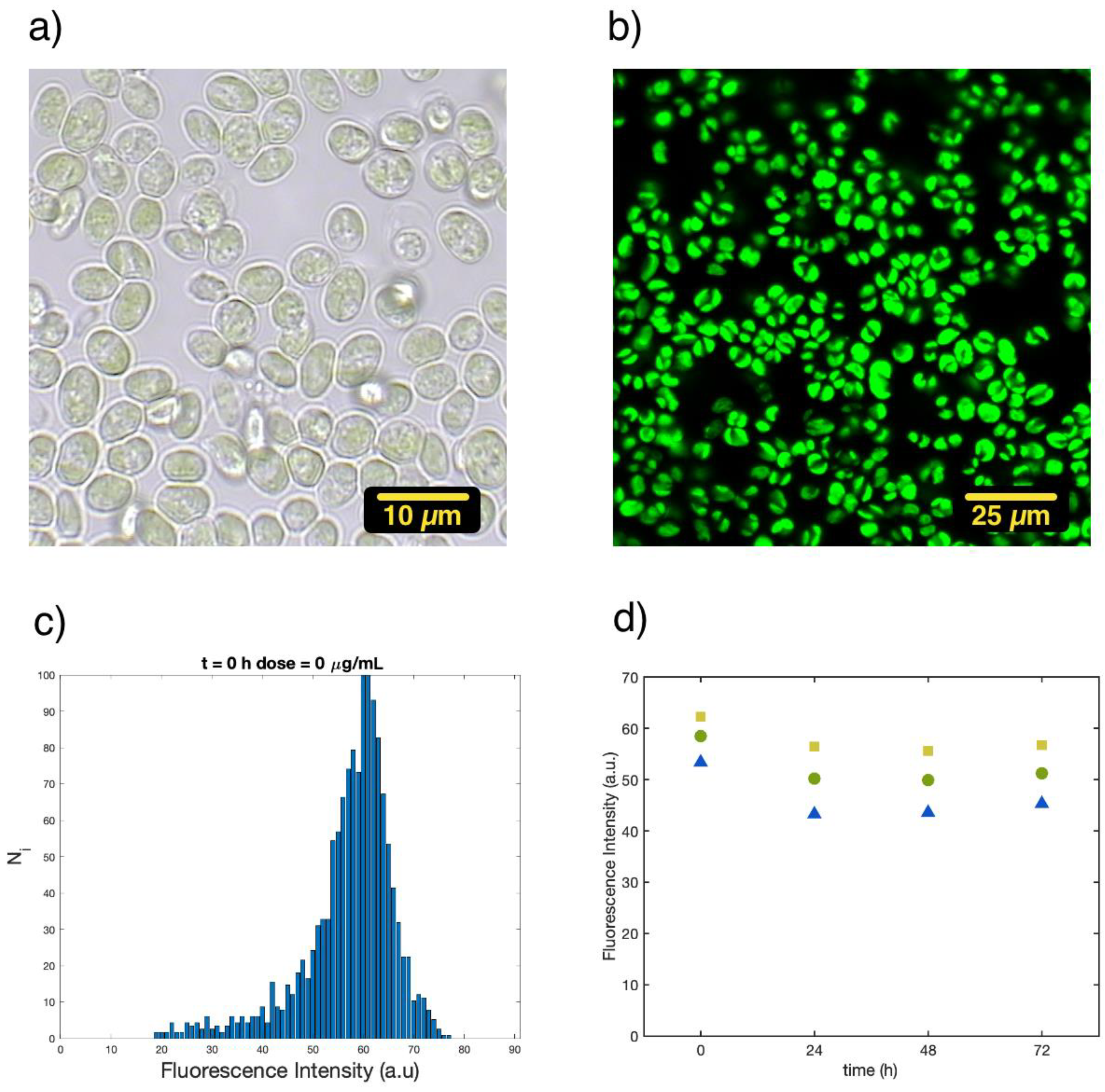
Abstract
:1. Introduction
2. Materials and Methods
3. Results and Discussion
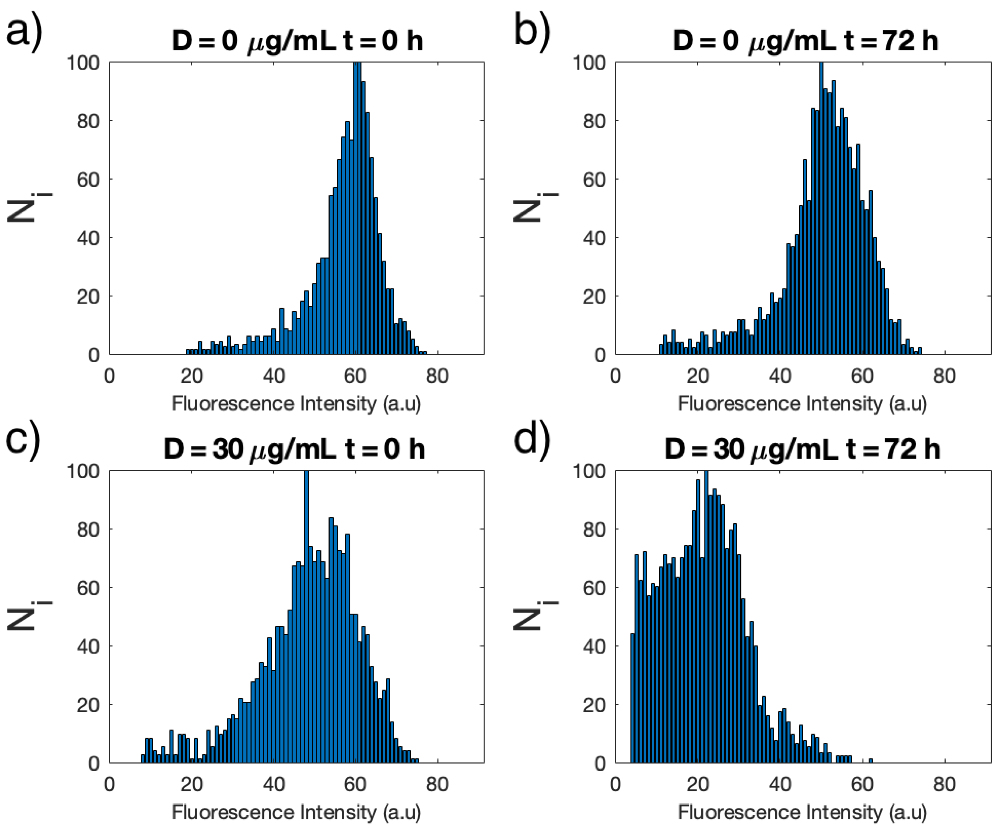
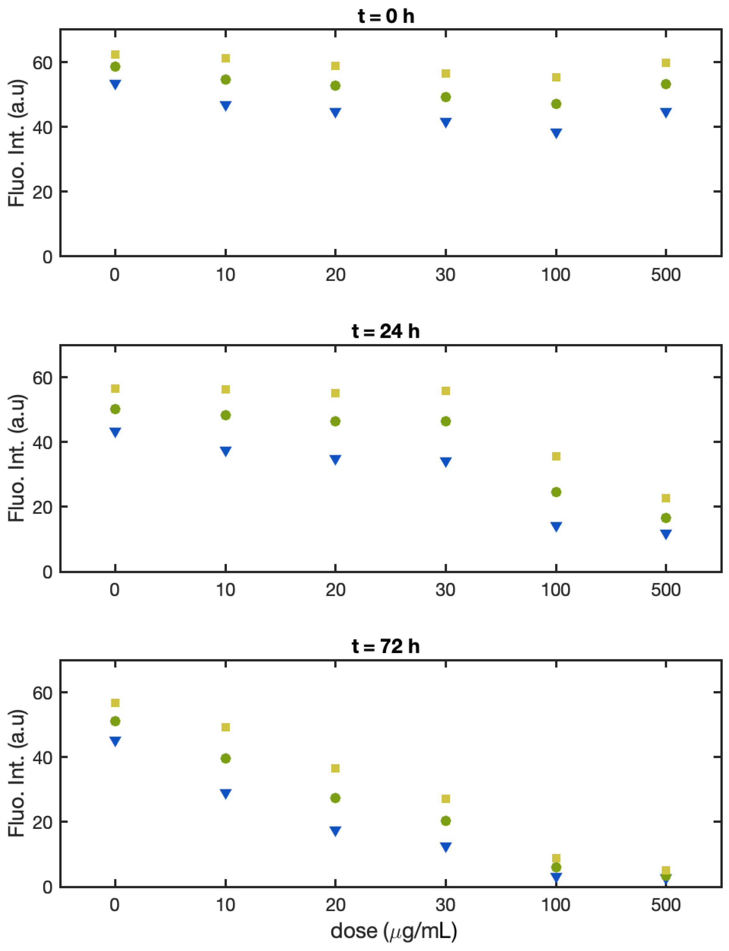
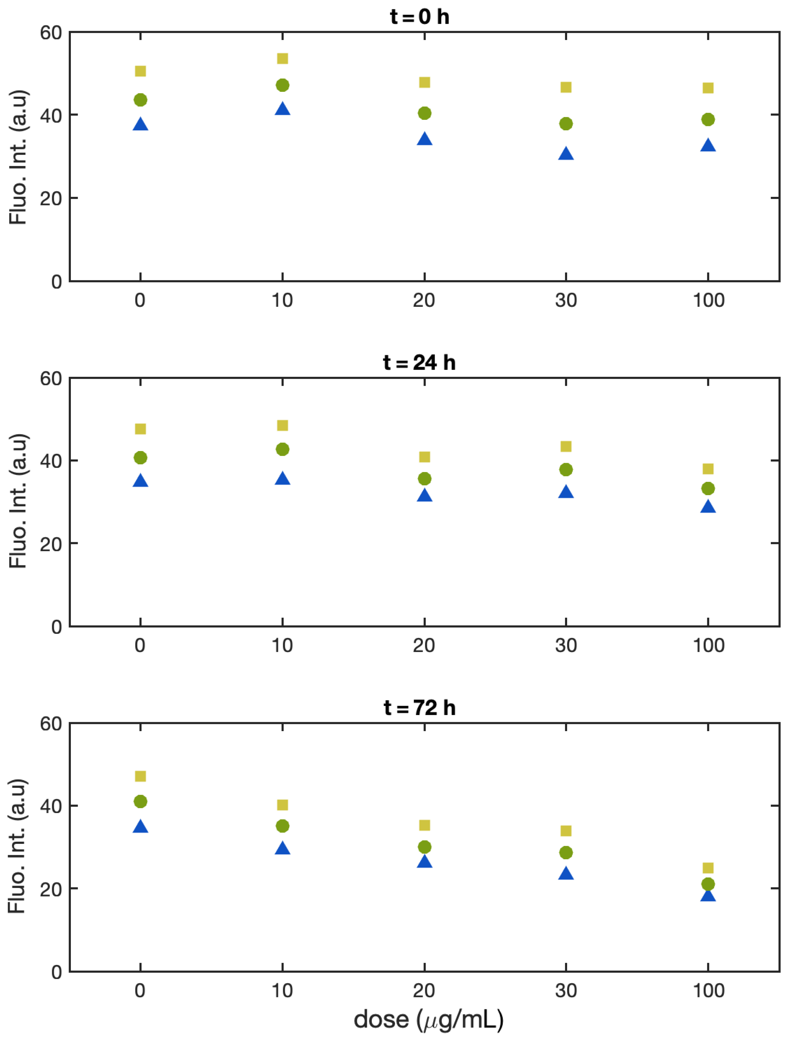
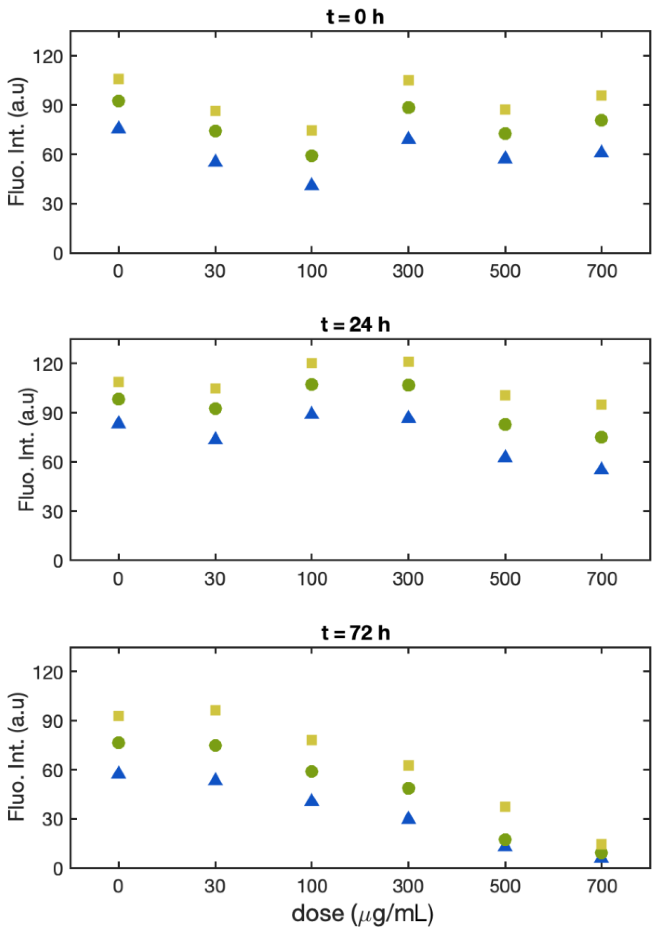
3.1. Single-Cell Fluorescence Intensity Imaging
- Batch 1:
- Batch 2:
- Batch 3:
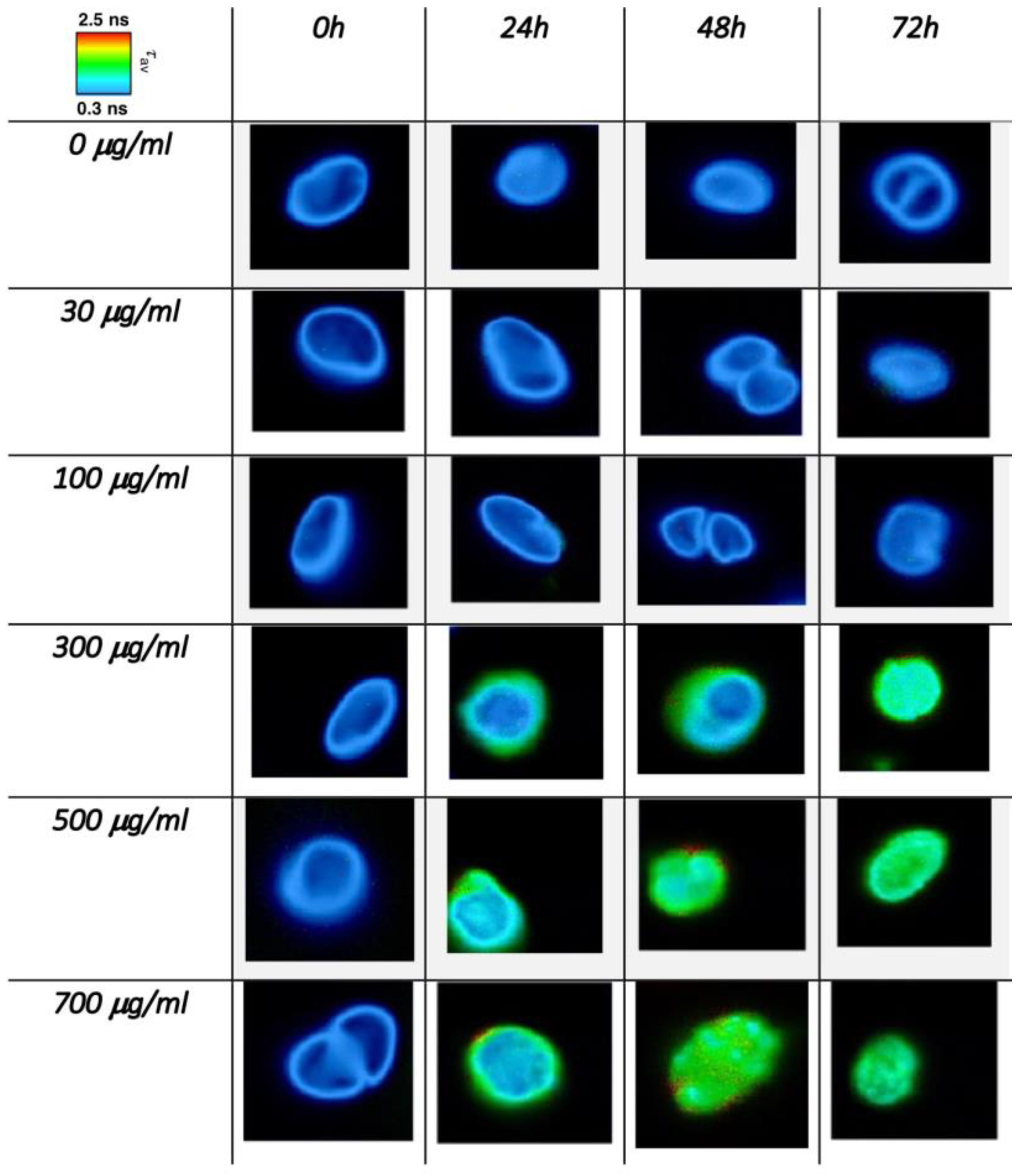
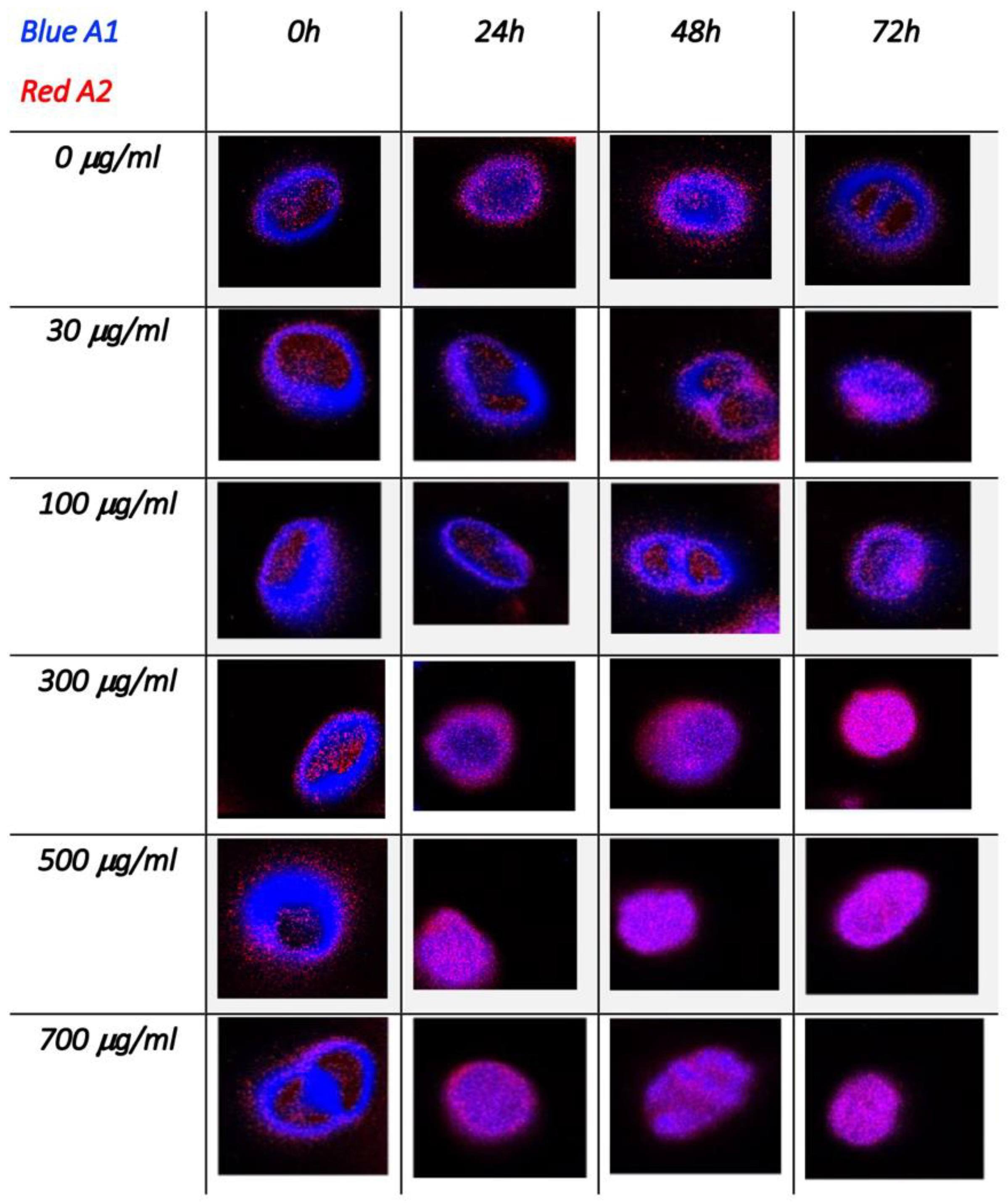
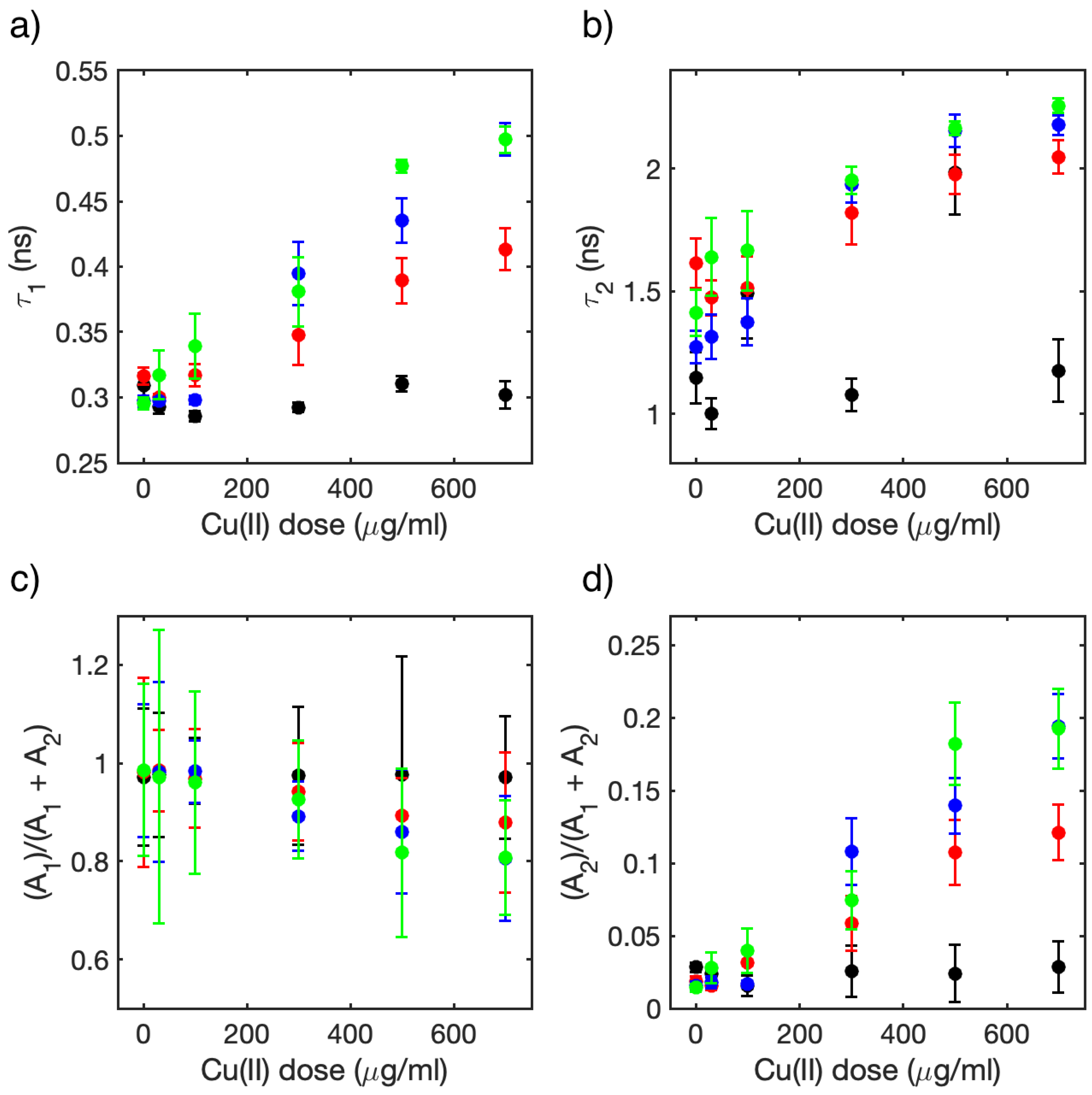
3.2. Single-Cell FLIM Experiments
4. Conclusions
Supplementary Materials
Author Contributions
Funding
Data Availability Statement
Conflicts of Interest
References
- Chisti, Y. Biodiesel from microalgae. Biotechnol. Adv. 2007, 25, 294–306. [Google Scholar] [CrossRef]
- Muñoz, R.; Guieysse, B. Algal–bacterial processes for the treatment of hazardous contaminants: A review. Water Res. 2006, 30, 2799–2815. [Google Scholar] [CrossRef]
- Kumar, H.S.; Dahm, H.-U.; Lee, J.-S.; Kim, H.C.; Lee, W.C.; Shin, H.-H. Algal photosynthetic responses to toxic metals and herbicides assessed by chlorophyll a fluorescence. Ecotoxicol. Environ. Saf. 2014, 104, 51–71. [Google Scholar] [CrossRef] [PubMed]
- Maxwell, K.; Johnson, G.N. Chlorophyll fluorescence—A practical guide. J. Exp. Bot. 2000, 51, 659–668. [Google Scholar] [CrossRef] [PubMed]
- Rocchetta, I.; Küpper, H. Chromium- and copper-induced inhibition of photosynthesis in Euglena gracilis analysed on the single-cell level by fluorescence kinetic microscopy. New Phytol. 2009, 182, 405–420. [Google Scholar] [CrossRef] [Green Version]
- Lombardi, A.T.; Maldonado, M.T. The effects of copper on the photosynthetic response of Phaeocystis cordata. Photosynth. Res. 2011, 108, 77–87. [Google Scholar] [CrossRef] [PubMed]
- Rocha, G.S.; Parrish, C.C.; Espíndola, E.L.G. Effects of copper on photosynthetic and physiological parameters of a freshwater microalga (Chlorophyceae). Algal Res. 2021, 54, 102223. [Google Scholar] [CrossRef]
- Franklin, N.M.; Stauber, J.L.; Lim, R.P. Development of flow cytometry-based algal bioassays for assessing toxicity of copper in natural waters. Environ. Toxicol. Chem. Int. J. 2001, 20, 160–170. [Google Scholar] [CrossRef]
- Franquiera, D.; Orosa, M.; Torres, E.; Herrero, C.; Cid, A. Potential use of flow cytometry in toxicity studies with microalgae. Sci. Total Environ. 2000, 247, 119–126. [Google Scholar] [CrossRef] [Green Version]
- Bastiaens, P.I.H.; Squire, A. Fluorescence lifetime imaging microscopy: Spatial resolution of biochemical processes in the cell. Trends Cell Biol. 1999, 9, 48–52. [Google Scholar] [CrossRef]
- Borst, J.W.; Wisser, A.J.W.G. Fluorescence lifetime imaging microscopy in life sciences. Meas. Sci. Technol. 2010, 21, 102002. [Google Scholar] [CrossRef]
- Nozoue, S.; Mukuno, A.; Tsuda, Y.; Shiina, T.; Terazima, M.; Kumazaki, S.; Nozue, S.; Mukuno, A.; Tsuda, Y.; Shiina, T.; et al. Characterization of thylakoid membrane in a heterocystous cyanobacterium and green alga with dual-detector fluorescence lifetime imaging microscopy with a systematic change of incident laser power. Biochim. Biophys. Acta 2016, 1857, 46–59. [Google Scholar] [CrossRef] [PubMed] [Green Version]
- Broess, K.; Borst, J.W.; van Amerongen, H. Applying two-photon excitation fluorescence lifetime imaging microscopy to study photosynthesis in plant leaves. Photosynth. Res. 2009, 100, 89–96. [Google Scholar] [CrossRef] [Green Version]
- Iermak, I.; Vink, J.; Bader, A.N.; Wientjes, E.; van Amerongen, H. Visualizing heterogeneity of photosynthetic properties of plant leaves with two-photon fluorescence lifetime imaging microscopy. Biochim. Biophys. Acta 2016, 1857, 1473–1478. [Google Scholar] [CrossRef] [PubMed]
- Chorvatova, A.M.; Uherek, A.M.; Chorvat, D. Biosensing the Presence of Metal Nanoparticles by Spectrally- and Time-Resolved Endogenous Fluorescence in Water Moss Fontinalis antipyretica. Front. Phys. 2021, 9, 634324. [Google Scholar] [CrossRef]
- Hötzer, B.; Ivanov, R.; Brumbarova, T.; Bauer, P.; Jung, G. Visualization of Cu2+ uptake and release in plant cells by fluorescence lifetime imaging microscopy. FEBS J. 2012, 279, 410–419. [Google Scholar] [CrossRef] [PubMed]
- Shin, J.H.; Choi, S. Open-source and do-it-yourself microfluidics. Sens. Actuators B Chem. 2021, 347, 130624. [Google Scholar] [CrossRef]
- El-Ali, J.; Sorger, P.K.; Jensen, K.F. Cells on chips. Nature 2006, 442, 403–411. [Google Scholar] [CrossRef] [PubMed]
- Tsai, T.H.-F.; Trubelja, A.; Shen, A.Q.; Bao, G. Tumour-on-a-chip: Microfluidic models of tumour morphology, growth and microenvironment. J. R. Soc. Interface 2017, 14, 20170137. [Google Scholar] [CrossRef] [Green Version]
- Yeo, L.Y.; Chang, H.-C.; Chan, P.P.Y.; Friend, J.R. Microfluidic Devices for Bioapplications. Small 2011, 7, 12–48. [Google Scholar] [CrossRef]
- Kim, H.S.; Devarenne, T.P.; Han, A.; Kim, H.S.; Devarenne, T.P.; Han, A. Microfluidic systems for microalgal biotechnology: A review. Algal Res. 2018, 30, 149–161. [Google Scholar] [CrossRef]
- Zheng, X.; Duan, X.; Tu, X.; Jiang, S.; Song, C. The fusion of microfluidics and optics for on-chip detection and characterization of microalgae. Micromachines 2021, 12, 1137. [Google Scholar] [CrossRef] [PubMed]
- Benazzi, G.; Holmes, D.; Sun, T.; Mowlem, M.V.; Morgan, H. Discrimination and analysis of phytoplankton using a microfluidic cytometer. IET Nanobiotechnnol. 2007, 1, 94–101. [Google Scholar] [CrossRef] [PubMed]
- Deng, Y.L.; Chang, J.S.; Juang, Y.J. Separation of microalgae with different lipid contents by dielectrophoresis. Bioresour. Technol. 2013, 135, 137–141. [Google Scholar] [CrossRef]
- Deng, Y.L.; Kuo, M.Y.; Juang, Y.J. Development of flow through dielectrophoresis microfluidic chips for biofuel production: Sorting and detection of microalgae with different lipid contents. Biomicrofluidics 2014, 8, 064120. [Google Scholar] [CrossRef] [Green Version]
- Lim, H.S.; Kim, J.Y.H.; Kwak, H.S.; Sim, S.J. Integrated microfluidic platform for multiple processes from microalgal culture to lipid extraction. Anal. Chem. 2014, 86, 8585–8592. [Google Scholar] [CrossRef]
- Chen, M.; Mertiri, T.; Holland, T.; Basu, A.S. Optical microplates for high-throughput screening of photosynthesis in lipid-producing algae. Lab Chip 2012, 12, 3870–3874. [Google Scholar] [CrossRef]
- Dewan, A.; Kim, J.; McLean, R.H.; Vanapalli, S.A.; Karim Dewan, M.N. Growth kinetics of microalgae in microfluidic static droplet arrays. Biotechnol. Bioeng. 2012, 109, 2987–2996. [Google Scholar] [CrossRef]
- Kim, H.S.; Guzman, A.R.; Thapa, H.R.; Devarenne, T.P.; Han, A. A droplet microfluidics platform for rapid microalgal growth and oil production analysis. Biotech. Bioeng. 2016, 113, 1691–1701. [Google Scholar] [CrossRef]
- Zheng, G.-X.; Li, Y.-J.; Qi, L.-L.; Liu, X.-M.; Wang, H.; Yu, S.-P.; Wang, Y.-H. Marine phytoplankton motility sensor integrated into a microfluidic chip for high-throughput pollutant toxicity assessment. Mar. Pollut. Bul. 2014, 84, 147–154. [Google Scholar] [CrossRef]
- Han, S.; Zhang, Q.; Zhang, X.; Liu, X.; Lu, L.; Wei, J.; Li, Y.; Wang, Y.; Zheng, G. A digital microfluidic diluter-based microalgal motion biosensor for marine pollution monitoring. Biosens. Bioelectron. 2019, 143, 111597. [Google Scholar] [CrossRef] [PubMed]
- Lefèvre, F.; Chalifour, A.; Yu, L.; Chadovarapu, V.; Juneau, P.; Izquierdo, R. Algal fluorescence sensor integrated into a microfluidic chip for water pollutant detection. Lab Chip 2012, 12, 787–793. [Google Scholar] [CrossRef] [PubMed]
- Kürsten, D.; Cao, J.; Funfak, A.; Müller, P.; Köhler, J.M. Cultivation of Chlorella vulgaris in microfluid segments and microtoxicological determination of their sensitivity against CuCl2 in the nanoliter range. Eng. Life Sci. 2011, 11, 580–587. [Google Scholar] [CrossRef]
- Sciuto, K.; Baldan, B.; Marcato, S.; Moro, I. Coccomyxa cimbrica sp. nov., a green microalga found in association with carnivorous plants of the genus Drosera L. Eur. J. Phycol. 2019, 54, 531–547. [Google Scholar] [CrossRef]
- Fede, C.; Fortunati, I.; Weber, V.; Rossetto, N.; Bertasi, F.; Petrelli, L.; Guidolin, D.; Signorini, R.; De Caro, R.; Albertin, G.; et al. Evaluation of gold nanoparticles toxicity towards human endothelial cells under static and flow conditions. Microvasc. Res. 2015, 97, 147–155. [Google Scholar] [CrossRef]
- Greotti, E.; Fortunati, I.; Pendin, D.; Ferrante, C.; Galla, L.; Zentilin, L.; Giacca, M.; Kaludercic, N.; Di Sante, M.; Mariotti, L.; et al. mCerulean3-Based Cameleon Sensor to Explore Mitochondrial Ca2+ Dynamics In Vivo. iScience 2019, 16, 340–355. [Google Scholar] [CrossRef] [Green Version]
- Küpper, H.; Küpper, F.; Spiller, M. In situ detection of heavy metal substituted chlorophylls in water plants. Photosynth. Res. 1998, 58, 123–133. [Google Scholar] [CrossRef]
- Puneva, I. Evaluation of Algal Culture Viability and Physiological State by Fluorescent Microscopic Methods. Bulg. J. Plant Physiol. 1997, 23, 67–76. [Google Scholar]
- Franklin, D.J.; Choi, C.J.; Hughes, C.; Malin, G.; Berges, J.A. Effect of dead phytoplankton cells on the apparent efficiency of photosystem II. Mar. Ecol. Prog. Ser. 2009, 382, 35–40. [Google Scholar] [CrossRef]
- Orzel, L.; Szmyd, B.; Rutkowsa-Zbik, D.; Fiedor, L.; van Eldik, R.; Stockel, G. Fine tuning of copper(II)–chlorophyll interactions in organic media. Metalation versus oxidation of the macrocycle. Dalton Trans. 2015, 44, 6012–6022. [Google Scholar] [CrossRef] [Green Version]
- Sbihi, K.; Cherifi, O.; El Gharmali, A.; Oudra, B.; Aziz, F. Accumulation and toxicological effects of cadmium, copper and zinc on the growth and photosynthesis of the freshwater diatom Planothidium lanceolatum (Brébisson) Lange-Bertalot: A laboratory study. J. Mater. Environ. Sci. 2012, 3, 497–506. [Google Scholar]
- Wientjes, E.; Philippi, J.P.; Borst, J.W.; von Amerongen, H. Imaging the Photosystem I/Photosystem II chlorophyll ratio inside the leaf. Biochim. Biophys. Acta 2017, 1858, 259–265. [Google Scholar] [CrossRef] [PubMed]
- Wu, Y.; Zeng, Y.; Qu, J.Y.; Wang, W.-X. Mercury effects on Thalassiosira weissflogii: Applications of two-photon excitation chlorophyll fluorescence lifetime imaging and flow cytometry. Aquat. Toxicol. 2012, 110–111, 133–140. [Google Scholar] [CrossRef]
- Singhal, G.S.; Rabinowitch, E. Measurement of the Fluorescence Lifetime of Chlorophyll a In Vivo. Biophys. J. 1969, 9, 586–591. [Google Scholar] [CrossRef] [PubMed] [Green Version]
- Vladkova, R. Chlorophyll a Self-assembly in Polar Solvent–Water Mixtures. Photochem. Photobiol. 2000, 71, 71–83. [Google Scholar] [CrossRef]


Disclaimer/Publisher’s Note: The statements, opinions and data contained in all publications are solely those of the individual author(s) and contributor(s) and not of MDPI and/or the editor(s). MDPI and/or the editor(s) disclaim responsibility for any injury to people or property resulting from any ideas, methods, instructions or products referred to in the content. |
© 2023 by the authors. Licensee MDPI, Basel, Switzerland. This article is an open access article distributed under the terms and conditions of the Creative Commons Attribution (CC BY) license (https://creativecommons.org/licenses/by/4.0/).
Share and Cite
Speghini, R.; Buscato, C.; Marcato, S.; Fortunati, I.; Baldan, B.; Ferrante, C. Response of Coccomyxa cimbrica sp.nov. to Increasing Doses of Cu(II) as a Function of Time: Comparison between Exposure in a Microfluidic Device or with Standard Protocols. Biosensors 2023, 13, 417. https://doi.org/10.3390/bios13040417
Speghini R, Buscato C, Marcato S, Fortunati I, Baldan B, Ferrante C. Response of Coccomyxa cimbrica sp.nov. to Increasing Doses of Cu(II) as a Function of Time: Comparison between Exposure in a Microfluidic Device or with Standard Protocols. Biosensors. 2023; 13(4):417. https://doi.org/10.3390/bios13040417
Chicago/Turabian StyleSpeghini, Riccardo, Carlo Buscato, Stefania Marcato, Ilaria Fortunati, Barbara Baldan, and Camilla Ferrante. 2023. "Response of Coccomyxa cimbrica sp.nov. to Increasing Doses of Cu(II) as a Function of Time: Comparison between Exposure in a Microfluidic Device or with Standard Protocols" Biosensors 13, no. 4: 417. https://doi.org/10.3390/bios13040417