Calculating the Electrical Conductivity of Graphene Nanoplatelet Polymer Composites by a Monte Carlo Method

Abstract

Electrical conductivity is one of several outstanding features of graphene–polymer nanocomposites, but calculations of this property require the intricate features of the underlying conduction processes to be accounted for. To this end, a novel Monte Carlo method was developed. We first established a randomly distributed graphene nanoplatelet (GNP) network. Then, based on the tunneling effect, the contact conductance between the GNPs was calculated. Coated surfaces (CSs) were next set up to calculate the current flow from the GNPs to the polymer. Using the equipotential approximation, the potentials of the GNPs and CSs met Kirchhoff’s current law, and, based on Laplace equation, the potential of the CSs was obtained from the potential of the GNP by the walk-on-spheres (WoS) method. As such, the potentials of all GNPs were obtained, and the electrical conductivity of the GNP polymer composites was calculated. The barrier heights, polymer conductivity, diameter and thickness of the GNP determining the electrical conductivity of composites were studied in this model. The calculated conductivity and percolation threshold were shown to agree with experimental data.

1. Introduction

Graphene, due to its one-atom-thick 2D structure and excellent performance, has attracted extensive interest in recent years [1,2,3]. Composite materials based on graphene have excellent thermal and electrical conductivity [4,5], thermal stability [6], mechanical properties [7,8], optical characteristics [9,10], and polymer flexibility [11]. Therefore, graphene-based composites are becoming important parts of the field of graphene application. They have shown excellent performance in energy storage [12], liquid crystal devices [13], electromagnetic interference shielding [14], biomaterials [15], sensing materials [16], and electrocatalysts [17], among others.

The conductivity of a polymer can be greatly improved by using graphene as the conductive filler. Most polymers have a low conductivity of about 10⁻¹⁰ S/m, while the conductivity of graphene can be as high as 10⁴–10⁵ S/m [18]. It is known that graphene-based nanocomposites have a low percolation threshold and exhibit a preferable conductive property. For instance, in a very recent experiment, Nistal et al. [19] reported a high electrical conductivity (~40 S/m) with a percolation limit of 1.18 vol.%. When the filler reached a certain concentration, the nanocomposite changed from insulators to conductors, and the electrical conductivity rose sharply by a range of 10 orders of magnitude. This well-known percolation phenomenon is commonly found in particle-filled polymer composites. The percolation threshold is closely related to the shape, distribution, orientation, and other factors of fillers that determine the formation of percolation path through the system. Therefore, the percolation threshold has become a main performance metric of graphene nanoplatelet (GNP) polymer composites.

The issues of percolation are complicated, and they can usually be studied by two methods: One is continuum theory based on micromechanics and the other is the Monte Carlo (MC) method. Based on the continuum model, Bruggeman’s effective-medium theory [20], as formulated by Maxwell’s far-field matching by setting the property of the reference medium to that of the effective medium (i.e., the composite) in [21], can provide the percolation threshold and an effective conductivity. Based on this approach, Xia et al. [22,23] studied the electrical conductivity of graphene composite foams and the influence of the orientation of graphene fillers on the conductivity of highly aligned graphene composites. A two-scale composite model made of graphene-rich and graphene-poor regions was reported to study the electrical conductivity of the agglomerated composite [24]. The DC formulation has also been extended to the AC condition by replacing DC conductivity with frequency-dependent complex conductivity [25,26]. In a separate development based on the excluded-volume theory, the percolation thresholds of composite with fillers including cylinders, spheroids, and spherocylinders can be described as a function of the excluded-volume of the convex cores [27]. The percolation behavior of graphene flakes has also been interpreted using a contact–volume argument [28].

The MC method is a statistical experimental method that is more suitable for solving random filler distribution problems than the continuum approach. However, the MC method often requires a large amount of calculations and is time-consuming, because it is difficult to calculate the space distance, especially for the irregular shape of fillers. Among the very limited number of studies, Oskouyi and Mertiny [29] developed a 3D continuous Monte Carlo model of a composite with the filler of 2D circular nano-disks. Wang and Jayatissa [30] carried out a 3D simulation of nanocomposite filled with rectangular platelets of hard-core soft-shells. Considering the tunneling effect, Zabihi and Araghi [31] investigated the effect of the orientation of graphene on the conductivity of nanocomposites.

In general, it is more difficult to establish an MC model for GNP nanocomposites than for carbon nanotube (CNT) nanocomposites. The MC model for CNT composites only requires the calculation of the distance between two CNTs of random distribution, which can be replaced by the distance between two separate line segments in space. For GNP nanocomposites, if the GNP is regarded as a short cylinder or a rectangular platelet with a small thickness, the calculation of distance is very complex. For this reason, a GNP is usually treated as a two-dimensional circular disk, and the distance between GNPs is replaced by the distance between round faces, which can be calculated by a numerical iterative algorithm [29,31]. Even with this simplification, the distance calculation in GNP nanocomposites is still extremely time-consuming, because there are usually at least thousands of GNPs in the representative volume element (RVE, usually taken to be of cuboidal shape).

In this work, we established a 3D Monte Carlo model to calculate the conductivity of GNP composite materials. The computation was optimized by regarding GNPs as a set of points whose distance from a round face in space was less than or equal to ρ (a given positive number; see Equation (1)), so a GNP is a three-dimensional filler with a flexible adjusted thickness of 2ρ, the distance between which could be reduced to the distance between two round faces minus 2ρ. By comparing the contact conductance, graphene conductance, and the interlayer conductance, we found that GNPs were approximately equipotential if the thickness of the GNP was much smaller than its diameter. With the equipotential approximation and the walk-on-spheres (WoS) method, the conductivity of the GNP composite could be obtained near the percolation threshold.

2. Monte Carlo Method for Graphene Nanoplatelet Polymer Composites

2.1. The GNP Networks

A GNP consists of a short stack of graphene sheets, so it was approximated by a short, cylinder element here. We built a mathematical model to describe the shape of a GNP, as shown in Equation (1):

$$\left|f-g\right|\le \rho$$

(1)

where g and ρ are point sets in three-dimensional space and a given positive number, respectively. If g is a set of isolated points, then f that satisfies Equation (1) is a set of spheres with radius ρ; if g is a set of line segments with length L, then f comprises CNTs with radius ρ and length L + 2ρ [32]; similarly, if g is a set of round faces with diameter of D’, then f comprises a GNP with diameter of D = D’ + 2ρ and a thickness of 2ρ.

In Figure 1a, GNP fillers were randomly generated in RVE, the size of which was L_x × L_y × L_z. Figure 1b shows the shape of a GNP filler f_i, and the center coordinates of the corresponding round face g_i is:

$$\begin{array}{c}{X}_i=L_x\times rand,\\ Y_i=L_y\times rand,\\ Z_i=L_z\times rand.\end{array}$$

(2)

where i is the index of the ith GNP and ‘rand’ is a random number of uniform distributions on an interval of (0, 1) that is generated by a computer. The normal direction of round face g_i is:

$$\begin{array}{c}{n}_i=\left(\sin {\theta }_i\cos {\phi }_i,\sin {\theta }_i\sin {\phi }_i,\cos {\theta }_i\right),\\ {\theta }_i={\cos }^{-1}\left(2\times rand-1\right),\\ {\phi }_i=2\pi \times rand.\end{array}$$

(3)

where θ_i and φ_i are the azimuthal and the polar angles of the normal direction, respectively. In order to investigate the influence of thickness and diameter of the GNPs on the conductivity of composite, it was assumed that GNPs in the RVE had the same size. z = L_z plane and z = 0 plane represent the positive and negative electrode, respectively. The distribution of the GNP was consistent with the periodic arrangement of L_x in the x direction and L_y in the y direction.

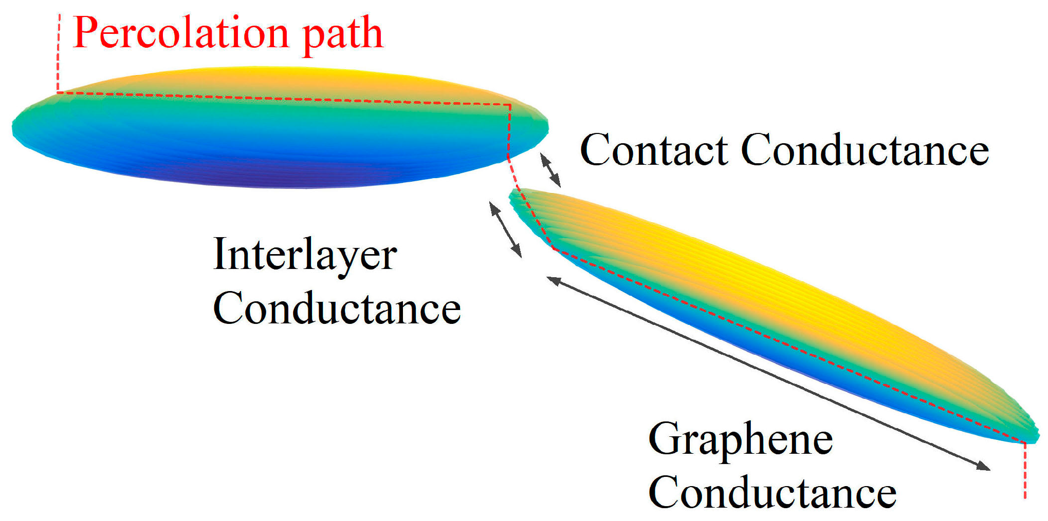
2.2. Graphene Conductance, Contact Conductance and Interlayer Conductance

Figure 2 shows a part of a percolation path. It can be seen that the conductance of the percolation path is composed of three parts in series: G_graphene, G_contact, and G_interlayer; G_graphene is the conductance of graphene and can be expressed by:

$$G_{graphene}=\frac{2e^2{N}_{chan}}{h},$$

(4)

where 2e²/h denotes the quantized conductance and N_chan is the number of channels for graphene that is proportional to the size of graphene N_chan = aD, where a is constant and we took a = 0.01 nm⁻¹ [33]. For D = 1 μm, one can get a sheet resistance 1/G_graphene = 1295 Ω/□, which is reasonable [34,35]. Here, electronic scattering behavior was ignored because D in our calculation was far less than the mean free path, which could exceed 28 μm [2].

The tunneling effects between GNPs were considered here. Once the distance between GNPs is within a few nanometers, tunneling can occur. Because the tunneling current exponentially increases with the decreasing distance, electron tunneling mainly occurs between the nearest two graphenes, which come from two different GNPs. Venugopal et al. [36] pointed out that only one or two layers of a graphene stack take the role of conducting current. The GNPs only interact with the first few layers, so we could calculate the contact conductance between the nearest two graphenes instead of that between GNPs. The tunneling effect could only be ignored if the distance between two GNPs exceeds the cut-off distance of 1.4 nm [37,38]. The contact conductance is the tunneling conductance between a pair of GNPs, and can be expressed as:

$$G_{contact}=G_{graphene}exp\left[-\frac{\sqrt{8m_e\Delta E}max\left(d_{GNPs},d_{vdW}\right)}{\hslash }\right],$$

(5)

where ΔE is the barrier height and d_GNPs is the distance between two GNPs. According to definition of the GNP in Equation (1), d_GNPs is equal to the distance between the two round faces minus the thickness of the GNP. The van der Waals separation distance d_vdW is the minimum distance between GNPs [39].

Thus the contact conductance between GNPs is tunneling conductance. The types of contacts between GNPs are point-to-point and point-to-face contact, so the computation of contact conductance based on quantum conductance is similar to the tunneling conductance between CNTs because of the small contact area. G_interlayer is the conductance between the top and bottom layer of a GNP, and the type of contacts between the graphene layers is face-to-face contact. Because of the large contact area, G_interlayer is much larger than G_contact and cannot be calculated by Equation (5). Here, we analyzed G_interlayer by the law of resistance. G_interlayer varies inversely with thickness [40] and can be expressed as:

$$G_{interlayer}=\frac{{\sigma }_3\pi D^2}{4l},$$

(6)

where σ₃ is the conductivity in the vertical direction of the GNP.

According to Equation (5), it can be estimated that G_contact is rather smaller than the conductance of the monolayer graphene G_graphene on account of d_vdW (between 0.3 and 0.4 nm [37,41,42]) and ΔE (several eV [43]). According to Equation (6), G_interlayer/G_graphene = σ₃πD²/4σ₁ld_vdW. Because σ₃ = 0.001σ₁ [22] or 0.1σ₁ [18], D > l, and D is generally on the micron level, which is about four orders of magnitude larger than d_vdW. We think that in general, G_graphene < G_interlayer. In this way, the relationship between the three conductivities can be obtained as follows: G_contact ≪ G_graphene < G_interlayer. Thus, each GNP is approximately equipotential.

2.3. Potential Equations of GNPs

Based on equipotential approximation, the potential equations of GNP can be constructed. For simplicity, we used U¹, U², and U³ to represent the potential of the GNP, the coated surface (CS), and the electrode, respectively. U¹ and U² are both an N × 1 matrix, and U³ is a 2 × 1 matrix. In order to compute the current flowing into the polymer, the CS is introduced, as shown in Figure 3. The CS is considered as the surface of f defined in Equation (1), taking ρ = l/2 + d, where d is the distance between the GNP and the corresponding CS. Next, we built the equations for U¹ and U².

For the ith GNP, based on the law of Kirchhoff, we have:

$${\displaystyle \sum }_{j=1}^N{G}_{ij}^{11}\left(U_i^1-U_j^1\right)+{\displaystyle \sum }_{j=1}^N{G}_{ij}^{12}\left(U_i^1-U_j^2\right)+{\displaystyle \sum }_{j=1}^2{G}_{ij}^{13}\left(U_i^1-U_j^3\right)=0,i=1,2,\dots ,N$$

(7)

The sum of these three currents is zero: the tunneling current between GNPs, the direct current from the GNPs to the CS, and the tunneling current from the GNPs to the electrodes. In this expression, G¹¹ is an N × N matrix of contact conductance, the elements of which can be evaluated as:

$$G_{ij}^{11}=\{\begin{array}{c}0,i=j\\ G_0{N}_{chan}exp\left[-\frac{\sqrt{8m_e\Delta E}max\left(d_{ij}^{11},d_{vdW}\right)}{\hslash }\right],i\ne j\end{array},$$

(8)

where $d_{ij}^{11}$ is the distance between GNPs, with:

$$d_{ij}^{11}=d_{ij}^g-l,$$

(9)

where $d_{ij}^g$ is the distance between the round face g_i and g_j. When the thickness l changes, one does not need to calculate $d_{ij}^g$ repeatedly to get $d_{ij}^{11}$. G¹² is also an N × N matrix, the elements of which are $G_{ij}^{12}$, the direct conductance between the ith GNP and the jth CS:

$$G_{ij}^{12}=\{\begin{array}{c}{\sigma }_{0}S/d,i=j\\ 0,i\ne j\end{array},$$

(10)

where S is the surface area of the GNP, S = πD²/2 + π²Dl/2 + πl², and σ₀ denotes the conductivity of the polymer. Trying to avoid the case in which the CS intersects with the GNPs, d needs to be small enough, so we took d = d_vdW/2 here. An N × 2 matrix G¹³ denotes the contact conductance between GNPs and electrodes, in consideration of van der Waals interactions, and $G_{ij}^{13}$ can be written as:

$$G_{ij}^{13}=G_0{N}_{chan}exp\left[-\frac{\sqrt{8m_e\Delta E}max\left(d_{ij}^{13},d_{vdW}\right)}{\hslash }\right],$$

(11)

where $d_{ij}^{13}$ denotes the distance between the GNPs and the electrodes.

In this way, Equation (7) can be evolved in linear equations as:

$$U^1=Q^{11}{U}^1+Q^{12}{U}^2+Q^{13}{U}^3,$$

(12)

where the elements of the matrix Q¹¹, Q¹², and Q¹³ are:

$$\begin{gathered} Q_{ij}^{11}=\frac{G_{ij}^{11}}{{{\displaystyle \sum }}_{j=1}^N\left(G_{ij}^{11}+G_{ij}^{12}\right)+{{\displaystyle \sum }}_{j=1}^2{G}_{ij}^{13}}, \\ {Q}_{ij}^{12}=\frac{G_{ij}^{12}}{{{\displaystyle \sum }}_{j=1}^N\left(G_{ij}^{11}+G_{ij}^{12}\right)+{{\displaystyle \sum }}_{j=1}^2{G}_{ij}^{13}}, \\ {Q}_{ij}^{13}=\frac{G_{ij}^{13}}{{{\displaystyle \sum }}_{j=1}^N\left(G_{ij}^{11}+G_{ij}^{12}\right)+{{\displaystyle \sum }}_{j=1}^2{G}_{ij}^{13}} \end{gathered}$$

(13)

2.4. Potential Equations of CS

Assuming that the matrix is an isotropic medium with uniform conductivity and permittivity, the electrical potential in matrix is determined by the Poisson equation:

$$\begin{array}{c}{\nabla }^{2}u\left(r\right)=-\frac{\rho }{\epsilon },r\in \Gamma \\ u\left(r\right)=U\left(r\right),r\in \partial \Gamma \end{array}.$$

(14)

where Γ and ∂Γ denote the matrix domain and its boundary, respectively. ρ is the volume charge density, and ε is the dielectric constant of polymer. Carriers injected from the electrodes are captured by the traps formed by the defects, interfaces, and impurities in the polymer medium, all of which turn out to be the volume charge. Our model calculates the conductivity of the composite under a constant electric field, so the volume charge in shallow traps migrates to the surface of the material under steady voltage, while the volume charge in deep traps is immovable and mainly concentrated near the electrode. On the one hand, the volume charge of non-uniform distribution makes it difficult to solve the Poisson equation; on the other hand, the space charge may vary the electric field distribution and carrier mobility, thus leading to a change in conductivity of the polymer. Therefore, in order to simplify the calculation, Equation (14) can be simplified to Laplace equation, and the effect of the volume charge on the calculation results could be reflected by setting a different conductivity of the polymer:

$$\begin{array}{c}{\nabla }^{2}u\left(r\right)=0,r\in \Gamma \\ u\left(r\right)=U\left(r\right),r\in \partial \Gamma \end{array}.$$

(15)

with:

$$U\left(r\right)=\{\begin{array}{c}{U}_i^1,r\in GN{P}_i,i=1,2,\dots ,N,\\ U_j^3,r\in E_j,j=1,2.\end{array}$$

(16)

where GNP_i is f_i (defined by Equation (1)) and E₁ and E₂ denote two electrodes. In particular, if r is in the overlapping domain, then U(r) is the average potential of coincident GNPs.

The solutions to Equation (15) can be obtained by WoS Monte Carlo simulations. Figure 4 shows an example, where r is the point where the potential is required in matrix. First, one draws a ball with r as its center. The ball needs to be big enough but cannot intersect any boundary ∂Γ. Next, a random point r⁽¹⁾ is generated on the surface of the ball. Then this step is repeated, and a trace is indicated with the red arrow. When the obtained r is close enough to a GNP or electrode, this random walk is stopped.

According to law of large numbers:

$$u\left(r\right)=\underset{M\to \infty }{lim}\frac{1}{M}{\displaystyle \sum }_{k=1}^{M}U\left(\partial {\Gamma }_k\right),$$

(17)

where $\partial {\Gamma }_k$ is the boundary that is closest to the terminal point and k is the ordinal number of random walk [44,45]. The potential at r is the expected value of the potential at the end of random walks. Equation (17) can be simplified to:

$$u\left(r\right)=\underset{M\to \infty }{lim}\frac{1}{M}{\displaystyle \sum }_{k=1}^M\left[{\displaystyle \sum }_{j=1}^N{U}_j^{1}P\left\{GN{P}_j|r\right\}+{\displaystyle \sum }_{j=1}^2{U}_j^{3}P\left\{E_j|r\right\}\right],$$

(18)

where P{GNP_j|r} and P{E_j|r} are Boolean variables that denote the events reaching GNP_j and E_j, respectively.

When putting r on a CS, Equation (18) can be expressed by:

$$U^2=Q^{21}{U}^1+Q^{23}{U}^3,$$

(19)

where the elements of the matrix Q²¹ and Q²³ are:

$$\begin{gathered} Q_{ij}^{21}=\underset{M\to \infty }{lim}\frac{1}{M}{\displaystyle \sum }_{k=1}^{M}P\left\{GN{P}_j|C{S}_i\right\}, \\ {Q}_{ij}^{23}=\underset{M\to \infty }{lim}\frac{1}{M}{\displaystyle \sum }_{k=1}^{M}P\left\{E_j|C{S}_i\right\}. \end{gathered}$$

(20)

For the detailed process of the WoS method to calculate Q²¹ and Q²³, refer to [32].

2.5. The Conductance of the Nanocomposite

Equations (12) and (19) are combined to get:

$$U=QU$$

(21)

where:

$$U=\left[\begin{array}{c}{U}^1\\ U^2\\ U^3\end{array}\right],Q=\left[\begin{array}{ccc}{Q}^{11}& Q^{12}& Q^{13}\\ Q^{21}& Q^{22}& Q^{23}\\ Q^{31}& Q^{32}& Q^{33}\end{array}\right].$$

(22)

where Q²² is the N × N zero matrix, Q³¹ and Q³² are both 2 × N zero matrixes, and Q³³ is a 2 × 2 unit matrix. The linear Equation (21) can be solved through an iterative approach.

We constructed a plane, z = d = d_vdW/2, that is parallel to the electrode, and the current of the composite material is equal to the current flowing through the plane, which can be calculated as:

$$I=\frac{L_x{L}_y{\sigma }_0\left(U_{z=d}-U_1^3\right)}{d}+{\displaystyle \sum }_{i=1}^N{G}_{i1}^{13}\left(U_i^1-U_1^3\right),$$

(23)

where U_{z = d} can be computed by the WoS method. The total current is the sum of the direct current from the plane to electrode 1 and the tunneling current from the GNPs to electrode 1. Moreover, the conductivity of the composite can be given as:

$$\sigma =\frac{I{L}_z}{\left(U_2^3-U_1^3\right)L_x{L}_y}.$$

(24)

3. Results and Discussion

Only four adjustable parameters are used in the whole calculation process: polymer conductivity σ₀, barrier height ΔE, thickness l, and the diameter D of the GNP. Figure 5 shows the volume fraction dependence of the conductivity of the GNP composite with various parameters. It can be seen that four sets of theoretical results fit well with the experimental data [18,19,46,47]. When the volume fraction was zero, the conductivity of the GNP composite was equal to that of the polymer; when the volume fraction increased, the conductivity increased slowly, because the filler was approximately equipotential and its role was to shorten the distance between two electrodes filled with the polymer. When no percolation path was formed in the material, there were two cases: (1) There were GNPs close to electrode 1 (less than cut off distance), where the potential of the GNPs was basically the same as that of electrode 1 because these GNPs did not form a percolation path; (2) there was no GNP close to electrode 1, so $G_{i1}^{13}$ was very small or even less than the conductivity of the polymer. In both cases, according to Equation (23), the tunneling current was almost zero, so the total current and the conductivity of the GNP composite were determined by direct current. When no percolation path was formed, with the GNP concentration increasing, the increase of U_{z = d} resulted in the increase of the total current, which caused the increase of conductivity by about one order of magnitude. This phenomenon was similar to that of the CNT composite, and the difference was that the conductivity of the CNT composite increased by about two or three orders of magnitude at this stage [32]. It can be seen that due to the differences in the shapes of the GNP and the CNT, the contribution of the GNP to conductivity was weaker than that of the CNT before the formation of the percolation path. When the concentration of the GNP was above the percolation threshold, a conductive network was formed between the two electrodes, and the potential of the GNP, which was close to electrode 1 (less than cut off distance), suddenly increased, resulting in a large tunneling current. Because the contact conductance between GNPs on a percolation path is greater than the direct conductance between GNPs, the tunneling current was much greater than the direct current, which resulted in a sharp rise in the conductivity. The tunneling current was related to the conductive network density and the number of GNPs on one path. With the further addition of GNPs, the number of percolation paths increased, and there may have been a shorter percolation path that brought about a further increase of the tunneling current and the conductivity. Similarly, above the percolation threshold, the increment of the conductivity of the GNP composite was smaller than that of the CNT composite [32], which might be attributable to the geometric properties of GNPs and CNTs.

Due to the influence of barrier height on contact conductance, we calculated the full range of conductivity of the GNP composite with various barrier heights, as shown in Figure 6. We found that the barrier height affected the conductivity above the percolation threshold, but it made no difference to the conductivity below the percolation threshold. This was because there was a non-zero tunneling current only when the percolation path was formed in the composite, which was affected by the barrier height. There was a tunneling effect between a close pair of GNPs. According to Equation (5), tunneling conductance is related to the width and height of a barrier. Barrier height is the difference between the work function of a GNP and the medium between GNPs, which may be a polymer or an interphase formed by molecular interaction between the GNP and the polymer. The tunneling effect makes the contact conductance exponentially decrease with the increase of barrier height. It is clear that the conductivity of a composite is determined by contact conductance after the percolation threshold. In addition, barrier height does not change the percolation threshold of GNP composites, but for CNT composites, the percolation threshold slightly increases with increases of barrier height [32]. The reason for this phenomenon is that the gap between fillers in a CNT network has a certain randomness. As barrier height increases, a part of the contact conductance between CNTs with a larger distance decreases sharply, which causes a percolation path break. Therefore, with an increase of barrier height, the number of percolation paths decreases or even disappears, leading to a slight rise in the percolation threshold of CNT composites. In a GNP network, most of the neighboring GNPs forming percolation paths overlap with each other. In this way, almost all the effective distance between overlapped GNPs takes the minimum value d_vdW. With the increase of barrier height, no percolation path fracture occurs. Therefore, barrier height does not affect the percolation threshold of a GNP composite.

The influence of polymer conductivity on the conductivity of GNP composites is illustrated in Figure 7. We took σ₀ = 10⁻¹⁵–10⁻⁹ S/m. It could be seen that the matrix conductivity only changed the part of conductivity below the percolation threshold. For instance, D = 1000 nm, l = 10 nm, ΔE = 3 eV, $d_{i1}^{13}$ = d_vdW, and σ₀ = 10⁻⁹ S/m; on the basis of Equation (11), $G_{i1}^{13}$ = 1.74 × 10⁻⁶ S. The direct conductance was L_xL_yσ₀/d = 5.8 × 10⁻¹⁰ S for L_x = L_y = 10 μm, which was much less than contact conductance. As a result, once the conductive network was established, the current of the GNP composites was determined by the tunneling current, and the conductivity was determined by contact conductance. The percolation threshold was closely associated with the formation of the conductive network in the composite without being influenced by the conductivity of the polymer.

In order to analyze the impact of aspect ratio of the filler GNP on the percolation threshold, the conductivities of composites with different thicknesses of GNPs were calculated, as shown in Figure 8a–c. Thickness changed in the range of 0.344–256 nm. The results suggested that the percolation threshold increased as l increased. If l < D, the number of GNPs needed to form percolation paths did not change with l, so when l was very small, the lower concentration of GNPs could form percolation paths. With l increasing, the concentration required to form percolation paths increased correspondingly. As the volume fraction of GNPs increased, more percolation path formation made the conductivity of the composite increase. Because of the randomness of the Monte Carlo method, the conductivity curve of the composite with the GNP volume fraction was not smooth.

Figure 6, Figure 7 and Figure 8 point out that the percolation threshold was greatly affected by the thickness of GNPs, but it had little relation to the barrier height and the conductivity of the polymer, so we calculated the percolation threshold with various aspect ratios of GNPs, as shown in Figure 9. The dotted line represents the theoretical results obtained from the base on the effective medium theory [24] and the exclusion volume [27]. The solid line is from our theoretical calculation. Various symbols are experimental data [18,19,46,48,49,50,51,52,53,54,55]. It can be seen that the result of Monte Carlo calculation was almost the same as that based on the effective medium theory. If the aspect ratio α < 0.1, then the curve could be approximately regarded as a straight line with a slope of 1, with a percolation threshold of Φ_C = 1.8α. Most pairs of GNPs with less than the cut off distance coincided in space if l was far less than D, so reducing l did not affect the formation of the percolation path. The simulation results showed good agreement with most of the experimental data, while a small part of the experimental data was larger than the theoretical data when α was small, which may have been caused by the aggregation of the synthesized GNPs in the polymer. If the aggregation of the inclusion occurred, the original percolation path was broken, which caused the percolation threshold to increase.

4. Concluding Remarks

In this paper, a Monte Carlo model was developed to calculate the conductivity of GNP composites. In this model, a GNP is considered to be a point set with a distance from random round faces less than half of the thickness of a GNP. Considering the electron tunneling effect, there was non-zero contact conductance between a pair of GNPs that were close to each other, which played a vital role for the conductivity of the composites. A set of linear equations about the potential of GNPs and CSs were established, where the potential of the CS was calculated by the WoS method. Then, the potential of each GNP was calculated. The conductivity of composites can be obtained by calculating the current through the plane z = d. There are only four adjustable parameters in the model: polymer conductivity σ₀, barrier height ΔE, thickness l, and the diameter D of GNPs. The conductivity of composites depends on the conductivity of a polymer σ₀ or barrier height ΔE, respectively, below or above the percolation threshold, and the percolation threshold is basically determined by the aspect ratio. The relationship between the conductivity and the volume fraction calculated by our theory agrees with the experimental data for four groups under corresponding parameters. The percolation threshold versus aspect ratio curve calculated by our theory was almost consistent with the analytical expression basis of the effective medium theory.

References

1. Mogera, U.; Kulkarni, G.U. A new twist in graphene research: Twisted graphene. Carbon 2020, 156, 470–487. [Google Scholar] [CrossRef]
2. Banszerus, L.; Schmitz, M.; Engels, S.; Goldsche, M.; Watanabe, K.; Taniguchi, T.; Beschoten, B. Ballistic transport exceeding 28μm in CVD grown graphene. Nano Lett. 2016, 16, 1387–1391. [Google Scholar] [CrossRef] [PubMed] [Green Version]
3. Dasgupta, A.; Rajukumar, L.P.; Rotella, C.; Lei, Y.; Terrones, M. Covalent three-dimensional networks of graphene and carbon nanotubes: Synthesis and environmental applications. Nano Today 2017, 12, 116–135. [Google Scholar] [CrossRef]
4. Gao, A.L.; Zhao, F.W.; Wang, F.; Zhang, G.F.; Zhao, S.; Cui, J.; Yan, Y.H. Highly conductive and light-weight acrylonitrile-butadiene-styrene copolymer/reduced graphene nanocomposites with segregated conductive structure. Compos. Part A Appl. Sci. Manuf. 2019, 112, 1–7. [Google Scholar] [CrossRef]
5. Oh, H.; Kim, K.; Ryu, S.; Kim, J. Enhancement of thermal conductivity of polymethyl methacrylate-coated graphene/epoxy composites using admicellar polymerization with different ionic surfactants. Compos. Part A Appl. Sci. Manuf. 2019, 116, 206–215. [Google Scholar] [CrossRef]
6. Hong, X.S.; Zheng, Y.Y.; Zhang, X.; Wu, X.Q. Preparation of graphene intercalated magnesium silicate for enhancing the thermal stability and thermal conductivity of ethylene-vinyl acetate copolymer. Polymer 2020, 193, 122332. [Google Scholar] [CrossRef]
7. Peng, W.X.; Sun, K. Effects of Cu/graphene interface on the mechanical properties of multilayer Cu/graphene composites. Mech. Mater. 2020, 141, 103270. [Google Scholar] [CrossRef]
8. Schueren, B.V.D.; Marouazi, H.E.; Mohanty, A.; Lévêque, P.; Sutter, C.; Romero, T.; Janowska, I. Polyvinyl alcohol-few layer graphene composite films prepared from aqueous colloids. Investigations of mechanical, conductive and gas barrier properties. Nanomaterials 2020, 10, 858. [Google Scholar] [CrossRef]
9. Li, P.C.; Zhu, B.H.; Li, P.; Zhang, Z.H.; Li, L.Y.; Gu, Y.Z. A facile method to synthesize CdSe-reduced graphene oxide composite with good dispersion and high nonlinear optical properties. Nanomaterials 2019, 9, 957. [Google Scholar] [CrossRef] [Green Version]
10. Liu, G.S.; Dai, S.X.; Zhu, B.H.; Li, P.; Wu, Z.K.; Gu, Y.Z. Third-order nonlinear optical properties of MoSe2/graphene composite materials. Opt. Laser Technol. 2019, 120, 105746. [Google Scholar] [CrossRef]
11. Pepłowski, A.; Walter, P.A.; Janczak, D.; Górecka, Z.; Swieszkowski, W.; Jakubowska, M. Solventless conducting paste based on graphene nanoplatelets for printing of flexible, standalone routes in room temperature. Nanomaterials 2018, 8, 829. [Google Scholar] [CrossRef] [PubMed] [Green Version]
12. Wang, B.; Ruan, T.T.; Chen, Y.; Jin, F.; Peng, L.; Zhou, Y.; Wang, D.L.; Dou, S.X. Graphene-based composites for electrochemical energy storage. Energy Storage Mater. 2020, 24, 22–51. [Google Scholar] [CrossRef]
13. Zhang, Z.Z.; Zhang, J.X.; Li, S.Y.; Liu, J.P.; Guo, Z.H. Effect of graphene liquid crystal on dielectric properties of polydimethylsiloxane nanocomposites. Compos. Part B Eng. 2019, 1761, 107338. [Google Scholar] [CrossRef]
14. Wang, L.; Wu, Y.; Wang, Y.; Li, H.F.; Jiang, N.S.; Niu, K.M. Laterally compressed graphene foam/acrylonitrile butadiene styrene composites for electromagnetic interference shielding. Compos. Part A Appl. Sci. Manuf. 2020, 133, 105887. [Google Scholar] [CrossRef]
15. Solis, C.G.; Enriquez, A.I.M.; Oliva, A.I.; Torre, A.R.L.; Oliva, J. Bioactivity of flexible graphene composites coated with a CaSiO3/acrylic polymer membrane. Mater. Chem. Phys. 2020, 2411, 122358. [Google Scholar] [CrossRef]
16. Zhao, B.W.; Sun, T.; Zhou, X.; Liu, X.Z.; Li, X.X.; Zhou, K.; Dong, L.H.; Wei, D.P. Three-dimensional graphene composite containing graphene-SiO2 nanoballs and its potential application in stress sensors. Nanomaterials 2019, 9, 438. [Google Scholar] [CrossRef] [Green Version]
17. Wang, F.; Zhao, D.S.; Zhang, L.B.; Fan, L.M.; Zhang, X.T.; Hu, S.N. Nanostructured nickel nitride with reduced graphene oxide composite bifunctional electrocatalysts for an efficient water-urea splitting. Nanomaterials 2019, 9, 1583. [Google Scholar] [CrossRef] [Green Version]
18. Stankovich, S.; Dikin, D.A.; Dommett, G.H.B.; Kohlhaas, K.M.; Zimney, E.J.; Stach, E.A.; Piner, R.D.; Nguyen, S.T.; Ruoff, R.S. Graphene-based composite materials. Nature 2006, 442, 282–286. [Google Scholar] [CrossRef]
19. Nistal, A.; Garcia, E.; Perez-Coll, D.; Prieto, C.; Belmonte, M.; Osendi, M.I.; Miranzo, P. Low percolation threshold in highly conducting graphene nanoplatelets/glass composite coatings. Carbon 2018, 139, 556–563. [Google Scholar] [CrossRef]
20. Bruggeman, D.A.G. Effective medium approximation for nonlinear conductivity of a composite medium. Ann. Phys. 1935, 24, 636–679. [Google Scholar] [CrossRef]
21. Weng, G.J. A dynamical theory for the Mori–Tanaka and Ponte Castañeda–Willis estimates. Mech. Mater. 2010, 42, 886–893. [Google Scholar] [CrossRef]
22. Xia, X.D.; Wang, Y.; Zhong, Z.; Weng, G.J. A theory of electrical conductivity, dielectric constant, and electromagnetic interference shielding for lightweight graphene composite foams. J. Appl. Phys. 2016, 120, 085102. [Google Scholar] [CrossRef]
23. Xia, X.D.; Hao, J.; Wang, Y.; Zhong, Z.; Weng, G.J. Theory of electrical conductivity and dielectric permittivity of highly aligned graphene-based nanocomposites. J. Phys. Condens. Matter. 2017, 29, 205702. [Google Scholar] [CrossRef] [PubMed]
24. Wang, Y.; Shan, J.W.; Weng, G.J. Percolation threshold and electrical conductivity of graphene-based nanocomposites with filler agglomeration and interfacial tunneling. J. Appl. Phys. 2015, 118, 065101. [Google Scholar] [CrossRef]
25. Hashemi, R.; Weng, G.J. A theoretical treatment of graphene nanocomposites with percolation threshold, tunneling-assisted conductivity and microcapacitor effect in AC and DC electrical settings. Carbon 2016, 96, 474–490. [Google Scholar] [CrossRef]
26. Xia, X.D.; Wang, Y.; Zhong, Z.; Weng, G.J. A frequency-dependent theory of electrical conductivity and dielectric permittivity for graphene-polymer nanocomposites. Carbon 2017, 111, 221–230. [Google Scholar] [CrossRef]
27. Torquato, S.; Jiao, Y. Effect of dimensionality on the percolation threshold of overlapping nonspherical hyperparticles. Phys. Rev. E 2013, 87, 022111. [Google Scholar] [CrossRef] [Green Version]
28. Mathew, M.; Schilling, T.; Oettel, M. Connectivity percolation in suspensions of hard platelets. Phys. Rev. E 2012, 85, 061407. [Google Scholar] [CrossRef] [Green Version]
29. Oskouyi, A.B.; Mertiny, P. Monte Carlo model for the study of percolation thresholds in composites filled with circular conductive nano-disks. Procedia Eng. 2011, 10, 403–408. [Google Scholar] [CrossRef] [Green Version]
30. Wang, W.L.; Jayatissa, A.H. Computational and experimental study of electrical conductivity of graphene/poly(methyl methacrylate) nanocomposite using Monte Carlo method and percolation theory. Synthetic Met. 2015, 204, 141–147. [Google Scholar] [CrossRef]
31. Zabihi, Z.; Araghi, H. Monte Carlo simulations of effective electrical conductivity of graphene/poly(methyl methacrylate) nanocomposite: Landauer-Buttiker approach. Synthetic Met. 2016, 217, 87–93. [Google Scholar] [CrossRef]
32. Fang, C.; Zhang, J.J.; Chen, X.Q.; Weng, G.J. A Monte Carlo model with equipotential approximation and tunneling resistance for the electrical conductivity of carbon nanotube polymer composites. Carbon 2019, 146, 125–138. [Google Scholar] [CrossRef]
33. Naeemi, A.; Meindl, J.D. Compact Physical Models for Multiwall Carbon-Nanotube Interconnects. IEEE Electr. Device Lett. 2006, 27, 338–340. [Google Scholar] [CrossRef]
34. Peng, S.; Jin, Z.; Ma, P.; Zhang, D.Y.; Shi, J.Y.; Niu, J.B.; Wang, X.Y.; Wang, S.Q.; Li, M.; Liu, X.Y.; et al. The sheet resistance of graphene under contact and its effect on the derived specific contact resistivity. Carbon 2015, 82, 500–505. [Google Scholar] [CrossRef]
35. Smith, J.T.; Franklin, A.D.; Farmer, D.B.; Dimitrakopoulos, C.D. Reducing Contact Resistance in Graphene Devices through Contact Area Patterning. ACS Nano 2013, 7, 3661–3667. [Google Scholar] [CrossRef]
36. Venugopal, A.; Colombo, L.; Vogel, E.M. Contact resistance in few and multilayer graphene devices. Appl. Phys. Lett. 2010, 96, 013512. [Google Scholar] [CrossRef]
37. Bao, W.S.; Meguid, S.A.; Zhu, Z.H.; Weng, G.J. Tunneling resistance and its effect on the electrical conductivity of carbon nanotube nanocomposites. J. Appl. Phys. 2012, 111, 093726. [Google Scholar] [CrossRef]
38. Gong, S.; Zhu, Z.H.; Haddad, E.I. Modeling electrical conductivity of nanocomposites by considering carbon nanotube deformation at nanotube junctions. J. Appl. Phys. 2013, 114, 074303. [Google Scholar] [CrossRef]
39. Hertel, T.; Walkup, R.E.; Avouris, P. Deformation of carbon nanotubes by surface van der Waals forces. Phys. Rev. B 1998, 58, 13870–13873. [Google Scholar] [CrossRef]
40. Nirmalraj, P.N.; Lutz, T.; Kumar, S.; Duesberg, G.S.; Boland, J.J. Nanoscale Mapping of Electrical Resistivity and Connectivity in Graphene Strips and Networks. Nano Lett. 2011, 11, 16–22. [Google Scholar] [CrossRef]
41. Vivo, B.D.; Lamberti, P.; Spinelli, G.; Tucci, V.; Vertuccio, L.; Vittoria, V. Simulation and experimental characterization of polymer/carbon nanotubes composites for strain sensor applications. J. Appl. Phys. 2014, 116, 054307. [Google Scholar] [CrossRef]
42. Aitken, Z.H.; Huang, R. Effects of mismatch strain and substrate surface corrugation on morphology of supported monolayer graphene. J. Appl. Phys. 2010, 107, 123531. [Google Scholar] [CrossRef]
43. Peng, X.H.; Tang, F.; Copple, A. Engineering the work function of armchair graphene nanoribbons using strain and functional species: A first principles study. J Phys. Condens. Matter 2012, 24, 075501. [Google Scholar] [CrossRef] [PubMed] [Green Version]
44. Reynolds, J.F. A proof of the random-walk method for solving Laplace’s equation in 2-D. Math. Gaz. 1965, 49, 416–420. [Google Scholar] [CrossRef]
45. Kyprianou, A.E.; Osojnik, A.; Shardlow, T. Unbiased ‘walk-on-spheres’ Monte Carlo methods for the fractional Laplacian. IMA J. Numer. Anal. 2018, 38, 1550–1578. [Google Scholar] [CrossRef]
46. Zhang, H.B.; Zheng, W.G.; Yan, Q.; Yang, Y.; Wang, J.; Lu, Z.H.; Ji, G.Y.; Yu, Z.Z. Electrically conductive polyethylene terephthalate/graphene nanocomposites prepared by melt compounding. Polymer 2010, 51, 1191–1196. [Google Scholar] [CrossRef]
47. Kim, S.Y.; Noh, Y.J.; Yu, J. Prediction and experimental validation of electrical percolation by applying a modifified micromechanics model considering multiple heterogeneous inclusions. Compos. Sci. Technol. 2015, 106, 156–162. [Google Scholar] [CrossRef]
48. Ramirez, C.; Figueiredo, F.M.; Miranzo, P.; Poza, P.; Osendi, M.I. Graphene nanoplatelet/silicon nitride composites with high electrical conductivity. Carbon 2012, 50, 3607–3615. [Google Scholar] [CrossRef]
49. Tan, Y.Q.; Luo, H.; Zhang, H.B.; Peng, S.M. Graphene nanoplatelet reinforced boron carbide composites with high electrical and thermal conductivity. J. Eur. Ceram. Soc. 2016, 36, 2679–2687. [Google Scholar] [CrossRef]
50. Yue, L.; Pircheraghi, G.; Monemian, S.A.; Zloczower, I.M. Epoxy composites with carbon nanotubes and graphene nanoplatelets—Dispersion and synergy effects. Carbon 2014, 78, 268–278. [Google Scholar] [CrossRef]
51. Fan, Y.C.; Wang, L.J.; Li, J.L.; Li, J.Q.; Sun, S.K.; Chen, F.; Chen, L.D.; Jiang, W. Preparation and electrical properties of graphene nanosheet/Al2O3 composites. Carbon 2010, 48, 1743–1749. [Google Scholar] [CrossRef]
52. Pu, N.W.; Peng, Y.Y.; Wang, P.C.; Chen, C.Y.; Shi, J.N.; Liu, Y.M.; Ger, M.D.; Chang, C.L. Application of nitrogen-doped graphene nanosheets in electrically conductive adhesives. Carbon 2014, 67, 449–456. [Google Scholar] [CrossRef]
53. Zheng, W.; Chen, W.G.; Zhao, Q.; Ren, S.X.; Fu, Y.Q. Interfacial structures and mechanisms for strengthening and enhanced conductivity of graphene/epoxy nanocomposites. Polymer 2019, 163, 171–177. [Google Scholar] [CrossRef]
54. Simsek, I.N.G.; Nistal, A.; García, E.; Coll, D.P.; Miranzo, P.; Osendi, M.I. The effect of graphene nanoplatelets on the thermal and electrical properties of aluminum nitride ceramics. J. Eur. Ceram. Soc. 2017, 37, 3721–3729. [Google Scholar] [CrossRef]
55. Yun, C.; Feng, Y.B.; Qiu, T.; Yang, J.; Li, X.Y.; Yua, L. Mechanical, electrical, and thermal properties of graphene nanosheet/aluminum nitride composites. Ceram. Int. 2015, 41, 8643–8649. [Google Scholar] [CrossRef]
Figure 1. Schematics of (a) graphene nanoplatelet (GNP) network in a representative volume element (RVE) and (b) position and orientation of the GNP.
Nanomaterials 10 01129 g001
Figure 2. A diagram of Ggraphene (the conductance of graphene), Ginterlayer (the conductance between the top and bottom layer of a GNP), and Gcontact (the tunneling conductance between a pair of GNPs).
Nanomaterials 10 01129 g002
Figure 3. A coated surface (CS) on a GNP.
Nanomaterials 10 01129 g003
Figure 4. A random walk process on a sphere.
Nanomaterials 10 01129 g004
Figure 5. Numerical simulation results and experimental data of conductivity: (a) with Zhang et al. [46], (b) with Stankovich et al. [18], (c) with Kim et al. [47], and (d) with Nistal et al. [19].
Nanomaterials 10 01129 g005aNanomaterials 10 01129 g005b
Figure 6. Tunneling effects of different barrier heights on the conductivity of GNP composites.
Nanomaterials 10 01129 g006
Figure 7. Electrical conductivity of GNP composites of different polymer conductivities.
Nanomaterials 10 01129 g007
Figure 8. Electrical conductivity of GNP composites with different GNP thicknesses: (a) l = 0.344, 0.69, 1, and 2 nm; (b) l = 4, 8, 16, and 32 nm; and (c) l = 64, 128, 256, and 512 nm.
Nanomaterials 10 01129 g008aNanomaterials 10 01129 g008b
Figure 9. Percolation threshold versus aspect ratio.
Nanomaterials 10 01129 g009