Faster ≠ Smarter: Children with Higher Levels of Ability Take Longer to Give Incorrect Answers, Especially When the Task Matches Their Ability


Abstract
:1. Introduction
We hear school men very authoritatively saying that the fast students make the best grades and the slow ones the poorest. Statements of this kind are usually based on the assumption that if a student knows the subject in which he is being tested it should follow that he requires but a short time to make his answer. Needless to say, this assumption merits confirmation(Longstaff and Porter 1928, p. 638; as cited in Gernsbacher et al. 2020).
1.1. The Uncertain Role of Intelligence
1.2. Refuting the Stereotype
1.3. The F > C Phenomenon
1.4. The Distance–Difficulty Hypothesis
1.5. The Proposed Model
2. Materials and Methods
2.1. Participants
2.2. Measures
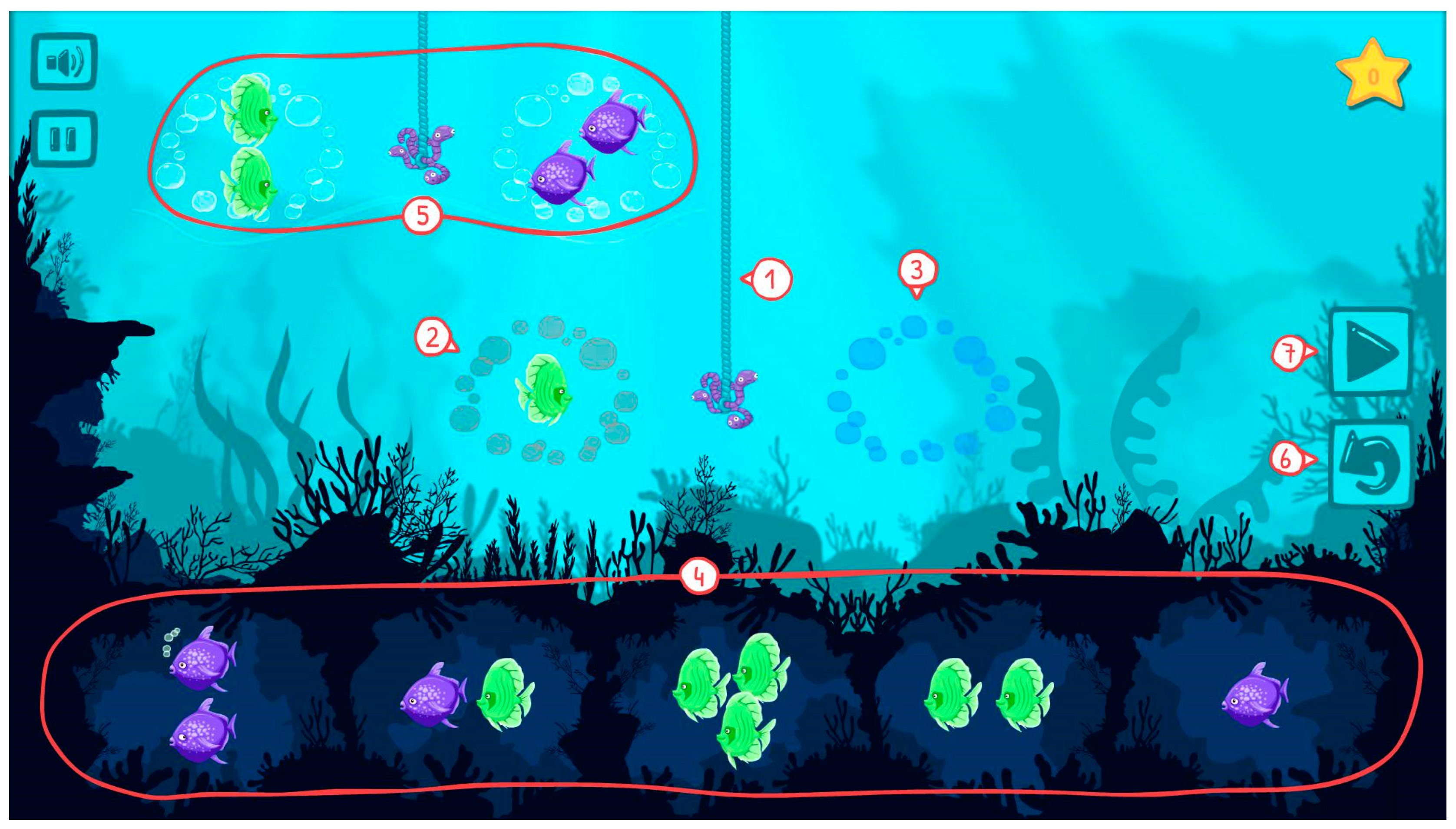
Triton and the Hungry Ocean
2.3. Data Management
2.4. Analysis plan
2.4.1. Preliminary IRT Models
2.4.2. Main Analyses
3. Results
3.1. Ability Estimates
3.2. Null Model
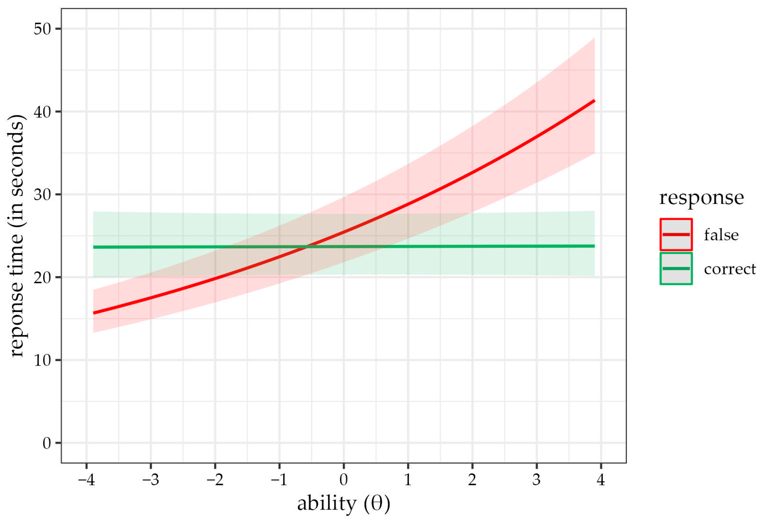
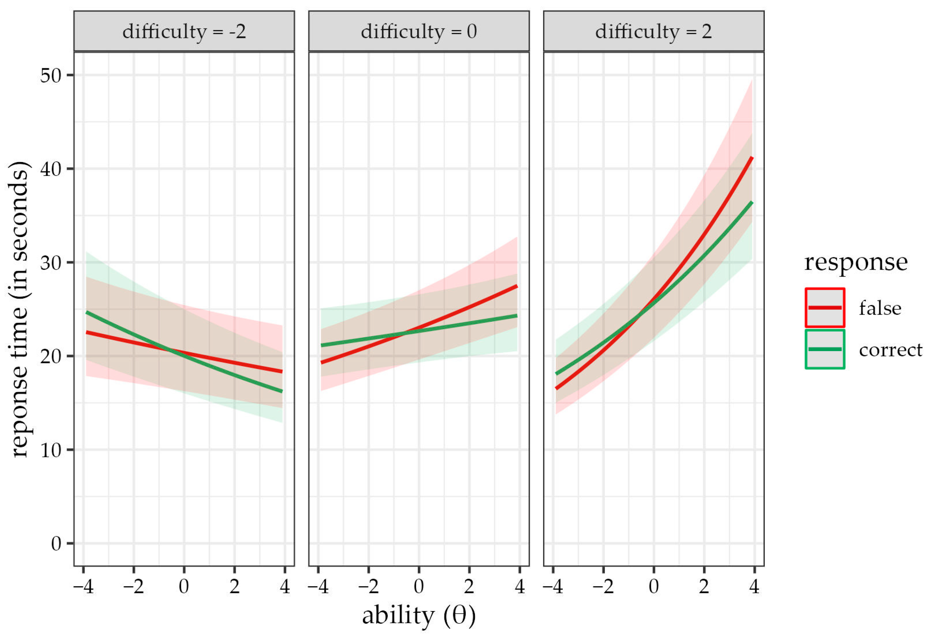
3.3. Models Assessing the F > C Phenomenon

| Model 0 | Model A1 | Model A2 | Model A3 | ||||||||||||||
|---|---|---|---|---|---|---|---|---|---|---|---|---|---|---|---|---|---|
| 95% CI | 95% CI | 95% CI | 95% CI | ||||||||||||||
| coef. | est. | LL | UL | est. | LL | UL | est. | LL | UL | est. | LL | UL | |||||
| Fixed effects | |||||||||||||||||
| intercept | μ | 3.16 | *** | 3.00 | 3.33 | 3.18 | *** | 3.02 | 3.35 | 3.15 | *** | 2.99 | 3.31 | 3.19 | *** | 3.03 | 3.36 |
| correct answer (FC) | γ1 | −0.04 | ** | −0.06 | −0.01 | −0.05 | *** | −0.08 | −0.03 | −0.07 | *** | −0.09 | −0.04 | ||||
| item difficulty | γ2 | 0.05 | 0.00 | 0.12 | 0.05 | 0.00 | 0.11 | ||||||||||
| person ability | γ3 | 0.06 | *** | 0.05 | 0.07 | 0.12 | *** | 0.11 | 0.14 | ||||||||
| FC × ability | γ13 | −0.12 | *** | −0.13 | −0.11 | ||||||||||||
| Random effects | |||||||||||||||||
| person intercept variance | var(τj) | 0.07 | *** | 0.06 | 0.08 | 0.07 | *** | 0.06 | 0.08 | 0.06 | *** | 0.05 | 0.07 | 0.06 | *** | 0.05 | 0.07 |
| item intercept variance | var(βi) | 0.20 | *** | 0.12 | 0.33 | 0.19 | *** | 0.11 | 0.32 | 0.17 | *** | 0.09 | 0.28 | 0.17 | *** | 0.10 | 0.29 |
| residual variance | var(εij) | 0.37 | *** | 0.36 | 0.38 | 0.37 | *** | 0.36 | 0.38 | 0.37 | *** | 0.36 | 0.38 | 0.36 | *** | 0.35 | 0.37 |
| Goodness of fit | |||||||||||||||||
| conditional R2 | 0.417 | 0.415 | 0.422 | 0.439 | |||||||||||||
| marginal R2 | 0.000 | 0.001 | 0.055 | 0.070 | |||||||||||||
| log-likelihood | −14,193 | −14,189 | −14,154 | −14,008 | |||||||||||||
| AIC | 28,395 | 28,389 | 28,323 | 28,031 | |||||||||||||
| BIC | 28,425 | 28,427 | 28,376 | 28,092 | |||||||||||||
| Δχ2 (df) | 8.09 (1) | ** | 70.08 (2) | *** | 293.23 (1) | *** | |||||||||||
| 95% CI | |||||
|---|---|---|---|---|---|
| coef. | est. | LL | UL | ||
| Fixed effects | |||||
| intercept | μ | 3.14 | *** | 2.98 | 3.30 |
| correct answer (FC) | γ1 | −0.02 | −0.04 | 0.01 | |
| item difficulty | γ2 | 0.06 | 0.00 | 0.12 | |
| person ability | γ3 | 0.05 | *** | 0.03 | 0.06 |
| FC × ability | γ13 | −0.03 | *** | −0.04 | −0.01 |
| difficulty × ability | γ23 | 0.04 | *** | 0.03 | 0.04 |
| Random effects | |||||
| person intercept variance | var(τj) | 0.06 | *** | 0.05 | 0.07 |
| item intercept variance | var(βi) | 0.17 | *** | 0.10 | 0.28 |
| residual variance | var(εij) | 0.34 | *** | 0.33 | 0.35 |
| Goodness of fit | |||||
| conditional R2 | 0.466 | ||||
| marginal R2 | 0.097 | ||||
| log-likelihood | −13,606 | ||||
| AIC | 27,231 | ||||
| BIC | 27,300 | ||||
| Δχ2 (df) | 802.28 (1) | *** | |||
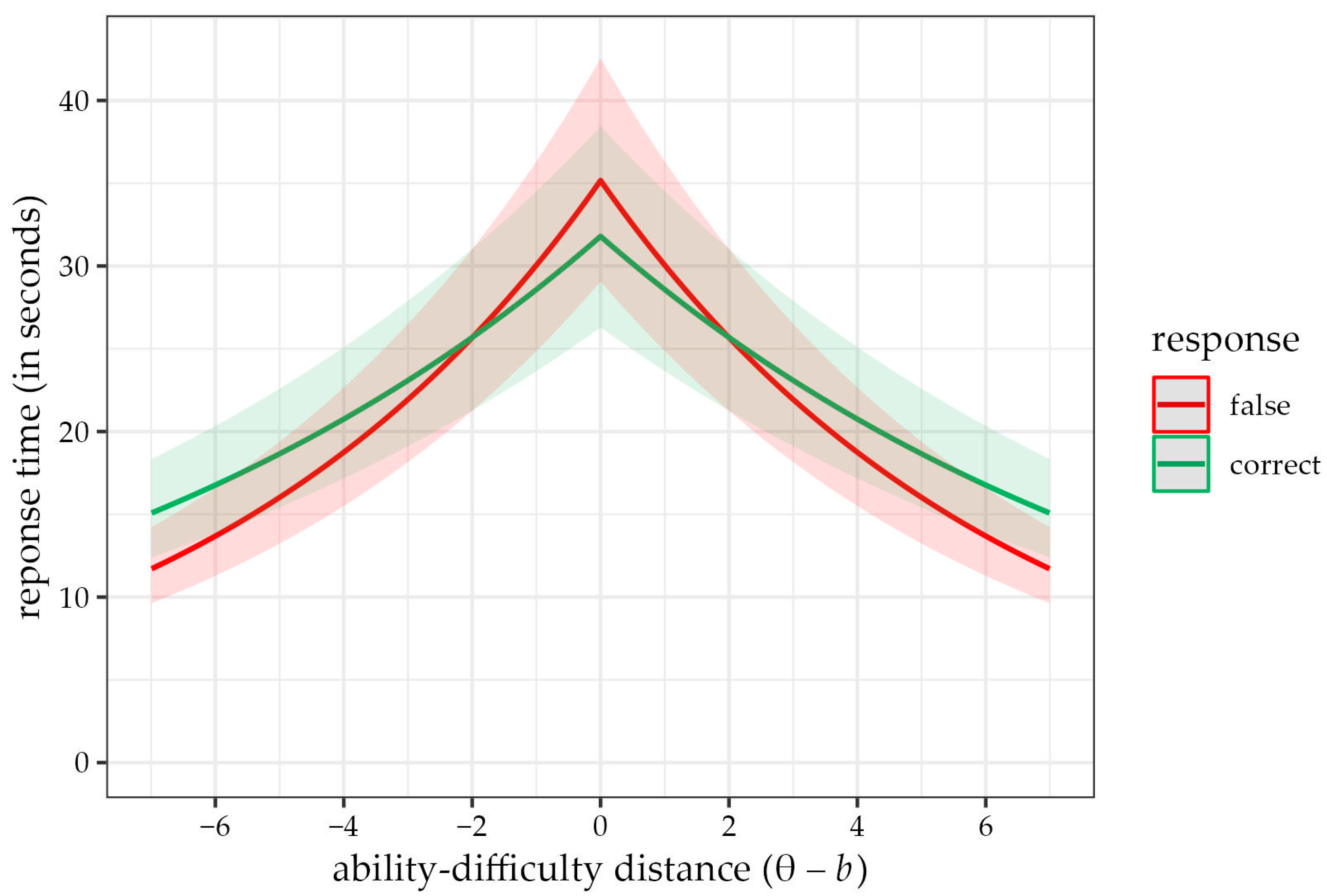
3.4. Models Assessing the Distance–Difficulty Hypothesis
4. Discussion
Supplementary Materials
Author Contributions
Funding
Institutional Review Board Statement
Informed Consent Statement
Data Availability Statement
Conflicts of Interest
Appendix A
Appendix B
| Response Correctness | Response Time (in Seconds) | |||||||
|---|---|---|---|---|---|---|---|---|
| Item | Sample | Guessing | Difficulty | M | SD | M | SD | Mdn |
| item 1 | 514 | 0.200 | −1.28 | 0.75 | 0.43 | 21.19 | 24.57 | 15.00 |
| item 2 | 514 | 0.200 | −1.91 | 0.81 | 0.39 | 19.52 | 17.80 | 14.50 |
| item 3 | 514 | 0.067 | −3.35 | 0.91 | 0.28 | 31.75 | 24.68 | 24.00 |
| item 4 | 514 | 0.067 | −3.12 | 0.90 | 0.30 | 20.80 | 21.49 | 16.50 |
| item 5 | 514 | 0.050 | −1.26 | 0.71 | 0.46 | 47.71 | 38.18 | 35.50 |
| item 6 | 514 | 0.067 | −2.32 | 0.83 | 0.37 | 20.07 | 15.59 | 15.50 |
| item 7 | 514 | 0.200 | −1.97 | 0.84 | 0.37 | 15.96 | 25.88 | 10.00 |
| item 8 | 514 | 0.100 | −2.54 | 0.86 | 0.35 | 24.81 | 21.55 | 18.00 |
| item 9 | 514 | 0.200 | 0.17 | 0.59 | 0.49 | 13.52 | 10.57 | 10.00 |
| item 10 | 514 | 0.050 | −1.62 | 0.76 | 0.43 | 34.38 | 19.46 | 28.50 |
| item 11 | 514 | 0.200 | −0.54 | 0.68 | 0.47 | 22.89 | 18.04 | 17.50 |
| item 12 | 514 | 0.200 | −1.55 | 0.79 | 0.41 | 10.87 | 8.86 | 8.50 |
| item 13 | 514 | 0.200 | 2.91 | 0.25 | 0.44 | 15.92 | 16.14 | 11.00 |
| item 14 | 514 | 0.050 | −0.17 | 0.56 | 0.50 | 51.22 | 30.05 | 44.20 |
| item 15 | 514 | 0.200 | 0.99 | 0.49 | 0.50 | 27.23 | 19.43 | 21.00 |
| item 16 | 514 | 0.017 | 0.31 | 0.46 | 0.50 | 50.40 | 33.98 | 42.50 |
| item 17 | 514 | 0.200 | 1.40 | 0.44 | 0.50 | 31.63 | 24.05 | 26.00 |
| item 18 | 514 | 0.200 | 1.29 | 0.42 | 0.49 | 25.93 | 20.69 | 20.00 |
| item 19 | 514 | 0.050 | 0.35 | 0.48 | 0.50 | 42.44 | 28.52 | 34.25 |
| item 20 | 514 | 0.200 | 1.74 | 0.38 | 0.49 | 42.19 | 32.50 | 33.75 |
| item 21 | 514 | 0.200 | 2.19 | 0.32 | 0.47 | 29.14 | 23.76 | 22.50 |
| item 22 | 514 | 0.067 | 3.15 | 0.19 | 0.39 | 61.93 | 53.74 | 45.75 |
| item 23 | 514 | 0.200 | 1.44 | 0.40 | 0.49 | 25.45 | 19.60 | 19.50 |
| item 24 | 510 | 0.100 | 3.60 | 0.16 | 0.37 | 43.21 | 36.16 | 31.75 |
| item 25 | 507 | 0.050 | 3.09 | 0.15 | 0.36 | 60.81 | 52.38 | 46.00 |
| item 26 | 504 | 0.200 | 4.88 | 0.15 | 0.36 | 39.15 | 42.53 | 26.50 |
| item 27 | 502 | 0.200 | 3.71 | 0.28 | 0.45 | 31.27 | 28.12 | 22.50 |
| item 28 | 500 | 0.050 | 5.23 | 0.06 | 0.24 | 44.33 | 37.55 | 33.50 |
| item 29 | 496 | 0.017 | 5.80 | 0.04 | 0.19 | 45.70 | 40.60 | 35.00 |
| 1 | In this study, we use the terms ‘item’ and ‘task’ semi-interchangeably. The word ‘item’ refers to a clearly demarcated part of the test whose psychometric difficulty can be empirically extracted. The word ‘task’ refers to the content of the item. In the case of Triton, children solve the same ‘task’ (balance both sides of the equation) many times, though are administered ‘items’ of varying difficulty. |
| 2 | Please note that the individual effects of item difficulty (bi) and a person’s ability (θj) are not included in the model, as they are already used to form the distance–difficulty difference term. |
References
- Baayen, R. Harald, Douglas J. Davidson, and Douglas M. Bates. 2008. Mixed-effects modeling with crossed random effects for subjects and items. Journal of Memory and Language 59: 390–412. [Google Scholar] [CrossRef]
- Bates, Douglas, Martin Mächler, Ben Bolker, and Steve Walker. 2015. Fitting Linear Mixed-Effects Models Using Lme4. Journal of Statistical Software 67: 1–48. [Google Scholar] [CrossRef]
- Beckmann, Jens F. 2000. Differentielle Latenzzeiteffekte Bei Der Bearbeitung von Reasoning-Items [Differential Effects on Latencies in Solving Reasoning Items]. Diagnostica 46: 124–29. [Google Scholar] [CrossRef]
- Beckmann, Jens F., and Nadin Beckmann. 2005. Effects of Feedback on Performance and Response Latencies in Untimed Reasoning Tests. Psychology Science 47: 262–78. [Google Scholar]
- Beckmann, Jens F., Jürgen Guthke, and Hans Vahle. 1997. Analysen Zum Zeitverhalten Bei Computergestützten Adaptiven Intelligenz-Lerntests. Diagnostica 43: 40–62. [Google Scholar]
- Bond, Trevor G., and Christine M. Fox. 2013. Applying the Rasch Model: Fundamental Measurement in the Human Sciences. London: Psychology Press. [Google Scholar]
- Borsboom, Denny, and Gideon J. Mellenbergh. 2004. Why Psychometrics Is Not Pathological: A Comment on Michell. Theory & Psychology 14: 105–20. [Google Scholar] [CrossRef]
- Bouffard-Bouchard, Thérèse, Sophie Parent, and Serge Lavirée. 1993. Self-regulation on a concept-formation task among average and gifted students. Journal of Experimental Child Psychology 56: 115–34. [Google Scholar] [CrossRef]
- Brighton, Catherine M. 2003. The Effects of Middle School Teachers’ Beliefs on Classroom Practices. Journal for the Education of the Gifted 27: 177–206. [Google Scholar] [CrossRef]
- Chalmers, R. Philip. 2012. Mirt: A Multidimensional Item Response Theory Package for TheREnvironment. Journal of Statistical Software 48: 1–29. [Google Scholar] [CrossRef]
- Cross, Dionne I. 2009. Alignment, Cohesion, and Change: Examining Mathematics Teachers’ Belief Structures and Their Influence on Instructional Practices. Journal of Mathematics Teacher Education 12: 325–46. [Google Scholar] [CrossRef]
- Cucina, Jeffrey M., Sharron T. Peyton, Chihwei Su, and Kevin A. Byle. 2016. Role of Mental Abilities and Mental Tests in Explaining High-School Grades. Intelligence 54: 90–104. [Google Scholar] [CrossRef]
- de Ayala, R. J., Bruno D. Zumbo, David J. Weiss, Mark Reckase, and Scott Hofer. 2022. The Theory and Practice of Item Response Theory the Theory and Practice of Item Response Theory. London: Guilford Press. [Google Scholar]
- De Boeck, Paul, and Mark Wilson, eds. 2004. Explanatory Item Response Models: A Generalised Linear and Nonlinear Approach. New York: Springer, vol. 10. [Google Scholar]
- Eun, Barohny. 2019. The Zone of Proximal Development as an Overarching Concept: A Framework for Synthesizing Vygotsky’s Theories. Educational Philosophy and Theory 51: 18–30. [Google Scholar] [CrossRef]
- Ferrando, Pere J., and Urbano Lorenzo-Seva. 2007. An Item Response Theory Model for Incorporating Response Time Data in Binary Personality Items. Applied Psychological Measurement 31: 525–43. [Google Scholar] [CrossRef]
- Gernsbacher, Morton Ann, Raechel N. Soicher, and Kathryn A. Becker-Blease. 2020. Four Empirically Based Reasons Not to Administer Time-Limited Tests. Translational Issues in Psychological Science 6: 175–90. [Google Scholar] [CrossRef] [PubMed]
- Goldhammer, Frank, Johannes Naumann, Annette Stelter, Krisztina Tóth, Heiko Rölke, and Eckhard Klieme. 2014. The time on task effect in reading and problem solving is moderated by task difficulty and skill: Insights from a computer-based large-scale assessment. Journal of Educational Psychology 106: 608. [Google Scholar] [CrossRef]
- Gravemeijer, Koeno. 2020. A Socio-Constructivist Elaboration of Realistic Mathematics Education. In National Reflections on the Netherlands Didactics of Mathematics. Cham: Springer, pp. 217–33. [Google Scholar]
- Howard, Steven James, and Elena Vasseleu. 2020. Self-regulation and executive function longitudinally predict advanced learning in preschool. Frontiers in Psychology 11: 49. [Google Scholar] [CrossRef]
- Inhelder, Bärbel, and Jean Piaget. 1958. The Growth of Logical Thinking from Childhood to Adolescence: An Essay on the Construction of Formal Operational Structures. London: Psychology Press, vol. 22. [Google Scholar]
- Jensen, Arthur R. 2011. The Theory of Intelligence and Its Measurement. Intelligence 39: 171–77. [Google Scholar] [CrossRef]
- Kan, Kees-Jan, Han L. J. van der Maas, and Stephen Z. Levine. 2019. Extending Psychometric Network Analysis: Empirical Evidence against g in Favor of Mutualism? Intelligence 73: 52–62. [Google Scholar] [CrossRef]
- Kumle, Levi, Melissa L.-H. Võ, and Dejan Draschkow. 2021. Estimating Power in (Generalized) Linear Mixed Models: An Open Introduction and Tutorial in R. Behavior Research Methods 53: 2528–43. [Google Scholar] [CrossRef]
- Linacre, John Michael. 2002. Dichotomous Quasi-Rasch Model with Guessing. Rasch Measurement Transactions 15: 856. [Google Scholar]
- McGrew, Kevin S., Erica M. LaForte, and Fredrick A. Schrank. 2014. Technical Manual: Woodcock-Johnson IV. Rolling Meadows: Riverside. [Google Scholar]
- Perry, Laura B. 2005. The Seeing and the Seen: Contrasting Perspectives of Post-communist Czech Schooling. Compare: A Journal of Comparative and International Education 35: 265–83. [Google Scholar] [CrossRef]
- Pfeiffer, Steven I., and Tania Jarosewich. 2003. GRS: Gifted Rating Scales. San Antonio: Psychological Corporation. [Google Scholar]
- Preckel, Franzis, and Philipp Alexander Freund. 2005. Accuracy, Latency, and Confidence in Abstract Reasoning: The Influence of Fear of Failure and Gender. Psychology Science 47: 230. [Google Scholar]
- R Core Team. 2021. R: A Language and Environment for Statistical Computing. Vienna: R Foundation for Statistical Computing. Available online: https://www.R-project.org/ (accessed on 22 March 2023).
- Renzulli, Joseph. 2021. Scales for Rating the Behavioral Characteristics of Superior Students: Technical and Administration Manual. London: Routledge. [Google Scholar]
- Roth, Wolff-Michael. 2020. Zone of Proximal Development in Mathematics Education. In Encyclopedia of Mathematics Education. Cham: Springer, pp. 913–16. [Google Scholar]
- Ryser, Gail R., and Kathleen McConnell. 2004. Scales for Identifying Gifted Students. Waco: Prufrock Press Inc. [Google Scholar]
- Savasci, Funda, and Donna F. Berlin. 2012. Science Teacher Beliefs and Classroom Practice Related to Constructivism in Different School Settings. Journal of Science Teacher Education 23: 65–86. [Google Scholar] [CrossRef]
- Scherer, Ronny, Samuel Greiff, and Jarkko Hautamäki. 2015. Exploring the relation between time on task and ability in complex problem solving. Intelligence 48: 37–50. [Google Scholar] [CrossRef]
- Schneider, W. Joel, and Kevin S. McGrew. 2018. The Cattell–Horn–Carroll Theory of Cognitive Abilities. In Contemporary Intellectual Assessment: Theories, Tests, and Issues, 4th ed. New York: The Guilford Press, pp. 73–163. [Google Scholar]
- Seeley, Cathy L. 2009. Faster Isn’t Smarter: Messages about Math, Teaching, and Learning in the 21st Century: A Resource for Teachers, Leaders, Policy Makers, and Families. Sausalito: Math Solutions. [Google Scholar]
- Seeley, Cathy L. 2016. Building a Math-Positive Culture: How to Support Great Math Teaching in Your School (ASCD Arias). Denver: ASCD. [Google Scholar]
- Simmons, Joseph P., Leif D. Nelson, and Uri Simonsohn. 2012. A 21 Word Solution. SSRN 2160588. Available online: http://ssrn.com/abstract=2160588 (accessed on 9 February 2023).
- Steffe, Leslie P., and Patrick W. Thompson. 2000. Teaching Experiment Methodology: Underlying Principles and Essential Elements. In Handbook of Research Design in Mathematics and Science Education. Mahwah: Lawrence Erlbaum Associates, pp. 267–306. [Google Scholar]
- Stipek, Deborah J., Karen B. Givvin, Julie M. Salmon, and Valanne L. MacGyvers. 2001. Teachers’ Beliefs and Practices Related to Mathematics Instruction. Teaching and Teacher Education 17: 213–26. [Google Scholar] [CrossRef]
- Straatemeier, Marthe. 2014. Math Garden: A New Educational and Scientific Instrument. Amsterdam: Universiteit van Amsterdam. [Google Scholar]
- Straková, Jana, and Jaroslava Simonová. 2013. Assessment in the School Systems of the Czech Republic. Assessment in Education: Principles, Policy & Practice 20: 470–90. [Google Scholar] [CrossRef]
- Subhi-Yamin, Taisir. 2009. Gifted Education in the Arabian Gulf and the Middle Eastern Regions: History, Current Practices, New Directions, and Future Trends. In International Handbook on Giftedness. Berlin/Heidelberg: Springer, pp. 1463–90. [Google Scholar]
- Swanson, H. Lee. 1992. The relationship between metacognition and problem solving in gifted children. Roeper Review 15: 43–48. [Google Scholar] [CrossRef]
- Thissen, D. 1983. 9—Timed Testing: An Approach Using Item Response Theory. In New Horizons in Testing. Edited by David J. Weiss. San Diego: Academic Press, pp. 179–203. [Google Scholar] [CrossRef]
- Thompson, Alba G. 1992. Teachers’ Beliefs and Conceptions: A Synthesis of the Research. In Handbook of Research on Mathematics Teaching and Learning: A Project of the National Council of Teachers of Mathematics. New York: Macmillan Publishing Co, Inc., pp. 127–46. [Google Scholar]
- Thurstone, Louis Leon. 1937. Ability, Motivation, and Speed. Psychometrika 2: 249–54. [Google Scholar] [CrossRef]
- Troche, Stefan, and Thomas Rammsayer. 2005. The “False > Correct-Phenomenon” and Subjective Confidence: Two Distinct Phenomena Influencing Response Latencies in Psychological Testing. Psychology Science 47: 246. [Google Scholar]
- Tzuriel, David. 2021. The Theory of Structural Cognitive Modifiability and Mediated Learning Experience (SCM-MLE). In Mediated Learning and Cognitive Modifiability. Edited by David Tzuriel. Social Interaction in Learning and Development. Cham: Springer International Publishing, pp. 13–52. [Google Scholar] [CrossRef]
- van Bork, Riet, Lisa D. Wijsen, and Mijke Rhemtulla. 2017. Toward a Causal Interpretation of the Common Factor Model. Disputatio 9: 581–601. [Google Scholar] [CrossRef]
- van der Linden, Wim J. 2009. Conceptual Issues in Response-Time Modeling. Journal of Educational Measurement 46: 247–72. [Google Scholar] [CrossRef]
- van der Maas, Han L. J., Alexander O. Savi, Abe Hofman, Kees Jan Kan, and Maarten Marsman. 2021. The Network Approach to General Intelligence. PsyArXiv. [Google Scholar] [CrossRef]
- van der Maas, Han L. J., Conor V. Dolan, Raoul P. P. P. Grasman, Jelte M. Wicherts, Hilde M. Huizenga, and Maartje E. J. Raijmakers. 2006. A Dynamical Model of General Intelligence: The Positive Manifold of Intelligence by Mutualism. Psychological Review 113: 842–61. [Google Scholar] [CrossRef] [PubMed]
- Voskoglou, Michael Gr, and Abdel-Badeeh M. Salem. 2020. Benefits and Limitations of the Artificial with Respect to the Traditional Learning of Mathematics. Mathematics 8: 611. [Google Scholar] [CrossRef]
- Wechsler, David. 2008. Wechsler Adult Intelligence Scale, 4th ed. Washington, DC: American Psychological Association (APA). [Google Scholar] [CrossRef]


| Model 0 | Model B1 | Model B2 | Model B3 | ||||||||||||||
|---|---|---|---|---|---|---|---|---|---|---|---|---|---|---|---|---|---|
| 95% CI | 95% CI | 95% CI | 95% CI | ||||||||||||||
| coef. | est. | LL | UL | est. | LL | UL | est. | LL | UL | est. | LL | UL | |||||
| Fixed effects | |||||||||||||||||
| intercept | μ | 3.16 | *** | 3.00 | 3.33 | 3.50 | *** | 3.31 | 3.69 | 3.51 | *** | 3.32 | 3.70 | 3.56 | *** | 3.37 | 3.75 |
| correct answer (FC) | γ1 | −0.02 | −0.04 | 0.01 | −0.10 | *** | −0.13 | −0.07 | |||||||||
| ability–difficulty distance | γ4 | −0.13 | *** | −0.14 | −0.12 | −0.13 | *** | −0.14 | −0.12 | −0.16 | *** | −0.17 | −0.15 | ||||
| distance × FC | γ14 | 0.05 | *** | 0.04 | 0.07 | ||||||||||||
| Random effects | |||||||||||||||||
| person intercept variance | var(τj) | 0.07 | *** | 0.06 | 0.08 | 0.07 | *** | 0.06 | 0.08 | 0.07 | *** | 0.06 | 0.08 | 0.07 | *** | 0.06 | 0.08 |
| item intercept variance | var(βi) | 0.20 | *** | 0.12 | 0.33 | 0.25 | *** | 0.15 | 0.42 | 0.25 | *** | 0.15 | 0.42 | 0.26 | *** | 0.16 | 0.45 |
| residual variance | var(εij) | 0.37 | *** | 0.36 | 0.38 | 0.34 | *** | 0.33 | 0.35 | 0.34 | *** | 0.33 | 0.35 | 0.34 | *** | 0.33 | 0.34 |
| Goodness of fit | |||||||||||||||||
| conditional R2 | 0.417 | 0.527 | 0.525 | 0.542 | |||||||||||||
| marginal R2 | 0.000 | 0.082 | 0.081 | 0.092 | |||||||||||||
| log-likelihood | −14,193 | −13,563 | −13,562 | −13,537 | |||||||||||||
| AIC | 28,395 | 27,136 | 27,136 | 27,088 | |||||||||||||
| BIC | 28,425 | 27,174 | 27,181 | 27,142 | |||||||||||||
| Δχ2 (df) | 1260.82 (1) | *** | 2.14 (1) | 49.49 (1) | *** | ||||||||||||
Disclaimer/Publisher’s Note: The statements, opinions and data contained in all publications are solely those of the individual author(s) and contributor(s) and not of MDPI and/or the editor(s). MDPI and/or the editor(s) disclaim responsibility for any injury to people or property resulting from any ideas, methods, instructions or products referred to in the content. |
© 2023 by the authors. Licensee MDPI, Basel, Switzerland. This article is an open access article distributed under the terms and conditions of the Creative Commons Attribution (CC BY) license (https://creativecommons.org/licenses/by/4.0/).
Share and Cite
Tancoš, M.; Chvojka, E.; Jabůrek, M.; Portešová, Š. Faster ≠ Smarter: Children with Higher Levels of Ability Take Longer to Give Incorrect Answers, Especially When the Task Matches Their Ability. J. Intell. 2023, 11, 63. https://doi.org/10.3390/jintelligence11040063
Tancoš M, Chvojka E, Jabůrek M, Portešová Š. Faster ≠ Smarter: Children with Higher Levels of Ability Take Longer to Give Incorrect Answers, Especially When the Task Matches Their Ability. Journal of Intelligence. 2023; 11(4):63. https://doi.org/10.3390/jintelligence11040063
Chicago/Turabian StyleTancoš, Martin, Edita Chvojka, Michal Jabůrek, and Šárka Portešová. 2023. "Faster ≠ Smarter: Children with Higher Levels of Ability Take Longer to Give Incorrect Answers, Especially When the Task Matches Their Ability" Journal of Intelligence 11, no. 4: 63. https://doi.org/10.3390/jintelligence11040063