Calculation of Linear Buckling Load for Frames Modeled with One-Finite-Element Beams and Columns

Abstract

Critical linear buckling load calculation is one of the possible ways to check structural stability. Structural analysis programs usually model beams and columns with just one element, but this is not enough to obtain an accurate value of the critical buckling load when the buckling mode is associated with an effective length that is less than twice the element length. This paper presents a method for the accurate calculation of the buckling load of frames modeled with only one finite element per structural element. For this purpose, a local correction is applied to some elements a few times until convergence is achieved. The validity of the presented method is confirmed by several examples ranging from simple canonical cases to large structures.

1. Introduction

Buckling linear analysis is one of the possible methods used to study structural stability. The most used structural software packages such as ETABS, Robot or Staad, to name a few, provide it as an option. Structural codes such as Eurocode [1] or the Spanish Structural Code [2] admit its use when the critical load is far enough from the actual load. The American code AISC [3] accepts the effective length method, which is a way of approximating the buckling linear analysis, and, as such, can be replaced advantageously by exact calculation [4].

Linear structural analysis can be carried out using one element per member (beam or column), but several elements are needed to carry out linear buckling analysis with good accuracy [5,6]. This increases the calculation time as well as the memory requirements, which is more noticeable for large building models, but is also an issue for smaller structures because of the high number of load cases and design and analysis iterations. In addition, it makes programming more complex because of the diversity of the models employed, one for the static analysis and another for buckling. Because of this, several methods and element types have been proposed to reduce the buckling model size without losing accuracy [7,8].

Xie and Steven [9] adapted a method developed by Mackie [10] to reduce the dispersion error in beams in order to reduce the error in natural frequency calculations of beam/column elements, and later extended this approach to structural linear buckling [11]. The method works well for beams and can also reduce the error for structural frames made of many elements by using a weighted correction of individual element results.

Huttelmaier [12] and Huang and Wang [13] applied substructuring techniques [14,15,16] to reduce the computational load of linear buckling analysis. Following this approach, each beam/column in the model is modeled with several elements, a modal analysis is performed and the model is condensed, retaining the lowest eigenvalues and eigenmodes.

It is also possible to apply condensation techniques [17,18] to model nonlinear buckling analysis, either with a tangent or secant stiffness matrix. Condensation techniques can be applied to reduce the problem size in static analysis by substituting inner structural member variables in terms of end variables [19]. They can also be used in the P-Δ method iteratively. However, this technique cannot be applied to linear buckling analysis because it requires solving an eigenvalue problem rather than a system of linear equations.

Another popular approach for modeling structural members apt for geometrically nonlinear buckling analysis with just one element is to use richer approximations of the displacement field and, consequently, more variables. This approach is accurate if enough additional variables are introduced, but each new variable increases the complexity of the model as well as the computational cost. So and Chan [5] added a displacement degree of freedom to the mid-length of the element for this purpose. Chan and Zhou [20] used fifth-order polynomials to capture the P-δ effect, which cannot be captured by cubic elements. In their subsequent work, they enhanced their element with other features needed for geometrically nonlinear analysis such as initial imperfections [21], flexible joints [22] and loads along members [23,24]. Additional improvements made the element apt for plastic analysis and shear deformation modeling [25]. Other authors [26,27,28] also proposed higher-order elements that show good buckling performance.

Some researchers define elements that can model plasticity by adding hinges on both ends of the element [29], or inside the element at one point [30] or at three points [31]. The uncertainty associated with material and geometric properties can also be taken into account if stochastic approaches are applied [32,33]. Extensive work was also performed following approaches that fall outside the range of linear buckling analysis using force elements or mixed elements [8].

The same idea of using more variables and a richer displacement field was applied to model buckling phenomena in thin-walled beams [34]. In this case, deformation shapes must take account of the more complex patterns of buckling in thin-walled geometries where sections do not show homogeneous deformation modes.

In this paper, a novel approach is introduced which allows us to model a structure using one finite element per member as in the static analysis. This analysis yields important errors if the buckling mode is highly localized, i.e., it affects mainly one structural member, and can even be noticed if it is only moderately localized in several elements. To reduce this error, a locally refined analysis is carried out in those elements, and the buckling shape is modified locally, which results in a more accurate value of the buckling load. If necessary, successive rounds of local corrections can be carried out, which leads to a very low error.

The key novel aspects of the proposed method are the following: (1) The same structural model used for the static analysis can be used for the buckling analysis. (2) The correction procedure is highly parallelizable and therefore apt for modern GPU architectures. (3) The approach is general enough to be extended to various types of beam elements.

This paper is structured as follows. First, linear buckling analysis is performed for some canonical cases of one beam/column structural elements (also referred to as “bars” in the following sections) in order to observe the error, and the local refinement technique is applied to reduce it. Second, the procedure is generalized for cases with more than one structural member. Next, some validation examples taken from Xie [9] are studied to prove the validity of the method. After that, building structures of various types and sizes are calculated to prove the validity of the technique for highly demanding cases, as those often arise in reality. Finally, the results, discussion and conclusions are presented.

2. Linear Buckling Analysis of Canonical Cases Using a Single Element

Next, we study the calculation of linear buckling loads in columns in the canonical cases that can be found in various structural engineering references such as Galambos and Surovek [35]. These cases can be seen in Figure 1, classified by their support conditions at both ends, including clamped–clamped (CC), clamped–pinned (CP), clamped–mobile-clamped (CM), pinned–pinned (PP) and clamped–free (CF). The effective buckling length ratio $L_k/L$ is also shown, which makes it possible to calculate the exact value of the critical load $N_{cr}$ as follows:

$$N_{cr}=\frac{{\pi }^{2}EI}{L_k^2}$$

(1)

where $E$ is the elastic Young modulus of the material and $I$ is the inertia moment of the beam section.

Now, we calculate these eigenvalues using between one and four cubic elements to model the structural element. This involves solving the eigenvalue problem.

$$\left(K-\lambda K_g\right)\varphi =0$$

(2)

where $K$ is the structure stiffness matrix, $K_g$ is its geometric stiffness matrix, $\lambda$ is the critical load factor (the lowest eigenvalue) and $\varphi$ is the associated buckling shape (the corresponding eigenvector).

In

Table 1. Relative error of the buckling load calculation in percentage as a function of the number of elements in the discretization for each of the five canonical cases.

Nel	CC	CP	PP	CM	CF
1	-	48.94%	21.59%	1.32%	0.75%
2	1.32%	2.81%	0.75%	0.75%	0.05%
3	2.19%	0.86%	0.16%	0.16%	0.01%
4	0.75%	0.45%	0.05%	0.05%	0.00%
5	0.32%	0.33%	0.02%	0.02%	0.00%
6	0.16%	0.28%	0.01%	0.01%	0.00%

, we can see that the calculation of buckling loads with a single element presents significant relative errors in all cases except for the case of the column that is clamped at one end and free at the other. We can then interpret that discretizing the eigenvalue problem with a single element only gives an engineeringly acceptable error if the buckling mode is not moderately localized in the structural element, i.e., if the buckling length is greater than or equal to twice the length of the element.

The structural codes prescribe various safety factors to account for the uncertainty in the mechanical properties and loads which range from 5% to 50%. Therefore, a numerical error of 1% is considered as engineeringly acceptable. In addition, accepted methods for the buckling load calculation such as the effective length method rely on ideal structural models which can differ significantly from the real behavior.

In structural design programs for building and civil engineering structures such as Staad, Sap2000, etc., it is recommended to use two or three beam elements per structural element in those cases where the buckling mode is very localized on a structural element, and then repeat the eigenvalue calculation. In this article, we use an alternative calculation method in which we apply a correction on those elements where the mode is moderately localized. In this way, it is possible to achieve an accurate value of the critical load factor without repeating the calculation for the entire structure.

3. Corrected Calculation of Critical Buckling Load in Canonical Cases Using a Single Element

Considering the results of the previous section, we see that in the case of moderately localized buckling modes $L_k<2L$ on a structural member, it is not enough with an element to calculate an accurate value of critical buckling load, but it is necessary to use up to four elements for that purpose. In this work, we propose an approximate approach that also provides accurate results. To improve the local approximation inside the structural element, we use a discretization of the bar with four elements and five nodes (1–5) as seen in Figure 2. Table 1 shows that at least four elements are needed to calculate the buckling loads with less than 1% error, so our approximate correction will need at least that many elements. In addition, the approximate nodal displacements $u_r$ (r: 1–5) will be expressed as the sum of two terms.

The first term, $u^g$, as shown in Figure 2, which we designate as the global displacements, consists of the displacements from a static analysis in which the values of the internal nodal displacements $u_i^g$ (i: 3–5) are obtained as a function of the external ones $u_e^g$ (e: 1–2). The internal global displacements are calculated using the well-known condensation procedure [18].

Here, we make an approximation and express the external nodal displacements as the product of the modal values calculated with one element, $\varphi$, multiplied by a modal amplitude variable, $\eta$.

$$u_e^g={\varphi }_e\eta$$

(3)

$$u_i^g={\left(K_{ii}\right)}^{-1}{K}_{ie}{u}_e^{ge}={\left(K_{ii}\right)}^{-1}{K}_{ie}{\varphi }_e\eta ={\varphi }_i\eta$$

(4)

where we define ${\varphi }_i$ as

$${\varphi }_i={\left(K_{ii}\right)}^{-1}{K}_{ie}{\varphi }_e$$

(5)

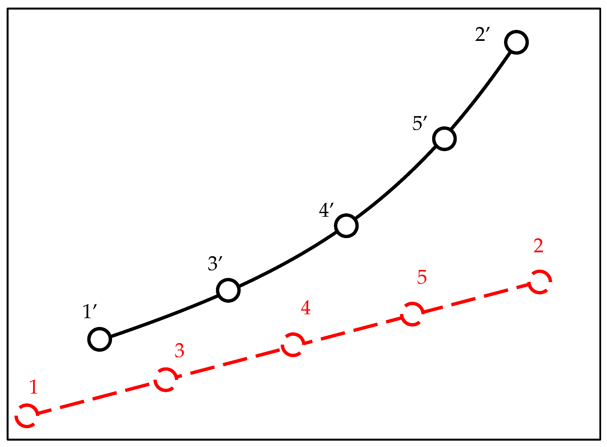
The second term (see Figure 3), which we designate as local displacements $\mathsf{\Delta }{u}^l$, results from an incremental displacement of the internal nodes, keeping the external nodal displacements (which for a beam include rotations) at zero.

$$\mathsf{\Delta }{u}^l=\left\{\begin{array}{c}0\\ \mathsf{\Delta }{u}_{ri}\end{array}\right\}$$

(6)

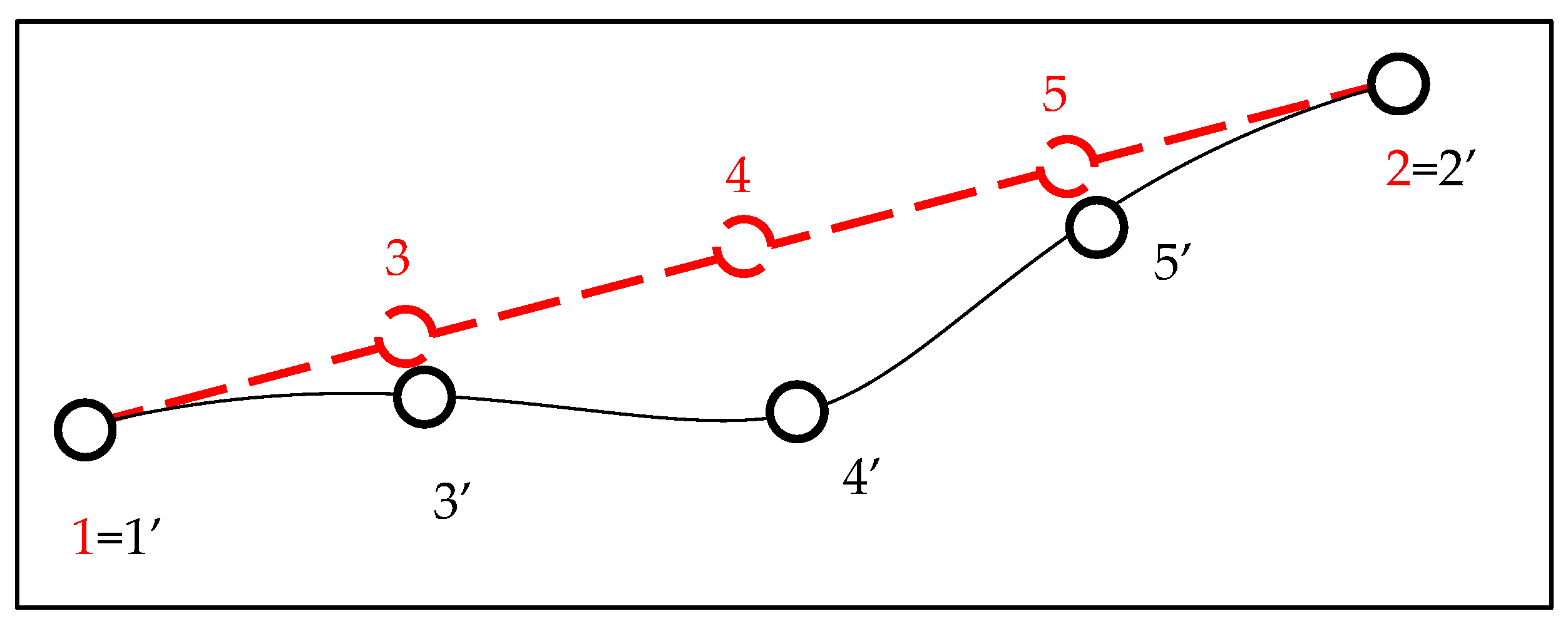
In Figure 4, we can see the total nodal displacements of the refined bar, $u_r$, obtained as the sum of the two terms mentioned above. We name $P$ the projection matrix that relates the refined nodal displacements to a reduced set of variables made up of the global amplitude $\eta$ and the internal nodal incremental displacements $\mathsf{\Delta }{u}_{ri}$.

$$u_r=\left. [\begin{array}{cc}{\varphi }_e& 0\\ {\left(K_{ii}\right)}^{-1}{K}_{ie}{\varphi }_e& I\end{array}\right]\left\{\begin{array}{c}\eta \\ \mathsf{\Delta }{u}_{ri}\end{array}\right\}=\left. [\begin{array}{cc}{\varphi }_e& 0\\ {\varphi }_i& I\end{array}\right]\left\{\begin{array}{c}\eta \\ \mathsf{\Delta }{u}_{ri}\end{array}\right\}=P\left\{\begin{array}{c}\eta \\ \mathsf{\Delta }{u}_{ri}\end{array}\right\}$$

(7)

where $I$ is the identity matrix.

We now solve the stability eigenvalue problem for this reduced set of variables and obtain a corrected critical load factor ${\lambda }_c \mathrm{a}\mathrm{s} \mathrm{f}\mathrm{o}\mathrm{l}\mathrm{l}\mathrm{o}\mathrm{w}\mathrm{s}$:

$${P^{T}K}_{r}P{\varphi }_c={\lambda }_c{P^{T}K}_{gr}P{\varphi }_c$$

(8)

Algorithm 1 shows the procedure used to calculate the corrected buckling load factor.

Algorithm 1. Calculation of the corrected critical load factor of a bar.

Calculate $K_r$ as a four-element refinement of the bar stiffness matrix;

Calculate $K_{gr}$ as a four-element refinement of the bar geometric stiffness matrix;

Calculate the projection matrix P in Equation (7);

Solve the projected eigenvalue problem in Equation (8) for ${\lambda }_c$.

Table 2. Relative error in critical load factor calculation with one element per member after applying the proposed correction.

Nel	CC	CP	PP	CM	CF
1	0.75%	0.45%	0.05%	0.05%	0.00%

displays the errors encountered in the critical load calculations after applying the correction process. The obtained results are deemed sufficiently accurate from an engineering perspective, notwithstanding the approximations employed.

The subsequent section outlines the extension of this correction process to structures with multiple bars.

4. Correction of Buckling Load Factor for Multiple-Bar-Element Frames

In order to generalize the procedure of the previous section to the case where the structure has more than one bar element, we introduce the following three basic ideas that will later be developed in detail:

• The local correction of the buckling shape that we applied in the previous section to a single bar can be applied sequentially to all the bars in the frame, thereby obtaining local improvements of the buckling shape inside each bar.
• The reduced modeling of the refined bar of the previous section can account for the stiffness and geometric stiffness of the whole frame by expressing all the nodal displacements outside the bar being corrected as the product of the frame buckling shape $\varphi$ times an amplitude variable $\eta$.
• The overall corrected frame buckling factor can be obtained by dividing the frame stiffness quadratic form by the geometric stiffness quadratic form calculated for the corrected buckling shape.

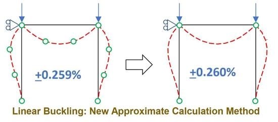
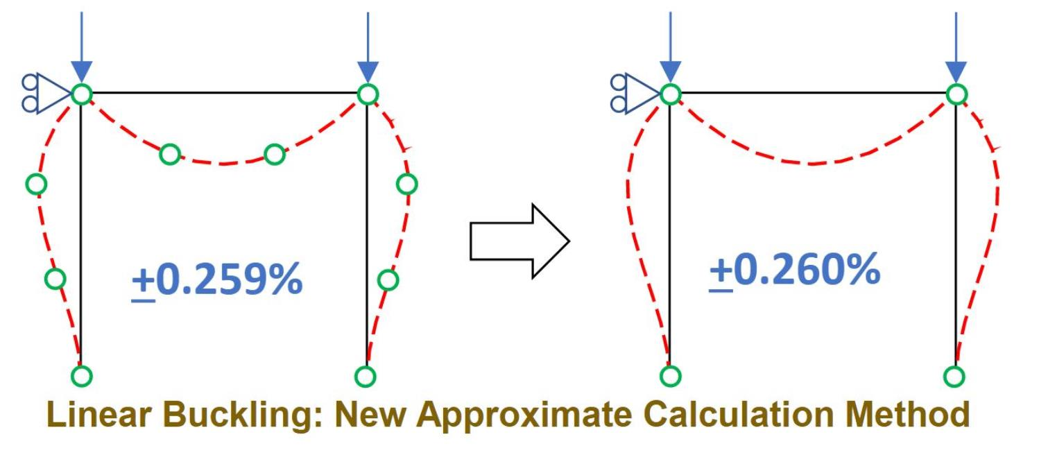
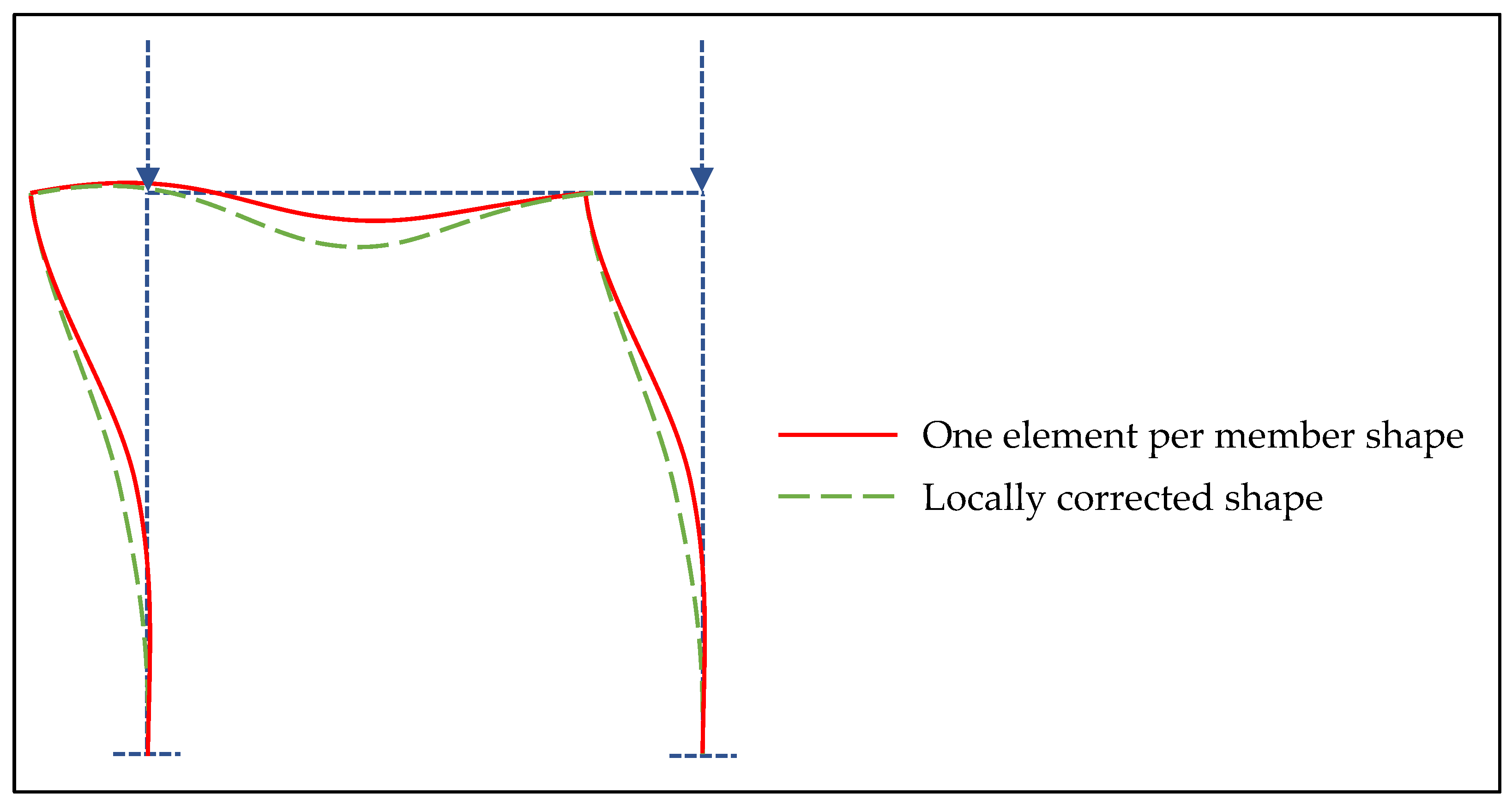
Figure 5 shows the buckling shape of a flat-roof portal frame subjected to two vertical loads calculated with a single element per member. After applying local corrections to the buckling shape inside each of the bars (that do not change the end nodal displacements of the bar), we obtain a locally corrected buckling shape.

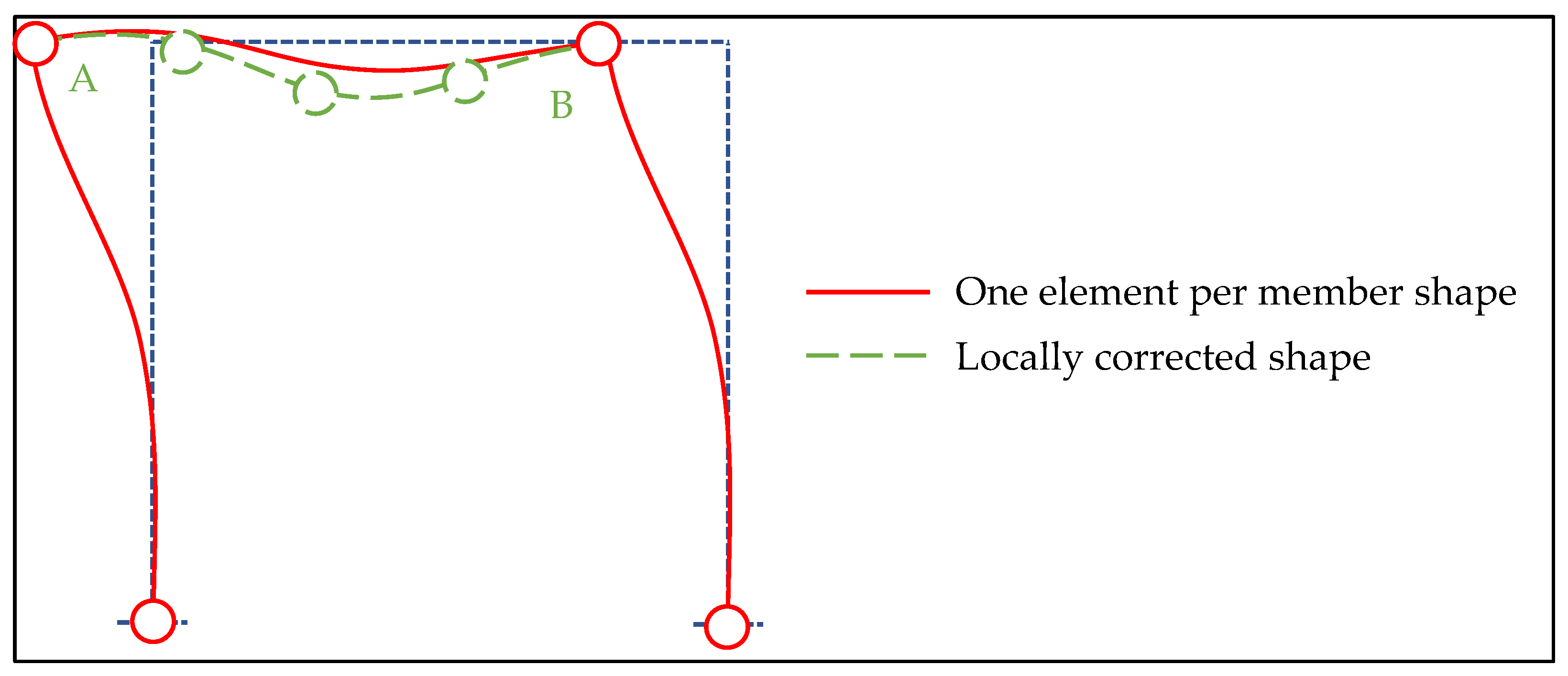
In order to calculate the local correction of the buckling shape for a certain bar, AB, we keep one-element discretizations of all the bars except the one being corrected, whose mesh we refine up to four elements (see Figure 6). It is important to note that the whole frame participates in the local correction of bar AB.

To calculate this local buckling shape correction, we need to solve an eigenvalue problem that we will develop next.

The quadratic form that is associated with the frame stiffness of the whole frame calculated with one element can be expressed as follows:

$$V=u^{T}Ku$$

(9)

where $u$ is the frame nodal displacement vector and $K$ is the frame stiffness matrix.

It does not change if we subtract and add the contribution of the bar being studied as follows:

$$V=u^{T}Ku-u_b^T{K}_b{u}_b+u_b^T{K}_b{u}_b$$

(10)

where $K_b$ and $u_b$ are the stiffness matrix and the nodal displacement vector of the bar calculated with one element.

Now, we can substitute the refined bar contribution for the one-element contribution as follows:

$$V=u^{T}Ku-u_b^T{K}_b{u}_b+u_r^T{K}_r{u}_r$$

(11)

where $K_r$ and $u_r$ are the refined bar stiffness matrix and nodal displacement vector (using four elements and five nodes). For the sake of convenience, we express $K_r$ and $u_r$ in the local coordinate system of the bar.

Now, we can express the nodal displacements in terms of a modal amplitude $\eta$ and the incremental internal nodal displacements of the bar being studied $\mathsf{\Delta }{u}_{ri}$, similarly to the actions we performed for a single bar.

$$u=\varphi \eta$$

(12)

$$u_b={\varphi }_b\eta$$

(13)

$$u_r=\left\{\begin{array}{c}{\varphi }_e\eta \\ {\varphi }_i\eta +\mathsf{\Delta }{u}_{ri}\end{array}\right\}$$

(14)

A similar procedure can be applied to develop a quadratic form for the geometric stiffness as follows:

$$V_g=u^T{K}_{g}u-u_b^T{K}_{gb}{u}_b+u_r^T{K}_{gr}{u}_r$$

(15)

Now, we can lay out the eigenvalue problem that we will solve to find the local buckling shape correction as follows:

$$K_c{\varphi }_{cb}={\lambda }_{cb}{K}_{gc}{\varphi }_{cb}$$

(16)

where

$$K_c=\left. [\begin{array}{cc}{\varphi }^{T}K\varphi -{\varphi }_b^T{K}_b{\varphi }_b+{\varphi }_r^T{K}_r{\varphi }_r& {\varphi }_e^T{K}_{ei}+{\varphi }_i^T{K}_{ii}\\ K_{ie}{\varphi }_e+K_{ii}{\varphi }_i& K_{ii}\end{array}\right]$$

(17)

$$K_{gc}=\left. [\begin{array}{cc}{\varphi }^T{K}_g\varphi -{\varphi }_b^T{K}_{gb}{\varphi }_b+{\varphi }_r^T{K}_{gr}{\varphi }_r& {\varphi }_e^T{K}_{gei}+{\varphi }_i^T{K}_{gii}\\ K_{gie}{\varphi }_e+K_{gii}{\varphi }_i& K_{gii}\end{array}\right]$$

(18)

$${\varphi }_r=\left\{\begin{array}{c}{\varphi }_e\\ {\varphi }_i\end{array}\right\}$$

(19)

$${\varphi }_{cb}=\left\{\begin{array}{c}{\varphi }_{ce}\\ {\varphi }_{ci}\end{array}\right\}$$

(20)

If we divide the corrected mode by ${\varphi }_{ce}$, we obtain

$${\varphi }_{cb}^{*}=\left\{\begin{array}{c}1\\ \frac{{\varphi }_{ci}}{{\varphi }_{ce}}\end{array}\right\}$$

(21)

So, we end up with a mode ${\varphi }_{cb}^{*}$, which is the sum of $\varphi$ and a local correction term $\mathsf{\Delta }{\varphi }_{cb}$, which only applies to the internal nodes of the bar being studied

$$\mathsf{\Delta }{\varphi }_{cb}=\frac{{\varphi }_{ci}}{{\varphi }_{ce}}$$

(22)

Now, we can calculate the corrected stiffness quadratic form for the bar, and the same for the geometric stiffness. We will use these quantities later to calculate the corrected load critical factor for the whole frame.

$$V_{cb}={\varphi }_r^T{K}_r{\varphi }_r+2\mathsf{\Delta }{\varphi }_{cb}^T{K}_{ie}{\varphi }_e+\mathsf{\Delta }{\varphi }_{cb}^T{K}_{ii}\left(2{\varphi }_i+\mathsf{\Delta }{\varphi }_{cb}\right)$$

(23)

$$V_{gcb}={\varphi }_r^T{K}_{gr}{\varphi }_r+2\mathsf{\Delta }{\varphi }_{cb}^T{K}_{gie}{\varphi }_e+\mathsf{\Delta }{\varphi }_{cb}^T{K}_{gii}\left({2\varphi }_i+\mathsf{\Delta }{\varphi }_{cb}\right)$$

(24)

In Algorithm 2, we show the steps to calculate the corrected quadratic forms of a bar in Equations (23) and (24).

Algorithm 2. Calculation of the corrected quadratic forms of a bar.

Receive as inputs one-element frame magnitudes ${\varphi }^{T}K\varphi$, ${\varphi }^T{K}_g\varphi$; Receive as inputs one-element bar magnitudes ${\varphi }_b^T{K}_b{\varphi }_b$, ${\varphi }_b^T{K}_{gb}{\varphi }_b$, ${\varphi }_b$;

Calculate $K_r$ as a four-element refinement of the bar stiffness matrix in bar reference frame;

Perform the same step for $K_{gr}$;

Transform ${\varphi }_b$ to bar reference frame as follows: ${\varphi }_e=R_b^T{\varphi }_b$ ($R_b$: bar rotation matrix);

Calculate ${\varphi }_i$, ${\varphi }_r$ in Equations (5) and (19);

Partition $K_r$ matrix according to external nodes (e) and internal ones (i) as follows: $K_{ee},K_{ei},K_{ie},K_{ii}$;

Perform the same step with $K_{gr}$, $K_{gee},K_{gei},K_{gie},K_{gii}$;

Calculate $K_c$, $K_{gc}$ in Equations (17) and (18);

Solve projected eigenvalue problem in Equation (16) for ${\varphi }_{cb}$;

Calculate corrected quadratic forms $V_{cb}$, $V_{gcb}$ by applying Equations (22)–(24).

After calculating the corrected quadratic forms for all the bars in the frame, the corrected load critical factor of the whole frame can be calculated as follows:

$${\lambda }_c=\frac{{\sum }_b{V}_{cb}}{{\sum }_b{V}_{gcb}}=\frac{{\mathrm{V}}_{\mathrm{c}}}{{\mathrm{V}}_{\mathrm{g}\mathrm{c}}}$$

(25)

where we define $V_c$ and $V_{gc}$ as

$$V_c={\sum }_b{V}_{cb}$$

(26)

$$V_{gc}={\sum }_b{V}_{gcb}$$

(27)

This corrected eigenvalue is better than the one calculated with one element per member, as we will see in the validation examples, but it can be improved in successive iterations in which we will replace the values of the modal stiffnesses of the bars ($V_b={\varphi }_b^T{K}_b{\varphi }_b$ and $V_{gb}={\varphi }_b^T{K}_{gb}{\varphi }_b$) with the corrected values ($V_{cb}$ and $V_{gcb}$). We can interpret that after calculating the corrected modal stiffnesses for each bar that depend on the neighboring modal stiffnesses of all the other bars in the frame, a better value will be obtained when we update the neighboring bar values with the modal correction. Therefore, we rewrite $K_c$ and $K_{gc}$ as follows:

$$K_c=\left. [\begin{array}{cc}{V}_c-V_{cb}+{\varphi }_r^T{K}_r{\varphi }_r& {\varphi }_e^T{K}_{ei}+{\varphi }_i^T{K}_{ii}\\ K_{ie}{\varphi }_e+K_{ii}{\varphi }_i& K_{ii}\end{array}\right]$$

(28)

$$K_{gc}=\left. [\begin{array}{cc}{V}_{gc}-V_{gcb}+{\varphi }_r^T{K}_{gr}{\varphi }_r& {\varphi }_e^T{K}_{gei}+{\varphi }_i^T{K}_{gii}\\ K_{gie}{\varphi }_e+K_{gii}{\varphi }_i& K_{gii}\end{array}\right]$$

(29)

Taking these ideas into account, we can redefine Algorithm 2 as follows (Algorithm 3):

Algorithm 3. Calculation of improved corrected quadratic forms of a bar.

Receive as inputs frame magnitudes $V_c$, $V_{cg}$; Receive as inputs bar magnitudes $V_{cb}$, $V_{cgb}$, ${\varphi }_b$;

Calculate $K_r$ as a four-element refinement of the bar stiffness matrix in bar reference frame;

Perform the same step for $K_{gr}$;

Transform ${\varphi }_b$ to bar reference frame as follows: ${\varphi }_e=R_b^T{\varphi }_b$ ($R_b$: bar rotation matrix);

Calculate ${\varphi }_i$, ${\varphi }_r$ in Equations (5) and (19);

Partition $K_r$ matrix according to external nodes (e) and internal ones (i) as follows: $K_{ee},K_{ei},K_{ie},K_{ii}$

Perform the same step with $K_{gr}$, $K_{gee},K_{gei},K_{gie},K_{gii}$;

Calculate $K_c$, $K_{gc}$ in Equations (28) and (29);

Solve projected eigenvalue problem in Equation (16) for ${\varphi }_{cb}$;

Update corrected quadratic forms $V_{cb}$, $V_{gcb}$ by applying Equations (22)–(24).

Now, we can write the iterative algorithm to calculate the corrected load critical factor of the whole frame as follows in Algorithm 4:

Algorithm 4. Iterative calculation of corrected load critical factor of whole frame.

Receive as inputs one-element frame magnitudes $K$, $K_g$, $\varphi$, $\lambda$; For all bars, receive as inputs one-element bar magnitudes $K_b$, $K_{gb}$, ${\varphi }_b$;

Initialize $V_c={\varphi }^{T}K\varphi$, $V_{gc}={\varphi }^T{K}_g\varphi$, ${\lambda }_c=\lambda$;

Perform    For b = 1:nbars;       If b is not in compression, go to End;       If first iteration, set $V_{cb}={\varphi }_b^T{K}_b{\varphi }_b$, $V_{gcb}={\varphi }_b^T{K}_{gb}{\varphi }_b$;       Update $V_{cb}$, $V_{gcb}$ with Algorithm 3;    End;    Update $V_c$, $V_{gc}$ with Equations (26) and (27);

Calculate ${\lambda }_c=V_c/V_{gc}$; While relative change in ${\lambda }_c$ does not fall below 0.01.

The algorithm can be optimized by correcting only those members for which the following is true.

$${\lambda }_c{N}_b^{comp}>N_b^{CF}$$

(30)

where $N_b^{comp}$ is the bar compression load and $N_b^{CF}$ is the bar buckling load when isolated from the frame and supported as a cantilever (case CF above).

$$N_b^{CF}=\frac{{\pi }^{2}E{I}_b}{{4L}_b^2}$$

(31)

The reason is that in these bars, the mode is less localized than in a cantilever (CF), and therefore, the modeling error in them is small.

We can also take advantage of the fact that the axial stiffness of the structural members is much higher than the other stiffnesses. Therefore, when calculating the corrected mode in each element, we can keep only the transverse displacements and their corresponding stiffnesses. In this way, the cost of the calculation is reduced.

It is interesting to note that the eigenvalue and eigenvector problems we are solving for each element use linear and geometric stiffnesses of the whole structure, and not just the element being corrected, although they project mostly to the element’s internal variables and to a single modal amplitude variable spanning the whole structure.

5. Results

5.1. 2D Building Portal Frame

Figure 7 shows a sample 2D building portal frame whose horizontal beams support distributed loads of 1 kN/m. The beams of the structure have an area of 40 cm², a moment of inertia of 1000 cm⁴ and a length of 4 m. The “exact” buckling load factor was calculated via Abaqus using 10 elements per member. The Abaqus calculation was also used to validate our program in Matlab, in which we coded the proposed novel algorithm. The buckling shape is shown in the same figure with red dashed lines.

The numerical results are shown in

Table 3. Corrected calculation statistics (2D sway portal frame).

Exact λ	1-Elem λ	Relative Error	Corrected λ	Relative Error
75.331	75.851	0.69%	75.351	0.027%

after one iteration and correcting 36% of the bar frames. The relative error is decreased by a factor of 30, although the one-element calculation is quite accurate in this case because it is a sway frame, and the buckling shapes are not localized.

Now, we repeat the calculation, restraining the horizontal displacement of each floor to prevent the side-sway frame failure as shown in Figure 8.

The numerical results are shown in

Table 4. Corrected calculation statistics (2D non-sway portal frame).

Exact λ	1-Elem λ	Relative Error	Corrected λ	Relative Error
217.33	373.10	71.67%	219.44	0.97%

after three iterations and correcting 57% of the frame bars. The relative error is decreased to an acceptable 0.97% by applying the correction. The one-element calculation is quite inaccurate in this case because the frame is non-sway and the buckling shapes are very localized.

We repeat the calculation using diagonal bars as a more realistic type of bracing, as shown in Figure 9, with similar results, as shown in

Table 5. Corrected calculation statistics (2D braced portal frame).

Exact λ	1-Elem λ	Relative Error	Corrected λ	Relative Error
227.11	408.79	80.00%	229.97	1.08%

.

5.2. 3D Stand Structure

Figure 10 shows a stand structure, taken from [9], that is made up of four columns, four horizontal beams and four slanted beams with one end at the top of each column, and the other at the highest point of the frame. On the highest point of the frame, there is a vertical load of 1 kN. The bars of the structure have an area of 40 cm² and an isotropic moment of inertia of 1000 cm⁴. The columns are 4 m high; the highest point lies at a height of 7 m, and the column bases are on the vertices of a 4 m sided square.

The “exact” buckling load factor was calculated via Abaqus using 10 elements per member. The Abaqus calculation was also used to validate our 3D program in Matlab, in which we coded the proposed novel algorithm. The buckling shape is shown in the same figure with red dashed lines.

The numerical results are shown in

Table 6. Corrected calculation statistics (3D stand).

Exact λ	1-Elem λ	Relative Error	Corrected λ	Relative Error
4655.4	4800.8	3.12%	4667.42	0.26%

after two iterations and correcting 67% of the bar frames. The relative error is decreased by a factor of 12. The one-element calculation error is low but not neglectable in this case because the side sway is not restrained and the buckling shapes are not localized.

5.3. 3D Building Structure

Figure 11 shows a sample 3D building structure which is made up of four portals, like the one we studied in the 2D example, laid out on planes parallel to xz. The portal horizontal beams support distributed loads of 1 kN/m, but the other horizontal bars do not, as is typical in building structures. The beams of the structure have an area of 40 cm², an isotropic moment of inertia of 1000 cm⁴ and a length of 4 m. The “exact” buckling load factor was calculated with our program using 10 elements per member. The buckling shape is shown in the same figure with red dashed lines.

The numerical results are shown in

Table 7. Corrected calculation statistics (3D sway building structure).

Exact λ	1-Elem λ	Relative Error	Corrected λ	Relative Error
74.336	74.889	0.74%	74.317	0.02%

after two iterations and correcting 25% of the bar frames. The relative error is decreased by a factor of 37, although the one-element calculation is quite accurate in this case because the frame is not braced and, therefore, the buckling shapes are not localized.

Now, we repeat the calculation using bracing diagonal bars, as in the 2D case, to restrain the side-sway failure in two orthogonal horizontal directions, as shown in Figure 12.

The numerical results are shown in

Table 8. Corrected calculation statistics (3D braced building structure).

Exact λ	1-Elem λ	Relative Error	Corrected λ	Relative Error
206.30	338.64	64.15%	207.08	0.38%

after six iterations and correcting 33% of the frame bars. The relative error is decreased to an acceptable 0.38% by applying the correction. The one-element calculation is very inaccurate in this case because the frame is non-sway, and the buckling shapes are very localized.

6. Discussion

The approach proposed by Xie and Steven [9], when applied to structures with multiple bars, requires the use of a weighted criterion that makes sense, but has less physical basis than the sum of the corrections from quadratic forms that we used here. Their method can be applied to calculate more than one eigenvalue, which is not strictly necessary to prevent the buckling failure of a structure. In addition, the structural members were discretized with more than one element in the cases presented.

Substructuring-based methods such as those in [12,13] require the calculation of the buckling modes of all bars in the substructure, while in the presented method, it is only necessary to do so for a fraction of them. Additionally, in their methods, it is necessary to condense the components retaining several modal amplitudes as variables for good accuracy, whereas when following our approach, only one mode per bar is calculated, if necessary.

Stiffness matrix condensation [17,18] is a very useful method for linear structural analysis or for incrementally solving nonlinear calculations, but it is not directly applicable to eigenvalue problems, although we have applied it as a part of the solution procedure.

The improved approximations of displacement and force fields presented by So and Chan [5] and Chan and Zhou [20], among others, give good results, but they are not generally compatible with beams modeled using the most common elements. The approach presented here is, in principle, applicable to any type of beam. It only requires the calculation of the local linear and geometric stiffness matrices of the subelements as well the buckling load of a cantilever used as a correction criterion. The latter can be replaced by an analytical value in many cases or calculated directly as a small-sized problem for the considered element.

The inclusion of flexible links [22], initial imperfections [21] and different types of loads [23,24] are topics of interest that would undoubtedly improve the quality of the results obtained and would be interesting to study in the future within the presented method.

Programs such as Abaqus suggest using several elements per beam/column member when carrying out a buckling analysis, whereas programs such as Staad, Sap2000, etc. suggest using two or three elements per member when the P-δ effects are relevant. The first approach means that a separate larger model should be used for the buckling analysis instead of the simpler one-element model of static analysis. The second approach involves an a posteriori experience-based judgment of the results of the buckling analysis to decide which elements should be refined. In addition, the methods used in these software packages to solve the eigenvalue problem are highly optimized but do not exploit the physical and topological properties of trusses, which can provide an additional increase in performance.

With respect to the efficiency of our method, the presented correction algorithm can be parallelized, and the local matrices of the refined bars’ subelements can be efficiently calculated either directly through a finite element formulation or by applying scaling factors to the transversal, torsional and axial submatrices of the one-element matrices. The calculation of the eigenvalues for the correction can be performed simply and efficiently, for example, by using the power method or any high-performance open domain software.

The analysis of the results reveals that the method is particularly advantageous for calculating non-sway structures, for which it is also possible to obtain accurate results for 2D frames by modeling the bar being studied and the stiffness of the neighboring bars [1,2,3], but in reality, it is not easy to know to what extent a structure is non-sway, and it may only be partially so. The proposed method solves this problem without relying on the sometimes-incorrect judgment of the structural engineer. Additionally, it allows for the solving of cases which are not perfectly sway or non-sway.

7. Conclusions

A new method was presented which makes it possible to calculate frame buckling loads accurately with the usual one-element-per-member models of structural elements that are common in commercial programs. Therefore, there is no need to use a model that is larger than the static one to calculate the critical buckling load. The method is easily parallelizable and is based on a correction of the overall buckling shape that affects only the inner degrees of the displacements of those elements where the compression loads are below the cantilever buckling load. As a result, one can take advantage of modern GPUs to perform the instability analysis at a fraction of the cost.

The method presented here models each structural member with a single element, which is then refined, if necessary, into four subelements, but it would be possible to use other combinations such as two elements per member and two refined subelements per primary element. In addition, the beam/column elements of the frame can, in principle, be of any type, even though the examples presented here only include cubic elements. This would make it possible to take advantage of a more descriptive modeling of the displacement field that would, in turn, require less demanding subsequent refinement.