1. Introduction
Graph theory is one of the main modeling tools used in biology [
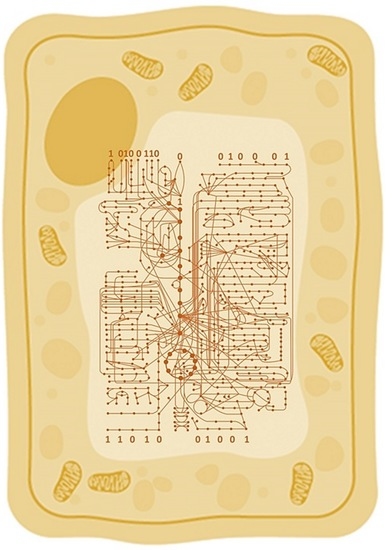
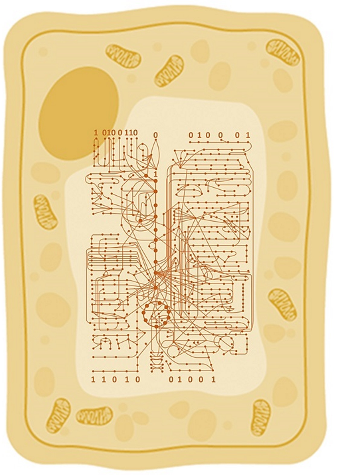
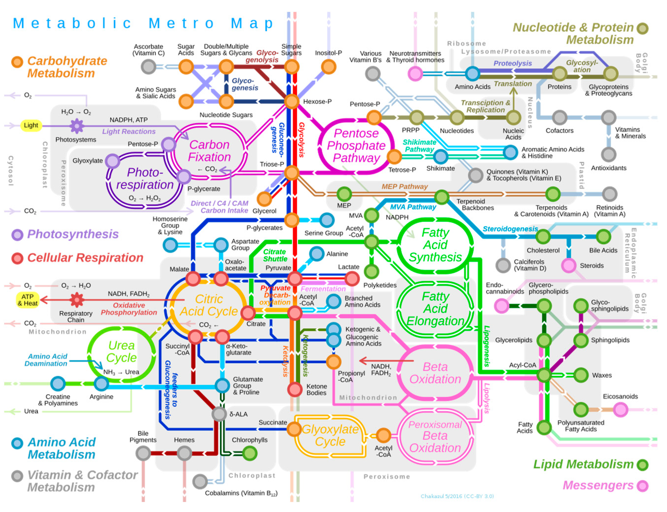
1] as it enables the mathematical analysis of networks composed of proteins, genes, transduction signals, metabolites, etc. As a modeling method, graph theory has provided, along with other modeling techniques, a procedure for the study of complex biological systems by means of a bottom-up approach. An example is the study of metabolic pathways (
Figure 1), i.e., the succession of biochemical reactions, where an initial substrate is transformed into one or more final products through a series of intermediary molecules or metabolites. The different reactions of all metabolic pathways are catalyzed by enzymes, i.e., by proteins that accelerate the rate of a reaction. In DNA, genes encode proteins, and since an enzyme is a protein, the expression of a gene results in an enzyme. Consequently, metabolism is ultimately governed by genetic control.
Graph theory is very useful in the analysis of complex systems consisting of objects connected to each other, e.g., metabolites. Therefore, through the use of graphs, we can model the biochemical transformations involved in a metabolic pathway. In graph theory, it is usual to represent a metabolic pathway as a directed graph in which the nodes represent the metabolic substances and the edges represent the biochemical reactions catalyzed by the enzymes. Thus, each of the enzymes involved in the metabolic pathway is identified by a label.
In agreement with [
2], the use of graphs in biochemistry dates back to 1949. However, the study of metabolic networks as dynamic systems ‘within organisms’ is an issue that is not straightforward to address [
3,
4]. The current view of metabolism is based on the consideration of two opposing approaches. On the one hand, [
5] views the metabolic network of an organism as a hierarchical organization of highly interconnected minor metabolic pathways. On the other hand, according to [
6], the metabolic network of an organism exhibits the characteristics of a small-world network model similar to computer networks, neural networks, and certain social networks. According to the latter approach, the biochemical reactions would be represented in the nodes of a graph and the metabolites in the connections between nodes.
Now, while a graph captures the structure of a metabolic network, its behavior can be studied by means of a system of ordinary differential equations that model the rates of change of the concentrations of the different metabolites comprising the metabolic pathway. Given a vector
S of metabolite concentrations and a vector
v of reaction rates (or quantity of metabolic substance that is transformed in a given biochemical reaction per unit of time), the equation that describes the system of equations modeling the behavior of a metabolic pathway is as follows [
7]:
where
N is referred to as the stoichiometric matrix, i.e., the matrix whose elements
nij represent the amount of metabolite
i formed in reaction
j. Therefore, a metabolic network can be represented either as a graph or as a stoichiometric matrix (
N-matrix), the latter representation being equivalent to a hypergraph [
8].
In this paper, using a simulation model we studied how each of the enzymes involved in a metabolic pathway could evolve during the course of Darwinian evolution, thereby, how the arcs or edges of a graph connecting one node (metabolite) to the next in a metabolic pathway evolved. In summary, how did metabolism evolve to yield today’s metabolic networks?
There are currently two hypotheses (
Figure 2) about how metabolic networks could have evolved [
9,
10]. One of these hypotheses, known as the ‘retrograde model’, postulates that when a metabolite that acts as the substrate
Sy of a metabolic reaction catalyzed by an
EB enzyme is depleted, then the
EB enzyme evolves, resulting in an
EA enzyme that precedes it, catalyzing the reaction that will produce the depleted substrate
Sy. In contrast, the hypothesis that is referred to as the ‘patchwork hypothesis’ conjectures that primitive enzymes were quite unspecific, catalyzing the transformation of a wide range of metabolites or substrates. Over time, these nonspecific enzymes would have evolved into other specialized descending enzymes. It is now believed that this hypothesis could explain the topology of the metabolic networks of living organisms.
In order to be able to answer this question, we assume that a metabolic network is a (a) dynamic system whose (b) structure is represented by a graph, studying through simulation the emergence during the evolution of the different enzymes involved in the catalysis of metabolic reactions. Likewise, in the graph depicting a metabolic pathway, (c) nodes represent the molecules or metabolites, and (d) arcs or edges represent the chemical reactions mediated by enzymes.
Of the set of metabolic pathways present in living organisms (
Figure 1), we have chosen two of the most representative metabolic pathways: glycolysis and the Krebs or tricarboxylic acid (TCA) cycle. These are two metabolic pathways of great evolutionary significance in living organisms. Glycolysis is an ancestral metabolic pathway, i.e., one of the oldest in evolution, responsible for the oxidation of glucose into pyruvic acid. The result is the production of energy in the cell, and this metabolic pathway occurs in both oxygen-breathing and non-oxygen-breathing organisms. In oxygen-breathing organisms, the pyruvic acid resulting from glycolysis will undergo a series of chemical transformations in the so-called Krebs cycle or TCA cycle. The purpose of this cycle is to continue the oxidation of the metabolic intermediates, with the electrons from this oxidation being captured by citric acid, again resulting in additional energy for the cell. The final balance is the production of energy from glucose in the form of three molecular species (4 ATP, 10 NADH, and 2 FADH
2).
Finally, and although this is an additional matter for the purpose of this paper, we also simulate the evolution of the enzymes involved in the alcoholic fermentation pathway because of their importance in the biotechnological industry.
2. Materials and Methods
2.1. Simulating Evolution with a Genetic Algorithm
Genetic algorithms (GAs) are stochastic optimization methods inspired by the principles of natural selection [
11] established by Darwin’s evolutionary theory in 1859. Currently, they are used in optimization and search problems, being trial-and-error methods in which the solution space is continuously explored and evaluated until an optimum (global or local) is found. The search for an optimum simulates the survival of the most valid solutions or “individuals” in an environment or “problem space”. Since they were introduced by Holland [
12] and popularized by Goldberg [
13], GAs represent today one of the most widely used optimization techniques in the field of Artificial Intelligence (AI) due to their many applications in engineering, market research, commerce, operations development, biology, sociology, game theory, computer science, etc. [
14].
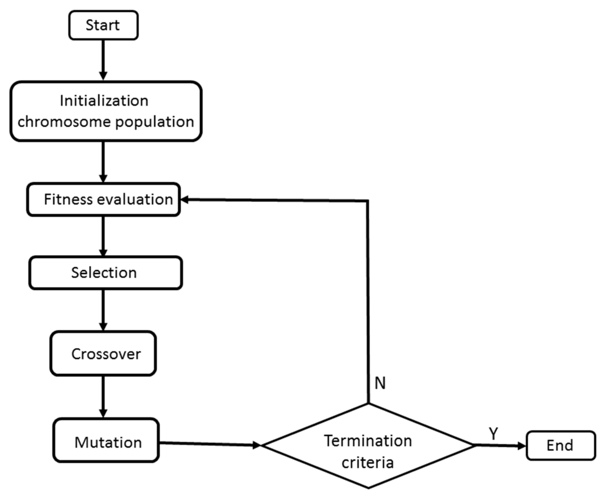
A GA involves the following steps or stages (
Figure 3). First, (a) a set of solutions (individuals) is randomly generated. Individuals are represented by a vector that models the chromosomes, that is, the structure storing the genetic information (DNA) of a living being. In the present model, chromosomes were defined as binary strings. Afterward, (b) the fitness of chromosomes, goodness or validity of the solutions—a metaphor of adaptation to the environment—is evaluated. Those solutions with a higher fitness value will have a higher probability of surviving and, therefore, of passing to the next generation (gene propagation). The solutions that pass to the next generation will experience the effect of genetic mechanisms, in particular (c) mutations and genetic crossover, which are simulated in the GAs. The goal of these genetic mechanisms is to introduce variability in the population or set of solutions by promoting the search for new solutions. The search process is repeated over and over again until (d) an optimal solution is found.
The search for new solutions, i.e., the exploration of the problem space, is the result of the simulation of mutation and crossover or recombination. In a GA, these mechanisms are simulated by means of the so-called genetic operators. In the present work, we have used the recombination operator at one point and the mutation operator for chromosomes defined as a binary string (flip-by-bit method).
According to
Figure 4a, the one-point recombination was implemented as follows. Once the two parental chromosomes are chosen, a cutoff point is randomly selected, i.e., in the present example, at the second position, and the chromosome segments are then exchanged. The result of this mechanism is an offspring consisting of two recombinant chromosomes as they share the information of the parental chromosomes. A value of the
pr recombination rate is set at the beginning of the simulation experiment.
Mutation was simulated (
Figure 4b) by randomly choosing one of the offspring chromosomes, e.g., the right one. Next, we randomly selected two positions, for example, the first and the fifth, flipping the value of the binary number (0 → 1, 1 → 0). In a manner similar to recombination, the population mutation rate
pm is set at the beginning of the simulation experiment.
Simulation experiments were conducted using a simple genetic algorithm, SGA, customizing the algorithm to the goals of the present model. The code in Python language is available in [
15].
2.2. Vectorization: Binary Representation of Metabolites
The first step in GA is to initiate the population or set of solutions, in our case, the enzymes that will transform one metabolite into another in a metabolic pathway. In the present paper, the formal representation of enzymes and metabolites is referred to as vectorization. Metabolites are molecules, and vectorization was performed as binary matrices according to the method developed in [
16].
In the present model, the nodes represent the metabolic intermediates, i.e., sugars and other glycolytic molecules. It is important to note that the representation of a molecule of metabolism as a binary matrix is actually not a new approach, but the criterion adopted in this work is a novelty differing from the usual approach.
In 1974, ref. [
17] translated the molecular topology into a matrix, taking an element
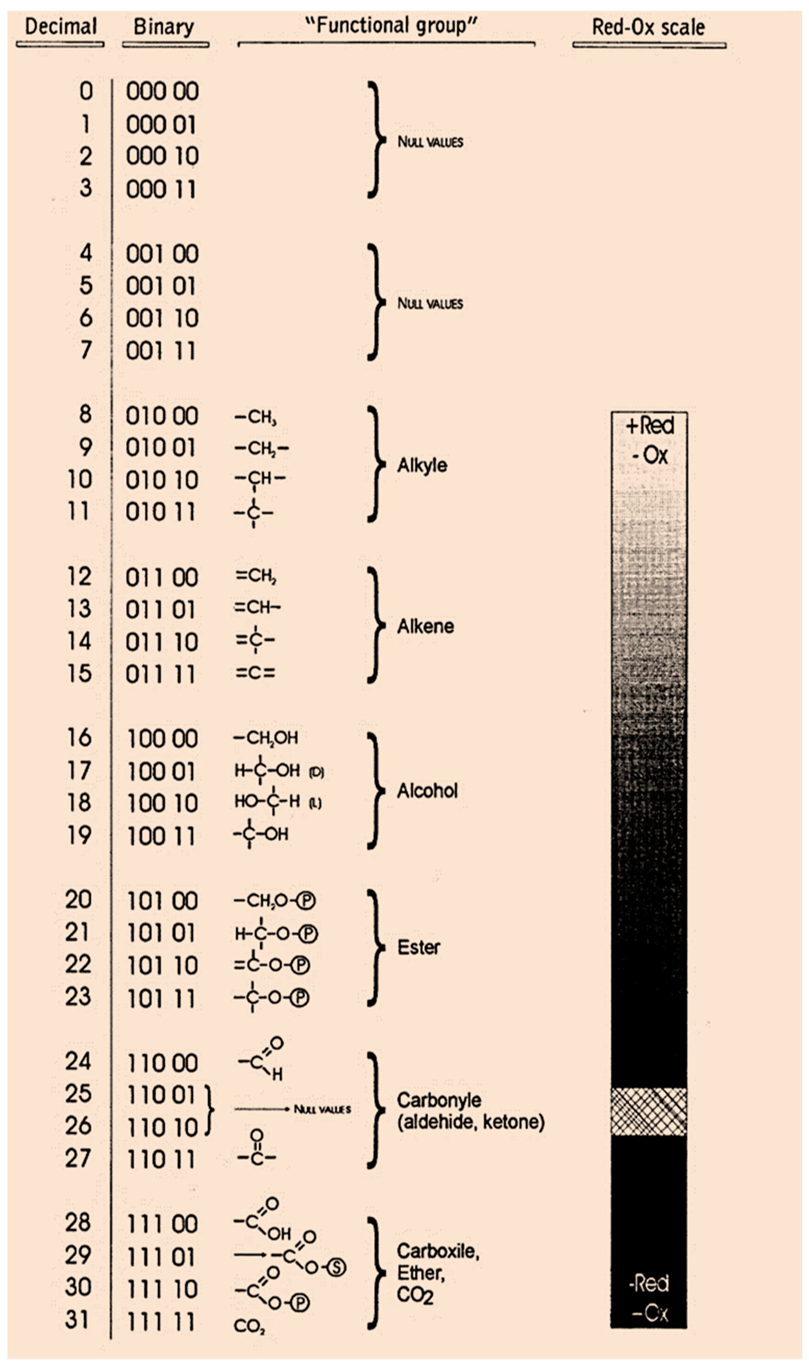
aij with the value of 1 when the edges are adjacent or 0 otherwise. However, unlike this procedure, the method we have followed in this work assigns a 5-bit word to the functional groups of the molecule. To this end, we defined a table or “Rosetta stone” of cellular metabolism. According to
Figure 5, we assigned a 5-bit word to each functional group (group of atoms in a molecule with distinctive chemical properties), ordering the most frequent functional groups in the metabolic intermediates depending on their redox potential (the tendency of a functional group to acquire electrons). Note how the vectors were classified by their redox potential from the most reduced form corresponding to the alkyl group to the most oxidized form represented by CO
2.
In accordance with the above, the substrate
S and the product
P of a biochemical reaction catalyzed by an enzyme
E were encoded in a matrix whose elements are zeros or ones [
16]. It is interesting to note that all metabolites
Mix5 in glycolysis and the Krebs cycle are molecules with
i equal to 3, 4, 5, or 6 carbons. Thus, depending on the number of carbons in the molecule, we will represent a metabolite as follows:
It is important to indicate that given a value
i, the row vector
ai1,
ai2,…, a
i5 represents a functional group, either of the substrate
si5 or product
pi5. That is, each row of any of the above matrices represents a carbon atom of the molecule, providing that, according to
Figure 5, a total of thirty-two possible binary vectors (from 00000 to 11111). However, since Krebs cycle metabolites are the result of the arrangement of twenty-two functional groups, then the ten binary vectors in
Figure 5 are chemically meaningless for Krebs cycle metabolites. In the present work, in order to conduct simulation experiments including CO
2 and acetyl-CoA molecules, both molecules were modeled as a row vector
v and an
M2×5 matrix:
2.3. Modeling an Enzyme as Automaton
Once the metabolite molecules were represented as binary matrices, the enzymes that catalyze the transformation of one metabolite into another were modeled as automata.
Enzymes are proteins with catalytic properties that can increase and regulate the reaction rate. In this work, and as already mentioned above, we simulated the evolution of the enzymes and, subsequently, of the appearance or emergence of each of the arcs of the graph representing the metabolic network.
Since enzymes are proteins, unlike metabolites, which are sugars, their vectorization does not represent their chemical composition. An enzyme has the organization depicted in
Figure 6. The region of the enzyme where the substrate binds is called the active site, is the place where the chemical reaction occurs. The conformational state of the active center is the molecular shape of the enzyme in the active center. Therefore, the conformational state determines the affinity between the enzyme and the substrate. Assuming an analogy to the key-lock concept, the active center of the enzyme would be the lock and the substrate the key. Once the substrate
S binds to the active center of the enzyme
E, and then the substrate is transformed into a product
P by breaking and forming chemical bonds:
In (4), the amino acids, i.e., the basic building subunits of proteins, are responsible for the transformation of the substrate S into the product P of the reaction. From a biochemical point of view, these amino acids create an environment in the active center with different chemical characteristics (hydrophobic or hydrophilic, acidic or basic). Furthermore, temperature and pH can affect the enzymatic reaction, although this fact has not been included in the present model.
The role of enzymes is of such importance in biochemistry that they have frequently been the subject of study and computer simulation using a wide repertoire of modeling and simulation techniques. Whether using the Michaelis–Menten differential equation, the Monte Carlo method, a molecular dynamics method, or the cellular automata approach, all of these techniques have attempted to capture the primary function and features of the enzymes. In the present work, we have modeled enzymes as automata [
18].
Cellular automata are discrete space and time models that have been used to model biological systems [
11]. A cellular automaton in two dimensions (
D = 2) is a checkerboard where each cell is called a “finite automaton” because the cell is in any of a finite number of states. The state of a given automaton
St(
x) located at cell
x at time
t changes depending on the states of neighboring automata
St(
x+
x0),
St(
x+
x1),…,
St(
x+
xn−1) by applying a state transition rule (5) to update its state [
11,
19]:
Applying this approach, enzyme kinetics have been modeled on several occasions [
18,
20,
21,
22], including the simulation of metabolic networks, for instance, the mitogen-activated protein kinase signaling cascade [
23], the hypothetical unidirectional network of enzymatic reactions studied by [
24], etc.
In the field of molecular biology, the technique of cellular automata has been successfully used to simulate the dynamic activities inside cells. For example, this technique was useful in the 1990s, enabling the construction of simulation models in structural biology in which the dynamic behavior of the system being simulated was mediated by enzymes and/or polymerization and self-assembly phenomena [
25]. This technique enables the construction of models, solving many of the limitations of classical differential equation models, such as the 3D graphical representation of a system composed of different classes of molecules. An example is the model [
26] in which, using molecular automata, it was possible to simulate
Escherichia coli membrane assembly, the operation of ATP synthase as well as the assembly of the bacterial flagellar motor.
Electronic Enzyme Model
Enzymes were modeled as automata according to a class of automata introduced by [
27], referred to as electronic enzymes. The electronic circuit modeling of an electronic enzyme is a hardware-level model of the active center of an enzyme, which is configurable via a genetic algorithm (see
Section 2.1). The possible applications of this class of hardware were patented [
28].
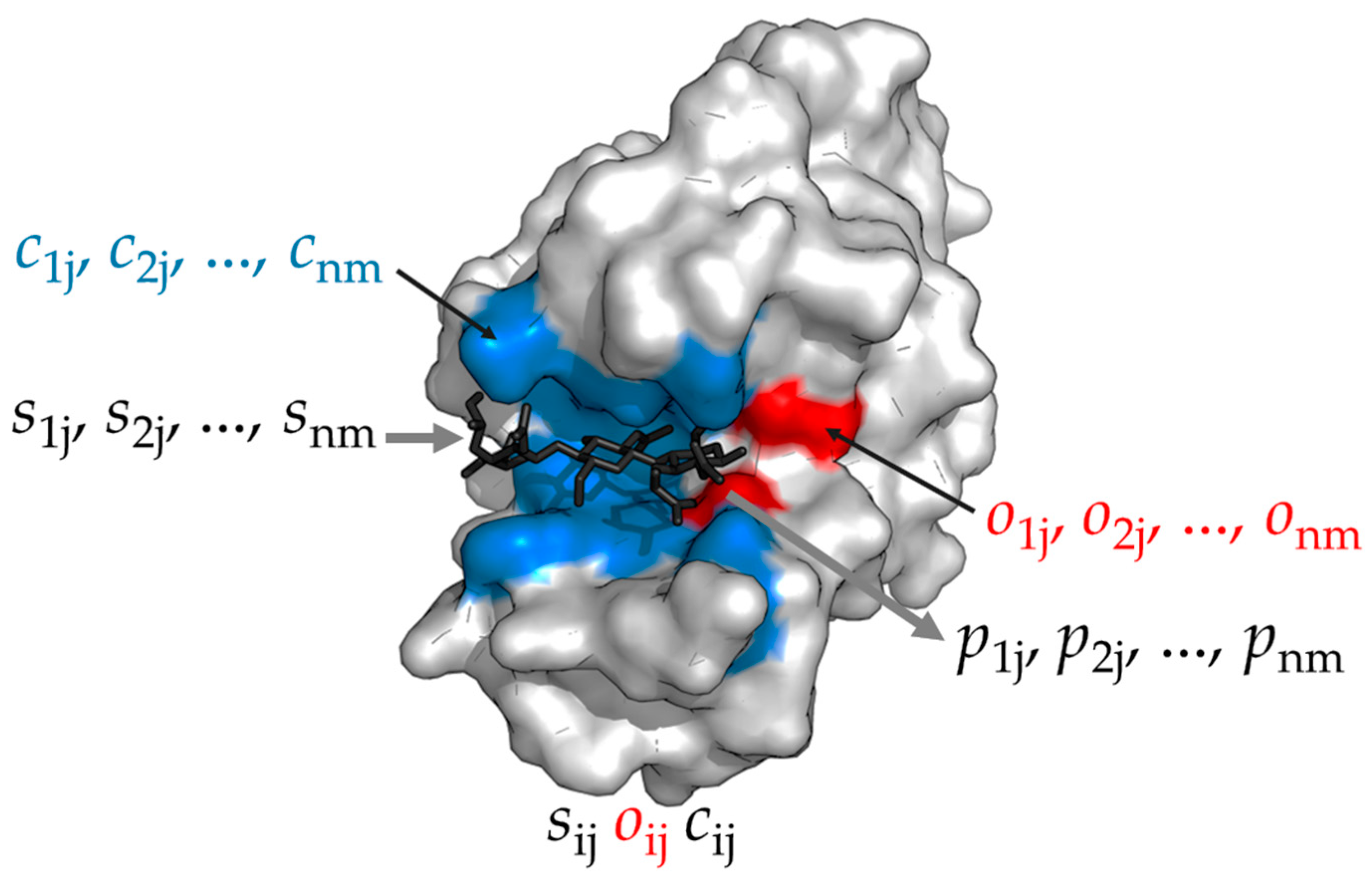
We define this kind of automata as follows. An electronic enzyme
Em is a vector resulting from concatenating two strings of
n bits length, respectively:
where
c1j,
c2j,…,
cnm is an
n-bit string (
i = 1, 2, …,
n) representing the ‘conformational state’ of the enzyme
Em (
j = 1, 2, …,
m). Thus, in the active center then
n-bit string would be defining the binding sites and substrate orientation (
Figure 6). In addition,
o1j,
o2j,…,
onm are the Boolean operators AND (
oij = 1) or XOR (
oij = 0) modelling the amino acids of the active center that are involved in the reaction which converts the substrate
S into a product
P. As a consequence, the
n-bit string
o1j,
o2j,…,
onm would define the ‘catalytic site’ of the active center of the enzyme (
Figure 6).
According to the
Em definition, an enzymatic reaction, i.e.,
Sm +
Em →
Pm, is a transformation rule defined by the following logical operations:
where
sij and
pij are the substrate and product resulting from the reaction (4).
For example, let 1110 be the substrate S (i = 4) and E be the enzyme (of reaction j) defined by 10101000. In this example: p1j = 1 AND 1 = 1, p2j = 1 XOR 0 = 1, p3j = 1 XOR 1 = 0, p4j = 0 XOR 0 = 0, being the product P obtained from the reaction is 1100.
2.4. Binary Model of Glycolysis and Krebs Cycle
Applying the concepts and definitions described above, the glycolysis pathway was modeled, as shown in
Figure 7. Likewise, using the same methodology, the Krebs cycle was modeled as has been depicted in
Figure 8.
2.5. Simulating the Evolution of the Metabolic Pathway of Alcoholic Fermentation
After the simulation of glycolysis and Krebs or TCA cycle evolution, an additional experiment was conducted to simulate the evolution of the enzymes involved in the metabolic pathway known as alcoholic fermentation. Alcoholic fermentation is the metabolic pathway carried out in yeasts and some bacteria that is applied as a biotechnological process to convert sugars into ethyl alcohol and carbon dioxide.
We simulated the metabolic pathway illustrated in
Figure 9, where each reaction is catalyzed by E17, E18, and E19 enzymes, respectively.
2.6. Simulation Experiments
The enzymes Em were defined as 10-bit vectors, the first 5 bits being the conformational state and the remaining 5 being the Boolean operators. The optimal binary string of the vectors modeling the substrates is searched evolutionarily via a genetic algorithm. An enzyme will be optimal if it is satisfied that the transformation of one or more of the rows of the matrix representing the substrate results in the reaction product matrix corresponding to a step within a metabolic pathway.
In the present article, we have omitted for simplicity the name, properties, and detailed explanation of the mechanism of action of the enzymes E involved in the biochemical reactions because the interested reader will find this information in any general biochemistry textbook.
From the set of matrices modeling the intermediates of glycolysis and Krebs cycle, the initial population (t = 0) was obtained according to the following method.
An initial population P(0) consisting of 100 enzymes (binary chromosomes of 10-bit length) was obtained with a random number generator U [0, 1] with uniform distribution. The population P(t) will evolve during 200 generations such that once the 200th generation is reached, the genetic algorithm ends, obtaining the optimal solutions or chromosomes and, therefore, the optimal enzyme configurations. In each simulation experiment, 100 replicates were conducted, and since it is a stochastic optimization method, more than 2,000,000 solutions or enzymes were obtained from the initial population P(0).
Based on the
P(0) population of randomly generated chromosomes, reproduction, recombination and mutation were simulated by means of a genetic algorithm. In each generation, the configuration of the enzymes was evaluated, and its fitness value
fE was obtained according to the following evaluation function:
In the above function (8), indexes i, k represent the rows and j the column in the matrix S, is a coefficient whose value was 100 in the simulation experiments, is equal to the term, and l is the chromosome length. Thus, the enzyme fitness value is calculated by simulating the enzyme–substrate reaction (4), i.e., the operation between substrate and enzyme (7), and then comparing the product obtained from the reaction with the target product , i.e., the substrate of the next step or reaction of the metabolic pathway. The similarity between the obtained product and the target product or next substrate was calculated using the Hamming distance . The Hamming distance is the number of positions in which two binary vectors or matrices with identical length or number of rows and columns differ, respectively. For this purpose, the chromosomes were decoded, resulting in the configuration of each enzyme, i.e., the conformational state (c1j, c2j,…, cnj) and the catalytic site (o1j, o2j,…, onj) involved in the reaction.
Note that the genetic algorithm that simulates Darwinian evolution finds the appropriate configuration of the active center of an enzyme when the sum of the fitness function is zero. Then, once the chromosomes were evaluated, the new generation of chromosomes was obtained by applying the wheel parents selection algorithm [
11]. In the chromosomes of the new generation, genetic variability is simulated through the genetic mechanisms of recombination and mutation. As explained above, recombination was performed with the one-point recombination operator, and mutation was simulated by applying the mutation operator based on the flip-by-bit method.
Based on the described methodology and using the fitness function (8), we conducted simulation experiments to find the optimal configurations of the enzymes involved in the metabolic pathways of glycolysis, Krebs cycle and alcoholic fermentation. The experiments were performed by assigning the following parameters in the SGA: population size N equal to 100 enzymes, maximum number of generations Gmax equal to 200, number of replicates r per experiment equal to 100, recombination rate pr = 0.20, mutation rate pm = 0.01 (rate of change of the bit value pb = 0.05).
Once the results of the simulation experiments were collected, the average fitness of each generation was calculated, obtaining the performance graph of the genetic algorithm. In addition, an
MB molecular biodiversity value (in bits) was also obtained for the optimal enzymes (see
Appendix B,
Table A1) by applying the following expression:
where
n is the total number of optimal enzymes, and
n1,
n2,…,
nk is the number of different molecular forms of the enzyme. Thus,
n is the number of enzymes with the same conformational state and catalytic site found by the genetic algorithm, and
nk is the number of enzymes of class
k. In expression (9) the factorials were approximated by Stirling’s formula.
Since the different molecular forms (1, 2,… k) of the enzymes share a common catalytic activity they are called isoenzymes. Therefore, the above formula is a measure of molecular biodiversity, i.e., the richness and number of different enzymes catalyzing the same biochemical reaction.
3. Results
The obtained results suggest that the simulations conducted capture essential elements in the evolution of metabolic pathways, and in particular, those related to intermediary carbon metabolism.
Figure 10 represents in a graph and using binary notation the flow of information in bits that would take place in a ‘digital electronic circuit’ that would be the hardware implementation of the central carbon metabolism, i.e., glycolysis and Krebs cycle. In
Figure 11, we illustrate the classical performance graph of a genetic algorithm, thereby proving at the simulation level the Darwinian evolutionary convergence of enzymes in a hypothetical organism.
Table A2 and
Table A3 (
Appendix B) show the results obtained in the simulation of glycolysis and Krebs cycle, respectively.
Similar results were obtained for the evolution of the metabolic pathway of alcoholic fermentation.
Table A4 (
Appendix B) shows the results of the metabolic pathway of the simulated fermentation in yeast.
In addition, it is interesting to note that the Boolean operations modeling the catalytic site of the enzymes have an associated cost. The cost was expressed as energy consumption, penalizing the presence of XOR gates in the active center in the fitness value of the enzyme. Hence, in the simulations, whereas for the AND gate, the cost was equal to 1, the cost for the XOR gate was 1.5. In these simulation experiments, the result was a decrease in the biodiversity of optimal enzymes, emerging along the evolutionary pathway only those enzymes with the lowest cost and, therefore, with the lowest energy cost. We found only eight enzymes that included the XOR operator in their active center. However, in the general experiments where this restriction is not present in the fitness calculation, we obtained 54 optimal enzymes capable of catalyzing the biochemical reaction, despite the fact that their active center includes a greater number of XOR operators.
4. Discussion
From the simulation experiments conducted with the evolution of glycolysis, Krebs cycle and alcoholic fermentation networks, we can conclude that Darwinian evolution is able to optimize a biological network, such is the case of a metabolic network. However, in our study, the evolution of the enzymes involved in a metabolic network is not simulated by taking into account the stoichiometry of the reactions and the kinetic parameters of the enzymes. Although the latter is the usual protocol, it has not been the case in the present work. In our model, the evolution of the enzymes, and therefore of the edges of the graph representing the metabolic network under study, is simulated with the assumption that the active center of an enzyme can be modeled as an automaton. This approach is one of the main novelties of the present paper.
Now, what does graph theory contribute to our understanding of the evolution of metabolic networks in living beings? According to [
3,
29] and in a similar manner to many complex non-biological systems, metabolic networks exhibit characteristics that are typical of small-world networks. For example, they exhibit a power-law degree distribution, high cluster coefficients (a feature of robust networks being metabolic networks resilient to damage) and small network diameter (close distance between metabolites). These characteristics would be a consequence of the way in which biochemical reactions have been assembled with each other under the Darwinian mechanism of natural selection. Obviously, this assembly between reactions, i.e., the connection between the nodes (metabolites) of the graph (metabolic networks), is embodied by the evolution of enzymes. Thus, the evolution of the enzymes involved in the catalysis of the biochemical reactions (edges of the graph) transforms one metabolite (node) into the next. This point of view would be in agreement with the model [
30] that describes the evolution of a metabolic network as a Markov process in which the insertion and deletion of reactions take place. The above approach is plausible since the survival of an organism depends on the characteristics exhibited by its metabolic networks. In this sense, the production of energy is crucial for a living organism. For example, the transformation of the most important sugar, glucose, into energy in the form of the ATP molecule was a critical step in the evolution of life on Earth. Thus, evolution allowed the optimization of the glycolytic pathway [
31] by adopting the maximum production of ATP as the principle of optimization.
However, the above view about the evolution of metabolic networks contradicts the view of [
6], observing that most important metabolic networks in an organism, i.e., glycolysis, Krebs cycle, and the pentose phosphate cycle, are distributed or split into different subsets or modules. These modules would represent the functional units of metabolism. In the case of the TCA or Krebs cycle, this modularity may be a consequence of the fact that TCA is the largest metabolic cycle found in organisms [
4]. Consequently, and according to [
32], the large network that forms the metabolism could be broken down into modules: the metabolism is organized around several core modules that interact strongly with each other, being responsible for the basic functions of metabolism. These central modules would interact in turn with other peripheral modules responsible for relatively independent metabolic functions. In other words, and according to [
32], there would be a correlation between function, evolution, and topological modularity. which would suggest that the architecture of metabolic networks is a result of their evolutionary history.
Nevertheless, and with respect to the two previous approaches, small-world versus modularity, there are opinions [
33] on the extent to which the properties of metabolism deduced by applying graph theory really reflect the biological organization present in living beings or, on the contrary, are merely an artifact resulting from the graph representation. Of course, methodologies other than graph theory can be applied. For example, glycolysis can be modeled and simulated with differential equations [
34] or graph theory using Petri nets [
35]. Alternatively, as we have undertaken in this work, we can use automata theory, e.g., electronic enzymes or, inspired by artificial neural networks, we could also use for this purpose the so-called ‘biochemical neurons’ [
36]. However, no matter the method used, the simulation of the evolution of a metabolic network is a complex problem that, in many cases, will lead to queries similar to [
33].
In the field of biology, answering the question of how the evolution of enzymes involved in glycolysis and the Krebs cycle could have taken place is still a matter of debate. At present, there is still a debate between the retrograde model and the patchwork model [
9,
10], although there are classical papers that support the results of our work. In particular, ref. [
36] argues that the glycolytic pathway appears to be the result of the chance assembly of independent evolved enzymes. Indeed all glycolytic enzymes are variations with a common motif: they all have a core of
-sheet protein chains surrounded by
-helices chains. However, although the experimental data are important, perhaps the most satisfactory explanation comes from theoretical biology. During the 1990s, studies were carried out in which the evolution of a metabolic pathway was considered to be an optimization problem, as has been addressed in the present paper. For example, refs. [
37,
38] found in a model known as the ‘pentose game’, whose results apply to the evolution of the Krebs cycle, that the evolution of a metabolic pathway must satisfy certain requirements. These requirements were included under the common term of simplicity. The simplicity principle was summarized in a simple idea: the metabolite production occurs by the shortest route and, therefore, with the smallest possible number of reaction steps. Therefore, although the molecular biodiversity of the number of optimal enzymes we have calculated with (9) is so high; ultimately, living beings operate with only a few enzymes. This is because principles such as the simplicity principle we have just enunciated, which are a consequence of Darwinian natural selection, impose a strong constraint on the selection of a few enzymes.
The study of biological evolution is a problem that requires powerful mathematical and computational tools. In the particular case of the evolution of metabolic pathways, graph theory is useful for both studying the structures [
39] present in organisms as well as for the analysis of the dynamic processes exhibited by living organisms [
40]. Moreover, the application of graph theory together with heuristic methods such as genetic algorithms [
41] is a promising approach to the study not only of metabolic networks but also complex networks. Complex networks are not easy to study because they behave as dynamic systems that evolve and change over time, e.g., social networks, the brain, the Internet, the immune system, electric power distribution networks, insect colonies, etc.
This paper is an example that illustrates a common problem in biology. In many biological studies, it is not enough to have powerful computers and sophisticated mathematical modeling tools, as is the case of graph theory. In many cases, the problem is the lack of solid working hypotheses, assumptions, and, therefore, of a proper experimental framework that would make it possible to search for satisfactory answers. Consequently, and to date, we still do not have a satisfactory ‘picture’ or global model to explain how the evolution of metabolism took place. However, despite these limitations, the study of the principles of the evolution of metabolic networks can be approached through simulation experiments, i.e., under a computational paradigm or framework [
42]. Thus, experiments could be conducted in silico with a representation in a simplified form of the main components of biochemical reactions such as enzymes, fitness function, metabolites and even genes. The results of the simulation experiments [
42] or those obtained by us in this paper would be congruent with the patchwork hypothesis (
Figure 2), i.e., modern and highly specific enzymes would come from ancestral enzymes less specific in recognizing a substrate or metabolite.
Although our results may shed light on the evolution of metabolism, it is the methodology we introduce here that represents a novel contribution within the so-called computational paradigm. Nevertheless, this paradigm is not new, its theoretical foundation being based on the so-called ‘Artificial Chemistry’ [
43] of the 1990s and on the earlier contributions of Kauffman [
44]. Under an Artificial Life theoretical approach, the molecules are modeled as binary structures or strings, defining chemical reactions as ‘reaction rules’. These rules of reaction are deployed in different approaches, either by Boolean operations [
44], lambda calculus [
45], finite state machines, Turing machines, or even electronic hardware, as the one implemented for our enzyme [
27,
28].
A striking feature of the methodology introduced by artificial chemistry is that the results obtained from the simulations are similar although applying a different paradigm and methodology to those obtained with ordinary differential equations [
25].
In conclusion, we suggest that the methodology introduced in the present work may encourage the search for new tools with which it will be possible to study and contrast through simulation experiments the hypotheses currently in vogue on the origin and evolution of metabolic networks.


