Article

Diabetes Classification Using Machine Learning Techniques

by
Methaporn Phongying
and
Sasiprapa Hiriote
*
Department of Statistics, Faculty of Science, Silpakorn University, Nakhon Pathom 73000, Thailand
*
Author to whom correspondence should be addressed.
Computation 2023, 11(5), 96; https://doi.org/10.3390/computation11050096
Submission received: 16 April 2023 / Revised: 8 May 2023 / Accepted: 9 May 2023 / Published: 10 May 2023
(This article belongs to the Section Computational Engineering)

Abstract

:
Machine learning techniques play an increasingly prominent role in medical diagnosis. With the use of these techniques, patients’ data can be analyzed to find patterns or facts that are difficult to explain, making diagnoses more reliable and convenient. The purpose of this research was to compare the efficiency of diabetic classification models using four machine learning techniques: decision trees, random forests, support vector machines, and K-nearest neighbors. In addition, new diabetic classification models are proposed that incorporate hyperparameter tuning and the addition of some interaction terms into the models. These models were evaluated based on accuracy, precision, recall, and the F1-score. The results of this study show that the proposed models with interaction terms have better classification performance than those without interaction terms for all four machine learning techniques. Among the proposed models with interaction terms, random forest classifiers had the best performance, with 97.5% accuracy, 97.4% precision, 96.6% recall, and a 97% F1-score. The findings from this study can be further developed into a program that can effectively screen potential diabetes patients.

Graphical Abstract

1. Introduction

Diabetes is a chronic disease characterized by high blood sugar levels either due to insulin deficiency (type 1 diabetes) or inefficient use of insulin (type 2 diabetes). Over time, uncontrolled diabetes can cause severe problems within the body’s systems, including the heart, blood vessels, eyes, kidneys, and nerves. In 2019, 1.5 million people died from diabetes, and 48% of these deaths occurred before the age of 70 years. Between 2000 and 2019, age-standardized mortality rates from diabetes increased by 3% worldwide and by 13% in lower and middle-income countries [1].
Based on hospital statistics collected by the Medical Service Department of Bangkok, Thailand, the number of diabetes cases in government hospitals in Bangkok continuously increased from 27,927 (8.81% of total hospital cases) in 2011 to 72,958 (68.07% of total cases) in 2021, as shown in Figure 1. In addition, a Thailand health survey report conducted by the Heath Systems Research Institute (HSRI) in 2019/2020 revealed that 30.6% of people with diabetes did not know they had it, and 13.9% were undiagnosed.
Although there is no cure for diabetes, early diagnosis can help people with both types of diabetes manage it and its health complications. People with prediabetes can take charge to help prevent it from becoming type II diabetes [2]. The chances of developing each type of diabetes depends on a combination of risk factors. Until now, it has not been clear what causes type 1 diabetes, and how to prevent it is still unknown. One of the known risk factors is having a parent, brother, or sister with type 1 diabetes [3]. Although people can be diagnosed with type 1 diabetes at any age, it is usually found in children, teens, or young adults. Unlike type 1 diabetes, there is more information about the risk factors for type 2 diabetes. They include having prediabetes, overweight or obesity, being aged 45 years or older, having a family history of diabetes, and being physically active less than three times a week [4]. As a result, the earlier people know they are at risk for diabetes, the more likely they can mitigate it. For prediabetes and type 2 diabetes especially, people can prevent or delay it by maintaining a healthy weight or by being physically active [5].
In many research studies, well-known machine learning techniques, including the Naïve Bayes classifier, support vector machines, decision trees, random forests, K-nearest neighbors, and logistic regression, have been widely used in diabetes classification [6]. The performance of these machine learning algorithms is mainly evaluated based on a benchmark PIMA Indian Diabetes dataset [6]. Most researchers provide a few steps of data preprocessing and hyperparameter tuning to increase the accuracy of their promising classifiers. For example, Zhao and Miao (2018) [7] conducted a comprehensive experiment to compare the accuracy of five popular machine learning techniques, namely, logistic regression, DNNs (deep neural networks), SVMs (support vector machines), decision trees, and the Naïve Bayes classifier, using the PIMA Indian dataset across several methods of data preprocessing, including imputation, scaling, and normalization, among others. In addition, the authors performed parameter optimization for each classifier and analyzed the features’ effect to verify the relevance of features used in diabetes identification. This study revealed that scaling should be conducted for preprocessing. Although DNNs are the most accurate technique, they require a much longer run time and have more parameters to modify than SVMs and decision trees, which have a less reduced accuracy. Zou et al. (2018) [8] used five-fold cross-validation based on the PIMA Indian data and another dataset from a local hospital in Luzhou, China, to examine the accuracy of three classification methods (decision tree, random forest, and neural network). Principal component analysis (PCA) and minimum redundancy maximum relevance (mRMR) were also employed to reduce dimensionality. It was found that there was not much difference between the three algorithms. Nonetheless, the random forest was better than the others in some dimension-reduction methods as it uses all features, and mRMR was better than PCA. Nandhini A and Dharmarajan (2022) [9] focused on the accuracy of random forest (RF) algorithms in terms of various feature selection methods. Compared to other feature selection methods, the exhaustive feature selection with the random forest classifier and hyperparameter tuning using the grid search view gave the best result.
Several feature selection and construction methods can be used to identify interac-tions among important risk factors that improve the performance of diabetic classification models. Cheng et al. (2023) conducted regression tree analysis to identify the interactions among risk factors that contribute to glycated hemoglobin (HbA1c) values in type 2 diabe-tes mellitus. They found evidence suggesting that depression can be an important factor in certain subgroups of type 2 diabetes mellitus (T2DM). Using regression tree analysis, three pathways of multiple risk factors associated with poor glycemic control in T2DM patients were identified. Compared to other machine learning methods, the random forest algorithm was the best-performing method with a small set of features. In particular, the random forest algorithm achieved 84% accuracy, 95% area under the curve (AUC), 77% sensitivity, and 91% specificity.
In this study, we propose diabetic classification models using various machine learning techniques (support vector machines, decision trees, random forests, and K-nearest neighbors) along with hyperparameter tuning and feature construction. In addition, we evaluate the performance of these machine learning methods based on classification accuracy, sensitivity, and specificity using a real dataset obtained from the Department of Medical Services, Bangkok, Thailand, between 2019 and 2021.

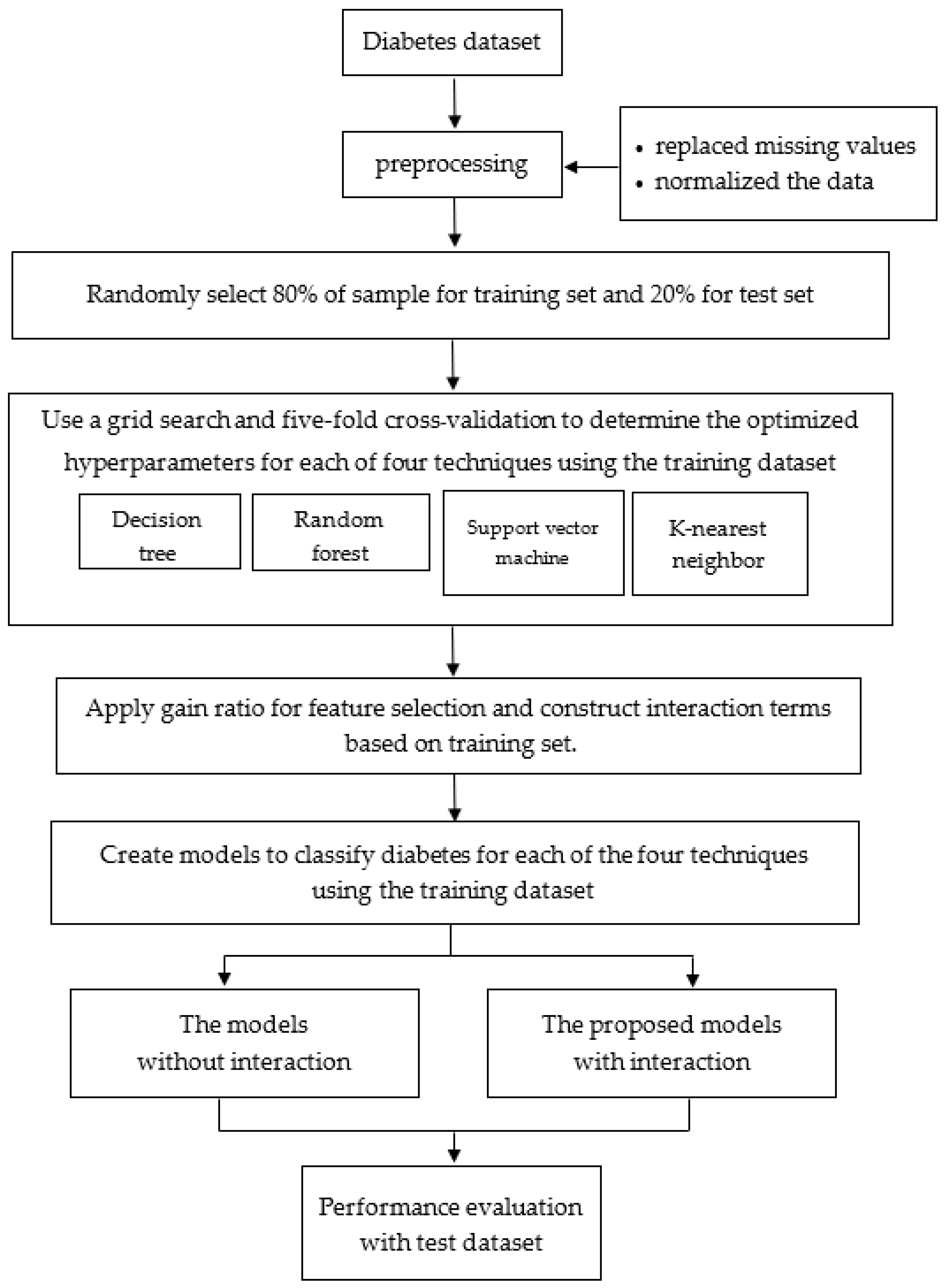
2. Materials and Methods

In this section, we propose the steps necessary to obtain new classification models with optimized hyperparameter values and interaction terms, as well as to compare the performance of the proposed classification models to models without interaction terms.
Step 1. After cleaning the data, 80% of the total 20,227 samples are randomly selected for data training and the remaining 20% are used for testing.
Step 2. Grid search and five-fold cross-validation are applied to the training dataset to determine the hyperparameters for the machine learning techniques.
Step 3. Feature selection using gain ratio is applied to construct the interaction terms based on the training dataset.
Step 4. The hyperparameters obtained from Step 2 are used to build the classification models without interaction terms and with interaction terms constructed in Step 3 using the training dataset.
Step 5. The four classification models are evaluated with and without interactions using the test dataset based on accuracy, precision, recall, and the F1-score calculated from the values in the confusion matrix as shown in Table 1 using Equations (1)–(4).
The flowchart of the process of creating classification models is shown in Figure 2.
Here, FP = false positive, FN = false negative, TN = true negative, and TP = true positive.
Accuracy = TP + TN TP + TN + FP + FN
Precision   = TP TP + FP
Recall   = TP TP + FN
F 1 score   = 2 × ( Precision   × Recall   Precision + Recall   )

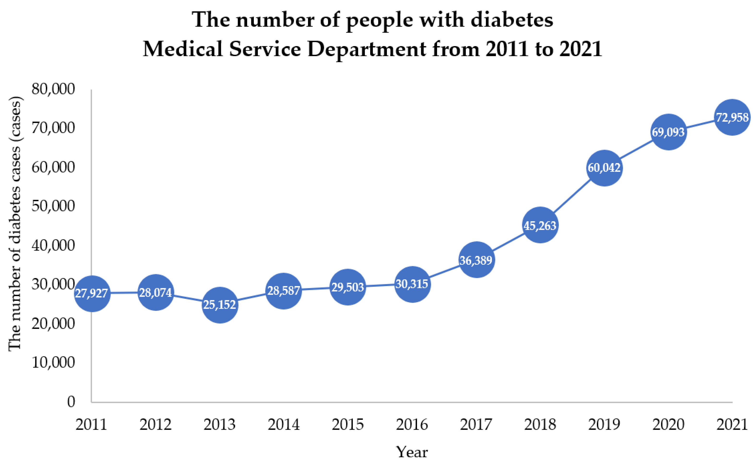
2.1. Data Collection

The diabetes dataset used in this study was obtained from the Department of Medical Services, Bangkok, between 2019 and 2021 and was desensitized.
The dataset consists of 20,227 records and 10 attributes related to diabetes risk. These attributes were not only selected by considering the diabetes risk assessment form created by the Diabetes Association of Thailand under the patronage of Her Royal Highness Princess Maha Chakri Sirindhorn, but also the completeness of hospital database. These 10 attributes are: sex; age; weight; height; body mass index (BMI); diastolic blood pressure (DIA); systolic blood pressure (SYS); resting heart rate (RHR); family history of diabetes; and diabetes diagnosis results. The outcome variable is the diabetes diagnosis result, which has two values: 0 for non-diabetes and 1 for diabetes (both Type 1 and Type 2). Those patients with diabetes were identified by their doctor according to a diagnostic code for diabetes (International Classification of Diseases: E10–E14) [10]. The description of the dataset and the results of the univariate data analysis for each group of the diabetes diagnosis result are shown in Table 2 and Table 3.

2.2. Data Preprocessing

Preprocessing helps transform data so that a better machine learning model can be built, thereby providing higher accuracy. In this study, we replaced missing values with the mean values of the available data.
To put all the variables on the same scale, we normalized the data to a range of 0–1 using Equation (5).
x * = X min ( x ) max ( x ) min ( x )
Here, x* = the normalized value, X = original value, min(x) = the lowest value of the dataset, and max(x) = the highest value of the dataset.

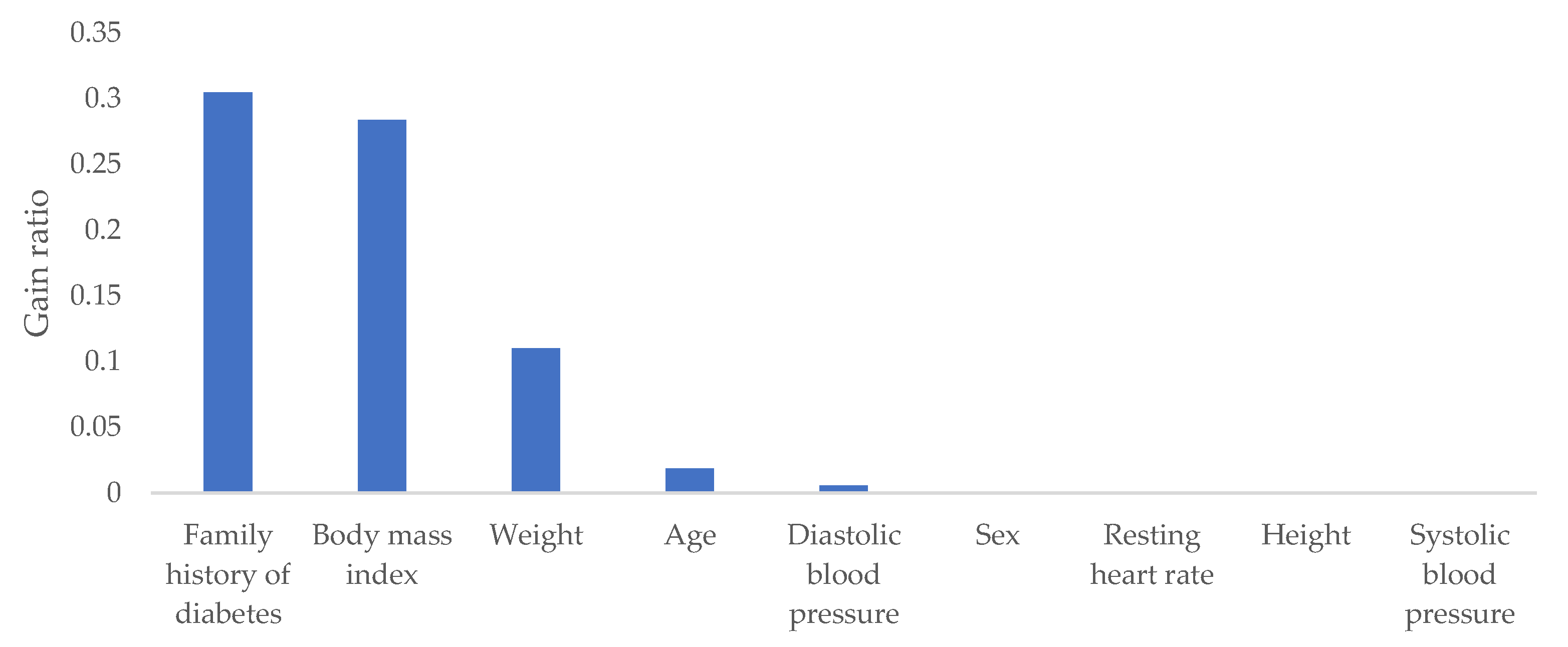
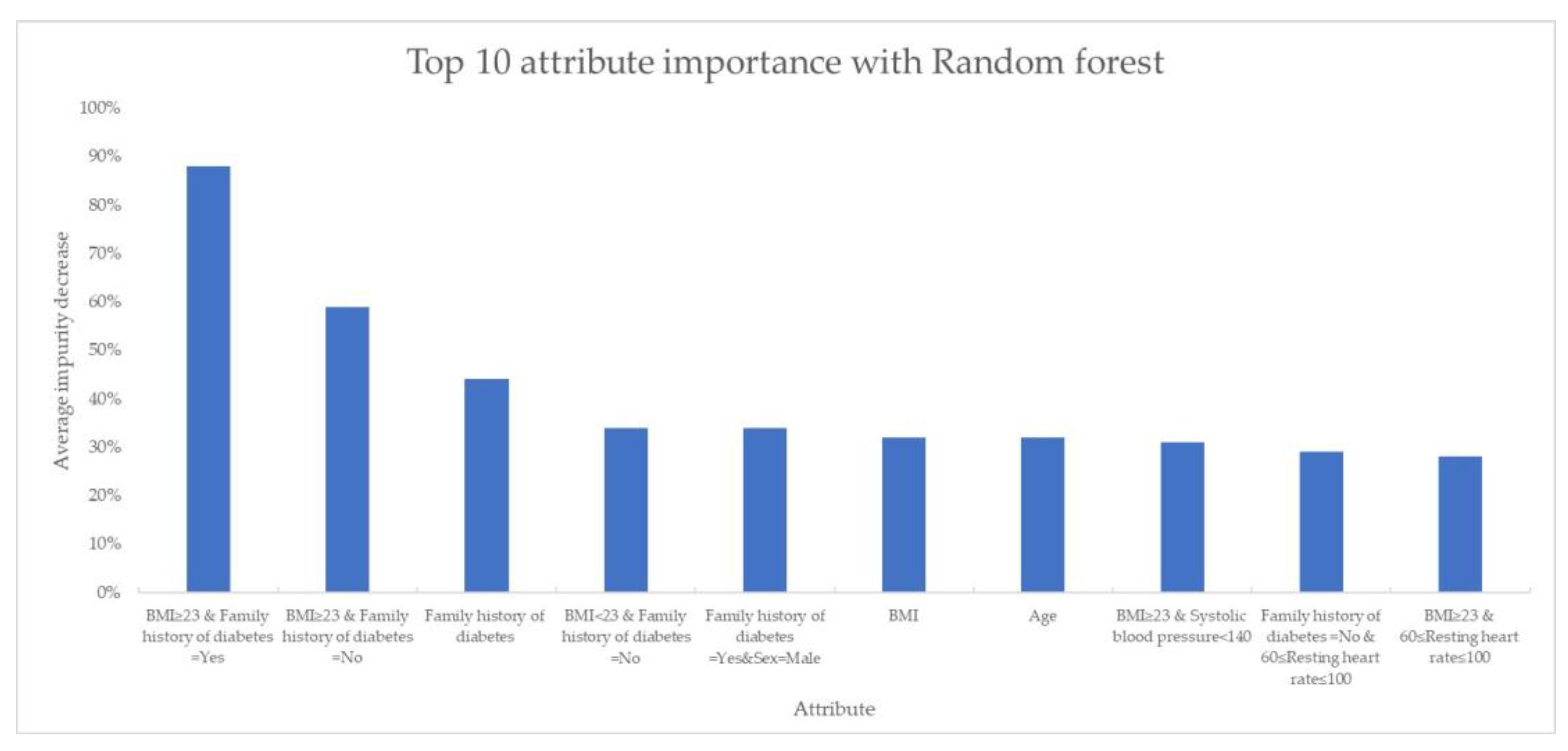
2.3. Feature Selection and Construction

Feature selection and construction is an important step in classification modeling. It could not only help increase the classification accuracy but also improve the efficiency of practical operations. In this study, we applied a feature selection technique (gain ratio) to rank the features based on their importance in the classification of diabetes. To calculate gain ratio, split information is required, which can be calculated as follows [11]
Information gain(S,a) = H(S) − H(S|a)
H ( S ) = j = 1 y P ( S ) log 2 P ( S )
H ( S | a ) = j = 1 y P ( S | a ) log 2 P ( S | a )
where Information gain(S,a) is the information for the dataset S for the attribute a, H(S) is the entropy for the dataset S, H(S|a) is the conditional entropy for the dataset S given the attribute a, P ( S ) is the probability of the dataset S, and P(S|a) is the conditional probability of the dataset S given the attribute a.
SplitInformation a ( S ) = j = 1 y S j S log 2 ( S j S )
where SplitInformation a ( S )   represents the amount of data considered by dividing the data in the dataset S into y subsets based on the values in attribute a, and S j being the number of times that j occurs divided by the total count of events S.
Next the gain ratio is calculated by
Gain   ratio ( S , a ) = Information   gain ( S , a ) SplitInformation a ( S )
where Gain ratio(S,a) represents the information gain achieved by dividing the dataset S into subsets based on the attribute a. The feature with maximum gain ratio is chosen as the best classification feature.
According to a relevant research study, classification models with interaction terms are shown to be more efficient than the models without interaction terms [12]. Based on the results from the gain ratio method, it was found that family history of diabetes and body mass index were the most important to predict diabetes, as shown in Figure 3. Therefore, in this study, we included the interactions of these two most important risk factors affecting diabetes and the other factors into the models as shown in Table 4 and Table 5.
In this study, we determine thresholds for feature interactions based on the following literature reviews. From the Kaiser Permanente Northern California Diabetes Registry, it was found that 96% of adults age ≥ 60 years had diabetes [13]. The U.S. Preventive Services Task Force (USPSTF) and the American Diabetes Association (ADA) recommend screening for diabetes and prediabetes based on a body mass index ≥ 23 kg/ m 2 [14].
We selected three attributes in the form of “If X i   =   x i and X j   =   x j , then Y   =   y ”, where x i is the level of attribute; X i , x j is the level of attribute X j ; and y is the level of response Y”. We generated the interactions between X i and X j by labeling each interaction as 1 if X i   =   x i and X j   =   x j and labeling each interaction as 0 otherwise. This interaction is denoted by X i ( x i ) X j ( x j ) . For example, according to “If X 1   =   0 and X 2   =   1 , then Y   =   1 ”, we created an interaction between X 1 and X 2 , denoted by X 1 ( 0 ) X 2 ( 1 ) . The level of Y does not play any role in generating the variables.

2.4. Classification Methods

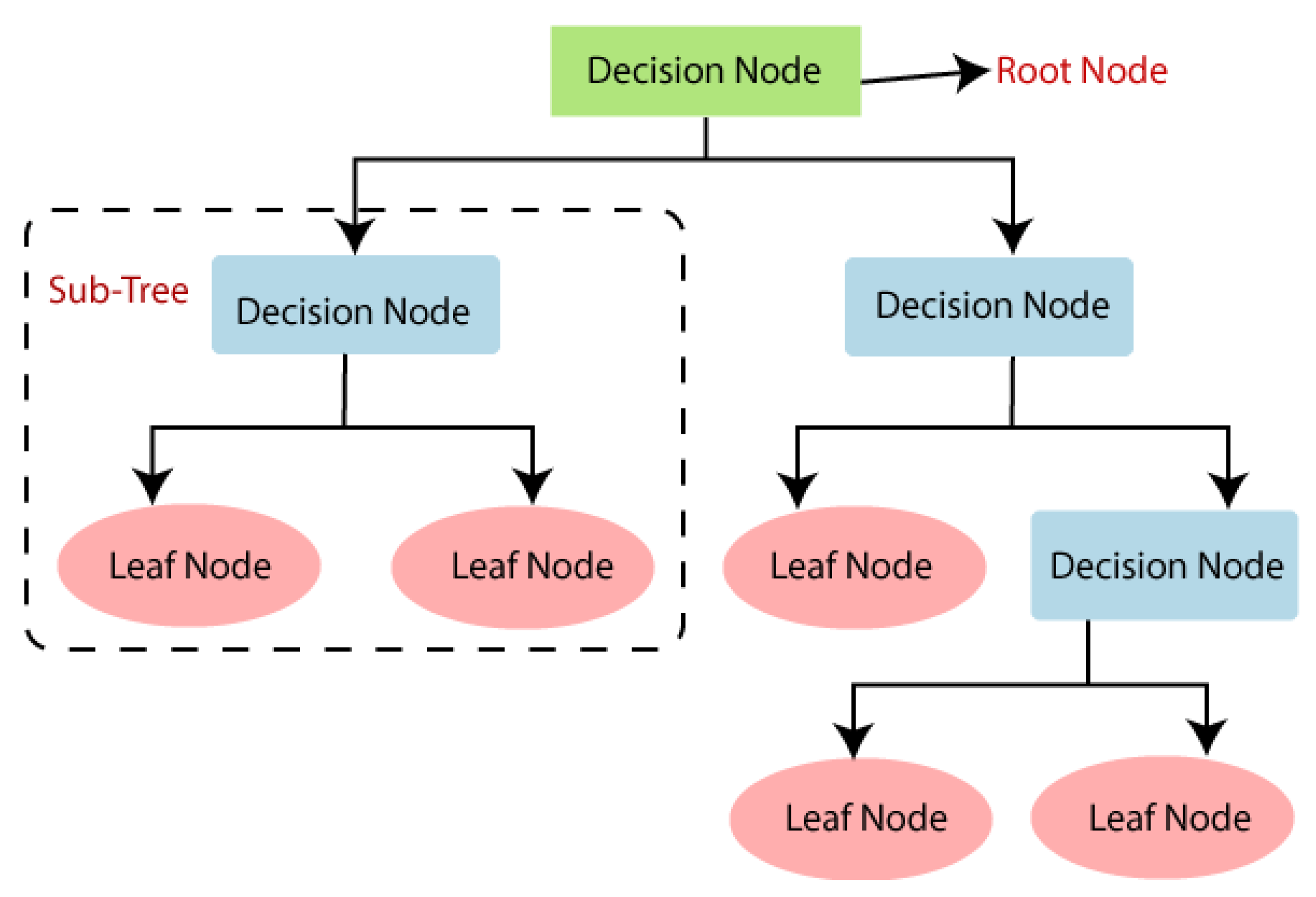
2.4.1. Decision Tree

Decision tree is a supervised machine learning algorithm used to solve classification problems. It uses decision nodes to classify the instances with different features [15]. A representation of a decision tree is shown in Figure 4.

2.4.2. Random Forest

The random forest classifier creates multiple decision trees by randomly selecting subsets of the training dataset. Then, it aggregates the votes from different decision trees to decide the final class of test objects [9]. The steps in which this occurs are given below [9].
Step 1. Random samples are selected from a given training dataset.
Step 2. This algorithm constructs a decision tree for all training data.
Step 3. Voting takes place by averaging the decision tree.
Step 4. Finally, the prediction result with the most votes is selected as the final prediction result.

2.4.3. Support Vector Machine

The concept of classification using the support vector machine algorithm is simply an attempt to find the best hyperplane that functions as a separator of two classes of data in the input space [17].

2.4.4. K-Nearest Neighbor

K-NN is a supervised algorithm applied to classify a set of data based on the nearest neighbors whose class is known. The steps for K-NN are given below [17]:
Step 1. Based on the definition of the K value, determine the optimum K value by finding the accuracy value in the training data using K-fold cross-validation.
Step 2. Calculate the distance between the test data and the training data using distance measures.
Step 3. Sort the results of the Euclidean distance calculation from the test data group in ascending order.
Step 4. Take K-nearest neighbors from the results that have been sorted for each set of test data. The test data class is taken from the majority vote among the K-nearest neighbors.

2.5. Software Tool

We used Weka, an open-source machine learning software tool used for diabetes classification analysis [18]. Weka contains algorithms for data processing, clustering, classification, regression, visualization, and feature selection. The algorithms used for classification via decision tree, support vector machine, and K-nearest neighbor are J48, SMO, and IBk, respectively.

3. Results

3.1. Hyperparameters for Machine Learning Techniques

In order to determine the hyperparameters for all machine learning techniques, we applied a grid search technique and five-fold cross-validation to the training dataset and compared the classification results based on accuracy, precision, recall, and the F1-score.

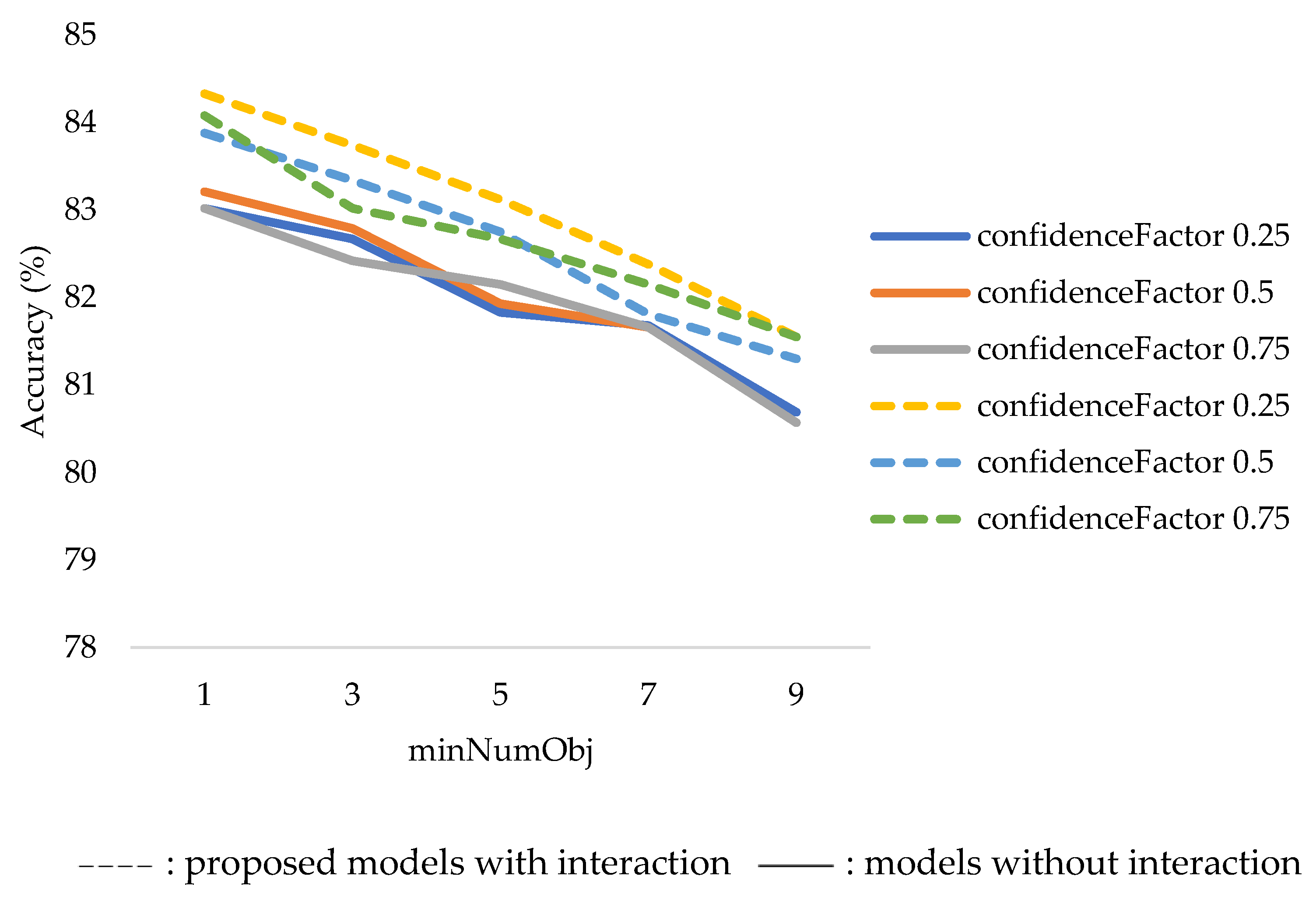
3.1.1. Decision Tree

The hyperparameters used in the decision tree are as follows:
  • ConfidenceFactor refers to the confidence intervals used in branching.
  • MinNumObj refers to the minimum amount of learned information in the leaf node.
The hyperparameters for the models with and without interaction terms are shown in Table 6.
Based on the result of five-fold cross-validation of the models without interaction, the hyperparameters that yielded the highest accuracy were confidenceFactor = 0.5 and minNumObj = 1, which provided an accuracy of 83.02%. Regarding the proposed models with interaction, the values were confidenceFactor = 0.25 and minNumObj = 1, which provided an accuracy of 84.08%, as shown in Figure 5.

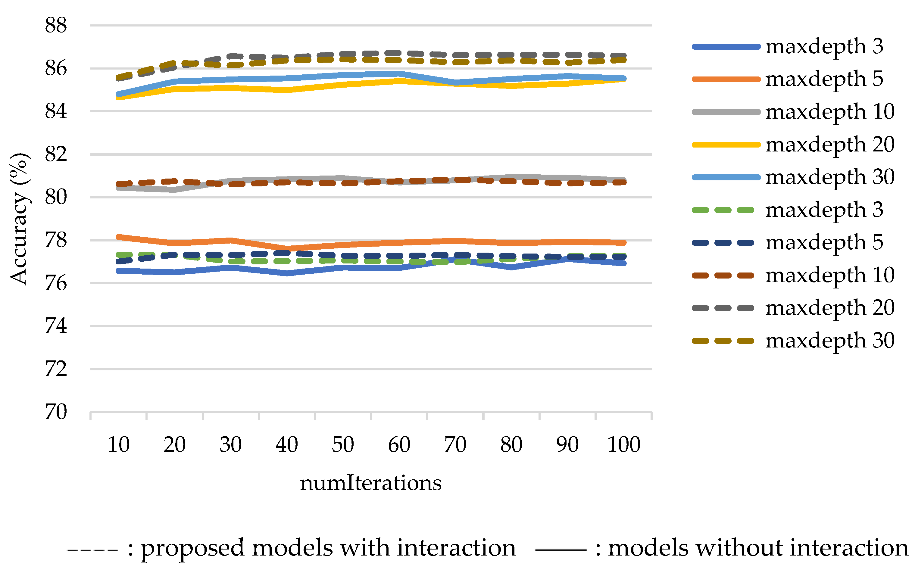
3.1.2. Random Forest

The hyperparameters used in the random forest are as follows:
  • NumIterations refers to the total number of trees to be built.
  • MaxDepth refers to the maximum depth of the trees.
The hyperparameters for the models with and without interaction are shown in Table 7.
Based on the results of the five-fold cross-validation of the models without interaction, the hyperparameters that yielded the highest accuracy were numIterations = 60 and maxDepth = 30, which provided an accuracy of 85.76%. Regarding the proposed models with interaction, the values were numIterations = 60 and maxDepth = 20, which provided an accuracy of 86.72%, as shown in Figure 6.

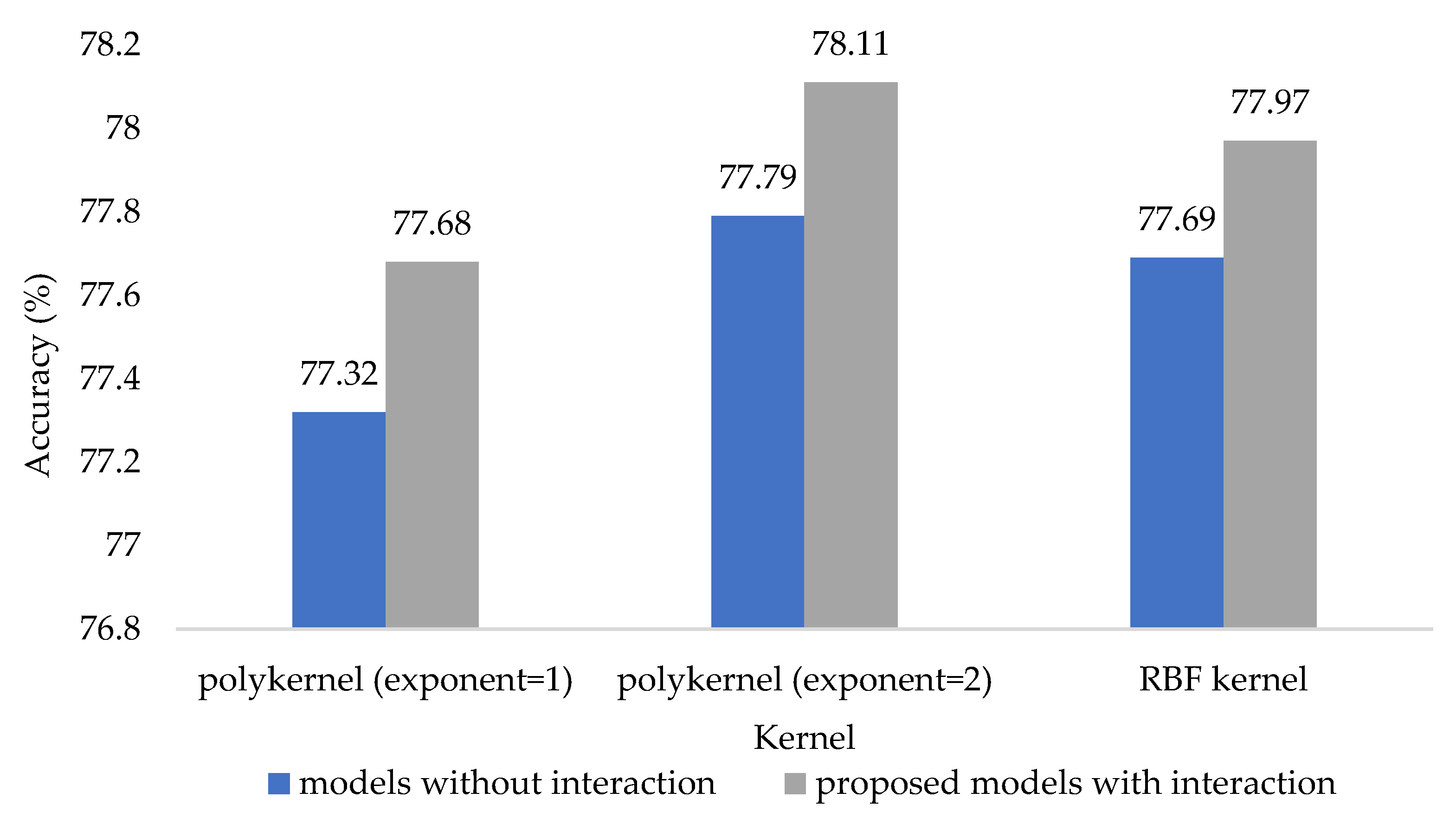
3.1.3. Support Vector Machine

The hyperparameters used in the support vector machine are as follows:
  • C refers to the regularization parameter.
  • Kernel refers to the different types of mathematical functions, such as linear, polynomial, and RBF (radial basis function).
  • Exponent refers to the exponent of the polykernel.
  • Gamma refers to the hyperparameter that influences the learning dataset of the RBF kernel.
The hyperparameters for the models with and without interaction terms are shown in Table 8.
According to the grid search, different kernels yield different optimal C values as follows:
  • kernel = polykernel (exponent = 1); C = 5.
  • kernel = polykernel (exponent = 2); C = 5.
  • kernel = RBF, C = 10, gamma = 0.1.
Based on the five-fold cross-validation results of the models with and without interaction terms, the hyperparameters that yield the highest accuracy were kernel = polykernel (exponent = 2) and C = 5. The case in which the proposed models with interaction terms provided an accuracy of 78.11% and the models without interaction terms provided an accuracy of 77.79% is shown in Figure 7.

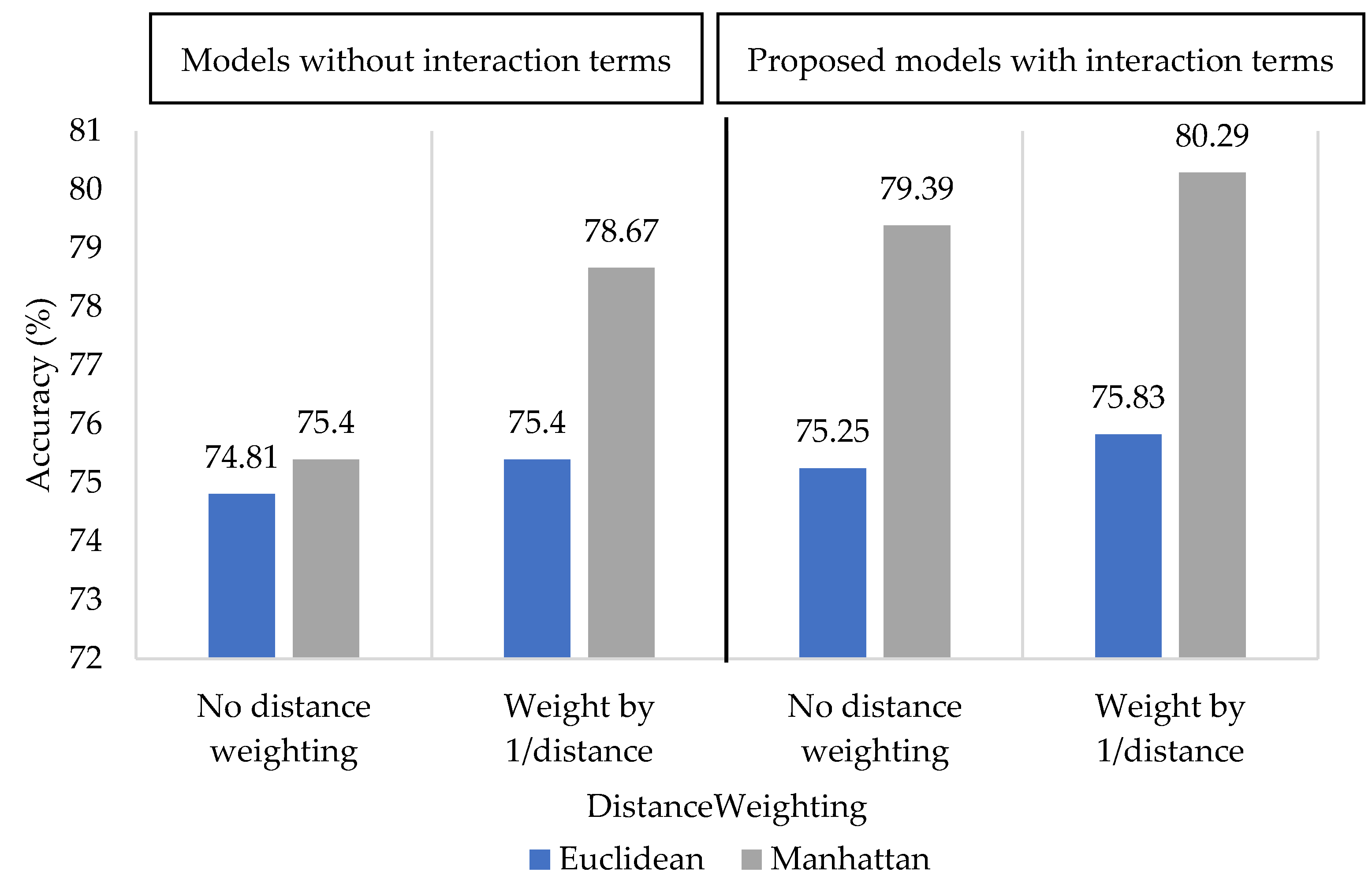
3.1.4. K-Nearest Neighbor

The hyperparameters used in K-nearest neighbor are as follows:
  • K refers to the number of neighbor points used.
  • distanceFunction refers to the distance function for finding neighbors. DistanceWeighting refers to the weighting function.
The hyperparameters for the models with and without interaction terms are shown in Table 9 and Figure 8.
According to the grid search, different distanceFunctions yield different optimal DistanceWeighting and K values, as follows:
The models without interaction terms:
  • distanceFunction = Euclidean, DistanceWeighting = Weight by 1/distance, K = 17.
  • distanceFunction = Manhattan, DistanceWeighting = Weight by 1/distance, K = 21.
The proposed models with interaction terms:
  • distanceFunction = Euclidean, DistanceWeighting = Weight by 1/distance, K = 11.
  • distanceFunction = Manhattan, DistanceWeighting = Weight by 1/distance, K = 13.
Based on the five-fold cross-validation results of the models without interaction terms, the hyperparameters that yielded the highest accuracy were distanceFunction = Manhattan, DistanceWeighting = Weight by 1/distance, and K = 21, which provided an accuracy of 80.49%. Regarding the proposed models with interaction terms, the values were distanceFunction = Manhattan, DistanceWeighting = Weight by 1/distance, and K = 13, which provided an accuracy of 81.12%, as shown in Figure 9.

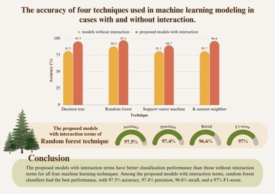
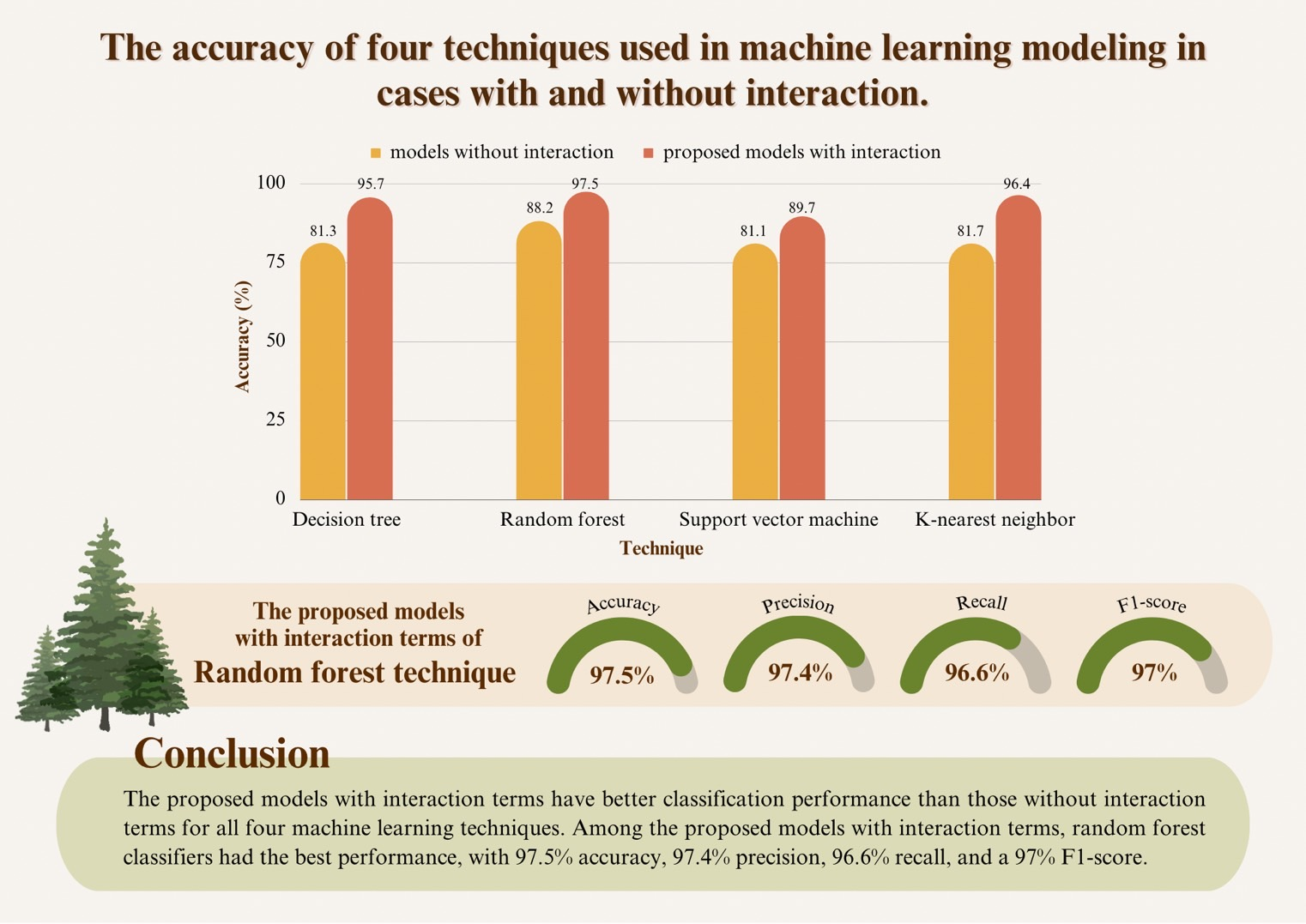
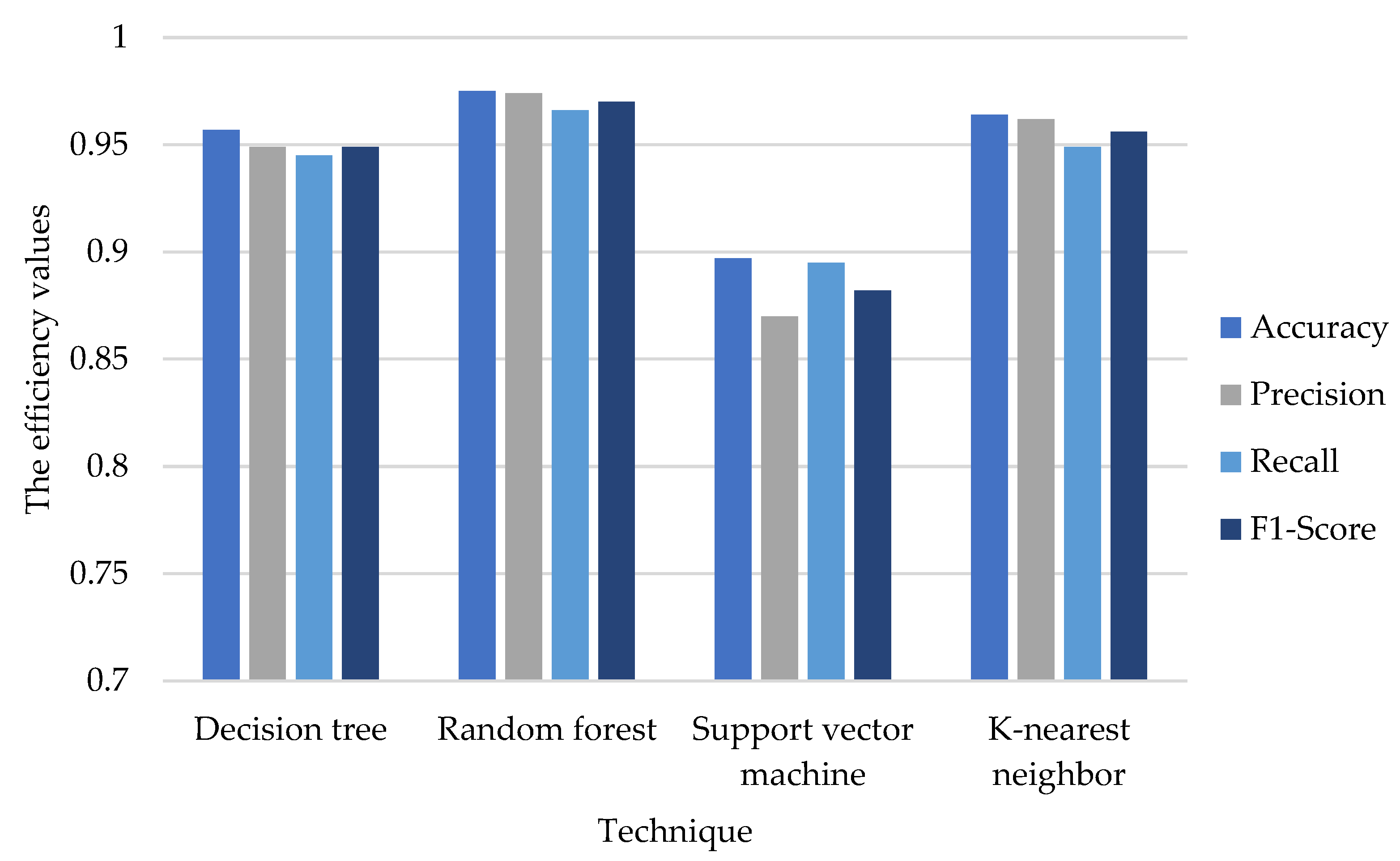
3.2. Comparison of the Efficiency of the Four Techniques

A comparison of the four techniques with and without interaction terms is shown in Table 10. The performance was based on accuracy, precision, recall, and the F1-score.
As shown in Table 10, the proposed models with interaction terms had better classification performance than those without interaction terms across all four techniques.
As shown in Figure 10, among the proposed models with interaction terms, random forest performed the best, with 97.5% accuracy, 97.4% precision, 96.6% recall, and a 97% F1-score. In addition, according to the t-test results in Table 11, the accuracy of the proposed model with interaction terms using random forest is significantly higher than that of the other three techniques at a significance level of 0.05. The top 10 attribute importance evaluation with random forest is shown in Figure 11.

4. Discussion and Conclusions

In conclusion, this research presents new classification models that incorporate optimized hyperparameters and include the interaction of important risk factors affecting diabetes. The results reveal that, upon tuning the hyperparameters and including the interaction terms, the proposed models have better performance than those without interaction terms for all four techniques (decision tree, random forest, support vector machine, and K-nearest neighbor). Among the proposed models with interaction terms, random forest had the best performance classification, with 97.5% accuracy, 97.4% precision, 96.6% recall, and a 97% F1-score.
The proposed models with interaction terms are more efficient than the models without interaction terms because we included interaction with important risk factors affecting diabetes, body mass index, and a family history of diabetes in the models. The findings from this research can be further developed into a program to effectively screen potential diabetes patients in the future.
Nevertheless, other attributes related to exercise, lifestyle (such as waist-to-height ratio), and dietary management (including protein, fat, and sugar intake control) have also been identified as important risk factors for diabetes [19]. Moreover, certain metabolites have been associated with prediabetes and diabetes [20]. Therefore, future research may consider including these risk factors into consideration when creating classification models for diabetes.

Author Contributions

Conceptualization, M.P. and S.H.; methodology, M.P.; software, M.P.; validation, S.H.; formal analysis, M.P.; investigation, M.P.; resources, S.H.; data curation, M.P.; writing—original draft preparation, M.P. and S.H.; writing—review and editing, M.P. and S.H.; visualization, M.P.; supervision, S.H.; project administration, S.H.; funding acquisition, S.H. All authors have read and agreed to the published version of the manuscript.

Funding

This research was funded by Faculty of Science, Silpakorn University grant number SRIF-JRG-2566-06 and The APC was funded by Silpakorn University Research, Innovation and Creativity Administration Office (SURIC).

Institutional Review Board Statement

The study was conducted in accordance with the Declaration of Helsinki, and approved by the Institutional Review Board (or Ethics Committee) of Bangkok Metropolitan Administration Human Research Ethics Committee (protocol code U005hh/66_EXP and date of approval 22 March 2023).

Informed Consent Statement

Not applicable.

Data Availability Statement

Restrictions apply to the availability of these data. Data was obtained from the Medical Service Department of Bangkok, Thailandand are available from the authors with the permission of the Medical Service Department of Bangkok, Thailand.

Conflicts of Interest

The authors declare no conflict of interest.

Correction Statement

This article has been republished with a minor correction to Equation (7). This change does not affect the scientific content of the article.

References

  1. Available online: https://www.who.int/news-room/fact-sheets/detail/diabetes (accessed on 29 April 2023).
  2. Available online: https://www.cdc.gov/diabetes/library/spotlights/diabetes-facts-stats.html (accessed on 29 April 2023).
  3. Griffin, P.; Rodgers, M.D. Type 1 Diabetes. National Institute of Diabetes and Digestive and Kidney Diseases. Available online: https://www.niddk.nih.gov/health-information/diabetes/overview/what-is-diabetes/type-1-diabetes (accessed on 14 April 2023).
  4. Griffin, P.; Rodgers, M.D. Risk Factors for Type 2 Diabetes. National Institute of Diabetes and Digestive and Kidney Diseases. Available online: https://www.niddk.nih.gov/health-information/diabetes/overview/risk-factors-type-2-diabetes (accessed on 14 April 2023).
  5. Available online: https://www.cdc.gov/diabetes/basics/risk-factors.html (accessed on 29 April 2023).
  6. Pacharawongsakda, E. An Introduction to Data Mining Techniques; Pearson Education: London, UK, 2014. [Google Scholar]
  7. Wei, S.; Zhao, X.; Miao, C. A comprehensive exploration to the machine learning techniques for diabetes identification. In Proceedings of the 2018 IEEE 4th World Forum on Internet of Things (WF-IoT), Singapore, 5–8 February 2018; pp. 291–295. [Google Scholar] [CrossRef]
  8. Zou, Q.; Qu, K.; Luo, Y.; Yin, D.; Ju, Y.; Tang, H. Predicting Diabetes Mellitus with Machine Learning Techniques. Front Genet. 2018, 9, 515. [Google Scholar] [CrossRef] [PubMed]
  9. Sneha, N.; Tarun, G. Analysis of diabetes mellitus for early prediction using optimal features selection. J. Big Data 2019, 6, 13. [Google Scholar] [CrossRef]
  10. International Statistical Classification of Diseases and Related Health Problems 10th Revision. Available online: https://icd.who.int/browse10/2019/en#/E10-E14 (accessed on 29 April 2023).
  11. Available online: https://en.wikipedia.org/wiki/Information_gain_ratio#References (accessed on 29 April 2023).
  12. Changpetch, P.; Pitpeng, A.; Hiriote, S.; Yuangyai, C. Integrating Data Mining Techniques for Naïve Bayes Classification: Applications to Medical Datasets. Computation 2021, 9, 99. [Google Scholar] [CrossRef]
  13. Laiteerapong, N.; Karter, A.J.; Liu, J.Y.; Moffet, H.H.; Sudore, R.; Schillinger, D.; John, P.M.; Huang, E.S. Correlates of quality of life in older adults with diabetes: The Diabetes & Aging Study. Diabetes Care 2011, 34, 1749–1753. [Google Scholar] [CrossRef] [PubMed] [Green Version]
  14. Davidson, K.W.; Barry, M.J.; Mangione, C.M.; Cabana, M.; Caughey, A.B.; Davis, E.M.; Donahue, K.E.; Doubeni, C.A.; Krist, A.H.; Kubik, M.; et al. Screening for Prediabetes and Type 2 Diabetes: US Preventive Services Task Force Recommendation Stateme. JAMA 2021, 326, 736–743. [Google Scholar] [CrossRef] [PubMed]
  15. Deepti, S.; Dilip, S.S. Prediction of Diabetes using Classification Algorithms. In Proceedings of the International Conference on Computational Intelligence and Data Science (ICCIDS 2018), Gurugram, India, 7–8 April 2018; pp. 1578–1585. [Google Scholar] [CrossRef]
  16. Hafeez, M.A.; Rashid, M.; Tariq, H.; Abideen, Z.U.; Alotaibi, S.S.; Sinky, M.H. Performance Improvement of Decision Tree: A Robust Classifier Using Tabu Search Algorithm. Appl. Sci. 2021, 11, 6728. [Google Scholar] [CrossRef]
  17. Dimas, A.A.; Naqshauliza, D.K. Comparison of Accuracy Level of Support Vector Machine (SVM) and K-Nearest Neighbors (KNN) Algorithms in Predicting Heart Disease. Int. J. Emerg. Trends Eng. Res. 2020, 8, 1689–1694. [Google Scholar]
  18. Maneerat, P. WEKA Data Mining Program. 2012. Available online: https://maneerat-paranan.blogspot.com/2012/02/weka.html (accessed on 14 April 2023).
  19. Yang, H.; Luo, Y.; Ren, X.; Wu, M.; He, X.; Peng, B.; Deng, K. Risk Prediction of Diabetes: Big data mining with fusion of multifarious physical examination indicators. Inf. Fusion 2021, 75, 140–149. [Google Scholar] [CrossRef]
  20. Guasch-Ferre, M.; Hruby, A.; Toledo, E.; Clish, C.B.; Martínez-González, M.A.; Salas-Salvado, J.; Hu, F.B. Metabolomics in Prediabetes and Diabetes: A Systematic Review and Meta-analysis. Diabetes Care 2016, 39, 833–846. [Google Scholar] [CrossRef] [PubMed] [Green Version]
Figure 1. The number of diabetes cases in government hospitals in Bangkok under the Medical Service Department of Bangkok, Thailand, from 2011 to 2021.
Computation 11 00096 g001
Figure 2. The process of creating and comparing classification models.
Computation 11 00096 g002
Figure 3. A graphic to show the feature selection using gain ratio.
Computation 11 00096 g003
Figure 4. The model of the decision tree (Hafeez, 2021 [16]).
Computation 11 00096 g004
Figure 5. The accuracy of the models with and without interaction versus the hyperparameters of the decision tree.
Computation 11 00096 g005
Figure 6. The accuracy of the models with and without interaction terms versus the hyperparameters of the random forest model.
Computation 11 00096 g006
Figure 7. The accuracy of the models with and without interaction terms versus the hyperparameters of the support vector machine.
Computation 11 00096 g007
Figure 8. The accuracy of the models with and without interaction terms versus the hyperparameters of K-nearest neighbor.
Computation 11 00096 g008
Figure 9. The accuracy of the models with and without interaction terms versus K values when distanceFunction = Manhattan and DistanceWeighting = Weight by 1/distance.
Computation 11 00096 g009
Figure 10. Classification results for the proposed models with interaction terms.
Computation 11 00096 g010
Figure 11. The top 10 attribute importance evaluation with random forest.
Computation 11 00096 g011
Table 1. The confusion matrix.
Predicted
NoYes
ActualNo
Yes
TN
FN
FP
TP
Table 2. The attributes of the diabetes dataset.
AttributeMeasure
Diabetes diagnosis results0 = non-diabetes
1 = diabetes
Sex0 = male
1 = female
Ageyear
Weightkg
Heightcm.
Body mass indexkg/ m 2
Diastolic blood pressuremmHg
Systolic blood pressuremmHg
Resting heart ratebpm
Family history of diabetes0 = no
1 = yes
Table 3. The results of the univariate data analysis based on the diagnosis of diabetes.
AttributeDiabetesNon-Diabetes
Mean ± S.D.MinMaxMean ± S.D.MinMax
Age64 ± 10.96319462 ± 12.333197
Weight67 ± 14.713116762 ± 13.6930167
Height159 ± 8.46136195158 ± 8.49100195
Body mass index26.16 ± 4.9712.6645.7924.69 ± 4.7512.4945.18
Diastolic blood
pressure
71.83 ± 12.493515073.90 ± 11.8637128
Systolic blood
pressure
135.56 ± 18.3380237132.51 ± 17.7077198
Resting heart rate83.20 ± 14.093615182.43 ± 13.5936161
Table 4. Determination of attributes used to create interactions.
AttributeDetails
Sex
( X 1 )
X 1 = 0 if sex = male
X 1 = 1 if sex = female
Age
( X 2 )
X 2 = 0 if age < 60
X 2 = 1 if age ≥ 60
Body mass index
( X 3 )
X 3 = 0 if body mass index < 23
X 3 = 1 if body mass index ≥ 23
Diastolic blood pressure
( X 4 )
X 4 = 0 if diastolic blood pressure < 90
X 4 = 1 if diastolic blood pressure ≥ 90
Systolic blood pressure
( X 5 )
X 5 = 0 if systolic blood pressure < 140
X 5 = 1 if systolic blood pressure ≥ 140
Resting heart rate
( X 6 )
X 6 = 0 if 60 ≤ resting heart rate ≤ 100
X 6 = 1 if resting heart rate < 140 or resting heart rate > 100
Family history of diabetes
( X 7 )
X 7 = 0 if family history of diabetes = no
X 7 = 1 if family history of diabetes = yes
Table 5. The attributes of interaction variables.
Interaction VariableGenerated Interactions
X 3 = 0 and X 1 = 0 , then Y = 1 X 3 ( 0 ) X 1 ( 0 ) = 1 if X 3 = 0 and X 1   = 0
X 3 ( 0 ) X 1 ( 0 ) = 0 , otherwise
X 3 = 0 and X 1 = 1 , then Y = 1 X 3 ( 0 ) X 1 ( 1 ) = 1 if X 3 = 0 and X 1   = 1
X 3 ( 0 ) X 1 ( 1 ) = 0 , otherwise
X 3 = 1 and X 1 = 0 , then Y = 1 X 3 ( 1 ) X 1 ( 0 ) = 1 if X 3 = 1 and X 1   = 0
X 3 ( 1 ) X 1 ( 0 ) = 0 , otherwise
X 3 = 1 and X 1 = 1 , then Y = 1 X 3 ( 1 ) X 1 ( 1 ) = 1 if X 3 = 1 and X 1   = 1
X 3 ( 1 ) X 2 ( 1 ) = 0 , otherwise
X 3 = 0 and X 2 = 0 , then Y = 1 X 3 ( 0 ) X 2 ( 0 ) = 1 if X 3 = 0 and X 2   = 0
X 3 ( 0 ) X 2 ( 0 ) = 0 , otherwise
X 3 = 0 and X 2 = 1 , then Y = 1 X 3 ( 0 ) X 2 ( 1 ) = 1 if X 3 = 0 and X 2   = 1
X 3 ( 0 ) X 2 ( 1 ) = 0 , otherwise
X 3 = 1 and X 2 = 0 , then Y = 1 X 3 ( 1 ) X 2 ( 0 ) = 1 if X 3 = 1 and X 2   = 0
X 3 ( 1 ) X 2 ( 0 ) = 0 , otherwise
X 3 = 1 and X 2 = 1 , then Y = 1 X 3 ( 1 ) X 2 ( 1 ) = 1 if X 3 = 1 and X 2   = 1
X 3 ( 1 ) X 2 ( 1 ) = 0 , otherwise
X 3 = 0 and X 4 = 0 , then Y = 1 X 3 ( 0 ) X 4 ( 0 ) = 1 if X 3 = 0 and X 4   = 0
X 3 ( 0 ) X 4 ( 0 ) = 0 , otherwise
X 3 = 0 and X 4 = 1 , then Y = 1 X 3 ( 0 ) X 4 ( 1 ) = 1 if X 3 = 0 and X 4   = 1
X 3 ( 0 ) X 4 ( 1 ) = 0 , otherwise
X 3 = 1 and X 4 = 0 , then Y = 1 X 3 ( 1 ) X 4 ( 0 ) = 1 if X 3 = 1 and X 4   = 0
X 3 ( 1 ) X 4 ( 0 ) = 0 , otherwise
X 3 = 1 and X 4 = 1 , then Y = 1 X 3 ( 1 ) X 4 ( 1 ) = 1 if X 3 = 1 and X 4   = 1
X 3 ( 1 ) X 4 ( 1 ) = 0 , otherwise
X 3 = 0 and X 5 = 0 , then Y = 1 X 3 ( 0 ) X 5 ( 0 ) = 1 if X 3 = 0 and X 5   = 0
X 3 ( 0 ) X 5 ( 0 ) = 0 , otherwise
X 3 = 0 and X 5 = 1 , then Y = 1 X 3 ( 0 ) X 5 ( 1 ) = 1 if X 3 = 0 and X 5   = 1
X 3 ( 0 ) X 5 ( 1 ) = 0 , otherwise
X 3 = 1 and X 5 = 0 , then Y = 1 X 3 ( 1 ) X 5 ( 0 ) = 1 if X 3 = 1 and X 5   = 0
X 3 ( 1 ) X 5 ( 0 ) = 0 , otherwise
X 3 = 1 and X 5 = 1 , then Y = 1 X 3 ( 1 ) X 5 ( 1 ) = 1 if X 3 = 1 and X 5   = 1
X 3 ( 1 ) X 5 ( 1 ) = 0 , otherwise
X 3 = 0 and X 6 = 0 , then Y = 1 X 3 ( 0 ) X 6 ( 0 ) = 1 if X 3 = 0 and X 6   = 0
X 3 ( 0 ) X 6 ( 0 ) = 0 , otherwise
X 3 = 0 and X 6 = 1 , then Y = 1 X 3 ( 0 ) X 6 ( 1 ) = 1 if X 3 = 0 and X 6 = 1
X 3 ( 0 ) X 6 ( 1 ) = 0 , otherwise
X 3 = 1 and X 6 = 0 , then Y = 1 X 3 ( 1 ) X 6 ( 0 ) = 1 if X 3 = 1 and X 6   = 0
X 3 ( 1 ) X 6 ( 0 ) = 0 , otherwise
X 3 = 1 and X 6 = 1 , then Y = 1 X 3 ( 1 ) X 6 ( 1 ) = 1 if X 3 = 1 and X 6   = 1
X 3 ( 1 ) X 6 ( 1 ) = 0 , otherwise
X 3 = 0 and X 7 = 0 , then Y = 1 X 3 ( 0 ) X 7 ( 0 ) = 1 if X 3 = 0 and X 7   = 0
X 3 ( 0 ) X 7 ( 0 ) = 0 , otherwise
X 3 = 0 and X 7 = 1 , then Y = 1 X 3 ( 0 ) X 7 ( 1 ) = 1 if X 3 = 0 and X 7   = 1
X 3 ( 0 ) X 7 ( 1 ) = 0 , otherwise
X 3 = 1 and X 7 = 0 , then Y = 1 X 3 ( 1 ) X 7 ( 0 ) = 1 if X 3 = 1 and X 7   = 0
X 3 ( 1 ) X 7 ( 0 ) = 0 , otherwise
X 3 = 1 and X 7 = 1 , then Y = 1 X 3 ( 1 ) X 7 ( 1 ) = 1 if X 3 = 1 and X 7 = 1
X 3 ( 1 ) X 7 ( 1 ) = 0 , otherwise
X 7 = 0 and X 1 = 0 , then Y = 1 X 7 ( 0 ) X 1 ( 0 ) = 1 if X 7 = 0 and X 1 = 0
X 7 ( 0 ) X 1 ( 0 ) = 0 , otherwise
X 7 = 0 and X 1 = 1 , then Y = 1 X 7 ( 0 ) X 1 ( 1 ) = 1 if X 7 = 0 and X 1   = 1
X 7 ( 0 ) X 1 ( 1 ) = 0 , otherwise
X 7 = 1 and X 1 = 0 , then Y = 1 X 7 ( 1 ) X 1 ( 0 ) = 1 if X 7 = 1 and X 1   = 0
X 7 ( 1 ) X 1 ( 0 ) = 0 , otherwise
X 7 = 1 and X 1 = 1 , then Y = 1 X 7 ( 1 ) X 1 ( 1 ) = 1 if X 7 = 1 and X 1   = 1
X 7 ( 1 ) X 2 ( 1 ) = 0 , otherwise
X 7 = 0 and X 2 = 0 , then Y = 1 X 7 ( 0 ) X 2 ( 0 ) = 1 if X 7 = 0 and X 2   = 0
X 7 ( 0 ) X 2 ( 0 ) = 0 , otherwise
X 7 = 0 and X 2 = 1 , then Y = 1 X 7 ( 0 ) X 2 ( 1 ) = 1 if X 7 = 0 and X 2 = 1
X 7 ( 0 ) X 2 ( 1 ) = 0 , otherwise
X 7 = 1 and X 2 = 0 , then Y = 1 X 7 ( 1 ) X 2 ( 0 ) = 1 if X 7 = 1 and X 2 = 0
X 7 ( 1 ) X 2 ( 0 ) = 0 , otherwise
X 7 = 1 and X 2 = 1 , then Y = 1 X 7 ( 1 ) X 2 ( 1 ) = 1 if X 7 = 1 and X 2   = 1
X 7 ( 1 ) X 2 ( 1 ) = 0 , otherwise
X 7 = 0 and X 4 = 0 , then Y = 1 X 7 ( 0 ) X 4 ( 0 ) = 1 if X 7 = 0 and X 4   = 0
X 7 ( 0 ) X 4 ( 0 ) = 0 , otherwise
X 7 = 0 and X 4 = 1 , then Y = 1 X 7 ( 0 ) X 4 ( 1 ) = 1 if X 7 = 0 and X 4   = 1
X 7 ( 0 ) X 4 ( 1 ) = 0 , otherwise
X 7 = 1 and X 4 = 0 , then Y = 1 X 7 ( 1 ) X 4 ( 0 ) = 1 if X 7 = 1 and X 4   = 0
X 7 ( 1 ) X 4 ( 0 ) = 0 , otherwise
X 7 = 1 and X 4 = 1 , then Y = 1 X 7 ( 1 ) X 4 ( 1 ) = 1 if X 7 = 1 and X 4   = 1
X 7 ( 1 ) X 4 ( 1 ) = 0 , otherwise
X 7 = 0 and X 5 = 0 , then Y = 1 X 7 ( 0 ) X 5 ( 0 ) = 1 if X 7 = 0 and X 5   = 0
X 7 ( 0 ) X 5 ( 0 ) = 0 , otherwise
X 7 = 0 and X 5 = 1 , then Y = 1 X 7 ( 0 ) X 5 ( 1 ) = 1 if X 7 = 0 and X 5   = 1
X 7 ( 0 ) X 5 ( 1 ) = 0 , otherwise
X 7 = 1 and X 5 = 0 , then Y = 1 X 7 ( 1 ) X 5 ( 0 ) = 1 if X 7 = 1 and X 5   = 0
X 7 ( 1 ) X 5 ( 0 ) = 0 , otherwise
X 7 = 1 and X 5 = 1 , then Y = 1 X 7 ( 1 ) X 5 ( 1 ) = 1 if X 7 = 1 and X 5   = 1
X 7 ( 1 ) X 5 ( 1 ) = 0 , otherwise
X 7 = 0 and X 6 = 0 , then Y = 1 X 7 ( 0 ) X 6 ( 0 ) = 1 if X 7 = 0 and X 6   = 0
X 7 ( 0 ) X 6 ( 0 ) = 0 , otherwise
X 7 = 0 and X 6 = 1 , then Y = 1 X 7 ( 0 ) X 6 ( 1 ) = 1 if X 7 = 0 and X 6   = 1
X 7 ( 0 ) X 6 ( 1 ) = 0 , otherwise
X 7 = 1 and X 6 = 0 , then Y = 1 X 7 ( 1 ) X 6 ( 0 ) = 1 if X 7 = 1 and X 6   = 0
X 7 ( 1 ) X 6 ( 0 ) = 0 , otherwise
X 7 = 1 and X 6 = 1 , then Y = 1 X 7 ( 1 ) X 6 ( 1 ) = 1 if X 7 = 1 and X 6   = 1
X 7 ( 1 ) X 6 ( 1 ) = 0 , otherwise
Table 6. The hyperparameters for the decision tree model.
HyperparameterHyperparameter Value
confidenceFactor0.25, 0.5, 0.75
minNumObj1, 3, 5, 7, 9
Table 7. The hyperparameters for the random forest model.
HyperparameterHyperparameter Value
numIterations10, 20, ..., 100
maxDepth3, 5, 10, 20, none
Table 8. The hyperparameters for the support vector machine model.
HyperparameterHyperparameter Value
C5, 10, 15, ..., 50
kernelpolykernel (exponent = 1),
polykernel (exponent = 2, …, 5),
RBF
exponent2, 3, 4, 5
gamma0.05, 0.1, 0.2, 0.5, 1
Table 9. The hyperparameters for the K-nearest neighbor model.
HyperparameterHyperparameter Value
K1, 3, ..., 31
distanceFunctionEuclidean, Manhattan
DistanceWeightingNo distance weighting,
Weight by 1/distance
Table 10. The efficiency of the four techniques used in machine learning modeling for diabetic classification in cases with and without interaction terms.
ModelTechniqueAccuracyPrecisionRecallF1-Score
The models without interaction termsDecision tree0.8130.7970.7770.783
Random forest0.8820.9220.8930.907
Support vector machine0.8110.7640.7740.769
K-nearest neighbor0.8170.7840.7810.787
The proposed models with interaction termsDecision tree0.9570.9490.9450.949
Random forest0.9750.9740.9660.970
Support vector machine0.8970.8700.8950.882
K-nearest neighbor0.9640.9620.9490.956
Table 11. Performance testing of the diabetes classification models with interaction terms.
HypothesestSig.
H 0 : No difference in accuracy b/w random forest and decision tree.
H 1 : Random forest has more accuracy than decision tree.
−14.7970.001 *
H 0 : No difference in accuracy b/w random forest and support vector machine.
H 1 : Random forest has more accuracy than support vector machine.
−11.9110.001 *
H 0 : No difference in accuracy b/w random forest and K-nearest neighbor.
H 1 : Random forest has more accuracy than K-nearest neighbor.
−10.2050.02 *
* A statistically significant test result at 0.05 level.
Disclaimer/Publisher’s Note: The statements, opinions and data contained in all publications are solely those of the individual author(s) and contributor(s) and not of MDPI and/or the editor(s). MDPI and/or the editor(s) disclaim responsibility for any injury to people or property resulting from any ideas, methods, instructions or products referred to in the content.

