Article

A Two-Step Machine Learning Method for Predicting the Formation Energy of Ternary Compounds

1
Dynamics of Condensed Matter, Chair of Theoretical Chemistry, University of Paderborn, Warburger Str. 100, 33098 Paderborn, Germany
2
Department of Mathematics, Humboldt-Universität zu Berlin, Unter den Linden 6, 10099 Berlin, Germany
3
Department of Computer Science, University of Paderborn, Warburger Str. 100, 33098 Paderborn, Germany
4
Paderborn Center for Parallel Computing (PC2), University of Paderborn, Warburger Str. 100, 33098 Paderborn, Germany
5
Center for Sustainable Systems Design, University of Paderborn, Warburger Str. 100, 33098 Paderborn, Germany
*
Author to whom correspondence should be addressed.
Computation 2023, 11(5), 95; https://doi.org/10.3390/computation11050095
Submission received: 27 March 2023 / Revised: 24 April 2023 / Accepted: 5 May 2023 / Published: 9 May 2023
(This article belongs to the Section Computational Chemistry)

Abstract

:
Predicting the chemical stability of yet-to-be-discovered materials is an important aspect of the discovery and development of virtual materials. The conventional approach for computing the enthalpy of formation based on ab initio methods is time consuming and computationally demanding. In this regard, alternative machine learning approaches are proposed to predict the formation energies of different classes of materials with decent accuracy. In this paper, one such machine learning approach, a novel two-step method that predicts the formation energy of ternary compounds, is presented. In the first step, with a classifier, we determine the accuracy of heuristically calculated formation energies in order to increase the size of the training dataset for the second step. The second step is a regression model that predicts the formation energy of the ternary compounds. The first step leads to at least a 100% increase in the size of the dataset with respect to the data available in the Materials Project database. The results from the regression model match those from the existing state-of-the-art prediction models. In addition, we propose a slightly modified version of the Adam optimizer, namely centered Adam, and report the results from testing the centered Adam optimizer.

1. Introduction

A key step in the data-driven materials discovery process is predicting the enthalpy of formation (the formation energy) for compounds that have not been synthesized yet [1]. Knowledge about the formation energy of a compound helps determine whether the compound is thermodynamically stable against competing phases. The phase stability can be determined using convex hull analysis [2]. In a compositional phase diagram, a convex hull is constructed by connecting the lowest formation energies. Compounds that lie on the convex hull are thermodynamically stable, and the ones above the hull are metastable or unstable [3]. In this regard, the computing of formation energies has an important role in virtual materials discovery. The formation energy of a compound can be calculated using an existing and popular computational method, namely density functional theory (DFT). However, assessing the thermodynamic stability of compounds with DFT-based calculations has two major limitations. First, the atomic structure of a new compound, which is an essential input for DFT-based calculations, cannot be known a priori. I n addition, computing the formation energy for an entire unknown chemical space is computationally very demanding and time consuming [4]. This is particularly true when compared with alternative approaches based on machine learning (ML) techniques [5,6,7,8,9,10].
ML methods have already shown the ability to predict many properties of materials, including the formation energy [11]. For formation energy prediction, different algorithms, such as kernel-based regression schemes, decision trees, and neural network (NN) models, have been employed [12]. Meredig et al. predicted the formation energy of ternary compounds using a heuristic formula and a rotation forest ensemble model [5]. Using rotation forest as the learning algorithm, they achieved a mean absolute error (MAE) of 0.16 eV/atom. Liu et al. predicted the formation energies of binary compounds using a deep learning method [6]. The descriptors used are the composition percentages of the elements contributing to the formation of the binary compounds. This method achieved an MAE between 0.115 eV/atom and 0.072 eV/atom depending on the number of layers and the type of initialization used for the weights in the deep learning model. Jha et al. developed ElemNet, an NN trained on data points from the Open Quantum Materials Database (OQMD) [13] that can predict formation energies with an MAE of 0.055 eV/atom [7].
Recently, graph-based models for predicting formation energy and other properties of molecules and crystals have been introduced [14]. Yan et al. [15] compared the performance of various models in terms of test MAE [8] on a dataset (training–validation–test split of 60,000–5000–4239) [10] from the Materials Project database (MPD) [16]. In predicting the formation energies, Matformer [15] achieves the best performance (0.021 eV/atom), followed by ALIGNN [10] (0.022 eV/atom), MEGNET [17] (0.030 eV/atom), and CGCNN [8] (0.031 eV/atom).
A major obstacle in training ML models to predict formation energies is the sparse available data. To partially overcome this issue, in this work, we present a two-step approach to predict the formation energies of ternary compounds. In the first step, we collect the knowledge from a heuristic formula and incorporate it into the NN training data used to predict the formation energies of the ternary compounds in the second step. The first step not only increases the size of the dataset with respect to the data available in the MPD but also adds some combinations of elements that are not available in the MPD. The training data for constructing the attributes were collected from the MPD and retrieved in 2019.

2. Methodology

A simple yet powerful metallurgical heuristic exists by which the formation energy of a ternary compound can be predicted from the formation energies of its binary constituents [18,19]. For example, the formation energy of ZrIn2Bi can be calculated as the composition-based weighted average of the formation energies of its constituent binary compounds, namely Zr3Bi and In3Bi, with formation energies of −0.184 eV/atom and +0.040 eV/atom, respectively, like so:
1 3 × 0.184 + 2 3 × 0.040 = 0.034 .
However, this rule does not always estimate the corresponding values computed with DFT accurately. Meredig et al. found that the heuristically predicted formation energies for ternary compounds are systematically underestimated, and they improved the heuristically calculated values using linear regression [5]. We employed the above-mentioned metallurgical heuristic to increase the number of training data points for predicting the formation energies of ternary compounds. Our ML system has two units: classification and regression (see Figure 1). The important goal of the classification unit is to increase the size of the training dataset for the regressor unit. The regressor unit performs the actual prediction of the formation energies of ternary compounds.
The objective of the classification unit is to classify whether the heuristically computed formation energies are accurate (see Figure 1a). The training dataset for the classification unit is created using the formation energies available in the MPD. Data points are created for ternary compounds for which the metallurgical heuristic rule is applicable, that is, DFT-computed formation energies for the ternary compound and its constituent binary compounds are available. We call this dataset ChemClassA. The accuracy of the heuristically computed formation energies is quantified by defining a threshold (T) against DFT-computed formation energies such that those heuristic estimates that fall within this threshold are labeled as accurate.
In addition, we create a dataset comprising all possible charge-neutral ternary compounds of the form A x B y C z , where x , y , z < 4, whose formation energies are not available in the MPD but can be expressed with the heuristic formula. We refer to them as the ChemClassB dataset. The trained classifier, then, will make predictions about whether the heuristically predicted formation energies of ChemClassB compounds are classified as accurate. Those ternary compounds from ChemClassB whose heuristically computed formation energies are classified as accurate are stored for the training of the regression model.
Our regression unit predicts the formation energies of charge-neutral ternary compounds of the form A x B y C z , where x , y , z < 4 (see Figure 1b). The dataset used for the training of the regression unit is generated by combining the formation energies of ternary compounds available in the MPD with the formation energies of compounds from ChemClassB that are classified as accurate. We call the resulting dataset the ChemRegA dataset. In this way, we increase the size of the training dataset by at least 100% for the regressor unit.
Adam [20] is a commonly used optimization algorithm to find the optimal parameters of an artificial NN. It is a first-order optimizer that uses momentum-based learning and incorporates an adaptive step size. In this paper, we propose a slight variation of the Adam approach, the so-called “centered Adam” (cAdam) optimizer, in the hope of improving it (see Section 2.1). We used the well-established MNIST dataset to test and compare the performance of cAdam with respect to Adam.

2.1. Centered Adam

Adam uses m ^ t as an approximation of the expected value (=first moment) of g t and v ^ t as an approximation of the second moment of g t , also called “uncentered variance”. The update formula scales the steps using the second moment. The reason for this is to make larger steps if there is a low variance in the calculated gradients and to make smaller steps if the variance is large. One has to note that Adam does not actually calculate the variance E g t E g t 2 but the second moment E g t 2 instead. If E g t = 0 , both definitions are identical, and fewer operations are required to calculate the second moment. However, E g t = 0 implies that Θ t is a critical point of the loss function, and the steps taken do not actually decrease the loss.
We propose changing the update rule for v t in Adam such that v t approximates the expected value of the variance instead of the second moment. The updated formula will be
v t β v t 1 + 1 β 2 g t m t 2 .
Note that we use m t as the approximation of g t rather than the bias-corrected m ^ t . This is because preliminary tests have shown that using the bias-corrected m ^ t yields much worse results (on the MNIST dataset using parameters that worked well for Adam and cAdam with the update rule mentioned in Equation (2)). Using m t without bias correction also allows for the common runtime optimization of applying the bias corrections to the step size (float) instead of to m t (a vector) [21]. Algorithm 1 shows a pseudocode of the proposed cAdam approach.
Algorithm 1 Centered Adam algorithm c A d a m
Require: β 1 , β 2 0 , 1 , α t , ε R > 0             ▷ hyperparameters
Require: L : R d R d or L : R d R              ▷ loss function L
Require: Θ 0 R d                    ▷ parameter of loss function
 All vector operations are element-wise
m 0 : = 0 R d
v 0 : = 0 R d
t : = 0 N 0
while t ≤ maximum iterations or sufficient convergence of θ t do
   t t + 1
   g t L Θ t 1                        ▷ calculate gradient
   m t β 1 m t 1 + 1 β 1 g t                 ▷ calculate first moment
   v t β 2 v t 1 + 1 β 2 g t m t 2             ▷ calculate centered variance
   m ^ t m t / 1 β 1 t                ▷ bias correction for first moment
   v ^ t v t / 1 β 2 t                 ▷ bias correction for centered variance
   Θ t Θ t 1 α t m ^ t / v ^ t + ε              ▷ update parameters θ
end while

Bias Correction for Centered Adam

Here, we will calculate the bias correction term for the new update rule of v t . The bias correction for m t remains unchanged. First of all, we use an explicit formula for v t given by
v t = 1 β 2 i = 1 t β 2 t i . g i m i 2
instead of the recursive formula used in the implementation of the algorithm. The value v t is supposed to be an approximation of the expected value of g t m t 2 . We derive the expression for the bias correction term for v t here based on inspiration from the proof provided in Ref. [20]. Therefore, we want the expected value of the term v t to be equal to the expected value of g t m t 2 . The bias correction factor in Adam was derived in Ref. [20] under the assumption that the term β 2 t i E g t 2 E g i 2 is small. Here, we assume β 2 t i E g t 2 m t 2 E g i 2 m i 2 is small instead. This is even more likely to hold since g t 2 m t 2 should already be small because m t is supposed to be an approximation for E g t .
Finally, from the bias-corrected expression for v t , we conclude that the bias correction for cAdam is the same as that of Adam using the linearity of E , as follows:
E v t = E 1 β 2 i = 1 t β 2 t i . g i m i 2 = 1 β 2 i = 1 t β 2 t i . E g i m i 2 = 1 β 2 i = 1 t β 2 t i . E g t m t 2 k i where k i : = E g t m t 2 E g i m i 2 = 1 β 2 i = 1 t β 2 t i . E g t m t 2 β 2 t i . k i = E g t m t 2 1 β 2 i = 1 t β 2 t i 1 β 2 i = 1 t β 2 t i . k i = : δ t = E g t m t 2 i = 1 t β 2 t i β 2 t i + 1 + δ t = E g t m t 2 1 β 2 t + δ t .

3. Computational Details

The NNs were implemented using Keras [22], a deep learning Python library, configured to use Tensorflow [23] at the back end. Conventional machine learning classification algorithms were implemented using the Sklearn [24] library. Furthermore, Numpy [25], Scipy [26], Pandas [27], and Matplotlib [28] were used at multiple instances in the implementation.
There were a total of 49,680 labeled entries within the ChemClassA dataset (accurate and inaccurate). The number of entries labeled as accurate was 10,160 and 15,830 for tolerances (T) of 5% and 10%, respectively. We used 117 descriptors for the classification unit (see Appendix A.1 for more details). The number of charge-neutral ternary compounds in ChemClassB was 254,287.
A total of 36 descriptors were used for the regression unit as described in Appendix A.2. The number of training data for regression depended on the T, as discussed in the next section. To avoid the problem of differently scaled input variables in the optimization algorithms, the inputs were re-scaled and normalized such that they had an expected value of 0 and a standard deviation of 1.
Hyperparameters are the configurations to which the NNs are tuned. These configurations play an important role in improving the performance of the network. Due to the need for classifier and regressor units in our ML system, we worked with two separate classes of NNs. We also used another NN to benchmark the cAdam optimizer against the Adam optimizer.
For our classification model, we started with a minimal configuration and applied incremental changes until we found the best-performing model. As a starting point, we used a network configuration described in Table 1, which we call bnn-c. We employed two-stage validation for our classification model. First, the results from the bnn-c model were compared with the results from some commonly used conventional classification models. Secondly, the results from the incremental versions of bnn-c were compared against the results from bnn-c.
In the case of regression, we created NNs based on the parameters listed in Table 2. Furthermore, to test the cAdam optimizer, we created NNs based on the parameters mentioned in Table 3. We trained these models to classify the MNIST dataset, thus creating MNIST classifier models. The metrics of training time and mean absolute error were used to evaluate the performance of the regression models, whereas the metrics of training time and accuracy were used to evaluate the performance of the MNIST classifier models. In the regression and MNIST classifier models, a portion of the dataset was withheld as test data. The test data remained the same for every parameter setting and every repetition of model training. The models were trained five times, and the averages of the metrics, namely the training time, mean absolute error, and accuracy, were computed for further analysis.

4. Results and Discussion
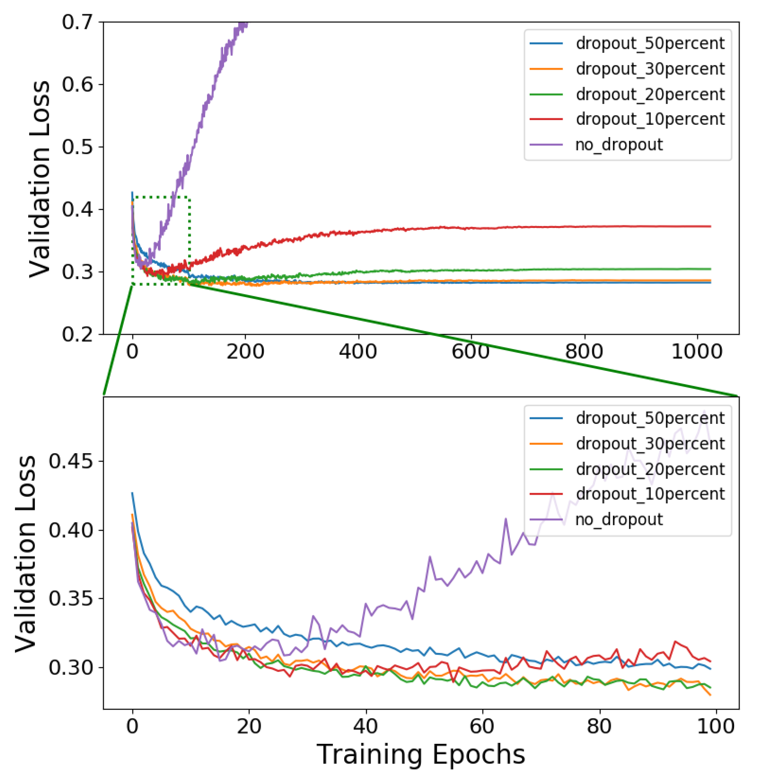
4.1. Classification

The performance of bnn-c is compared with some of the benchmark models listed in Table 4. We followed a 10-fold cross-validation method, and the means are reported in Table 4. From the results, we can infer that bnn-c produces a classification accuracy that is 4.88% better than the k-nearest neighbor method, the best among the benchmark models. The performance metric known as the receiver operating characteristic curve (ROC), which measures the classification capability of models at different classification thresholds, was obtained for the models. The area under the receiver operating characteristic curve (AUROC), which grades the classification capability of different models, was also calculated. From Table 4, it can be observed that the AUROC for bnn-c is 6.89% better than the best AUROC among the benchmark models. In addition, we tried different network layouts, and it was observed that the layout (117-117-117-1) improved the classification accuracy of bnn-c by 1.65%. The results are summarized in Table 5.
Figure 2 shows the loss curves obtained for the network architecture of (117-117-117-1), the Adam optimizer, and various degrees of dropout. We can observe that adding dropouts to the hidden layers improves the classification accuracy significantly. The results are summarized in Table 6. A dropout of 20% implemented on the hidden layers improves the classification accuracy by 2.9%. We followed a 6-fold cross-validation method with a dropout of 20% and an architecture of (117-117-117-1). The network accuracy is 88.28% with a standard deviation of 0.44%.
The classification unit, which was trained by the ChemClassA dataset configured for T = 10%, predicted 71,030 heuristic formation energies (out of 420,152 formation energies calculated for ChemClassB compounds) as accurate. It should be noted that these 71,030 formation energies correspond to 56,591 ternary compounds, as there was more than one formation energy for certain compounds. The classifier unit trained on the ChemClassA dataset with T = 5% labeled 28,715 formation energies (corresponding to 24,466 ternary compounds) as accurate. It is noted that in the first step, some combinations of elements are added to the ChemClassB dataset that do not exist in the MPD. For example, there is no ternary compound with H, Ir, and N elements available in the MPD. However, the heuristic formation energies of ternary compounds with these elements are available in the ChemClassB dataset. The training dataset used for the regression unit consists of the formation energies of ChemClassA compounds plus the formation energies of ChemClassB compounds that were labeled as accurate. By this means, the size of the dataset was increased from 40,049 to 96,640 for T = 10%. This corresponds to an increase of approximately 141% in the size of the data points. For T = 5%, the number of data points was increased by about 101% (from 24,466 entries to 49,345 entries).

4.2. Regression

The regression unit predicts the formation energies of ternary compounds whose heuristic formation energies cannot be calculated (240,248 compounds) or whose heuristic formation energies are not classified as accurate (229,821 and 197,696 ternary compounds for tolerances of 5% and 10%, respectively). For validation, we used the ternary compounds whose DFT-calculated formation energies are available but for whom the heuristic formula does not predict the formation energy accurately (7601 and 6231 compounds for T = 5% and T = 10%, respectively).
We compare the best five results of the regression unit in Table 7. In Ref. [29], the best MAE was 0.129 eV/atom, whereas we achieved an MAE of 0.114 eV/atom. Especially noteworthy is the size of the NNs used to achieve these results. In Ref. [29], several network layouts were tested, and a layout of (36-512-256-128-64-1), which has almost 200,000 learnable parameters, yielded the best results. Here, the network with the best results has only 2371 learnable parameters using a layout of (36-50-10-1). Compared to the training parameters of Ref. [29], our best network uses different activation and loss functions as well as a constant learning rate. On average, cAdam shows improvement over Adam, being better in 58% of the tested settings. However, the improvement is minor and comes at the cost of, on average, 47% longer training time. The Adam variant comparison in Ref. [21] shows that this longer computing time is due to the implementation through the Tensorflow API. A recreation of Adam in the same way also runs significantly slower than the default version in Tensorflow.

4.3. MNIST Classifier

The best five results of the MNIST classifier are summarized in Table 8. Our best-performing network on the MNIST dataset has a layout of (784-50-1-10), which has about 40,000 learnable parameters. The networks listed in Ref. [30] with a similar setup and performance have at least 300 hidden neurons, resulting in 200,000 to 500,000 learnable parameters. This significant difference in the number of learnable parameters can be explained by the findings in Ref. [31]. They introduce the intrinsic dimension of a model for a given problem, which describes the minimum number of parameters needed to reach a given accuracy. The number of parameters required to reach an accuracy of 90% for the MNIST dataset is about 750 [31]. The networks discussed here significantly surpass this number, so we can expect good results even with smaller networks. While [31] also shows that more parameters do tend to allow for better results, the gained performance becomes very small quite quickly. The extra computation time required for larger networks might be better spent on hyperparameter optimization or training for more epochs. In this experiment, cAdam performs better than Adam on 66% of the parameter settings at a cost of a 40% increase in training time. The differences in maximum accuracy, however, are small (see Table 8). Further analysis of results can be found in Ref. [21].

5. Summary

We proposed a two-step method to predict the formation energy of ternary compounds. The goal of the first unit, which is a classifier, is to increase the training dataset size for the second unit, which is a regression model to predict the formation energies. Based on available data in the MPD, a heuristic calculates the formation energies of ternary compounds, which are evaluated by the classifier. In this way, we increase the size of the training dataset for the regressor unit by at least 100%. Using a layout of (36-50-10-1) with the cAdam optimizer for the regression unit, an MAE of 0.114 eV/atom is achieved. The introduced optimizer cAdam, when trained on the MNIST dataset, yielded very similar results to Adam at a slightly higher computational cost.

Author Contributions

This work is based on the master thesis of V.R. and the bachelor thesis of S.J. Conceptualization H.M. Writing - Review & Editing, F.B., C.P., A.W. and T.D.K. All authors have read and agreed to the published version of the manuscript.

Funding

This work was partly funded by the Deutsche Forschungsgemeinschaft (DFG, German Research Foundation) under Germany’s Excellence Strategy as part of the project Berlin Mathematics Research Center MATH+ (EXC-2046/1, project ID: 390685689).

Data Availability Statement

Our models and data are available on GitHub: https://github.com/hmhoseini/Two-step-ML (accessed on 4 May 2023).

Acknowledgments

The authors gratefully acknowledge the computing time provided to them on the high-performance computers Noctua1 at the NHR Center in Paderborn (PC2). These are funded by the German Ministry of Education and Research, along with the German state governments participating in this national high-performance computing (NHR) project approved by the GWK.

Conflicts of Interest

The authors declare no conflict of interest.

Appendix A. Descriptors

Appendix A.1. Classification

We used 117 descriptors for the dataset of the classification model. The descriptors were created to capture the chemical properties of the binary and ternary compounds. The units of the descriptor are noted the first time that they are defined. The term “Average” refers to the composition-based weighted average of a property of the compound across its constituent elements. For example, for a ternary A x B y C z , if x = 0.4 and y = z = 0.3, then the average Pauling electronegativity of the ternary compound is
χ ( A 0.4 B 0.3 C 0.3 ) = 0.4 × χ A + 0.3 × χ B + 0.3 × χ C ,
where χ A denotes the Pauling electronegativity of element A. The term “Ratio” refers to the ratio of the property of each constituent element to the average value of the property of the compound. For example, for A 0.4 B 0.3 C 0.3 , the ratio of Pauling electronegativity for element A is
χ A χ ( A 0.4 B 0.3 C 0.3 ) .
The descriptors representing the ternary compound are as follows:
  • Heuristic formation energy: heuristically computed formation energy of the ternary compound (eV/atom);
  • Average Pauling electronegativity: average of the Pauling electronegativity values of the constituent elements of the ternary compound;
  • Average group on the periodic table: average of the group numbers of the elements;
  • Average row on the periodic table: average of the row numbers of the elements;
  • Average atomic mass: average of the atomic mass values of the constituent elements of the ternary compound (u);
  • Average ionic radius: average of the ionic radius values of the constituent elements of the ternary compound (Å);
  • Average electron affinity: average of the electron affinity values of the constituent elements of the ternary compound (eV);
  • Average first ionization energy: average of the first ionization energy values of the constituent elements of the ternary compound (eV);
  • Average van der Waals radius: average of the van der Waals radius values of the constituent elements of the ternary compound (Å);
  • Ratio of the electronegativity of each element in the compound to the average value of electronegativity of the ternary compound;
  • Ratio of the group number of each constituent element to the average for the ternary compound;
  • Ratio of the row number of each constituent element to the average for the ternary compound;
  • Ratio of the atomic mass of each constituent element to the average for the ternary compound;
  • Ratio of the ionic radius of each constituent element to the average for the ternary compound;
  • Ratio of the electron affinity of each constituent element to the average for the ternary compound;
  • Ratio of the first ionization energy of each constituent element to the average for the ternary compound;
  • Ratio of the van der Waals radius of each constituent element to the average for the ternary compound;
  • Orbital fraction of valence electrons s: ratio of the number of s electrons to the sum of the average of all electrons s , p , d , f of the ternary compound;
  • Orbital fraction of valence electrons p: ratio of the number of p electrons to the sum of the average of all electrons s , p , d , f of the ternary compound;
  • Orbital fraction of valence electrons d: ratio of the number of d electrons to the sum of the average of all electrons s , p , d , f of the ternary compound;
  • Orbital fraction of valence electrons f: ratio of the number of f electrons to the sum of the average of all electrons s , p , d , f of the ternary compound.
The descriptors representing a binary compound are:
  • Weight: the percentage of a binary compound’s formation energy that contributes to the formation energy of the ternary compound;
  • Formation energy: the formation energy of the binary constituent of the ternary compound;
  • Ratio of anions to cations: ratio of the number of anions to the number of cations in a binary compound;
  • Ratio of the cations in a constituent binary compound to its number in the ternary compound;
  • Ratio of the anions in a constituent binary compound to its number in the ternary compound;
  • Average Pauling electronegativity: average of the Pauling electronegativities of the constituent elements of the binary compound;
  • Average group on the periodic table: average of the group number of constituent elements;
  • Average row on the periodic table: average of the row number of constituent elements;
  • Average atomic mass: average of the atomic masses of the constituent elements of the binary compound;
  • Average ionic radius: average of the ionic radii of the constituent elements of the binary compound;
  • Average electron affinity: average of the electron affinity values of the constituent elements of the binary compound;
  • Average first ionization energy: average of the first ionization energy values of the constituent elements;
  • Average van der Waals radius: average of the van der Waals radius values of the constituent elements;
  • Absolute difference in the Pauling electronegativity of the constituent elements;
  • Absolute difference in the group number of the constituent elements;
  • Absolute difference in the row number of the constituent elements;
  • Absolute difference in the atomic mass of the constituent elements;
  • Absolute difference in the ionic radius of the constituent elements;
  • Absolute difference in the electron affinity value of the constituent elements;
  • Absolute difference in the first ionization energy of the constituent elements;
  • Absolute difference in the van der Waals radius of the constituent elements;
  • Difference in the group number of the constituent elements;
  • Difference in the row number of the constituent elements;
  • Difference in the atomic mass of the constituent elements;
  • Difference in the ionic radius of the constituent elements;
  • Difference in the electron affinity value of the constituent elements;
  • Difference in the first ionization energy of the constituent elements;
  • Difference in the van der Waals radius of the constituent elements;
  • Ratio of the Pauling electronegativity of the cations to that of the anions;
  • Ratio of the group number of the cations to that of the anions;
  • Ratio of the row number of the cations to that of the anions;
  • Ratio of the atomic mass of the cations to that of the anions;
  • Ratio of the ionic radius of the cations to that of the anions;
  • Ratio of the electron affinity of the cations to that of the anions;
  • Ratio of the first ionization energy of the cations to that of the anions;
  • Ratio of the van der Waals radius of the cations to that of the anions;
  • Orbital fraction of valence electrons s: ratio of the number of s electrons to the sum of the average of all electrons s , p , d , f of the binary compound;
  • Orbital fraction of valence electrons p: ratio of the number of p electrons to the sum of the average of all electrons s , p , d , f of the binary compound;
  • Orbital fraction of valence electrons d: ratio of the number of d electrons to the sum of the average of all electrons s , p , d , f of the binary compound;
  • Orbital fraction of valence electrons f: ratio of the number of f electrons to the sum of the average of all electrons s , p , d , f of the binary compound.

Appendix A.2. Regression

Analogous to the descriptors used in the classification model, the descriptors used for regression are chosen in such a way that they capture the chemical properties of the ternary compound. The descriptors are:
  • Average Pauling electronegativity: the average of the Pauling electronegativity values of the constituent elements of the ternary compound;
  • Average group on the periodic table: average of the group numbers of the constituent elements;
  • Average row on the periodic table: average of the row numbers of the constituent elements;
  • Average atomic mass: average of the atomic masses of the constituent elements;
  • Average ionic radius: average of the ionic radii of the constituent elements;
  • Average electron affinity: average of the electron affinity values of the constituent elements;
  • Average first ionization energy: average of the first ionization energies of the constituent elements;
  • Average van der Waals radius: average of the van der Waals radii of the constituent elements;
  • Ratio of the electronegativity of each element in the compound to the average value of the electronegativity of the ternary compound;
  • Ratio of the group number of each element in the compound to the average value of the group number of the ternary compound;
  • Ratio of the row number of each element in the compound to the average value of the row number of the ternary compound;
  • Ratio of the atomic mass of each element in the compound to the average value of the atomic mass of the ternary compound;
  • Ratio of the ionic radius of each element in the compound to the average value of the ionic radius of the ternary compound;
  • Ratio of the electron affinity of each element in the compound to the average value of the electron affinity of the ternary compound;
  • Ratio of the first ionization energy of each element in the compound to the average value of the first ionization energy of the ternary compound;
  • Ratio of the van der Waals radius of each element in the compound to the average value of the van der Waals radius of the ternary compound;
  • Orbital fraction of valence electrons s: the ratio of the number of s electrons to the sum of the average of all electrons s , p , d , f of the ternary compound;
  • Orbital fraction of valence electrons p: the ratio of the number of p electrons to the sum of the average of all electrons s , p , d , f of the ternary compound;
  • Orbital fraction of valence electrons d: the ratio of the number of d electrons to the sum of the average of all electrons s , p , d , f of the ternary compound;
  • Orbital fraction of valence electrons f: the ratio of the number of f electrons to the sum of the average of all electrons s , p , d , f of the ternary compound.

Appendix B. Dataset and Preprocessing

MNIST

MNIST is a dataset commonly used for comparing neural networks. It contains grayscale images of handwritten digits from 0 to 9 as well as corresponding integer labels. Each input is a 28 × 28 matrix of integer values in the interval from 0 to 255. The dataset contains 60,000 training images and 10,000 dedicated test images.
For training, the integer values of the inputs were scaled to the interval 0 , 1 R by dividing by 255. The labels of the dataset were integers in the range 0 , 9 . Those were one-hot encoded such that each label was a vector v 0 , 1 10 with v = 1 . Every integer in the original labels corresponds to one position in these vectors.
Examples:
2 0 , 0 , 1 , 0 , 0 , 0 , 0 , 0 , 0 , 0 ;
5 0 , 0 , 0 , 0 , 0 , 1 , 0 , 0 , 0 , 0 .

Appendix C. Computational Resources

Experiments were conducted on a Macbook Pro with an Intel Core i5-3210M processor and a CPU @ 2.50 GHz with 3 GB system memory.
The experiments with cAdam on the ChemRegA dataset were conducted on an ASUS Flow X13 (2022) laptop with an AMD Ryzen 6800HS CPU and NVIDIA RTX 3050 GPU with 16 GB system memory. The resulting data for the test of cAdam on the MNIST dataset were taken from Ref. [21], and the result summary was recalculated.

References

  1. Morgan, D.; Ceder, G.; Curtarolo, S. High-throughput and data mining with ab initio methods. Meas. Sci. Technol. 2004, 16, 296. [Google Scholar] [CrossRef]
  2. Li, W.; Jacobs, R.; Morgan, D. Predicting the thermodynamic stability of perovskite oxides using machine learning models. Comput. Mater. Sci. 2018, 150, 454–463. [Google Scholar] [CrossRef]
  3. Schmidt, J.; Chen, L.; Botti, S.; Marques, M.A.L. Predicting the stability of ternary intermetallics with density functional theory and machine learning. J. Chem. Phys. 2018, 148, 241728. [Google Scholar] [CrossRef] [PubMed]
  4. Davies, D.; Butler, K.; Jackson, A.; Morris, A.; Frost, J.; Skelton, J.; Walsh, A. Computational Screening of All Stoichiometric Inorganic Materials. Chem 2016, 1, 617–627. [Google Scholar] [CrossRef] [PubMed]
  5. Meredig, B.; Agrawal, A.; Kirklin, S.; Saal, J.E.; Doak, J.W.; Thompson, A.; Zhang, K.; Choudhary, A.; Wolverton, C. Combinatorial screening for new materials in unconstrained composition space with machine learning. Phys. Rev. B 2014, 89, 094104. [Google Scholar] [CrossRef]
  6. Liu, R.; Ward, L.; Wolverton, C.; Agrawal, A.; Liao, W.; Choudhary, A. Deep learning for chemical compound stability prediction. In Proceedings of the ACM SIGKDD Workshop on Large-Scale Deep Learning for Data Mining (DL-KDD), San Francisco, CA, USA, 13–17 August 2016; pp. 1–7. [Google Scholar]
  7. Jha, D.; Ward, L.; Paul, A.; Liao, W.k.; Choudhary, A.; Wolverton, C.; Agrawal, A. ElemNet: Deep Learning the Chemistry of Materials From Only Elemental Composition. Sci. Rep. 2018, 8, 17593. [Google Scholar] [CrossRef] [PubMed]
  8. Xie, T.; Grossman, J.C. Crystal Graph Convolutional Neural Networks for an Accurate and Interpretable Prediction of Material Properties. Phys. Rev. Lett. 2018, 120, 145301. [Google Scholar] [CrossRef] [PubMed]
  9. Schütt, K.T.; Kessel, P.; Gastegger, M.; Nicoli, K.A.; Tkatchenko, A.; Müller, K.R. SchNetPack: A Deep Learning Toolbox For Atomistic Systems. J. Chem. Theory Comput. 2019, 15, 448–455. [Google Scholar] [CrossRef] [PubMed]
  10. Choudhary, K.; DeCost, B. Atomistic Line Graph Neural Network for improved materials property predictions. npj Comput. Mater. 2021, 7, 185. [Google Scholar] [CrossRef]
  11. Wang, A.Y.T.; Murdock, R.J.; Kauwe, S.K.; Oliynyk, A.O.; Gurlo, A.; Brgoch, J.; Persson, K.A.; Sparks, T.D. Machine Learning for Materials Scientists: An Introductory Guide toward Best Practices. Chem. Mater. 2020, 32, 4954–4965. [Google Scholar] [CrossRef]
  12. Peterson, G.G.C.; Brgoch, J. Materials discovery through machine learning formation energy. J. Phys. Energy 2021, 3, 022002. [Google Scholar] [CrossRef]
  13. Kirklin, S.; Saal, J.E.; Meredig, B.; Thompson, A.; Doak, J.W.; Aykol, M.; Rühl, S.; Wolverton, C. The Open Quantum Materials Database (OQMD): Assessing the accuracy of DFT formation energies. npj Comput. Mater. 2015, 1, 15010. [Google Scholar] [CrossRef]
  14. Reiser, P.; Neubert, M.; Eberhard, A.; Torresi, L.; Zhou, C.; Shao, C.; Metni, H.; van Hoesel, C.; Schopmans, H.; Sommer, T.; et al. Graph neural networks for materials science and chemistry. Commun. Mater. 2022, 3, 93. [Google Scholar] [CrossRef] [PubMed]
  15. Yan, K.; Liu, Y.; Lin, Y.; Ji, S. Periodic Graph Transformers for Crystal Material Property Prediction. In Proceedings of the 36th Annual Conference on Neural Information Processing Systems, New Orleans, LA, USA, 28 November–9 December 2022. [Google Scholar]
  16. Jain, A.; Ong, S.P.; Hautier, G.; Chen, W.; Richards, W.D.; Dacek, S.; Cholia, S.; Gunter, D.; Skinner, D.; Ceder, G.; et al. The Materials Project: A materials genome approach to accelerating materials innovation. APL Mater. 2013, 1, 011002. [Google Scholar] [CrossRef]
  17. Chen, C.; Ye, W.; Zuo, Y.; Zheng, C.; Ong, S.P. Graph Networks as a Universal Machine Learning Framework for Molecules and Crystals. Chem. Mater. 2019, 31, 3564–3572. [Google Scholar] [CrossRef]
  18. Hillert, M. Phase Equilibria, Phase Diagrams and Phase Transformations: Their Thermodynamic Basis, 2nd ed.; Cambridge University Press: Cambridge, UK, 2007. [Google Scholar] [CrossRef]
  19. Muggianu, Y.M.; Gambino, M.; Bros, J. Enthalpies of formation of liquid alloys bismuth-gallium-tin at 723k-choice of an analytical representation of integral and partial thermodynamic functions of mixing for this ternary-system. J. Chim. Phys. Phys.-Chim. Biol. 1975, 72, 83–88. [Google Scholar] [CrossRef]
  20. Kingma, D.P.; Ba, J. Adam: A Method for Stochastic Optimization. In Proceedings of the 3rd International Conference on Learning Representations, ICLR 2015, San Diego, CA, USA, 7–9 May 2015. Conference Track Proceedings; 2015. [Google Scholar]
  21. Jost, S. Comparison of Architectures and Parameters for Artificial Neural Networks. 2021. Available online: https://github.com/simulatedScience/Bachelorthesis (accessed on 4 May 2023).
  22. Chollet, F. Keras. 2015. Available online: https://keras.io (accessed on 4 May 2023).
  23. Abadi, M.; Agarwal, A.; Barham, P.; Brevdo, E.; Chen, Z.; Citro, C.; Corrado, G.S.; Davis, A.; Dean, J.; Devin, M.; et al. TensorFlow: Large-Scale Machine Learning on Heterogeneous Systems. 2015. Available online: https://www.tensorflow.org/ (accessed on 4 May 2023).
  24. Pedregosa, F.; Varoquaux, G.; Gramfort, A.; Michel, V.; Thirion, B.; Grisel, O.; Blondel, M.; Prettenhofer, P.; Weiss, R.; Dubourg, V.; et al. Scikit-learn: Machine Learning in Python. J. Mach. Learn. Res. 2011, 12, 2825–2830. [Google Scholar]
  25. Van der Walt, S.; Colbert, S.C.; Varoquaux, G. The NumPy array: A structure for efficient numerical computation. Comput. Sci. Eng. 2011, 13, 22–30. [Google Scholar] [CrossRef]
  26. Jones, E.; Oliphant, T.; Peterson, P. SciPy: Open Source Scientific Tools for Python. 2001. Available online: http://www.scipy.org (accessed on 4 May 2023).
  27. McKinney, W. Data Structures for Statistical Computing in Python. In Proceedings of the 9th Python in Science Conference, Austin, TX, USA, 28 June–3 July 2010; pp. 51–56. [Google Scholar]
  28. Hunter, J.D. Matplotlib: A 2D graphics environment. Comput. Sci. Eng. 2007, 9, 90–95. [Google Scholar] [CrossRef]
  29. Rengaraj, V. A Two-Step Machine Learning for Predicting the Stability of Chemical Compositions. Master’s Thesis, Paderborn University, Paderborn, Germany, 2019. [Google Scholar]
  30. LeCun, Y.; Cortes, C. MNIST Handwritten Digit Database. 2010. Available online: http://yann.lecun.com/exdb/mnist/ (accessed on 4 May 2023).
  31. Li, C.; Farkhoor, H.; Liu, R.; Yosinski, J. Measuring the Intrinsic Dimension of Objective Landscapes. In Proceedings of the 6th International Conference on Learning Representations, ICLR 2018, Vancouver, BC, Canada, 30 April–3 May 2018. [Google Scholar]
Figure 1. Diagram representing the two-step ML approach to predict the formation energies of the ternary compounds. (a) The classification unit to predict if the heuristically computed formation energy of a ternary compound is accurate or not. (b) The regression unit to predict the formation energy of a ternary compound.
Computation 11 00095 g001
Figure 2. Loss curves obtained for the network architecture of (117-117-117-1), the Adam optimizer, and various degrees of dropout.
Computation 11 00095 g002
Table 1. Configuration of the baseline NN, bnn-c, for the classification.
Model Parameters
   Activation function H i d d e n    ReLU
   Activation function O u t p u t    Sigmoid
   Configuration   117-117-1
   Loss function   Binary cross-entropy
   Training parameters
   Batch size   128
   Training cycles   512
   Validation split   0.1
   Test split   0.1
   Optimizer parameters
   Optimizer   Adam
   Learning rate   0.001
    ε     1 / 10 7
    β 1    0.9
    β 2    0.999
Table 2. NN parameters for the regression task.
Model Parameters
   Activation function H i d d e n    ReLU/Sigmoid
   Activation function O u t p u t    Linear
   configuration    36 40 20 1 /
    36 50 10 1 /
    36 30 30 10 1
   Loss function   Log cosh/Mean squared error
Training parameters
   Batch size   100/1000/10,000
   Training cycles   500
   Validation split   0.2
   Optimizer parameters
   Optimizer   Adam/cAdam
   Learning rate   0.01/0.001
    ε     10 7
    β 1    0.9
    β 2    0.999
Table 3. NN parameters for MNIST.
Model Parameters
   Activation function H i d d e n    ReLU/Sigmoid
   Activation function O u t p u t    Softmax/Sigmoid
   configuration    784 32 10 /
    784 50 10 10 /
    784 20 15 10 10
   Loss function   Categorical cross-entropy/
   Mean squared error
Training parameters
   Batch size   100/1000/10,000
   Training cycles   5/25/50
   Validation split   0.2
   Optimizer parameters
   Optimizer   Adam/cAdam
   Learning rate   0.1/0.01/0.001
    ε    1/ 10 7
    β 1    0.9
    β 2    0.999
Table 4. Performance of bnn-c compared with conventional ML classifiers: logistic regression (LR), linear discriminant analysis (LDA), random forest (RF), k-nearest neighbors (KNN), and adaboost (AB).
ModelAccuracyPrecisionRecallAUROC
LR0.790.730.570.85
LDA0.790.720.560.85
KNN0.820.720.680.86
RF0.740.740.290.72
AB0.810.740.630.87
bnn-c0.860.780.770.93
Table 5. Performance comparison between bnn-c (first row) and modified NN configurations.
LayoutAccuracy (%)PrecisionRecallAUROC
117-117-186.920.790.780.93
117-300-187.140.780.800.93
117-55-186.250.770.790.93
117-117-117-187.420.810.780.93
117-117-117-117-187.060.800.770.93
Table 6. Results obtained for the network architecture of (117-117-117-1) with various degrees of dropouts.
Dropout in %Accuracy (%)PrecisionRecallAUROC
5087.820.860.720.93
3088.240.820.790.94
2088.290.840.770.94
1088.510.830.780.94
Table 7. The best 5 of the 144 parameter combinations and results for the regression task. The units for the MAE values are eV/atom. Results are sorted by final validation loss.
ParameterBest Values
Final val loss (MAE)0.11160.112080.114160.114930.11534
Test loss (MAE)0.113890.112980.114930.114450.11539
Test loss0.0129710.0127640.00659030.00653540.0066426
Training time (in s)44.379566.85577.9280.44744.17
Neurons per layer(50, 10)(50, 10)(50, 10)(30, 30, 10)(40, 20)
Activation functionsSigmoidSigmoidSigmoidSigmoidSigmoid
Last activation functionLinearLinearLinearLinearLinear
Loss functionMSEMSELog coshLog coshLog cosh
Number of epochs500500500500500
Batch size100010010010001000
OptimizerAdamcAdamcAdamcAdamAdam
Learning rate0.010.0010.0010.010.01
ε 10 7 10 7 10 7 10 7 10 7
Table 8. The best 5 of the 2592 parameter combinations and results for NNs trained on the MNIST dataset. Results are sorted by final validation accuracy. Every network was trained five times, and the average values are listed.
ParameterBest Values
Final validation accuracy0.970.96910.969050.968850.9688
Test accuracy0.970060.969060.96810.970480.97084
Final validation loss0.013390.00669570.014490.00705070.96845
Training time (in s)46.66643.60286.10586.87423.122
Neurons per layer 50 , 10 50 , 10 50 , 10 50 , 10 50 , 10
Activation function H i d d e n ReLUReLUReLUReLUReLU
Activation function O u t p u t SigmoidSigmoidSigmoidSoftmaxSoftmax
Loss functionCat-crossCat-crossCat-crossCat-crossCat-cross
Training cycles5025505025
Batch size100100100100100
OptimizerAdamcAdamcAdamcAdamAdam
Learning rate0.0010.10.10.10.1
ε 10 7 1.01.01.01.0
Disclaimer/Publisher’s Note: The statements, opinions and data contained in all publications are solely those of the individual author(s) and contributor(s) and not of MDPI and/or the editor(s). MDPI and/or the editor(s) disclaim responsibility for any injury to people or property resulting from any ideas, methods, instructions or products referred to in the content.

