

Modelling Qualitative Data from Repeated Surveys

Department of Political Sciences, University of Naples Federico II, Via L. Rodinò 22, 80138 Naples, Italy
*
Author to whom correspondence should be addressed.
Computation 2023, 11(3), 64; https://doi.org/10.3390/computation11030064
Submission received: 31 December 2022
/
Revised: 4 March 2023
/
Accepted: 8 March 2023
/
Published: 20 March 2023
(This article belongs to the Special Issue Computational Issues in Insurance and Finance)
Abstract
:This article presents an innovative dynamic model that describes the probability distributions of ordered categorical variables observed over time. For this purpose, we extend the definition of the mixture distribution obtained from the combination of a uniform and a shifted binomial distribution (CUB model), introducing time-varying parameters. The model parameters identify the main components ruling the respondent evaluation process: the degree of attraction towards the object under assessment, the uncertainty related to the answer, and the weight of the refuge category that is selected when a respondent is unwilling to elaborate a thoughtful judgement. The method provides a tool to quantify the data from qualitative surveys. For illustrative purposes, the dynamic CUB model is applied to the consumers’ perceptions and expectations of inflation in Italy to investigate: (a) the effect of the COVID pandemic on inflation beliefs; (b) the impact of income level on respondents’ expectations.
1. Introduction
Business and consumer survey data are the basis for several indicators describing the trend of macro-economic variables that are fundamental for monitoring the overall performance of the economic system. Qualitative surveys typically ask interviewees to express their perceptions or expectations about the current or future tendency of a reference economic variable (such as inflation or industrial output) using a trichotomous or a fine-tuned ordered scale. Surveys are carried out at regular interval by statistical offices and the collected data are traditionally published in aggregate form, reporting the proportions of positive, neutral or negative assessments. Given the level of data aggregation, the methods relying on the individual responses and covariates describing the panel of respondents are of limited use [1]. Thus, many studies in the literature have investigated how these proportions could be converted into a quantitative measure of the perceived or expected development of an economic variable. Among the earliest contributions, the balance statistic of the frequencies of positive and negative responses, due to Theil [2], the probability method of Carlson and Parkin [3], and the regression approach [4], have been widely applied in empirical studies and have stimulated several developments (see [5] for an overview). Recently, attention has been focused on the use of time-series models for proportions of respondents falling in each response category over time. In this vein, ref. [6] proposed two methods. The first one is a non-parametric method based on a spectral envelope that helps to estimate the linear combination of the proportions. The second one, instead, extracts the latent cycle from the multivariate time series of proportions by means of a parametric dynamic cumulative logit model.
This article presents an innovative dynamic model that describes the probability distributions of an ordered categorical variable observed over time. We suggest the use of model time-varying parameters as indicators of the diversity of respondents’ opinions, shifting from an optimistic to a pessimistic state as the economic situation evolves.
For this aim, we extend the well-established CUB model [7,8,9]. The acronym denotes a univariate mixture distribution, defined by the convex combination of a uniform and a shifted binomial distribution, that mimics a simplified mechanism of judgement formation. In particular, this mechanism is ruled by two unobserved components denoted as feeling and uncertainty. The former describes the respondents’ latent attitude towards the object of evaluation. The latter conveys the uncertainty of the evaluation process, caused by the difficulties that respondents’ experience when they have to bring their opinions into focus and summarize them into a well-defined category [10]. In this regard, refs. [8,11] discussed the main features and advantages of the CUB model compared with those embedded in the GLM (generalized linear model) class (i.e., cumulative models). These advantages include the parsimonious formulation (the estimation of cut-points is not needed), the meaning given to the parameters as elements of the rater choice mechanism, the wide range of graphical representations that support the interpretation of results and the possibility to solve discrimination and classification problems in the presence of multiple items.
When ordinal data are produced from repeated surveys, the temporal pattern of the uncertainty and feeling components represents how the shape of the distribution of the ordered categorical variables change over time. The initial suggestion on the use of CUB models for ordinal time series was made by [12] and has been further developed by [13]. However, these methods are based on a two-step procedure that requires the estimate of a CUB model at each instant separately. The parameter estimates are then collected into time series, which become the focus of further modelling. This article, instead, develops a direct approach that establishes an explicit link between the parameters of the dynamic CUB model and a number of explanatory variables. In this way, the time dependency between frequency distributions is preserved and directly modelled.
The dynamic CUB model offers a parsimonious parametric representation that can be used for various purposes. Firstly, the graph of the estimated time-varying parameters allows the identification of changes in respondents’ opinions and the evaluation of the impact of external economic shocks. In our view, this picture is more informative than studying the time series of summary statistics, such as the mean or median of the observed distributions [14]. Moreover, the pattern of the estimated time-varying parameters provides a characterization that helps to discover similarities among the opinions expressed on a given item by different groups of respondents.
The empirical case study in Section 3 shows how these aims can be achieved in practice using graphical representations of the uncertainty and feeling components. The study examines data from the consumer opinion surveys conducted regularly by the national statistical institute (ISTAT) as part of the Joint Harmonised EU Programme of Business and Consumer Surveys. Although, since 2010, quantitative inflation perceptions and expectations have been collected by national statistical institutes in Europe, respondents find it much easier to provide the direction of change in inflation rather than numerical estimates of such variation. This results in a consistent bias in the quantitative estimate of inflation [15]. For this reason, the statistical treatment of subjective judgements about current and future inflation is still a topic of considerable interest. In particular, the proposed model is applied to investigate the consumer perceptions and expectations about inflation in Italy considering: (a) the evolution of consumers’ beliefs during the COVID pandemic; (b) the disagreement between respondents with different income levels. The results show that: (a) the pandemic had a strong effect on consumer opinion formation, but that the impact was temporary; (b) disadvantaged people typically tended to expect a higher level of inflation and this propensity changed significantly over the years.
2. Method and Materials
2.1. The Dynamic CUB Model
We assume that the question aimed at identifying the respondent’s opinion or attitude towards a certain item is framed positively. Then, the individual responses are represented by means of ordered categories, attaching the lowest score to the worst judgement. Denoting with a collection of random variables describing the ordinal data observed at different time points, we characterize by means of the following probability mass distribution:
with:
where , and are vectors including the constant term and the values of lagged explanatory variables (predictors), is the set of information concerning these variables until time , and , and are vectors of parameters. Overall, the parameters are indicated with . The time-varying parameters satisfy the constraints: ; ; , for .
Finally, is a degenerate distribution with unit mass at the shelter category . This is a neutral or safe category that is selected by respondents who are careless, unwilling or unable to express a thoughtful judgement [10]. The presence of such a category is especially useful for modelling data from surveys addressed to non-experts (for example, households, entrepreneurs and small business owners). The choice process is then represented by a sort of c-inflated model. At a given time t, the respondent decides between giving a quick answer using the refuge category or undertaking deeper reflection about the question content. The two alternatives are selected with probability and , respectively. Due to the nature of the shelter category, it is reasonable to assume that c remains unchanged over time.
Once the respondent is willing to think more deeply, the judgement is driven by the feeling and uncertainty components. Specifically, at a given time t, the parameter characterizes the shifted binomial distribution. In particular, for given values of , and m, the skewness of the distribution is negative when . This implies that the larger , the larger is the probability that respondents attach a high rating to the item under evaluation. The opposite, instead, is verified when . For this reason, has been related to the latent attitude of respondents about the object of assessment and has been referred to as feeling. In practice, it denotes the degree of liking (disliking) of respondents, and, in general, the strength of the positive/negative rating attached to the item at a certain time t. The uncertainty is measured by that determines the contribution of the uniform distribution in the mixture at a given instant. When , the selection of categories is dominated by the ignorance or uncertainty of respondents to convey their judgements or opinions using the available rating scale. The uncertainty is related to the heterogeneity of the distribution [16] and, in this sense, represents the mutual disagreement among respondents.
Moreover, the parameter weights the shift in the mean operated by the shelter category at a given instant. It is straightforward to derive that:
with . In this regard, we recall that the widely used Theil’s balance statistic is the weighted difference in the proportions of respondents who report positive assessments versus those who report negative assessments. This can be related to the expected value of an ordinal variable whose values are equally spaced and symmetric. For example, assuming that , the balance at time t is , being the probability of responses in each category j. It is straightforward to show that . Then, using the fitted model (1), it is possible to explore the dependency of the balance statistics from the explanatory variables.
2.2. Estimation and Fitting Measure
The estimation of the model (1) can be performed by the minimum chi-square method (see [17,18] for a discussion). This seems to be a natural choice for the issue we are examining, because data arise in the form of frequency distributions of a periodically observed discrete random variable.
In particular, let be the relative frequencies from a random sample of n observations drawn from at a given instant, and assume that the sampling is repeated for different time points . Moreover, for brevity, let . Then, the minimum chi-square estimates of are obtained by minimizing:
The criterion (7) is a special case of more general divergence measures, such as the power divergence statistic introduced by [19] and the phi-divergence statistic discussed by [20], for which interesting properties and developments have been derived. Moreover, the minimum chi-square method achieves higher second-order efficiency with respect to the minimum modified chi-square method [21]. In addition, the minimum chi-square estimators are asymptotically normal with mean and asymptotic variance covariance matrix with [22]:
However, in empirical studies using official data from complex surveys, the number of interviewees may not be available. This is, for instance, the case for the dataset that will be analyzed in Section 3.2, where the opinions about the inflation trend expressed by groups of individuals are examined. The metadata concerning the European consumer survey reports the overall sample size and the sampling method, but it does not give details about the number of individuals allocated in the various strata. For this reason, in such a situation, we suggest using bootstrap to evaluate the standard errors of estimates and building confidence intervals about the time-varying parameters [23,24]. The procedure is implemented as follows:
- firstly, data are organized as a matrix, R, where rows are given by , ;
- a bootstrap sample is created by resampling T rows from R with replacement. This preserves the dependency of each ordinal distribution with the explicative variables;
- the bootstrap estimates of the parameters are evaluated by fitting the model (1) to the bootstrap sample;
- the bootstrap replicates of the time-varying parameter estimates are obtained using (3).
The process is repeated B times by obtaining the respective bootstrap cumulative distribution functions , , from which the standard errors and non-parametric confidence intervals are computed. In particular, considering for example , the bootstrap standard error of is obtained from:
where: . The confidence interval is where is the -th percentile of the bootstrap distribution (see [23] pp. 179–180).
Finally, the goodness of fit of the model can be evaluated by comparing with the discrepancy between the observed relative frequencies and the uniform probabilities:
The uniform distribution in (10) is representative of the worst model that could be fitted to the data because it reflects the situation of pure ignorance about the phenomenon under investigation. Then, the percentage decrease in the chi-square measures (denoted with ) will indicate how far the fitted model is from the ignorance model.
2.3. Data Description
A consumer confidence survey is carried out monthly by the Italian statistical office (ISTAT) within the EU programme of continuous surveys. The questionnaire includes questions, mainly qualitative, on the general economic situation in Italy and on the personal situation of the respondent. Opinions are expressed as assessments concerning the recent past or as expectations about the short-term future. Consumers are asked to answer, amongst others, two questions about their perceptions and expectation of inflation. The first one (denoted as Q5) concerns their perception of past inflation development, and is formulated as follows:
Q5. How do you think that consumer prices have developed over the last 12 months? They have: risen a lot; risen moderately; risen slightly; stayed about the same; fallen.
The second one polls, instead, the expectation about the future trend in inflation by asking:
Q6. By comparison with the past 12 months, how do you expect consumer prices will develop in the next 12 months? They will: increase more rapidly; increase at the same rate; increase at a slower rate; stay about the same; fall.
Only the frequency distributions of responses are published monthly. We denote with the ordinal variable representing the consumers’ perceptions, and with , the expectations. The observed categories are recoded so that 1 is associated to the category “fallen/fall”, and 5 to the category “risen a lot/increase more rapidly”. The shape of the distributions of the ordinal variable , associated to each time point, may vary depending on the economic situation.
Various drivers have been investigated in the literature as possible determinants of consumers’ inflation perceptions and expectations. A conceptual framework of the process generating individual’s opinions has been illustrated by [25]. In particular, this includes several acting forces, such as the socio-economic environment of respondents, personal attitudes (gender, age, personal income, level of education), and social amplification mechanisms due to news about the economy.
According to [26,27,28], consumers base their judgements and opinions about inflation development only on the most recent past, exhibiting short memory. Moreover, inflation expectations are related to perceptions. However, as suggested by various psychological experiments, this relationship is not one-way and, in addition, the influence is not only true from the present to the future. Expectations about price trends, formed at some previous time, may bias perceptions of the current situation [29,30,31].
These considerations have guided us in choosing two case studies to demonstrate implementation of the methodology. Firstly, we consider the impact of the COVID pandemic on consumers’ opinions about inflation trends in Italy. During the period of more drastic measures, the falling demand caused by the reduced opportunity for consumption and disruptions to supply chains produced opposite pressures on prices. In addition, sudden changes in consumer expenditure patterns introduced bias in the measurement of inflation based on consumer price indices [32,33]. Within this framework, monitoring consumers’ beliefs of current and future inflation was a challenging issue for monetary authorities and policy-makers [34,35] because the pandemic (and amplification due to news and social media) altered both perceptions and expectations about the development of inflation [36,37].
Secondly, we examine how opinions about future inflation change according to the income level of respondents. Using data from the Michigan survey of consumers, ref. [38] found that low-income people had significantly higher inflation expectations. Arioli [15] drew similar conclusions by analysing quantitative measures of expected inflation from the European consumer survey. Here, we show how the dynamic CUB model can detect different behaviour of consumers using aggregate data from qualitative surveys.
3. Results
3.1. The Effect of the COVID Pandemic on Consumers’ Opinions about Inflation
We consider consumers’ opinions about inflation (perceptions and expectations) in Italy from January 2018 to March 2021. Note that, in April 2020, the consumer and business confidence survey was suspended and resumed regularly from May. Moreover, from the end of February 2020, numerous containment measures were implemented by Italian authorities to cope with the spread of the pandemic. In particular, after the initial national lockdown (from 9 March to 4 May), Italy experienced a number of stop-and-go measures characterized by different levels of restriction in accordance with the growth of Covid cases (see, [39,40] for a discussion of control policies).
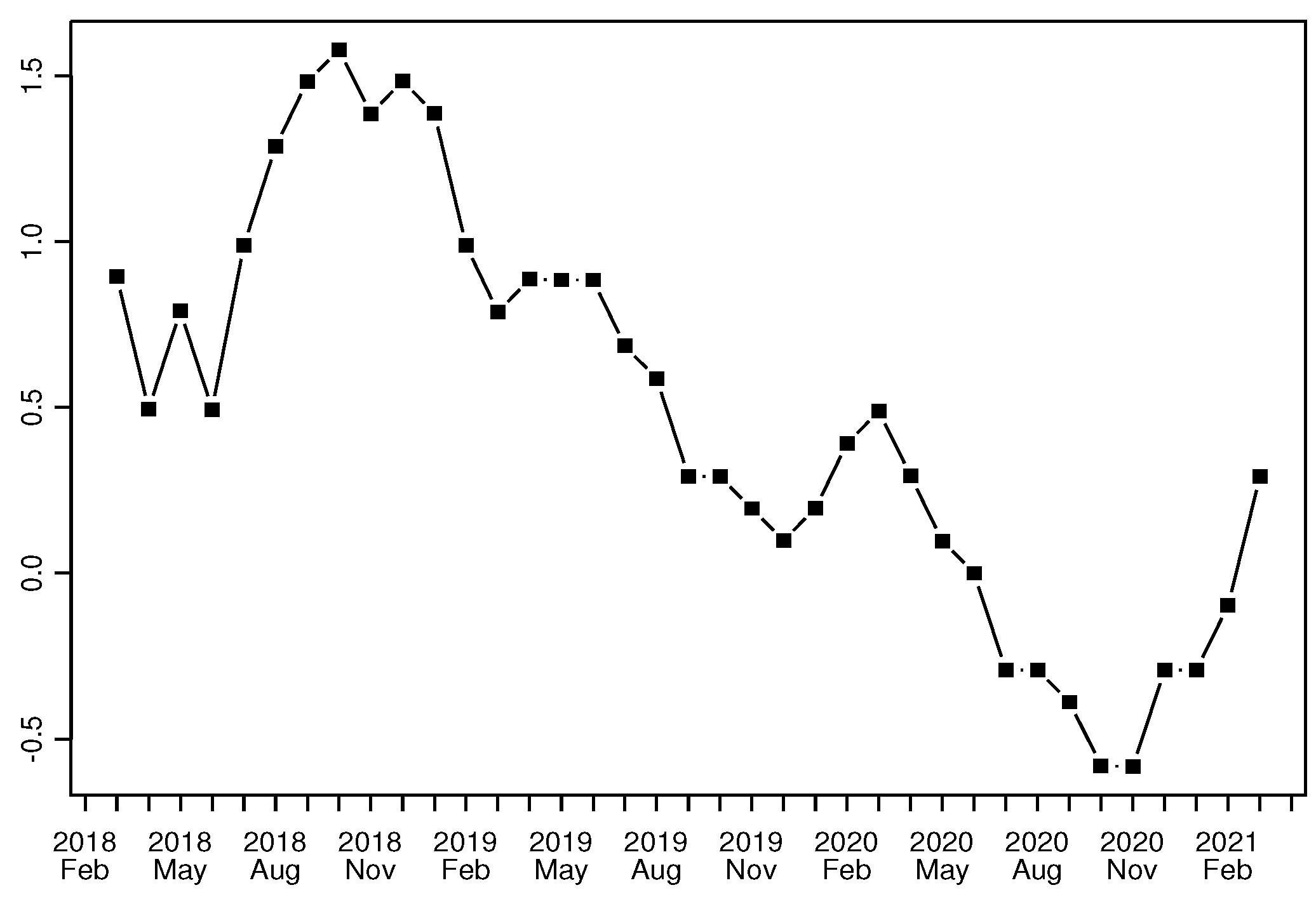
During this period, the year-on-year changes in the consumer price index declined remarkably due to weak consumer demand and persistent economic slowdown. From May 2020, the rate of inflation was negative and still declining. It only began to rise at the end of the year (Figure 1). At the same time, consumer perceptions were altered by the changed consumption basket [41] and shopping frequency [42], and by unfairness and steep changes in the prices of particular goods [25]. Moreover, expectations were influenced by growing concern about the evolution of the health crisis.
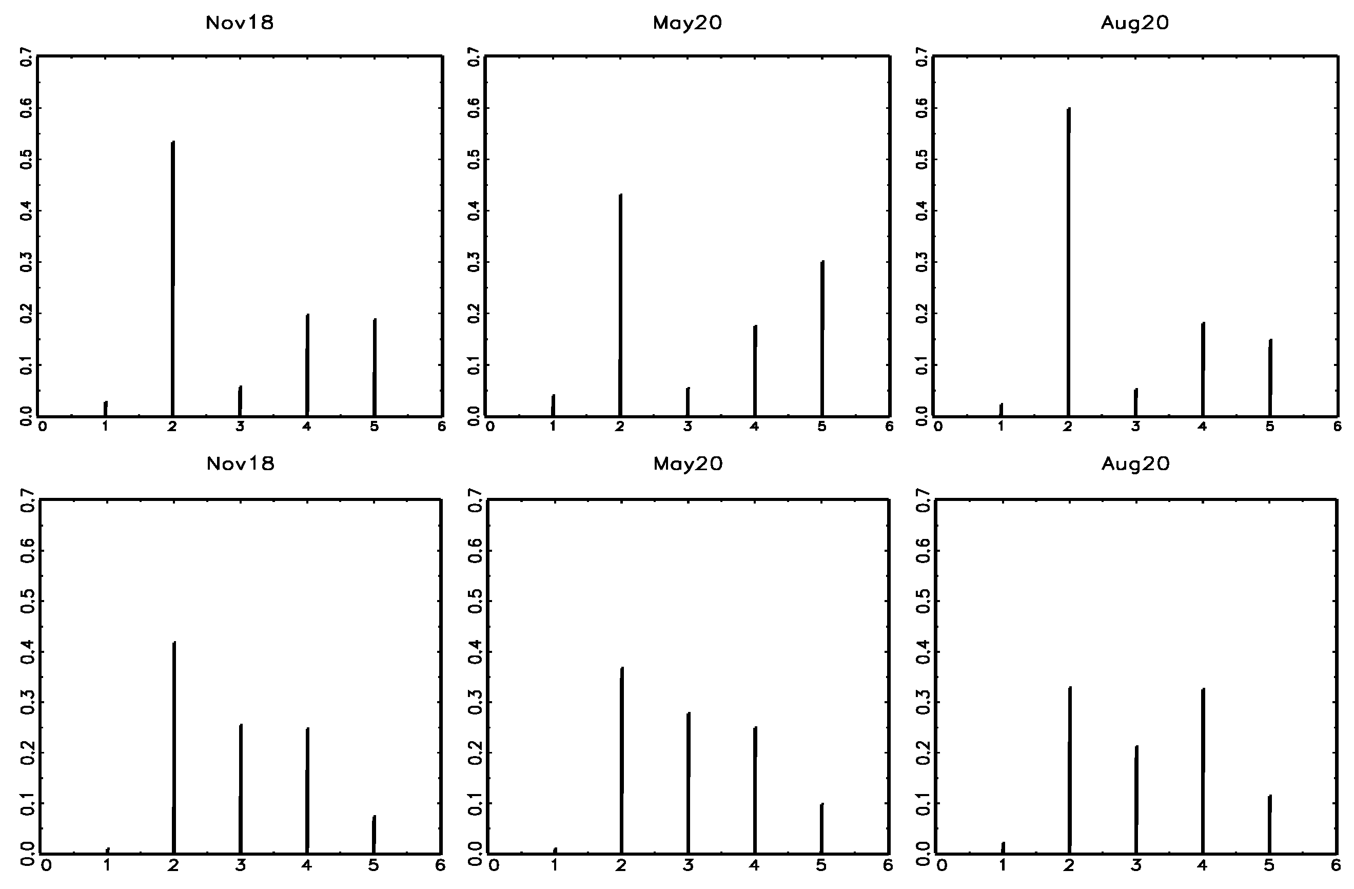
The frequency distributions of opinions observed over time present some common features, as illustrated in Figure 2 for a few selected time points. Firstly, a prominent peak is located at the neutral category, indicating that the level of prices has remained (or is expected to remain) about the same. For this reason, both models elaborated for inflation perceptions and expectations include a refuge category . Secondly, a lower peak, located at the categories indicating an increase (or an expected increase) in prices, is observed for most of the considered time points. Moreover, as discussed previously, consumer opinion formation is a short memory process [26,27,28] and inflation expectations and perceptions affect each other [29,30,31].
The model of inflation expectations is a mixture including the three components described in (1). The parameter depends on the mean of expectations at time (aveExp) and the parameter on the mean of perceptions at time (avePerc). These relationships represent a sort of inertia of the opinion formation process and mimics the availability heuristic that individuals use to elaborate their opinions [43]. The uncertainty in expressing opinions about future inflation may increases when, at the previous instant, a higher proportion of respondents believed that current inflation had increased. Similarly, the feeling may increase (so that a higher probability will be linked to rising inflation categories) when, in the previous instant, a higher proportion of respondents believed that inflation was going to increase. In this way, the model retains the memory of recent expectations about price changes. Finally, the parameter is a function of the difference between the two mentioned means (aveExp−avePerc). This difference provides a proxy of the expected change in inflation at the previous instant. When this expected change increases, the use of the refuge category may decrease because respondents may have a clearer idea about the evolution of the economic situation.
The model of inflation perceptions, instead, includes only two components: the shifted binomial distribution and the refuge component. The frequency distributions of inflation perceptions do not show the presence of a component described by the uniform distribution (see, the lower row panel in Figure 2). This consideration has been confirmed in the preliminary estimation step. The estimate of in the full model was very close to one. Then, the final model includes the time-varying parameters, and that depend on avePerc and the difference (aveExp−avePerc) at time , respectively.
The estimation results are illustrated in Table 1. Compared with the ignorance model (where each category is equally probable), the reduction in the chi-square discrepancy between the fitted and observed distributions [22], , is above 90 percent for both models.
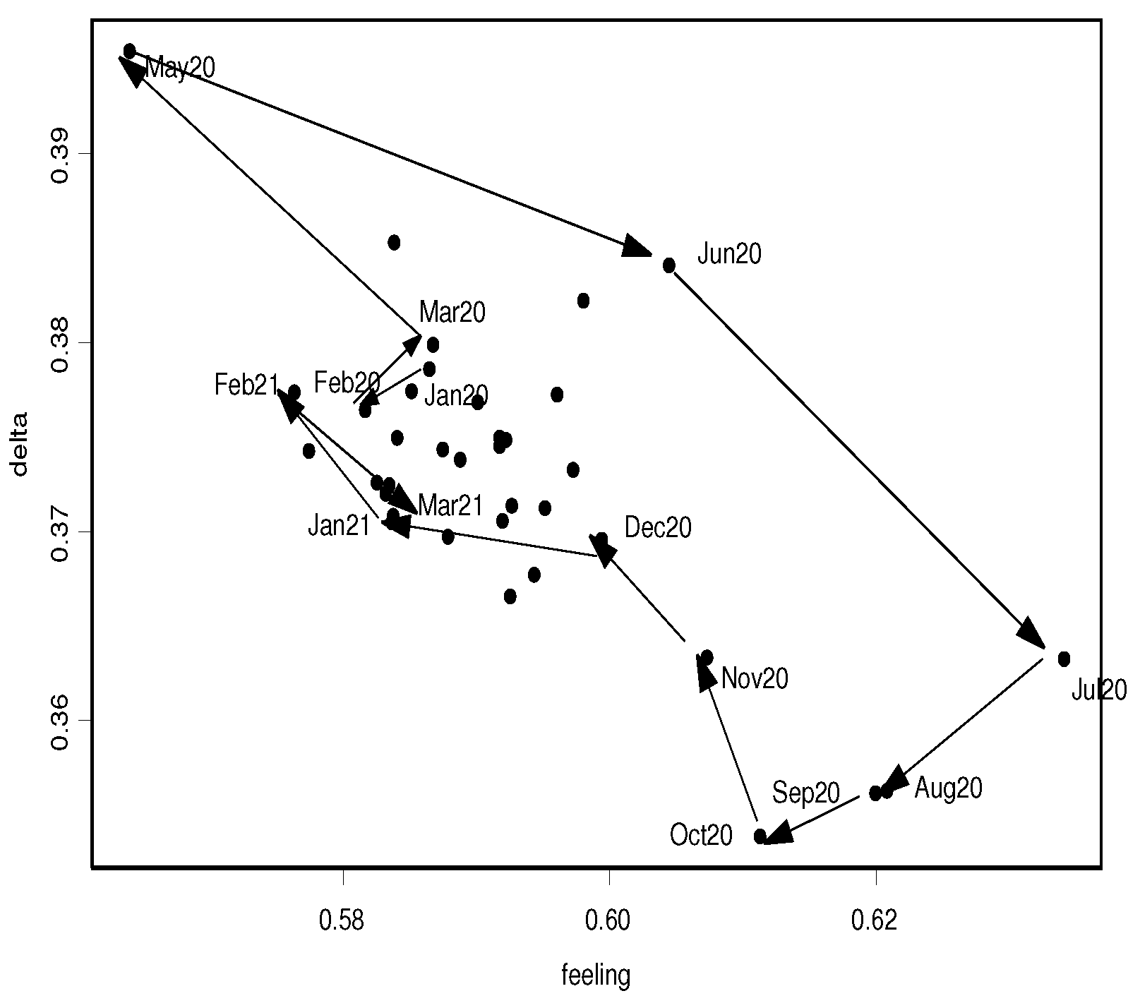
The scatterplots of the estimated uncertainty versus the feeling (left panel of Figure 3), and versus the refuge category coefficient (right panel of Figure 3), show the trajectories that these parameters followed from January 2020 to March 2021. In particular, after the pandemic broke out, moving from March to May 2020 (the lockdown period), consumers’ opinions were better defined (both the uncertainty and the weight of the neutral category decreased) and a greater number of respondents believed that inflation was going to rise (the feeling increased). As mentioned before, consumers based these opinions on a limited and biased set of information about prices.
When the mobility restrictions started to be lifted during the summer, consumers gained a wider view of price developments. The mutual disagreement between opinions increased and the probability that respondents believed that inflation was rising began to decline (the feeling was smaller). At the end of September 2020, the contagion started to spread again, reaching the peak number of Covid cases in November. However, as shown by the trajectories in Figure 3, the parameters followed a path that brought them closer to the bulk of the data. In other words, the initial shock due to the Covid outbreak was completely absorbed.
As regards inflation perceptions, the scatterplot of the uncertainty and refuge components (Figure 4) again showed a path that, from March 2020, moved far from the majority of points. Despite observed inflation declining until the end of 2020, the feeling increased and then the distributions of responses became more left-skewed since a larger proportion of respondents believed that inflation was increasing. Only at the beginning of 2021 did the dynamics of the time-varying parameters return to the pre-Covid pattern.
3.2. The Evolution of Inflation Expectations by Income Group
This section illustrates how the proposed model can be applied to compare opinions given by several groups of respondents.
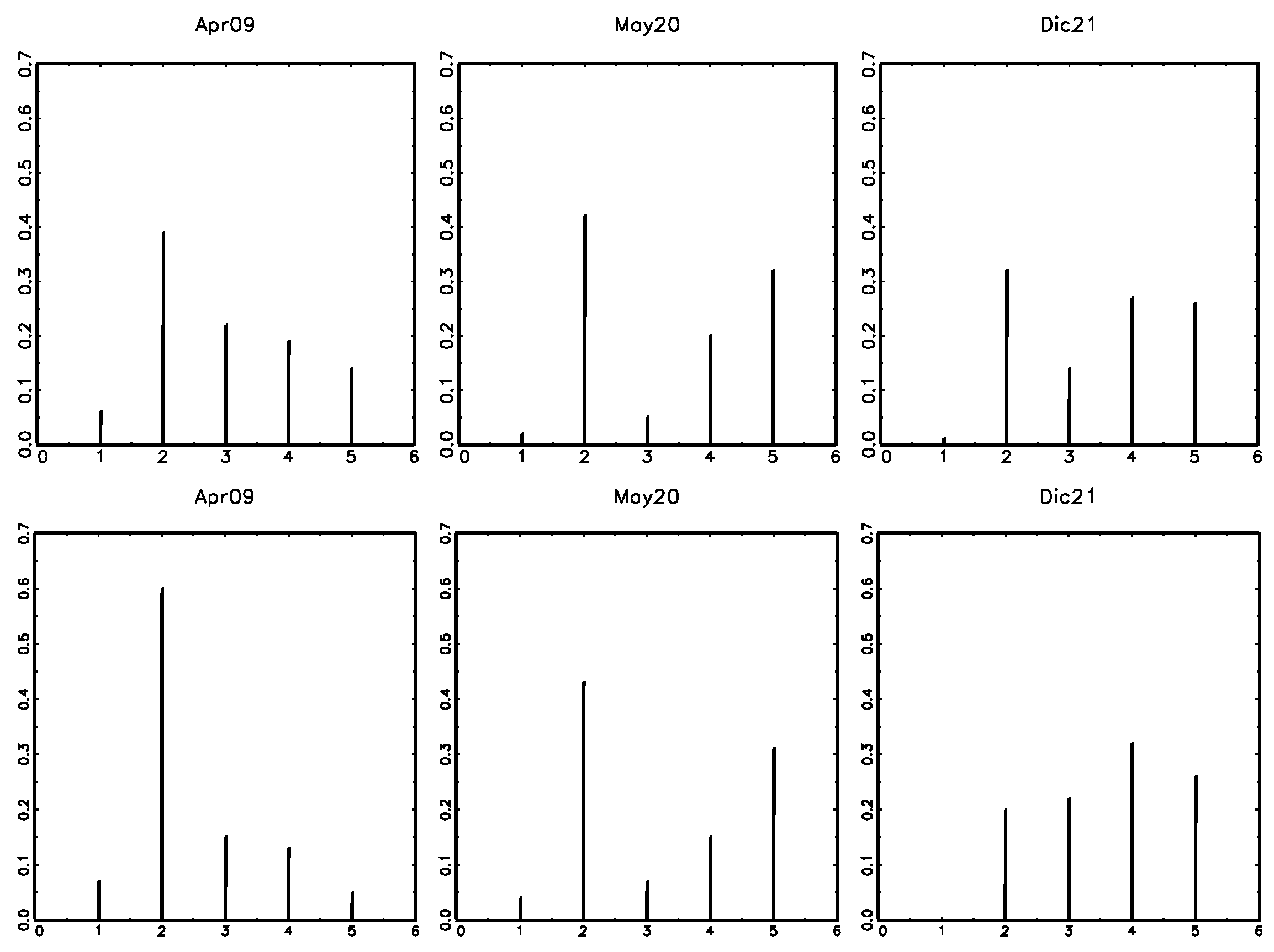
We consider the frequency distributions of the expected direction of change in inflation from January 2006 to July 2022 expressed by consumers classified according to income quartiles (Q1, Q2, Q3 and Q4). Figure 5 exemplifies the frequency distributions of opinions about future inflation of the low-income group (Q1) and the high-income group (Q4) in various instants. The shapes of the distributions of the two groups are rather different and change with time. The presence of the prominent peak at is confirmed.
As discussed in the previous subsection, the model parameters , and depend on aveExp, avePerc, and the difference aveExp−avePerc, respectively. In Table 2, we report the estimated coefficients with the standard errors obtained by 1000 bootstrap replications. The fitting measure, , is satisfactory, in general being above 0.8.
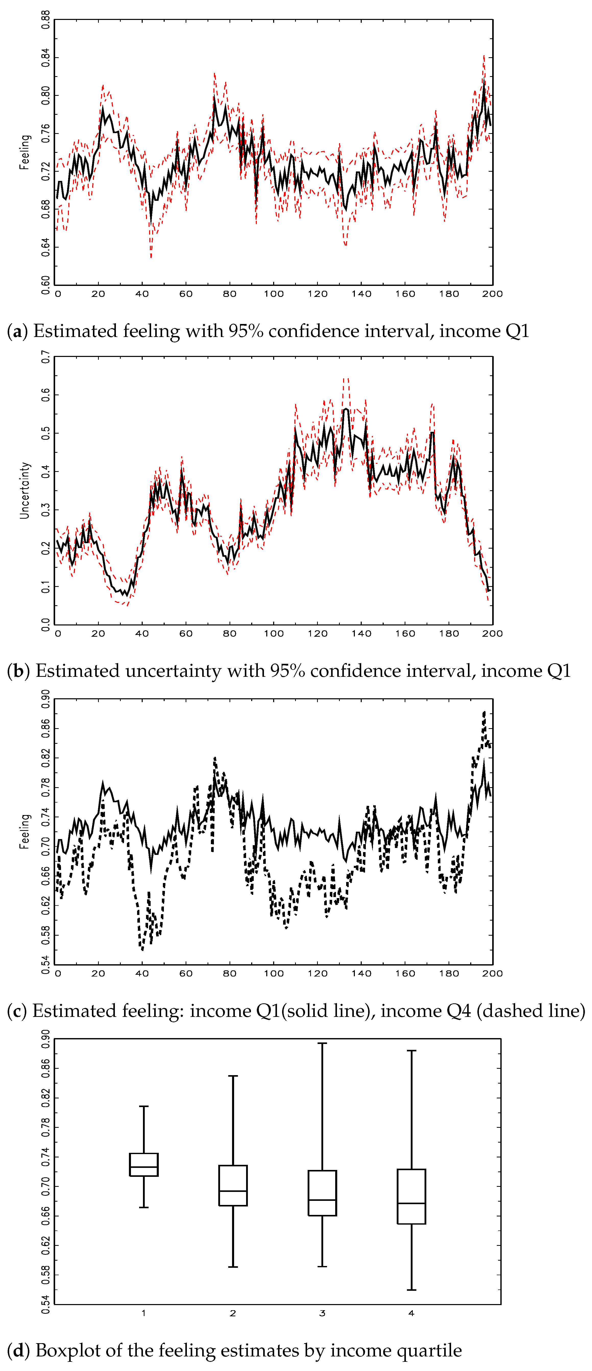
Firstly, we focus on the evolution of the feeling and uncertainty components of the lower income group. The feeling is generally above 0.5, indicating that the distributions are left-skewed; disadvantaged individuals tend to believe that inflation is going to rise in the next year (Figure 6a). The most evident turning points reflect periods when the Italian economic system suffered from significant shocks: the financial crisis between 2007–2009, the sovereign debt crisis at the end of 2011, and the post-pandemic period at the end of 2020. The uncertainty fluctuates over the years, showing higher values during the periods of low/stable inflation and lower values during the crises when opinions tend to concentrate on the extreme of the available rating scale (Figure 6b). The disagreement between respondents changes over time and is considerably influenced by unexpected macroeconomic events.
We now focus on a comparison of the feeling components between low-income and high-income individuals, as illustrated in Figure 6c. For most of the time, the trajectory of the feeling component of low-income earners is higher than that of high-income people. This implies that the distribution of the first group is often more concentrated in rising inflation categories. Disadvantaged people tend to update their expectations more strongly than high-income individuals. This result agrees with the results in [15] obtained from quantitative survey. The possible lower financial literacy and education of disadvantaged people influence the opinion formation about future inflation because the accumulated knowledge about the probable evolution of the phenomenon is limited. Note that, at the end of 2021, the trajectory of the feeling of the high-income group exceeds that of the low-income group. This may be the consequence of the completely new situation caused by the pandemic, which has no reference to past experience and may have severely biased perceptions of the future.
Finally, the behaviour of the remaining two groups is intermediate between the low- and high-income earners. For brevity, we do not report the plots of the corresponding feeling components. The boxplot of the feeling estimates for income groups (Figure 6d) confirms the attitude of low-income respondents of expecting a higher level of inflation in the future, but this attitude tends to decrease as income increases.
4. Discussion
The dynamic CUB model produces an effective description of qualitative data from repeated surveys. In this context, individual data are often not available and information is presented in the form of frequency distributions over time. The model provides a parsimonious parameterization of these distributions. It overcomes the shortcomings related to approaches that rely on separate analysis of the proportions associated with a given category over time, or on the study of the evolution of specific summary statistics, such as the mean of the ordinal distributions.
Two features of the proposed approach are worth noting. Firstly, the parameters of a dynamic CUB model describe a simplified opinion formation mechanism, including the feeling, the uncertainty and the weight of the shelter category. At a given time, these components are affected by the set of information that the respondents have about the economic situation. This set of information can be summarized by a reduced number of explanatory variables that can be used to allow the CUB parameters to vary over time. The pattern of these estimated time-varying parameters is useful for detecting how the pattern of positive/negative opinions changes over time. Secondly, the model provides a characterization of the data-generating process of the opinions of subgroups of respondents. This represents a valuable approach for quantifying the results from qualitative surveys so that differences in the opinions of clusters of respondents can be identified.
Author Contributions
Conceptualization, M.C. and D.P.; methodology, M.C. and D.P.; software, M.C. and D.P.; investigation, M.C. and D.P.; writing—original draft preparation, M.C. and D.P.; writing—review and editing, M.C. and D.P. All authors have read and agreed to the published version of the manuscript.
Funding
This research received no external funding.
Data Availability Statement
Qualitative inflation perceptions and expectations in EU member states (from 1985 onward) can be downloaded from the European Business and Consumer Survey Time-series website at https://ec.europa.eu/info/business-economy-euro/indicators-statistics/economic-databases/business-and-consumer-surveys/download-business-and-consumer-survey-data/time-series_enData (accessed on 1 September 2022).
Acknowledgments
This research was partly presented at the MAF 2022 Conference—Mathematical and Statistical Methods for Actuarial Sciences and Finance held on 20–22 April 2022 at the University of Salerno (Italy).
Conflicts of Interest
The authors declare no conflict of interest.
References
- Mitchell, J.; Smith, R.J.; Weale, M.R. Forecasting manufacturing output growth using firm-level survey data. Manch. Sch. 2005, 73, 479–499. [Google Scholar] [CrossRef]
- Theil, H. On the time shape of economic microvariables and the Munich business test. Int. Stat. Rev. 1952, 20, 105–120. [Google Scholar] [CrossRef]
- Carlson, J.; Parkin, M. Inflation expectations. Economica 1975, 42, 123–138. [Google Scholar] [CrossRef]
- Pesaran, M.H. Expectation formation and macroeconomic modelling. In Contemporary Macroeconomic Modelling; Malgrange, P., Muet, P.A., Eds.; Blackwell: Oxford, UK, 1984; pp. 27–55. [Google Scholar]
- Nardo, M. The quantification of qualitative survey data: A critical assessment. J. Econ. Surv. 2003, 17, 645–668. [Google Scholar] [CrossRef]
- Proietti, T.; Frale, C. New proposals for the quantification of qualitative survey data. J. Forecast. 2011, 30, 393–408. [Google Scholar] [CrossRef] [Green Version]
- Piccolo, D. On the moments of a mixture of uniform and shifted binomial random variables. Quad. Stat. 2003, 5, 85–104. [Google Scholar]
- Piccolo, D.; Simone, R. The class of CUB models: Statistical foundations, inferential issues and empirical evidence, (with discussion and rejoinder). Stat. Meth. Appl. 2019, 28, 389–435. [Google Scholar] [CrossRef]
- Piccolo, D. Observed information matrix for MUB models. Quad. Stat. 2006, 8, 33–78. [Google Scholar]
- Corduas, M.; Iannario, M.; Piccolo, D. A class of statistical models for evaluating services and performances. In Statistical Methods for the Evaluation of Educational Services and Quality of Products; Monari, P., Bini, M., Piccolo, D., Salmaso, L., Eds.; Physica: Heidelberg, Germany, 2009; pp. 99–117. [Google Scholar]
- Piccolo, D.; Simone, R.; Iannario, M. Cumulative and CUB models for rating data: A comparative analysis. Int. Stat. Rev. 2019, 87, 207–236. [Google Scholar] [CrossRef]
- Proietti, T. Discussion of “The class of CUB models: Statistical foundations, inferential issues and empirical evidence”. Stat. Meth. Appl. 2019, 28, 451–456. [Google Scholar] [CrossRef]
- Simone, R.; Piccolo, D.; Corduas, M. Dynamic modelling of price expectations. In CLADAG 2019-Book of Short Papers; Porzio, G.C., Greselin, F., Balzano, S., Eds.; Edizioni Università di Cassino: Cassino, Italy, 2019; Available online: http://cladag2019.unicas.it/book-of-abstracts/ (accessed on 1 September 2022).
- Clar, M.; Duque, J.C.; Moreno, R. Forecasting business and consumer surveys indicators: A time-series models competition. Appl. Econ. 2007, 39, 2565–2580. [Google Scholar] [CrossRef]
- Arioli, R.; Bates, C.; Dieden, H.; Duca, I.; Friz, R.; Gayer, C.; Kenny, G.; Meyler, A.; Pavlova, I. EU Consumers’ Quantitative Inflation Perceptions and Expectations: An Evaluation; EU Economy Discussion Paper, n. 38; European Central Bank: Luxembourg, 2016. [Google Scholar]
- Capecchi, S.; Iannario, M. Gini heterogeneity index for detecting uncertainty in ordinal data surveys. METRON 2016, 74, 223–232. [Google Scholar] [CrossRef]
- Berkson, J. Minimum chi-square, not maximum likelihood! Ann. Stat. 1980, 8, 457–487. [Google Scholar] [CrossRef]
- Harris, R.R.; Kanji, G.K. On the use of minimum chi-square estimation. J. R. Stat. Soc. D 1983, 32, 379–394. [Google Scholar] [CrossRef]
- Cressie, N.; Read, T.R. Multinomial goodness-of-fit tests. J. R. Stat. Soc. B 1984, 46, 440–464. [Google Scholar] [CrossRef]
- Pardo, L. Statistical Inference Based on Divergence Measures; Chapmann & Hall/CRC Press: Boca Raton, FL, USA, 2006. [Google Scholar]
- Rao, C.R. Asymptotic efficiency and limiting information. In Proceedings of the Fourth Berkeley Symposium on Mathematical Statistics and Probability; University of California: Berkeley, CA, USA, 1961; Volume 1, pp. 531–546. [Google Scholar]
- Corduas, M. A dynamic model for ordinal time series: An application to consumers’ perceptions of inflation. In Statistical Learning and Modeling in Data Analysis; Balzano, S., Porzio, G.C., Salvatore, R., Vistocco, D., Vichi, M., Eds.; Springer: Cham, Switzerland, 2019; pp. 37–45. [Google Scholar]
- Efron, B.; Tibshirani, R.J. An Introduction to the Bootstrap; Chapman and Hall: New York, NY, USA, 1993. [Google Scholar]
- Lahiri, S.N. Resampling Methods for Dependent Data; Springer: New York, NY, USA, 2003. [Google Scholar]
- Ranyard, R.; Del Missier, F.; Bonini, N.; Duxbury, D.; Summers, B. Perceptions and expectations of price changes and inflation: A review and conceptual framework. J. Econ. Psychol. 2008, 29, 378–400. [Google Scholar] [CrossRef]
- Corduas, M. Gender differences in the perception of inflation. J. Econ. Psychol. 2022, 90, 102522. [Google Scholar] [CrossRef]
- Simmons, P.; Weiserbs, D. Consumer Price Perceptions and Expectations. Oxf. Econ. Pap. 1992, 44, 35–50. [Google Scholar] [CrossRef]
- Xu, Y.; Chang, H.; Lobonţ, O.; Su, C. Modeling heterogeneous inflation expectations: Empirical evidence from demographic data? Econ. Mod. 2016, 57, 53–163. [Google Scholar] [CrossRef]
- Döhring, B.; Mordonu, A. What Drives Inflation Perceptions? A Dynamic Panel Data Analysis; Economic Papers n. 284; European Commission: Bruxelles, Belgium, 2007.
- Greitemeyer, T.; Schulz-Hardt, S.; Traut-Mattausch, E.; Frey, D. The influence of price trend expectations on price trend perceptions: Why the Euro seems to make life more expensive? J. Econ. Psychol. 2005, 26, 541–548. [Google Scholar] [CrossRef]
- Traut-Mattausch, E.; Schulz-Hardt, S.; Greitemeyer, T.; Frey, D. Expectancy confirmation in spite of disconfirming evidence: The case of price increases due to the introduction of the Euro. Eur. J. Soc. Psychol. 2004, 34, 739–760. [Google Scholar] [CrossRef]
- Biancotti, C.; Rosolia, A.; Veronese, G.; Kirchner, R.; Mouriaux, F. COVID-19 and Official Statistics: A Wakeup Call? Bank of Italy Occasional Paper, n. 605; Banca d’Italia: Rome, Italy, 2021.
- Cavallo, A. Inflation with Covid Consumption Baskets; NBER Working Paper n. 27352. 2020. Available online: http://www.nber.org/papers/w27352 (accessed on 1 September 2022).
- Coleman, W.; Nautz, D. Inflation Expectations, Inflation Target Credibility and the COVID-19 Pandemic: New Evidence from Germany. J. Money Credit Bank 2023. [Google Scholar] [CrossRef]
- Gomes, S.; Iskrev, N.; Pires Ribeiro, P. Euro Area Inflation Expectations during the COVID-19 Pandemic. Banco de Portugal Economic Studies. 2021. Available online: https://www.bportugal.pt/sites/default/files/anexos/pdf-boletim/reev7n3_e_0.pdf (accessed on 1 September 2022).
- Armantier, O.; Kosar, G.; Pomerantz, R.; Skandalis, D.; Smit, K.; Topa, G.; van der Klaauw, W. How economic crises affect inflation belief: Evidence from COVID-19 pandemic. J. Econ. Behav. Organ. 2021, 189, 443–469. [Google Scholar] [CrossRef] [PubMed]
- Binder, C. Coronavirus Fears and Macroeconomic Expectations. Rev. Econ. Stat. 2020, 102, 721–730. [Google Scholar] [CrossRef]
- Bruine de Bruin, W.; Vanderklaauw, W.; Downs, J.S.; Fischhoff, B.; Topa, G.; Armantier, O. Expectations of inflation: The role of demographic variables, expectation formation, and financial literacy. J. Consum. Aff. 2013, 44, 381–402. [Google Scholar] [CrossRef]
- Lü, X.; Hui, H.W.; Liu, F.F.; Bai, Y.L. Stability and optimal control strategies for a novel epidemic model of COVID-19. Nonlinear Dyn. 2021, 106, 1491–1507. [Google Scholar] [CrossRef]
- Yin, M.; Zhu, Q.; Lü, X. Parameter estimation of the incubation period of COVID-19 based on the doubly interval-censored data model. Nonlinear Dyn. 2021, 106, 1347–1358. [Google Scholar] [CrossRef]
- Georganas, S.; Healy, P.J.; Li, N. Frequency bias in consumers’ perceptions of inflation: An experimental study. Eur. Econ. Rev. 2014, 67, 144–158. [Google Scholar] [CrossRef] [Green Version]
- Huber, O.W. Frequency of price increases and perceived inflation: An experimental investigation. J. Econ. Psychol. 2021, 32, 651–661. [Google Scholar] [CrossRef]
- Tversky, A.; Kahneman, D. Availability: A heuristic for judging frequency and probability. Cogn. Psychol. 1973, 5, 207–232. [Google Scholar] [CrossRef]
Figure 1.
Consumer price monthly inflation rate.

Figure 2.
Frequency distributions of inflation expectations (first row) and perceptions (second row) for selected dates.
Figure 2.
Frequency distributions of inflation expectations (first row) and perceptions (second row) for selected dates.

Figure 3.
Inflation expectations: scatterplot of vs. (left panel); vs. (right panel).

Figure 4.
Inflation perceptions: scatter plot of vs. .

Figure 5.
Frequency distributions of expectations about inflation by income quartile: Q1 (first row); Q4 (second row).
Figure 5.
Frequency distributions of expectations about inflation by income quartile: Q1 (first row); Q4 (second row).

Figure 6.
Graphs of time-varying parameters for different income groups.


Table 1.
Estimation results (standard errors in parentheses).
| Model | |||||||
|---|---|---|---|---|---|---|---|
| Perceptions | 1.157 | −0.517 | −0.847 | 0.214 | |||
| (0.019) | (0.006) | (0.010) | (0.008) | ||||
| Expectations | 2.333 | −0.370 | −0.017 | −0.518 | −0.090 | −0.897 | |
| (0.228) | (0.077) | (0.754) | (0.255) | (0.008) | (0.051) |
Table 2.
Estimation results (standard errors in parentheses) by income quartile.
| Model | |||||||
|---|---|---|---|---|---|---|---|
| 1st quartile | −4.267 | 1.479 | 0.481 | −0.487 | −0.367 | 0.435 | |
| (0.674) | (0.194) | (0.423) | (0.122) | (0.054) | (0.095) | ||
| 2nd quartile | −2.622 | 1.038 | 1.692 | −0.859 | −0.352 | 0.469 | |
| (0.392) | (0.251) | (0.829) | (0.251) | (0.055) | (0.087) | ||
| 3rd quartile | −1.831 | 0.852 | 1.987 | −0.953 | −0.310 | 0.334 | |
| (0.817) | (0.255) | (0.385) | (0.124) | (0.059) | (0.101) | ||
| 4th quartile | −2.018 | 0.906 | 2.274 | −1.043 | −0.413 | 0.379 | |
| (0.707) | (0.228) | (0.430) | (0.136) | (0.043) | (0.069) |
Disclaimer/Publisher’s Note: The statements, opinions and data contained in all publications are solely those of the individual author(s) and contributor(s) and not of MDPI and/or the editor(s). MDPI and/or the editor(s) disclaim responsibility for any injury to people or property resulting from any ideas, methods, instructions or products referred to in the content. |
© 2023 by the authors. Licensee MDPI, Basel, Switzerland. This article is an open access article distributed under the terms and conditions of the Creative Commons Attribution (CC BY) license (https://creativecommons.org/licenses/by/4.0/).
Share and Cite
MDPI and ACS Style
Corduas, M.; Piccolo, D. Modelling Qualitative Data from Repeated Surveys. Computation 2023, 11, 64. https://doi.org/10.3390/computation11030064
AMA Style
Corduas M, Piccolo D. Modelling Qualitative Data from Repeated Surveys. Computation. 2023; 11(3):64. https://doi.org/10.3390/computation11030064
Chicago/Turabian StyleCorduas, Marcella, and Domenico Piccolo. 2023. "Modelling Qualitative Data from Repeated Surveys" Computation 11, no. 3: 64. https://doi.org/10.3390/computation11030064
Note that from the first issue of 2016, this journal uses article numbers instead of page numbers. See further details here.