
Performance Investigation for Medical Image Evaluation and Diagnosis Using Machine-Learning and Deep-Learning Techniques

Computer Science Department, University POLITEHNICA of Bucharest, 060042 Bucharest, Romania
*
Author to whom correspondence should be addressed.
Computation 2023, 11(3), 63; https://doi.org/10.3390/computation11030063
Submission received: 17 February 2023
/
Revised: 12 March 2023
/
Accepted: 15 March 2023
/
Published: 20 March 2023
(This article belongs to the Special Issue Computational Medical Image Analysis)
Abstract
:Today, medical image-based diagnosis has advanced significantly in the world. The number of studies being conducted in this field is enormous, and they are producing findings with a significant impact on humanity. The number of databases created in this field is skyrocketing. Examining these data is crucial to find important underlying patterns. Classification is an effective method for identifying these patterns. This work proposes a deep investigation and analysis to evaluate and diagnose medical image data using various classification methods and to critically evaluate these methods’ effectiveness. The classification methods utilized include machine-learning (ML) algorithms like artificial neural networks (ANN), support vector machine (SVM), k-nearest neighbor (KNN), decision tree (DT), random forest (RF), Naïve Bayes (NB), logistic regression (LR), random subspace (RS), fuzzy logic and a convolution neural network (CNN) model of deep learning (DL). We applied these methods to two types of datasets: chest X-ray datasets to classify lung images into normal and abnormal, and melanoma skin cancer dermoscopy datasets to classify skin lesions into benign and malignant. This work aims to present a model that aids in investigating and assessing the effectiveness of ML approaches and DL using CNN in classifying the medical databases and comparing these methods to identify the most robust ones that produce the best performance in diagnosis. Our results have shown that the used classification algorithms have good results in terms of performance measures.
1. Introduction
The world is changing at such a rapid pace that the pressure on healthcare is increasing; adverse changes in climate, environment, and human lifestyle raise the degree of danger, as well as diseases in individuals. This work is focused on analyzing lung diseases and melanoma skin cancer, conditions which, if detected early, can be properly treated. One of the most seriously injured organs is the lung; people can develop a wide variety of lung diseases [1]. Skin cancer is a common type of cancer that affects people with fair skin, and melanoma is a particularly dangerous type of skin cancer; it may quickly transition between different body parts, and has the greatest fatality rate. However, if it is recognized and treated early, the chances of it being cured are higher, necessitating early detection [2].
The traditional methods of diagnosis are costly and time-consuming due to the involvement of trained experts, as well as the requirement of a well-equipped environment. Recent advances in computerized solutions for diagnosis are quite promising, showing increased accuracy and efficiency [3]. By applying medical image-processing techniques to chest X-ray and melanoma skin cancer dermoscopy images, we can assist in detecting diseases earlier and more accurately, which can save many humans. Lung and melanoma skin cancer are two diseases that can be detected earlier and more accurately thanks to the development of technology and computers [4].
Machine-learning and deep-learning techniques have recently attained impressive results in the image-processing field along with medical science. Several areas of healthcare have successfully used machine-learning algorithms [5]. In recent years, various researchers have suggested various artificial intelligence (AI)-based treatments for various medical issues. The DL using the CNN method has enabled researchers to achieve successful outcomes in a variety of medical applications, such as skin cancer classification from skin images and disease prediction from X-ray images. Due to this development, numerous studies have been conducted to determine how DL and ML may affect the healthcare field and medical-imaging diagnostics [6].
ML is the process of teaching a computer to use its prior expertise to solve a problem [7]. Because of the current availability of cheaper processing power and inexpensive memory, the concept of applying ML in several fields to resolve problems more quickly than humans has attracted substantial interest. This allows for the processing and analysis of vast amounts of data to identify insights and correlations within the data that would not be obvious to the human eye. Its intelligent behaviors are based on many algorithms that allow the computer to deliver salient conclusions [8]. In contrast, DL is a branch of ML offering a more advanced approach which allows computers to automatically extract, analyze, and interpret relevant information from raw data by mimicking how people learn and think. DL is a set of neural data-driven approaches based on autonomous feature engineering processes; its accuracy and performance are due to its automatic learning of features from inputs. CNN is regarded as one of the finest image-recognition and -classification models in DL [9].
In this work, we analyze medical images for two sets of medical databases: the first group is chest X-ray images to detect lung diseases and the second group is skin dermoscopy images to detect melanoma skin cancer. We focus on the use of the most common machine-learning techniques and convolutional neural networks for deep learning to classify the lungs in the first medical dataset into normal and abnormal, and skin lesions in the second medical dataset into malignant and benign to prove the efficiency and effectiveness of these methods in classification and medical diagnosis.
The major goal of this work is to investigate and assess the effectiveness of ML approaches and CNN for the classification of medical databases and compare these methods to identify the methods that have the best performance in diagnosis. We applied these methods to two different types of medical databases to diagnose two different diseases that are considered among the most dangerous, which threaten human life and can be treated if diagnosed early.
The paper is organized as follows: Section 2 presents the current advances in this research field, emphasizing our research in this context. Section 3 explains the components of the proposed system to diagnose lung diseases and melanoma skin cancer. Section 4 presents the chest X-ray and melanoma skin cancer dermoscopy image analysis in detail, as well as the databases resources. Here, the analysis methods are discussed, preprocessing and segmentation methods are presented, and the extraction-of-features methods are introduced, emphasizing the classification techniques employed for lung illness and melanoma skin cancer diagnosis and performance metrics. Section 5 introduces the performance of the results and the comparison between the two datasets. Section 6 provides the most important work contributions. Section 7 discusses the work results and future works. The paper concludes by drawing some conclusions.
2. Related Work
In recent years, several studies have been conducted on performance research for medical image evaluation and diagnosis using ML and DL techniques. In this research field, we did not find any research that incorporates most of the machine-learning methods (as we used) and makes a parallel comparison when using more than one medical database (we used two databases) to assess the effectiveness of ML and DL methods. The authors of [10] evaluated the SVM and RF machine-learning techniques, as well as CNN for detecting breast cancer in thermographic images; the images were preprocessed to improve them and then isolate the region of interest (ROI). The object-oriented image-segmentation method was used, which eliminated the salt-and-pepper noise from the image and increased its precision using spectral signatures. The forms of the items’ border, thickness, and color of images were extracted as features. Classification algorithms were utilized and evaluated using a variety of metrics, such as validation accuracy, elapsed time, training error, and training precision. In terms of accuracy, precision, and the amount of data needed, CNN outperformed the SVM and RF approaches.
In [11], the effectiveness of deep learning and machine learning was assessed using skin cancer datasets. The proposed method used Laplacian and average filters to eliminate noise from images and dull-razor techniques to remove hair. For image segmentation, the region-growth method was used. Three techniques were utilized to extract hybrid features: GLCM, discrete wavelet transform (DWT), and local binary pattern (LBP). These features were then combined into a feature vector and categorized utilizing ANN and feed-forward neural network (FFNN) classifiers of machine-learning methods and CNN models (ResNet-50 and AlexNet). The approaches were evaluated using statistical measures (accuracy, precision, sensitivity, specificity, and AUC), where the FFNN and ANN classifiers outperformed the CNN models. The authors of [12] developed a system for predicting lung diseases such as pneumonia and COVID-19 from patients’ chest X-ray images; they used median filtering and histogram equalization to improve the image quality. They developed a modified region-growing technique for extracting the ROI of the chest areas. They extracted a set of features represented by texture, shape, visual, and intensity features followed by normalization. ANN, SVM, KNN, ensemble classifiers, and deep-learning classifiers were utilized for classification. Deep-learning architecture based on recurrent neural networks (RNN) with long short-term memory was suggested for the accurate identification of lung illnesses (LSTM). The approaches were evaluated using metric measures (accuracy, specificity, precision, recall, and F-measure). The F-RNN-LSTM approach had the highest accuracy.
In [13], the findings and analysis of the UCI Heart Disease dataset were compared using various machine-learning and deep-learning methodologies. The dataset contained 14 major attributes which were used in the study. Several promising results were achieved and validated using accuracy, sensitivity, and specificity. Isolation forest was used to address certain uninteresting aspects of the dataset. Deep learning achieved higher accuracy compared with the ML methods that were used in the work. The authors of [14] created a model that aided in the diagnosis of chest X-ray medical images and classified the images into healthy and sick by employing six machine-learning techniques (DT, RF, KNN, AdaBoost, Gradient Boost, XGBboost) and a CNN model to improve efficiency and accuracy. The approach begins by reducing the size of chest X-ray images before identifying and classifying them using the conventional neural network framework, which extracts and classifies information from the images. The model’s performance was estimated utilizing classification accuracy and cross-validation. Deep learning had the highest accuracy. The decision tree classifier, on the other hand, had the lowest performance.
The authors of [15] investigated the efficiency of various ML and DL algorithms for detecting Plasmodium on digital microscopy cell pictures. They used a publicly available dataset that included equal numbers of parasitized and uninfected cells. They used color constancy and spatially resampled all images to a specific size based on the classification architecture used, and they presented a swift CNN architecture. Additionally, they investigated and evaluated the effectiveness of transfer-learning algorithms built on well-known network topologies such as AlexNet, ResNet, VGG-16, and DenseNet. They also studied how well the bag-of-features model performed when used with an SVM for classification. Based on the average probabilities provided by all the developed CNN architectures, the probability of a cell image containing Plasmodium was calculated. All deep-learning- and transfer-learning-based techniques outperformed the bag-of-features and SVM-based classification models.
In comparison with previous studies, we noticed the following:
- The proposed system in this work dealt with two different types of databases for evaluating two different diseases and determining the performance of DL and ML methods, while all previous studies dealt with one database for diagnosing one type of disease for evaluating the performance of DL and ML methods. A continuous comparison between the application of the methods on both datasets has been made, emphasizing the fact that the type of evaluated disease matters.
- In comparison with [11], we note that the authors used a dull-razor tool to remove hair from skin images, while we suggested in our work an accurate algorithm to remove hair from skin images while preserving the shape of the lesion and the quality of the image.
- We noticed that most of the previous studies [10,11,12] used the object-oriented image method in the segmentation stage to extract the ROI from the images. In our study, we proposed methods for extracting the ROI (lung and skin lesions) that depend on the threshold techniques, binarization, negation, and morphological operations to segment the colored and gray level images. In addition to this, ref. [14] does not mention any image-segmentation method.
- Compared with previous studies, our study focused on extracting hybrid features from images, which included most types of features (texture, color, shape, geometry, and intensity), and different methods for extracting features were addressed.
- In the classification stage, we noticed that our study dealt with most of the methods of machine learning (nine methods) for an advanced comparison, while the rest of the studies dealt with a limited number of machine-learning methods, and may be limited to one [15], two [10,11], or three methods [12].
We concluded from the comparison that our work was more comprehensive and more in-depth in evaluating the performance of machine-learning and deep-learning methods in diagnosing diseases, and it provided good results in addition to offering a better overview of the ML methods. In this way, our work can be considered a good start for any researcher that has to choose an appropriate technique.
3. Workflow Design
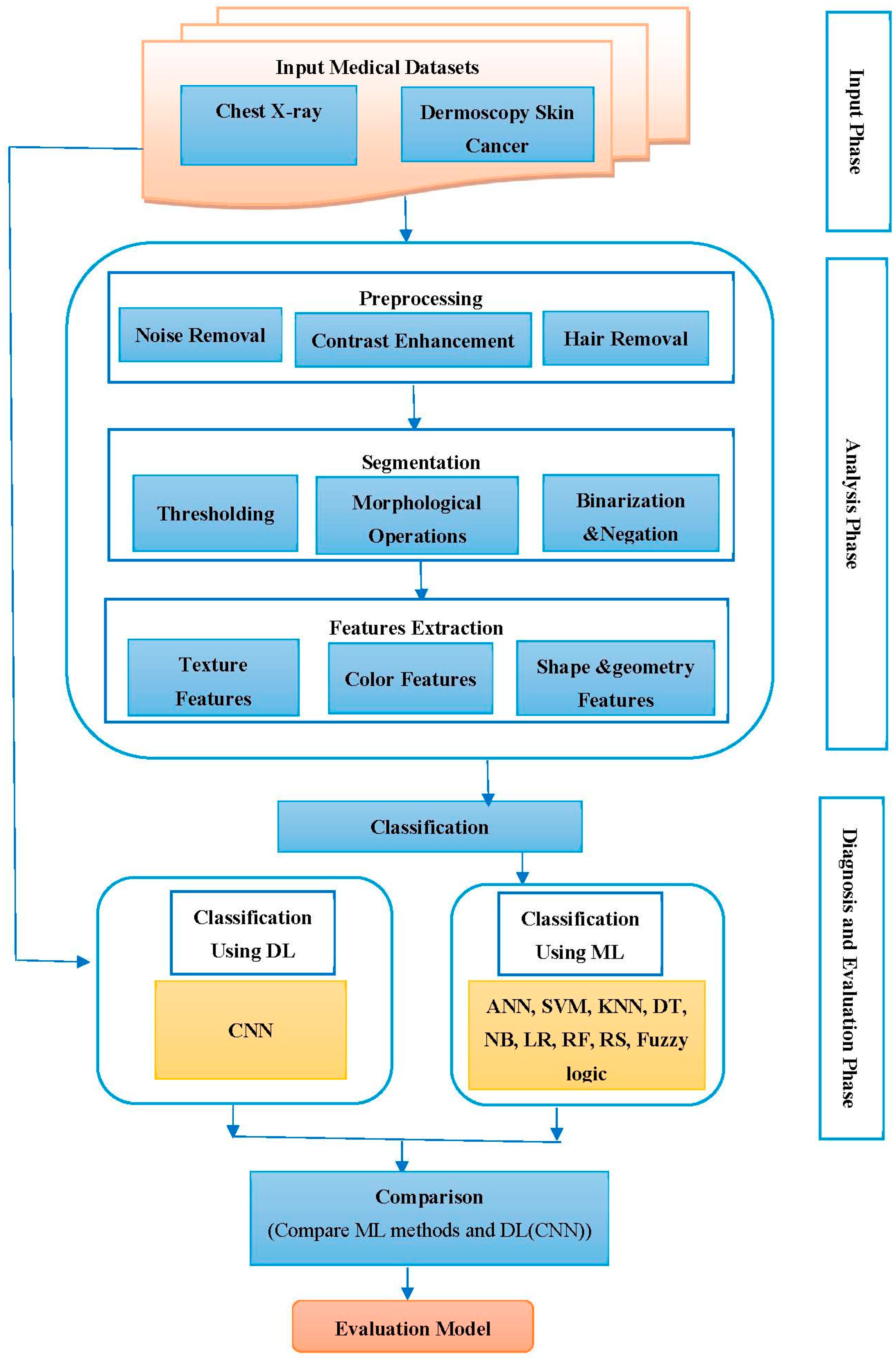
This section describes the proposed framework, which is divided into three phases: the first phase is responsible for acquiring medical datasets to be analyzed in the next phase; the second phase is responsible for analyzing the input medical dataset that includes preprocessing medical images to improve them, extracting the region of interest (ROI), and then extracting significant features that help in classification. The third phase is responsible for the diagnosis and evaluation, where selected classification methods are applied to the selected datasets, and then these methods are evaluated. All the algorithms and processes of the proposed work were implemented using Matlab 2021. Figure 1 shows the whole workflow for the proposed framework.
4. Methods
This section is divided into three parts. The first part deals with the medical datasets used in this work. The second part deals with the analysis of the medical datasets, which involves the stages of preprocessing, segmentation, and feature extraction. The third part deals with the diagnosis and evaluation phase, which involves applying classification algorithms on the selected medical datasets and then evaluating these algorithms.
4.1. Medical Datasets
In this work, we used two sets of medical databases; the first group included images of chest X-rays, and the second group included dermoscopy images for melanoma skin cancer. These databases were divided into 70% for the training and 30% for the testing.
4.1.1. The Chest X-ray Dataset
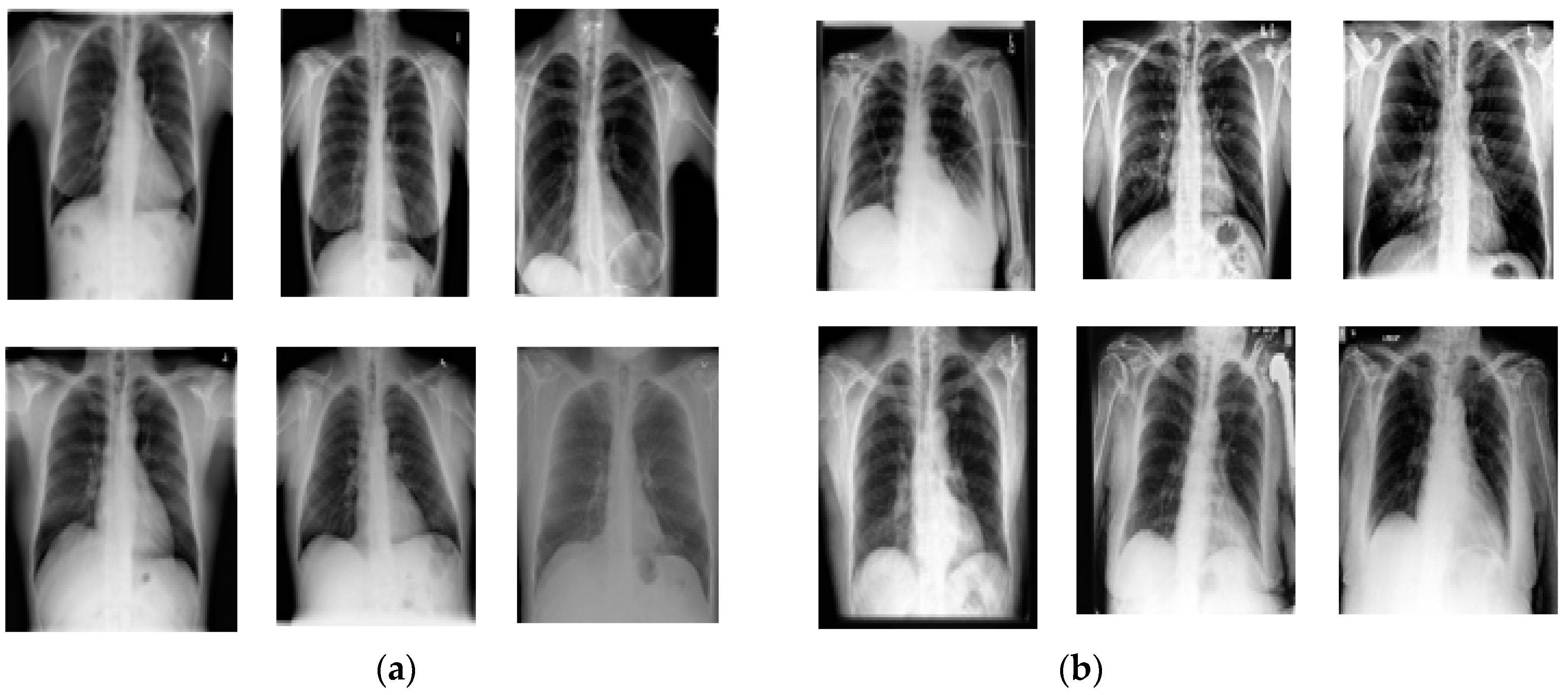
The chest X-ray samples of normal and abnormal lung cases were obtained from Kaggle [16]. A dataset containing 612 images was used for the proposed methodology; among the total 612 images of lungs that were certified in this work, 288 images showed healthy lungs and 324 were images of lungs affected by different types of lung diseases like atelectasis, pneumonia, emphysema, fibrosis, lung opacity, COVID-19, and bacterial and viral diseases. Images were captured in the JPG format, with various resolution sizes; the sizes were standardized to 256 × 256 pixels. Figure 2 illustrates normal and abnormal lung images from the chest X-ray database.
4.1.2. The Dermoscopy Melanoma Skin Cancer Dataset
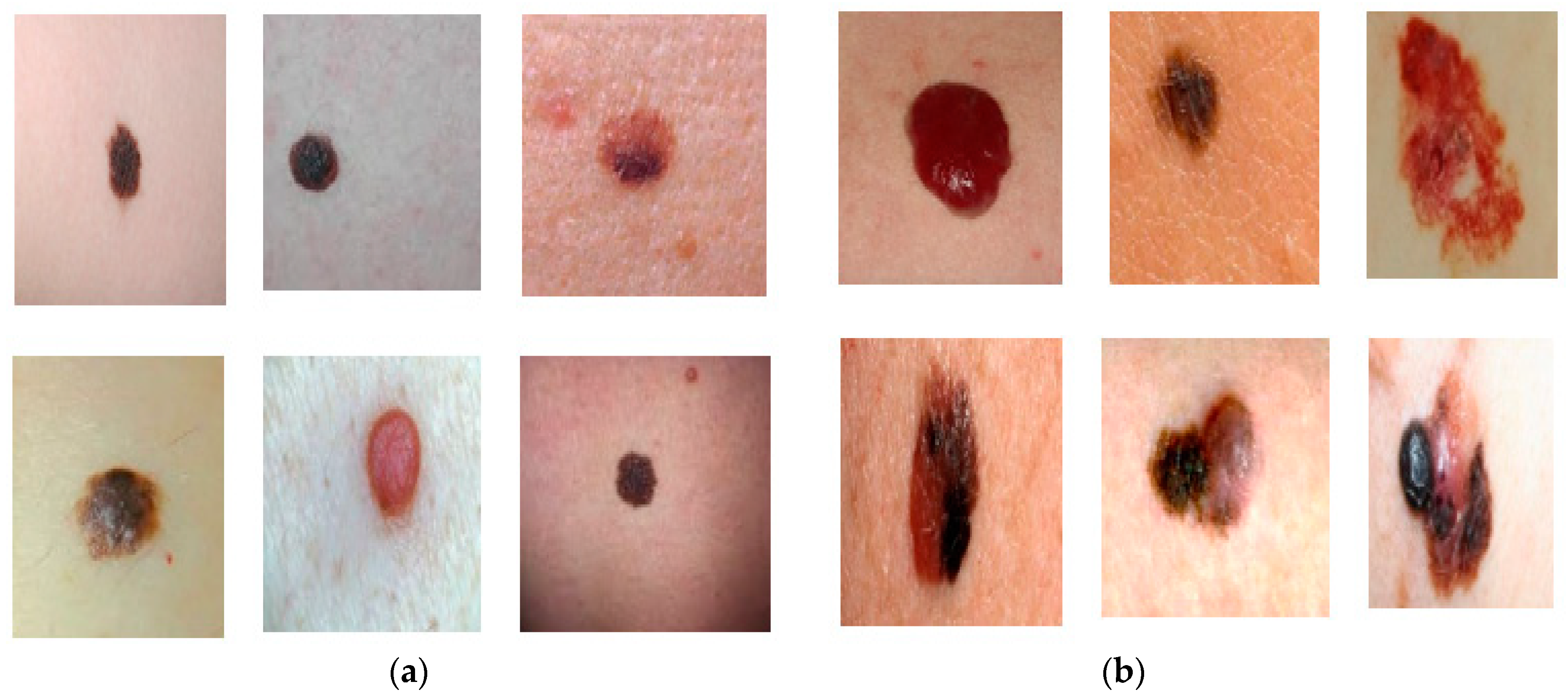
The dermoscopy samples of melanoma skin cancer were obtained from The Lloyd Dermatology and Laser Center [17], and the Dermatology Online Atlas [18]. A dataset containing 300 images was used to evaluate the proposed methodology; among the total of 300 images of melanoma skin cancer which were used in this work, 145 images represented benign conditions and 155 represented malignant ones, which include several types of malignant melanoma-like superficial spreading, nodular, lentigo, and acral malignant melanoma. The images were captured in the JPG format, as in the previous case, and the sizes were standardized to 256 × 256 pixels to extract accurate features that distinguish between benign and malignant melanoma skin cancer images. Figure 3 illustrates benign and malignant images from the melanoma skin cancer dermoscopy database.
4.2. Datasets Analysis
In this section, we discuss the data analysis phase according to the suggested model (shown in Figure 1) employed in the study. This phase contains three stages: preprocessing, segmentation, and feature extraction.
4.2.1. Image Preprocessing
Preprocessing aims to enhance images and remove undesirable effects. Because the quality of the first medical dataset, which contains chest X-ray images, is low and contains noise, the suppression of lung regions affected by congestion or fluids may occur, and the X-ray scan also generates noise in the image. The suggested model for preprocessing the chest X-ray images involves applying three main processes: image cropping, noise removal, and contrast enhancement.
4.2.1.1. Image Cropping
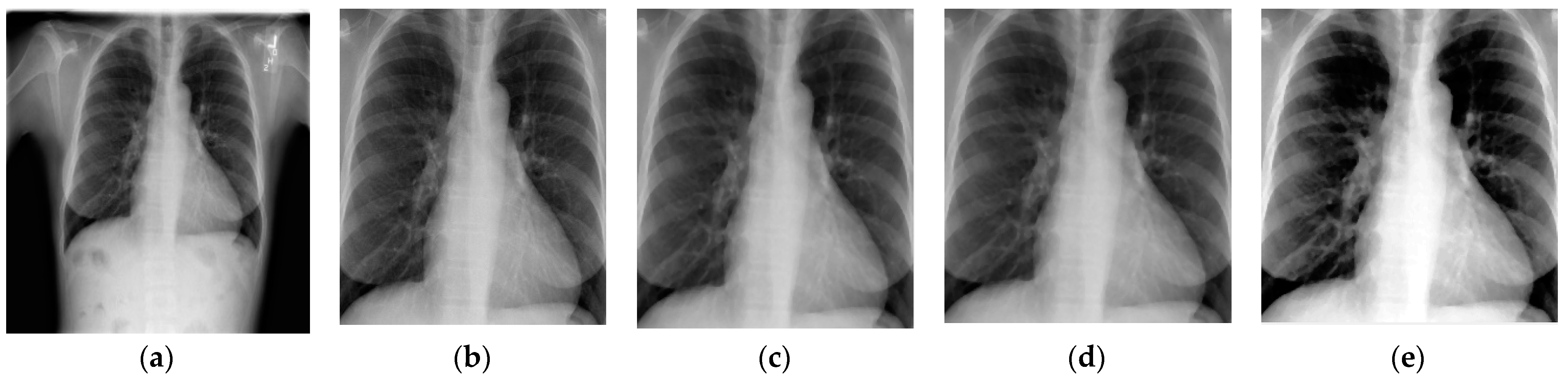
Cropping is applied to the input original chest X-ray images to accentuate the ROI (lung) and remove all undesired artifacts. Image cropping is required to accelerate image processing. Manual cropping is used in this work, where the image is cropped into a square form consisting of the lung, as shown in Figure 4b.
4.2.1.2. Noise Removal
In the case of X-ray datasets, median filtering outperforms adaptive bilateral filtering, average filtering, and Wiener filtering [19]. Median filtering is a simple approach widely utilized in many image-processing applications because it is more successful in noise reduction and edge preservation and eliminates any additional noise present in the image [12]. In the proposed model, we used median filtering, which works by traversing across the image pixel by pixel and replacing every value with the median value of the adjacent pixel. The design of the neighbor is determined by the size of the window; a window size of a 3 × 3 neighborhood was utilized in this work. Figure 4c demonstrates the application of median filtering in a chest X-ray image.
4.2.1.3. Contrast Enhancement
In this process, we utilized the adaptive intensity values adjustment, which concentrates on adjusting the image intensity values for low-contrast X-ray images. In this way, the contrast is improved. Then, we applied histogram equalization for increased contrast to make the ROI clear. The histogram represents the distribution of image pixels; it is calculated by counting the number of times each pixel value appears, and is then mapped against the grayscale image’s intensity [20]. Enhancing the contrast of an image can sharpen its border and increase segmentation accuracy because it creates a contrast between the object and the background. The applied contrast-enhancement process is shown in Figure 4d,e.
The result after applying the main processes of image preprocessing on an example of a chest X-ray image is shown in Figure 4.
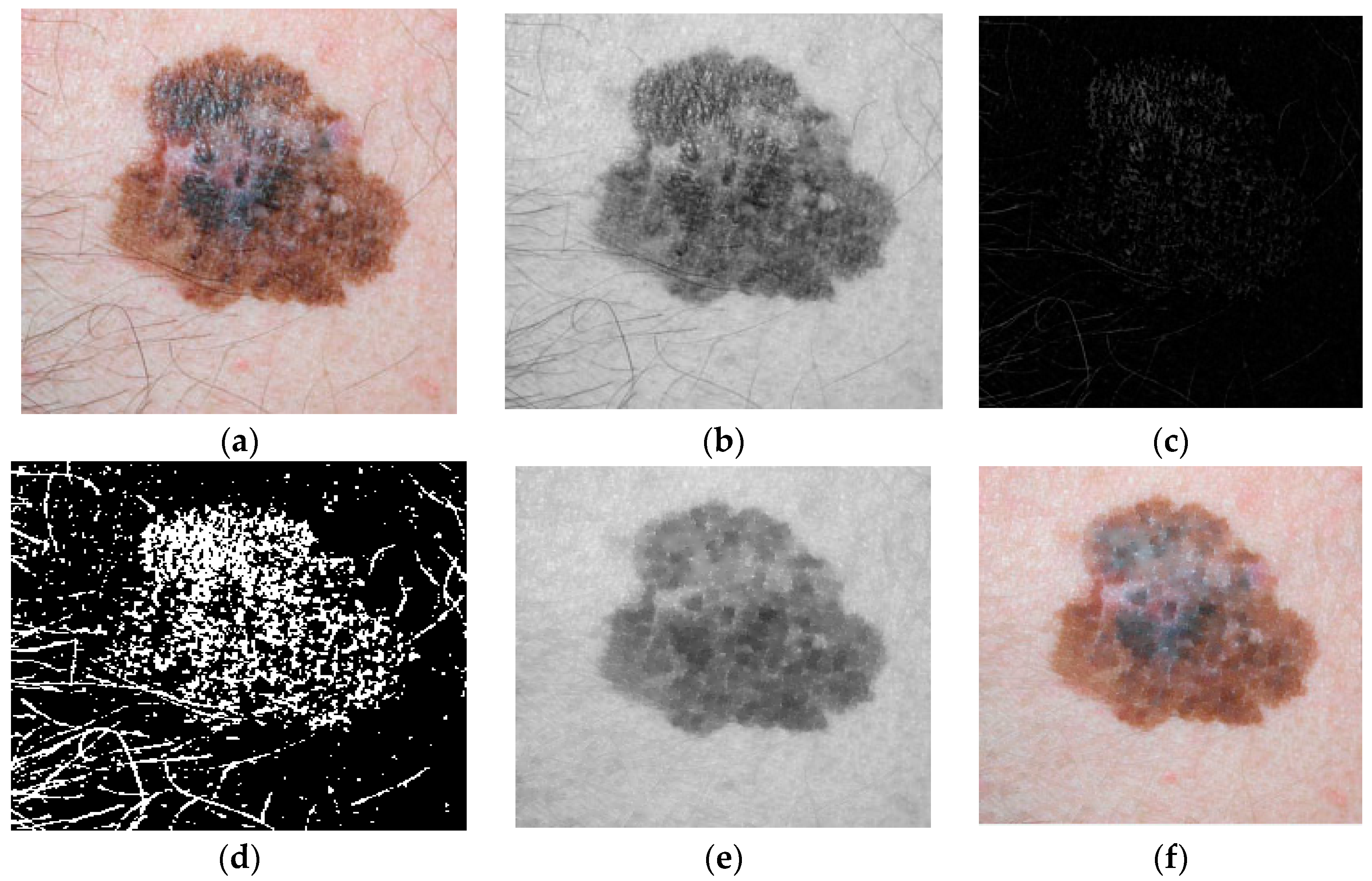
Image preprocessing for the second group, which contains melanoma skin cancer dermoscopy images, involves presenting an algorithm for hair detection and removal. Some of the images of skin may contain hair, and this hair offers an inaccurate classification; as a result, it is preferable to remove the hair before moving on to the next stages. The proposed algorithm creates a clean dermoscopy image while maintaining the dermoscopy appearance by replacing the portions of the image containing hair structures with the neighboring pixels. The original RGB (red, green, blue) dermoscopy image is first transformed into a grayscale image, and then the resulting grayscale image is subjected to a morphological filter known as black top-hat [21,22].
The top-hat morphological filter fills in the image’s minute gaps while preserving the original area sizes; thus, all background areas are removed for the pixel values that act as structuring elements. A thresholding technique is applied to the output of the used top-hat morphological filter to create a binary mask of the undesirable structures present on the dermoscopy image. After the creation of the binary mask of the hair structures, we replace the mask’s pixels to remove undesired pixels while retaining the image’s shape and extracting and restoring the clean skin lesion image [23]. The following four steps describe the hair-removal algorithm:
- The color image is converted into a grayscale image;
- Black top-hat transformation is utilized for the detection of dark and thick hairs and is represented as the following equation:where ● denotes the closing operation, is the local contrasted image, and b is a grayscale structuring element.
- By filling the regions in the image that the mask specifies, we can use region fill to remove items from the image or to replace invalid pixel values with their neighbors. The mask’s nonzero pixels specify the image pixels to be filled.
- The result is a fully preprocessed image maintained throughout the subsequent phases.
Figure 5 shows an example of applying steps of a hair-removal algorithm on a melanoma skin cancer image.
4.2.2. Image Segmentation
Image segmentation is the process of separating an object from an image according to criteria like the gray level of a pixel and the gray level of its nearby pixels. One approach for segmenting is the thresholding method, which divides the grayscale image into segments based on many classes according to the gray level [20]. In this work, image segmentation for the first group containing chest X-ray images involves applying thresholding and morphological operations to the preprocessed image to separate the ROI (lung) from the image. Here, global thresholding was utilized because the intensity distribution between the background and foreground of the image was considerably different. After that, we applied morphological operations, which are a large set of image-processing operations that process medical images according to shapes and facilitate object segmentation from images [24]. In the proposed algorithm, the fill operation was used, which smooths the contour and closes small holes as the inner lining of the shapes fills inward; the restoring fill skips the closed holes, thus making this operation effective for closing holes. Thus, morphological operation helps smooth and simplify the borders of objects without changing their size and improves the specific region for accurate segmentation. Figure 6 shows the steps of the suggested segmentation algorithm for chest X-ray images.
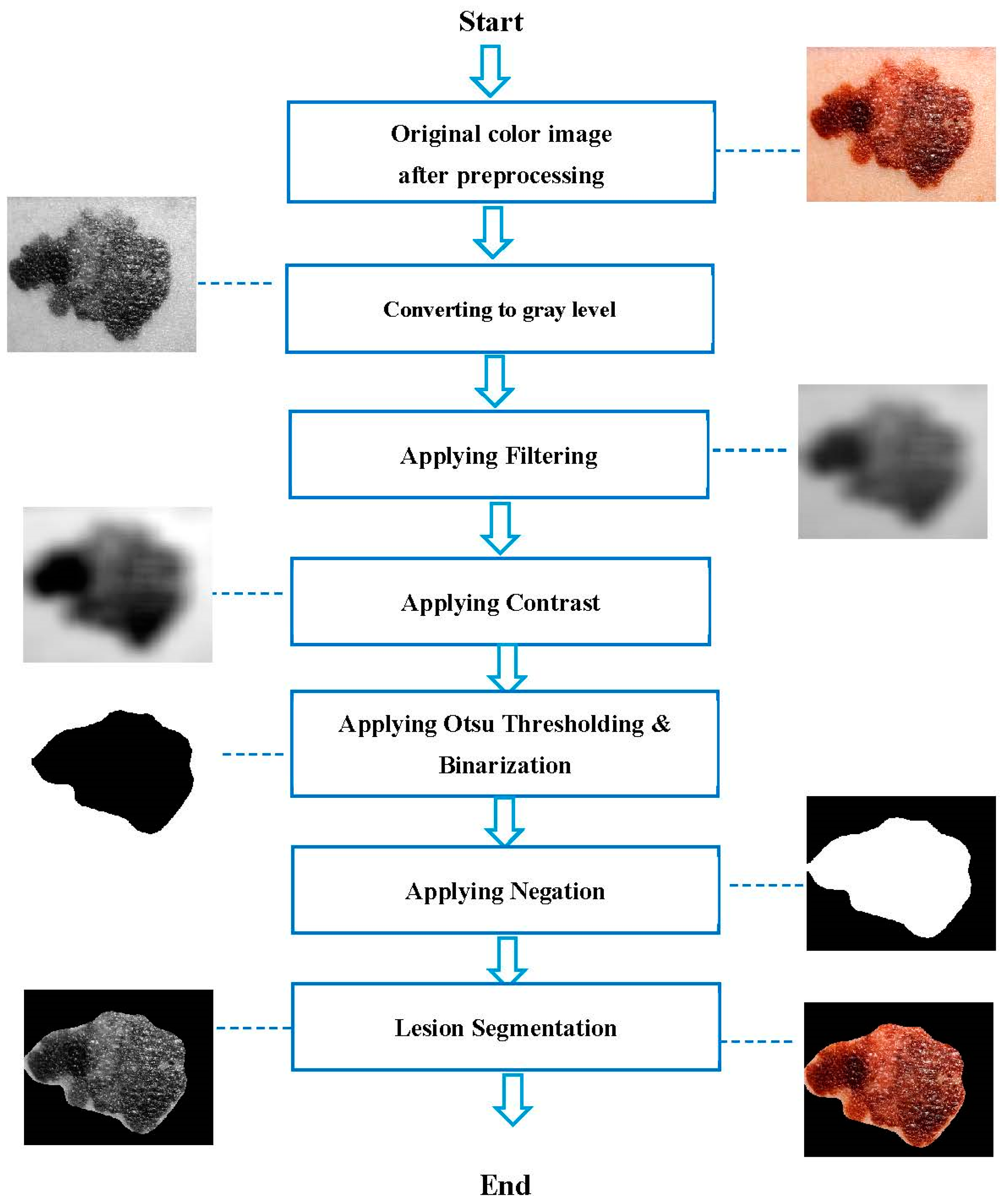
Image segmentation for the second group, which contains melanoma skin cancer dermoscopy images, involves applying Otsu thresholding, binarization, and image negation to the preprocessed image to separate the object (skin lesion) from the image. Here, Otsu thresholding was utilized, which is a thresholding approach that automatically finds the threshold point that splits the gray-level image histogram into two distinct sections. The image’s gray level is expressed as I to L, where I is 0 pixels and L is 255 pixels. The Otsu approach was utilized to automatically determine the threshold according to the input images [20]. Following that, the processes of binarization and image negation were carried out. Binarization via thresholding is the process of converting a grayscale image to a binary image; here, every pixel in the improved image’s gray-level value was computed, and if the value was larger than the global threshold, the pixel value was set to one; otherwise, was is set to zero [25]. During the image negation, an image with white pixels is replaced with black pixels. Meanwhile, white pixels replace dark pixels [20]. After applying the binary mask, the mask is then multiplied by the three color channels (red, green, and blue) to extract the region of interest. Figure 7 shows the steps of the suggested segmentation algorithm for melanoma skin cancer images.
4.2.3. Feature Extraction
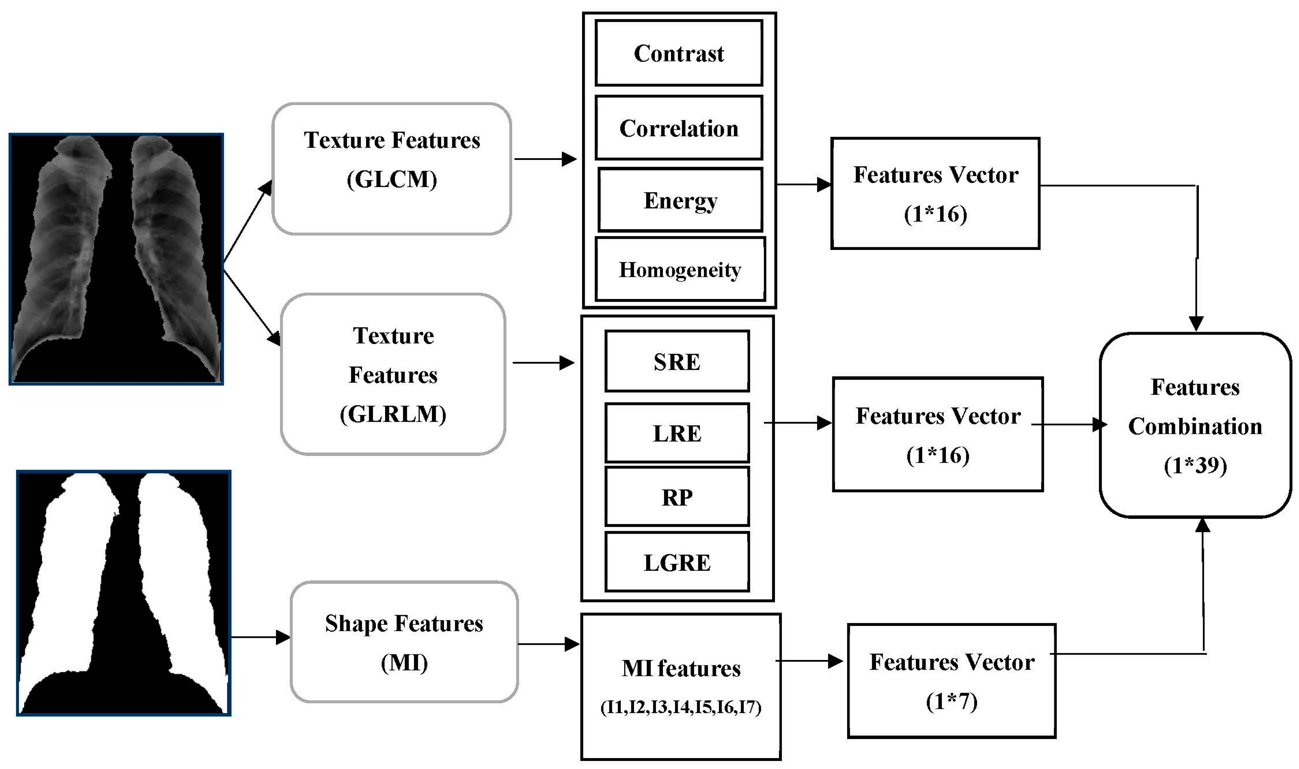
In the feature-extraction stage, we extracted a set of features from images that represent meaningful information fundamental for classification and diagnosis. Several methods are utilized for extracting features such as texture, shape, color, etc. In this work, the color, texture, shape, and geometry features were extracted. To detect normal and abnormal lungs for the first medical dataset (chest X-ray), we combined two types of features, the texture and shape features. The texture features were extracted from the lung in a gray-level image and represented by computing contrast, correlation, energy, and homogeneity from the Gray-Level Co-Occurrence Matrix (GLCM) in four directions (0, 45, 90, and 135), in addition to computing Short-Run Emphasis (SRE), Long-Run Emphasis (LRE), Run Percentage (RP), Low Gray-level Run Emphasis (LGRE) from the Gray-Level Run-Length Matrix (GLRLM) in four directions (0, 45, 90, and 135), and the shape features represented by seven features for moment invariants (MI). Thus, we obtained 16 features from the GLCM method, 16 features from the GLRLM method for texture features, and 7 features from the MI method for shape features. These features were been combined to create a single feature descriptor with 39 features to achieve an accurate output for good classification. Figure 8 shows the extracted features from the lung images in the first medical database.
- A.
- Texture features set
To extract texture features from lung images in the gray level, two suitable methods were used:
- 1.
- Gray-Level Co-occurrence Matrix (GLCM)
GLCM is a well-known statistical method for obtaining texture information from gray-level images [26]. It is the representation of the spatial distribution and the interdependence of the gray levels within a local area. The location of a very gray-level pixel can be found by the GLCM method [27].
Let Ng be the total number of gray levels, g(i,j) be the entry (i,j) in the GLCM, µ be the mean of the GLCM, and σ2 be the variance of the GLCM. Table 1 shows the GLCM features with descriptions and equations.
- 2.
- Gray-Level Run-Length Matrix (GLRLM)
GLRLM is a type of two-dimensional (2D) histogram-like matrix that records the occurrence of all conceivable gray-level values and gray-level run combinations in an ROI for a given direction. Gray-level values and runs are generally denoted as row and column keys in the matrix; hence, the (i,j)-th entry in the matrix identifies the number of pairings whose gray-level value is i and whose run length is j [28,29].
Let P denote a GLRLM, then, Pij is the (i, j)-th entry of the GLRLM, Nr denotes the set of various run lengths, Ng is the set of various gray levels, Np is the number of voxels in the image, and lastly, N represents the number of total pixels. Table 2 shows the GLRLM features with descriptions and equations.
- B.
- Shape features set
MI is characteristic of connected regions in binary images which are invariant to translation, rotation, and scaling. The moments can be used to illustrate the shape of objects. Invariance recognizes the multidimensional moment-invariant-features space. The seven shape attributes are derived from the central moments and are not affected by the object scale, orientation, or translation. The translation of invariant moments at the origins of the central moments is calculated using the center of gravity [30].
The moments are represented by the image of the i j plane with nonzero elements. For a 2D ROI image, the moment invariance of order (p, q) is calculated as [12]:
Lower-order geometric moments have intuitive meaning: m00 is the ROI’s “mass,” and m10/m00 and m01/m00 determine the ROI image’s centroid. In the case of moments invariance, we have central moments of order (p, q) [31]:
where i = m10/m00 and j = m01/m00 are the coordinates of the object centroid. In this way, we calculated seven moments as outlined in Table 3; this table shows the MI features with equations.
To detect benign and malignant skin lesions in melanoma skin cancer images for the second medical dataset (melanoma skin cancer dermoscopy), we combined three kinds of features: color, texture, and geometry features.
The color features were extracted from the skin lesion in color images in the HSV (hue, saturation, value) system, represented by computing the mean, the standard deviation (STD), and skewness for each H, S, and V channel by applying the color-moments (CM) method. The texture features were extracted from the skin lesion in a gray-level image and represented by computing coarseness, contrast, and directionality by applying the Tamura method. The geometry features were extracted from the skin lesion in binary images, represented by computing area, perimeter, diameter, and eccentricity. Thus, we obtained nine features from the CM method for color features, three features from the Tamura method for texture features, and four shape features. These features were combined to create a single feature descriptor with 16 features to achieve an accurate output for good classification. Figure 9 shows the extracted features from the skin lesion for the second medical database images.
- 1.
- Color features set
CMs are one of the simplest and most active features compared with other color features; the features of common moments are mean, standard deviation, and skewness [32].
Let be the color value of the i-th color component of the j-th image pixel and N be the image’s total number of pixels. ,, (i = 1,2,3) represent the mean, standard deviation, and skewness of every channel of an image, respectively. Table 4 shows the CM features with equations.
- 2.
- Texture features set
Tamura is a method for devising texture features based on human visual perception. It identified six textural features (coarseness, contrast, directionality, regularity, roughness, and line-likeness). The first three are very effective outcomes [33,34]. Let n denote the image size, k be the value that maximizes the differences in the moving averages, represent the fourth moment of the image, represent the image standard deviation, denote the local direction histogram, be the peak number of , be the p-th peak position of , be the p-th peak range between valleys, r be a normalizing factor, and be the quantized direction code. Table 5 shows the Tamura features with descriptions and equations.
- 3.
- Geometry features set
The geometry features extracted from a skin lesion in binary images are represented by computing the lesion area, lesion perimeter, eccentricity, and diameter of the lesion. Variable “A” is the lesion area and is a segmented image of x rows and y columns, , , , and , are endpoints on the major axis,,…., is a boundary list, and di is the distance [35]. Table 6 shows the geometry features with descriptions and equations.
4.3. Diagnosis and Evaluation
In this section, we discuss the diagnosis and evaluation phase according to the suggested model (shown in Figure 1) employed in the study.
4.3.1. Classification
Classification is the most significant part of the diagnosis of the medical databases. In this work, we used most of the known ML algorithms such as ANN, SVM, KNN, DT, RF, NB, LR, RS, and fuzzy logic to classify the lungs as normal or abnormal in the first database and the skin lesions as benign or malignant in the second database. Most of these algorithms performed well. In contrast, CNN is regarded as one of the finest image-recognition and classification models in DL [36]. As a result, we used the CNN model to classify the chest X-ray and melanoma skin cancer dermoscopy medical datasets. The primary distinction between ML and DL is the method utilized to extract the features on which the classifier operates. DL extracts the features from numerous nonlinear hidden layers, while ML classification relies on extracting features manually [37].
In this section, we describe the classification methods used in this work, in addition to making a comparison among the methods used in terms of the advantages and disadvantages of each one.
- 1.
- Artificial Neural Network (ANN) Classifier
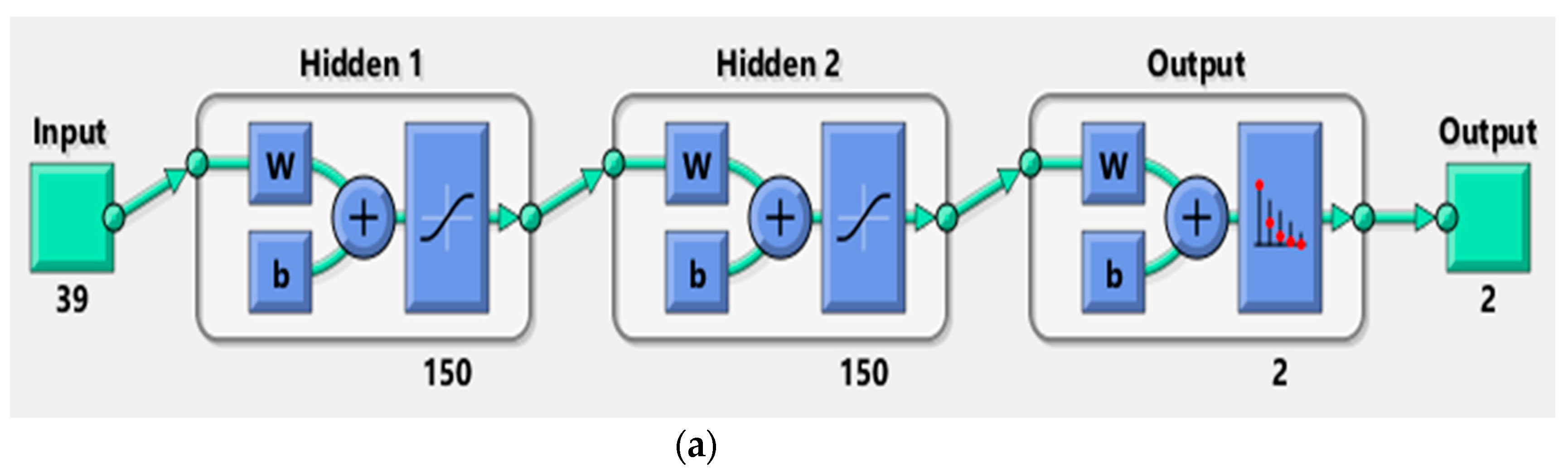
ANN is a data-processing system made up of many simple, interconnected processing components called neurons that are interconnected so that each neuron’s output functions as one or more other neurons’ input. The neurons are organized into layers in a parallel architecture inspired by the cerebral cortex of the brain, which has a superior ability to interpret and analyze complicated data and create clear and explanatory patterns to solve complicated issues [11]. There are two main kinds of layers: hidden and output layers; the data are fed into the hidden layer and then processed and delivered to the output-layer neurons, where they are compared to the required output, and the network error is calculated [38]. In our work, we utilized a backpropagation artificial neural network to classify the medical images according to the computed features for distinguishing the normal and abnormal lungs in the first medical dataset and the benign and malignant skin lesions in the second medical dataset. The neural network performance relies on the network architecture [39]. Figure 10 shows the network structure for training the first and the second medical datasets. The network input layer has 39 inputs for the first dataset and 16 inputs for the second dataset, two hidden layers, and two output layers.
To construct, train, and test the neural network for disease (skin cancer and lung disease) diagnostics, the ANN architecture mentioned above and the feed-forward backpropagation-learning algorithm were utilized. Datasets were divided into two sets, training and testing. The important parameters were determined, the learning rate was set to 1, the maximum number of epochs was set to 1000, the training time was infinity, the data-division function was used (divide rand), the transfer function of the i-th layer hyperbolic tangent sigmoid transfer function was utilized (tansig), the activation function was chosen for the output layer (softmax) which is considered a good function to assign the input image’s probability distribution to each of the classes in which the network was trained, the performance function was set to (mse) to minimize the error between actual and predicted probabilities, and the training function was a backpropagation function; weights were created randomly.
- 2.
- K Nearest Neighbor (K-NN) Classifier
K-NN is a one-of-a-kind instance-based prediction model; the testing sample’s class label was decided by the bigger part class of its k-nearest neighbors according to their Euclidean distance [40]. For the K-NN algorithm, a data sample was compared to other data samples using a distance metric [41]. There were two phases to the algorithm: the training phase and the testing phase.
Training phase: The classifier fed the patterns of features and class labels of normal and abnormal images for lung images and of benign and malignant skin lesion images using the feature characteristics that were extracted during feature extraction.
Testing phase: An unidentified test pattern was provided and, using the knowledge learned through the training phase, the unidentified pattern was classified and plotted once more in the feature space, each sample image and its properties were represented as a point in an n-dimensional space known as a feature space, and the number of features that were employed to characterize the patterns determined their dimension [42].
- 3.
- Support Vector Machine (SVM) Classifier
SVM is a popular algorithm that is widely utilized in disease diagnosis. The main idea of SVM is to utilize hyperplanes to discriminate between different groups. This classifier tries to identify the hyperplane (decision boundaries) that aids in building the effective separation of classes according to statistical-learning theory [43]. The fundamental algorithm is based on the idea of “margin,” or either side of a hyperplane that divides two classes of data. The fundamental goal of the SVM classification system is to find an overview that differentiates positive from negative data with the least amount of error [44].
- 4.
- Naïve Bayes (NB) Classifier
NB is a statistical classifier that utilizes the Bayes theorem as an underlying concept. A supervised learning-based Bayesian approach contains two phases: the learning phase and the testing phase. During the learning phase, an estimation is created based on the applied attributes, which keeps track of these attributes and categorizes their features; in the testing phase, predictions are produced based on the learning phase, and the likelihood of the desired outcome is calculated when new test data are tested. These characteristics offer a self-sufficient benefit in the development of the result [45].
- 5.
- Decision Tree (DT) Classifier
DT is a tree-structured classifier that has two nodes: decision node and leaf node. Decision nodes make decisions and have numerous branches, whereas leaf nodes display the outcomes of those decisions and do not have any additional branches. The features of the given dataset are used to perform the test or make the decision. It is called a decision tree because, like a tree, it starts with the root node and then extends to form more branches and a tree-like structure [46]. The most extensive DT algorithm for classification is C4.5. The C4.5 algorithm was employed in this work to classify lung images and melanoma skin cancer images.
- 6.
- Random Forest (RF) Classifier
RF is a supervised machine-learning technique that utilizes several decision trees on different subsets of a given dataset and takes the average to enhance the expected accuracy of that dataset. Rather than relying on a single decision tree, RF accumulates forecasts from each tree and estimates the ultimate output according to the majority vote of the predictions [47]. Each decision tree is constructed using randomly sampled training data and splitting nodes with subsets of features. The input is provided at the top of a decision tree, and as it passes down, the data are bucketed into smaller and smaller sets. RF is generated in two stages: the first is the combining of N decision trees to generate the random forest, and the second is making predictions for each tree produced in the first stage [48].
- 7.
- Random Subspace (RS) Classifier
The RS approach is a methodology for ensemble learning. The idea is to promote variety among ensemble members by limiting classifiers to working on distinct random subsets of the complete feature space. Every classifier learns with a subset of size n drawn at random from the entire collection of size N [49]. Because it uses subspaces of the real data size, this method is extremely advantageous because smaller parts can be better trained. Researchers are interested in this method because it reduces overlearning, introduces a broad model, requires less training time, and has an easier-to-understand and more straightforward structure than other classical models [50].
- 8.
- Logistic Regression (LR) Classifier
LR is a machine-learning method utilized to process classification problems. An LR model is built on a probabilistic foundation, with projected values ranging from 0 to 1. There are three kinds of LR: binary logistic regression, multinomial logistic regression, and ordinal logistic regression, and the most popular utilized case is binary logistic regression, where the result is binary (yes or no). LR employs the cost function, sometimes known as the sigmoid function. Each real number between 0 and 1 is transformed by the sigmoid function. LR can be used in the medical field to determine whether the ROI is normal or abnormal and whether a tumor is either benign or malignant [51,52].
- 9.
- Fuzzy logic Classifier
Fuzzy logic is a mathematical approach to computing and inference that uses the concept of a fuzzy set to generalize classical logic and set theory. Fuzzy inference involves all the components outlined in membership functions, logical processes, and if–then rules. FIS (Fuzzy Inference System) is a system that maps inputs (features) to outputs (classes) using fuzzy set theory [53]. To build an FIS, first, we chose the input numerical variables, which should be precise, and determined their ranges for each term. The correspondence between the input values and each fuzzy set were then defined during the fuzzification stage; this was accomplished through the use of membership functions, which reflect the degree to which a parameter value belongs to each class. The set of fuzzy rules that characterize FIS rules using logical operators, as well as the method for merging fuzzy outputs from each rule, were then described, finally extracting the output distribution from a mixture of fuzzy rules, followed by defuzzification to obtain the crisp classification result [54].
- 10.
- CNN of DL Classifier
CNNs are the best type of deep-learning model for image analysis. CNN is made up of numerous layers that use convolution filters to convert the input. The performance of CNN relies on the network architecture [55]. CNN is made up of a series of layers that form its architecture, in addition to the input layer, which is commonly an image with width and height. There are three primary layers: (1) The convolutional layer: this layer is made up of several filters (kernels) that can be learned via training. The kernels are tiny matrices with real values that can be interpreted as weights. (2) The pooling layer: this layer is employed after a convolution layer to minimize the spatial size of the generated convolution matrices; as a result, this strategy decreases the number of parameters to be learned in the network, which contributes to overfitting control. (3) The fully connected layer: this layer connects each element of the convolution output matrices to an input neuron. The output of the convolutional and pooling layers represents the features extracted from the input image [56,57].
In this work, we suggested and assessed a deep convolutional neural network structure for diagnosing lung diseases and melanoma skin cancer. We performed an ablation analysis of the proposed structure and tested other topologies to compare their results with the results of the proposed CNN structure. We also manually tested extracted features in this work on the proposed CNN structure and compared the results.
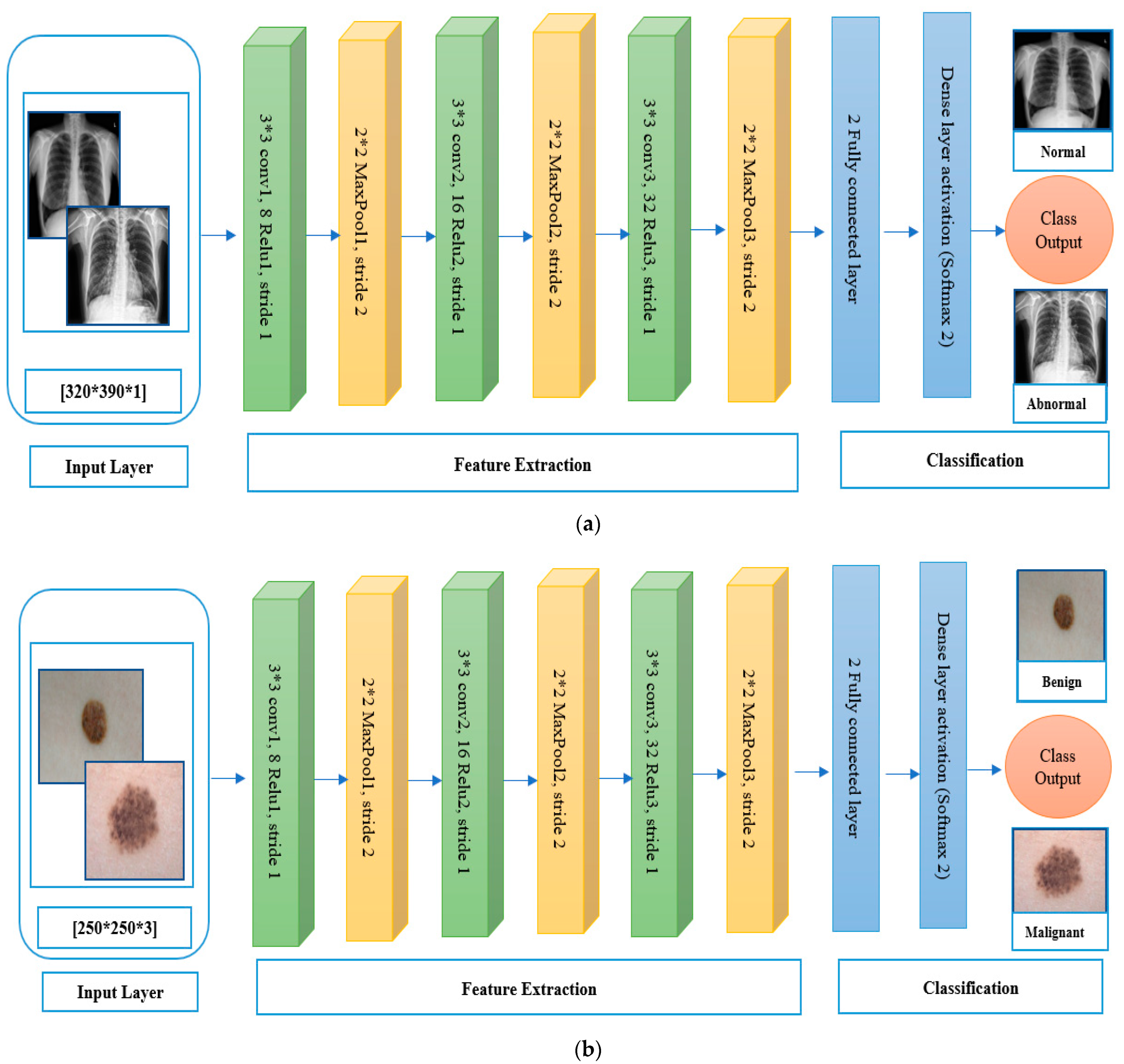
The proposed CNN architecture used to resolve our classification problem is shown in Figure 11. The model contains three convolution layers, three max-pooling layers, three batch-normalization layers, and a fully connected layer. When the image was input into the CNN structure, the image was represented as image height × image width. The image size was standardized in the system to obtain robust outcomes. After the image passed through the convolutional layers, the feature map included the feature depth, represented as image height × image width × image depth. Filter size, stride, and padding zero were the most important parameters of the convolutional layers that impacted the performance of the convolutional layers. Convolutional layers wrapped with the filter size (in this case, we used a 3 × 3 matrix to achieve more precision when traversing the matrix containing the images) around the image, learned the weights through the training phase, processed the input, and passed it to the next layer. Zero padding was the process of filling neurons with zeros to maintain the size of the resulting neurons. When zero padding was one, the neurons were padded with a row and a column around the edges. Rectified linear unit (ReLU) layers were also utilized after convolutional layers for image processing. The objective of ReLU was to pass the positive output and repress the negative output. The dimensions were decreased by the pooling layer, as the dimensions of the image were decreased by grouping numerous neurons and representing them in one neuron based on the maximum or average method, which is named the max-pooling layer. The maximum value of the groups of neurons was chosen utilizing the maximum method, and the average value of the neurons was selected utilizing the average method. In the fully connected layers, the last layer of the convolutional neural networks, each neuron was connected to all neurons. Feature maps were transformed into flat representations (unidirectional). Softmax is the activation function utilized in the last phase of the convolutional neural network model; it is nonlinear and is utilized in multiple classes.
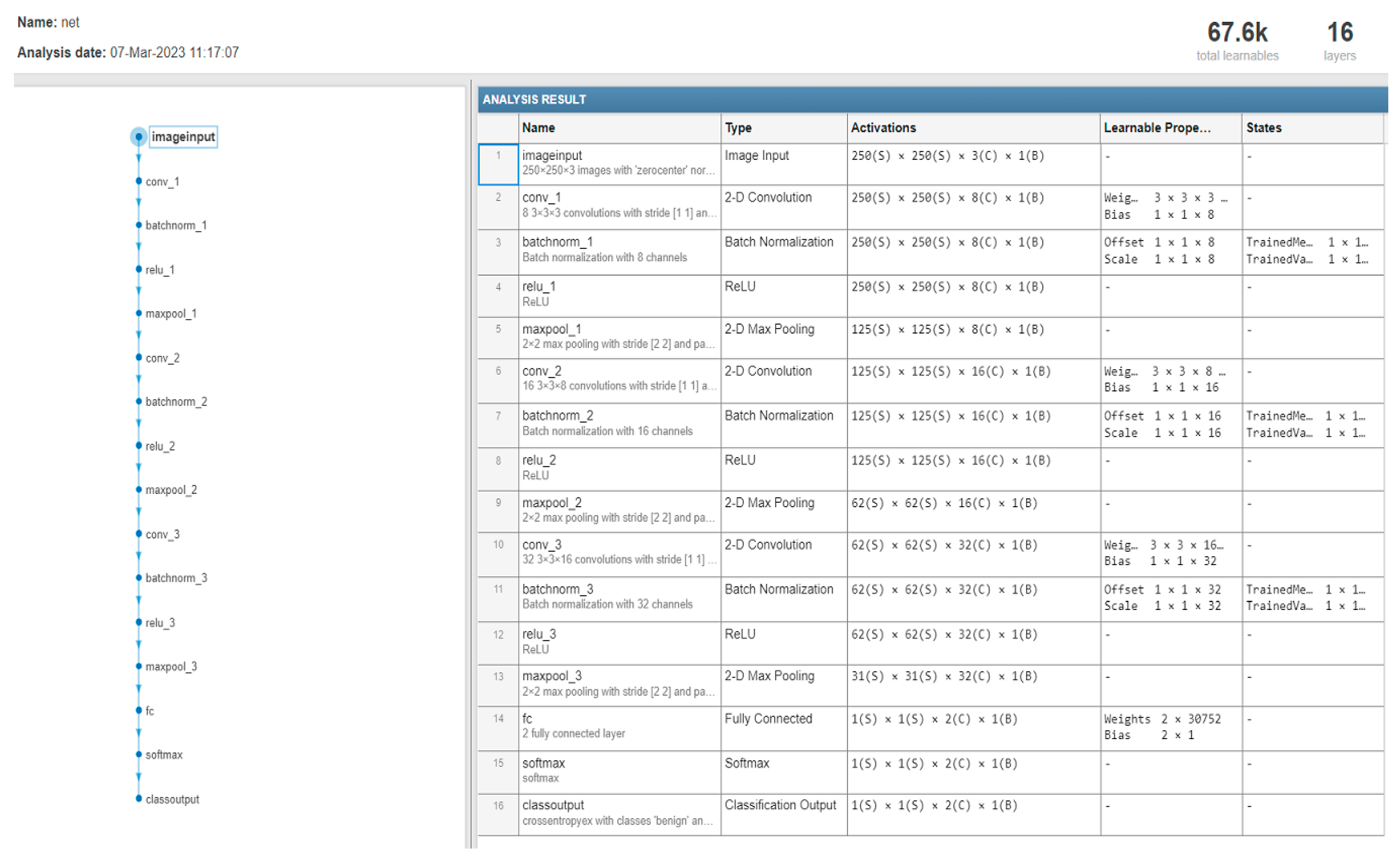
Figure 12 describes the number of layers, the size of each filter, and the parameter of the CNN structure that was used in diagnosing the two medical datasets (chest X-ray and melanoma skin cancer).
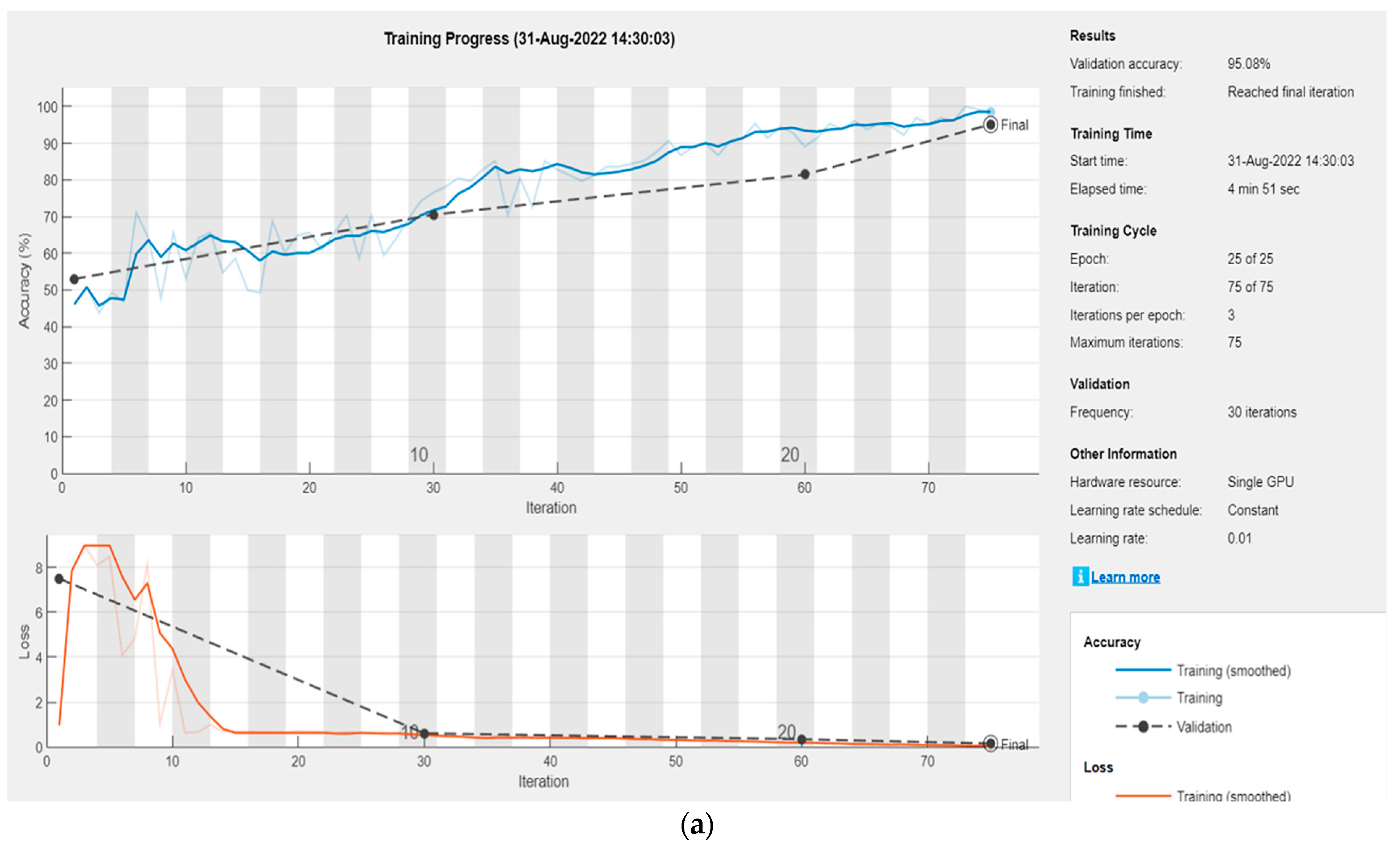
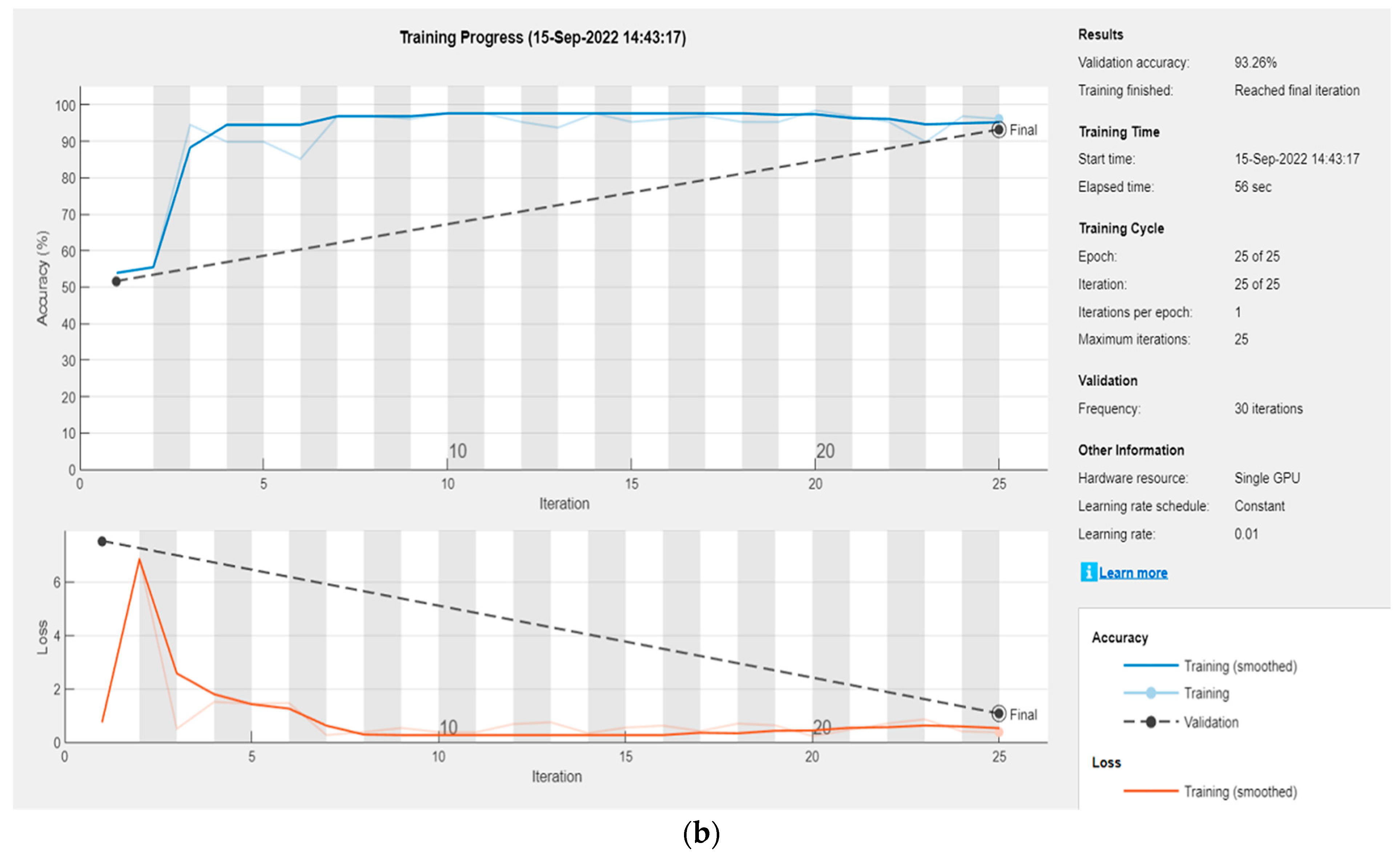
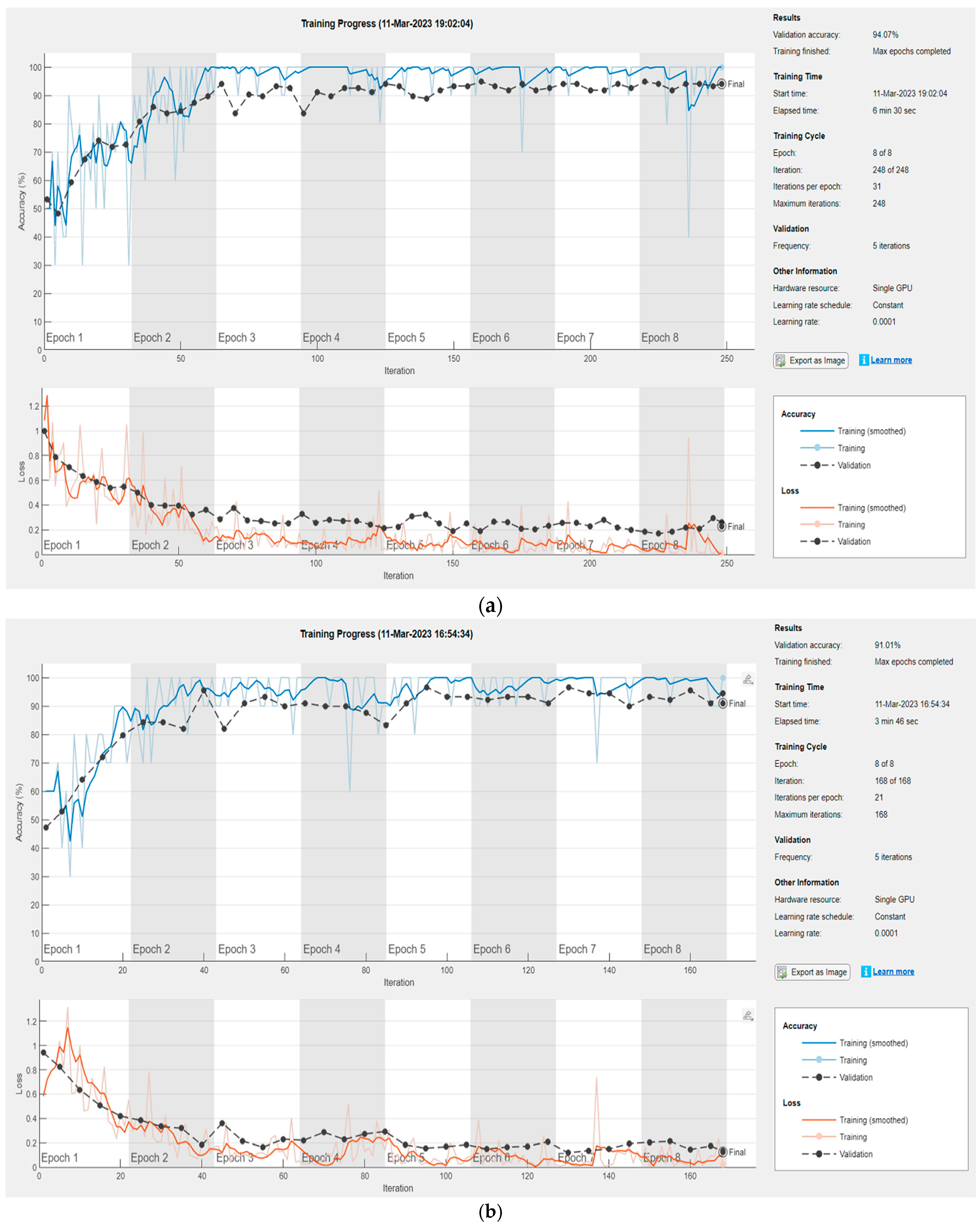
Figure 13 illustrates the results of the datasets (lung X-ray and melanoma skin cancer dermoscopy) classification by the proposed CNN structure.
As can be seen from the confusion matrices for the first and second medical image datasets in Figure 14, for the lung dataset, we used 612 samples that were classified as 288 normal and 324 abnormal. The samples were divided by CNN into 70% for training and 30% for testing. The number of samples for training was 429 (227 samples for abnormal and 202 for normal). The number of samples for testing was 183 (97 for abnormal and 86 for normal), and for the skin cancer dataset, we used 300 samples that have been classified (145 benign and 155 malignant). The samples were divided by CNN into 70% for training and 30% for testing. The number of samples for training was 211 (102 samples for benign and 109 for malignant). The number of samples for testing was 89 (43 for benign and 46 for malignant); the accuracy of the classification for the first medical dataset was 95% in the last epoch at 25 epochs, 75 iterations, and the learning rate was equal to 0.01; the accuracy of the classification for the second medical dataset is 93% in the last epoch at 25 epochs, 25 iterations, with a learning rate equal to 0.01.
Ablation analyses of the proposed CNN: Some ablation tests were conducted through the three crucial parameters: the number of layers, the kernel size, and the network parameter. The number of layers is the first critical network parameter, and it is directly proportional to the network’s description capabilities. Nevertheless, having more layers means having more variables to optimize, which necessitates even more training data, without which overfitting occurs. Given the restricted amount of samples available and the insignificant impact of additional layers (up to 25 were evaluated), we determined that three convolution layers, three max-pooling layers, three batch-normalization layers, and a fully linked layer were sufficient for our architecture to obtain good results, but when trying to remove any layer from the suggested architecture, the result started to deteriorate. Table 7 shows the results of the ablation test for the first parameter (the number of layers) for the two medical datasets.
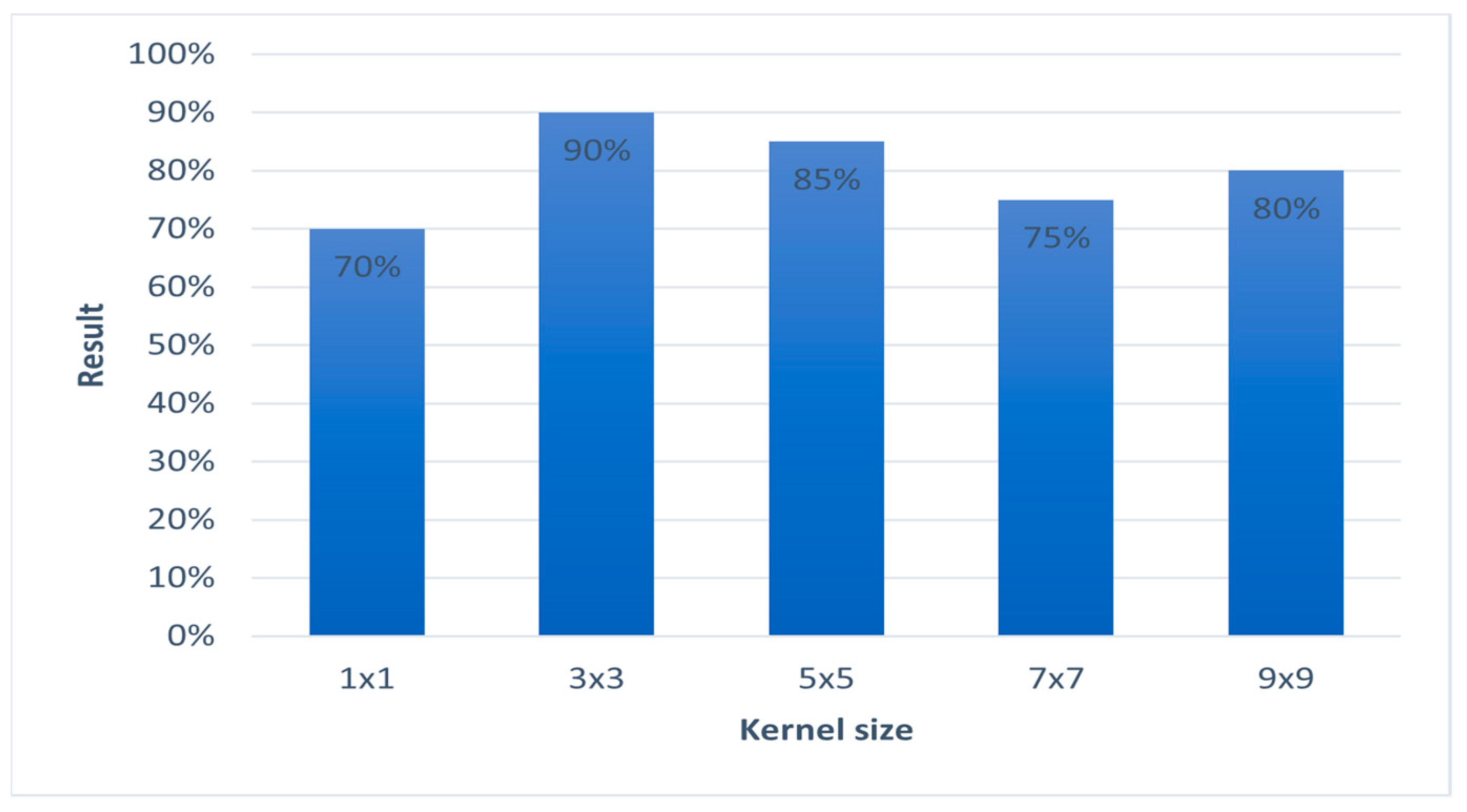
As far as the kernel size is concerned, experiments were conducted from 1 × 1 up to 9 × 9 pixels. The 3 × 3 size in each convolutional layer had a strong positive impact, which, nevertheless, did not increase with a larger spatial radius; regardless, with the size of 3 × 3, we achieved an accuracy of more than 90% for the two sets of selected medical databases. Figure 15 shows the relative results of ablation test for the second parameter (kernel size) for the two medical datasets.
As far as the crucial network parameters, we conducted experiments on the most important network information:
- Learning rate (LR): The network’s learning rate is inversely proportional to convergence speed. We experimented with a large spectrum of values; however, their effect on overall performance was insignificant and the model did not exhibit pathological behavior. The training of the proposed CNN network was realized with a learning rate of 1 × 10⁻².
- Epochs: We selected 25 epochs for training the network because training over many epochs is common in applications and often results in greater potential for overfitting, 25 epochs were enough to train the datasets and obtain good accuracy.
- Activation function: We conducted several experiments on choosing the activation functions and changing the function in each experiment (we used several activation functions commonly used like the sigmoid function, and the hyperbolic tangent tanh(x)), but we did not obtain satisfactory results for the proposed network except in the case of activation functions for the ReLU and softmax, because it is considered the most effective activation function. In comparison to sigmoid and tanh, ReLU is more trustworthy and speeds up convergence by six times.
Through experiments with regard to these main parameters in the network, it is not possible to remove any one of them because removing them from the network architecture may lead to a deterioration in the result, or it may not work.
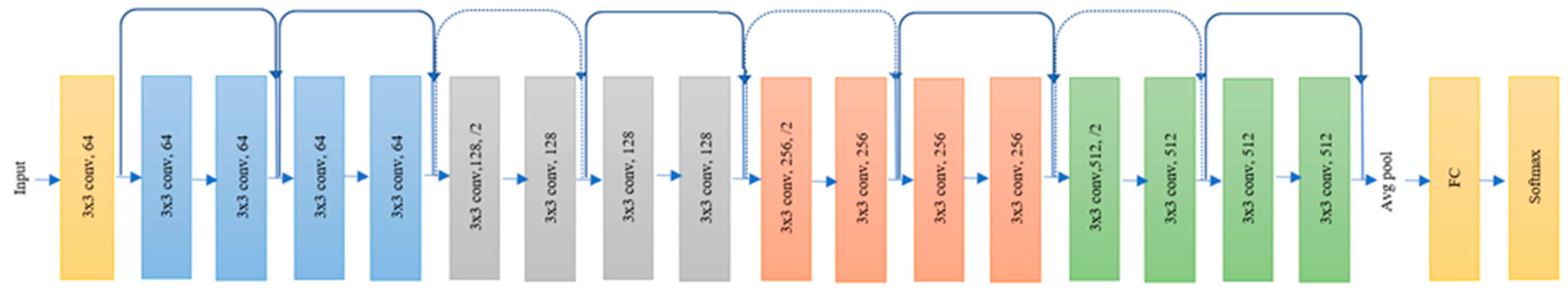
- Test different topologies: Some advanced CNNs have more complicated topologies and network architecture for different tasks, for example, GoogLeNet, ResNet, AlexNet, VGGNet, and inception modules. In this work, we tested the ResNet18 model to compare the result with the proposed CNN structure result. The ResNet model’s architecture is shown in Figure 16.
Figure 16.
Representing original ResNet-18 architecture [58].
Figure 16.
Representing original ResNet-18 architecture [58].

ResNet18 has 18 layers, the first of which is a 7 × 7 kernel. It has four identical layers of ConvNets. Each layer is made up of two residual blocks. Each block is made up of two weight layers connected by a skip connection to the output of the second weight layer through a ReLU. If the result equals the ConvNet layer’s input, the identity connection is used. If the input and output are not similar, convolutional pooling is performed on the skip connection. The ResNet18 input size is (224, 224, 3), which is achieved through preprocessing augmentation with the AugStatic package. In (224, 224, 3), 224 denotes the width and height. The RBG channel is number three. The result is an FC layer that feeds data to the sequential layer [59,60]. We tested the two selected medical databases in this work on the ResNet18 model and changed the size to 224 × 224 × 3 to fit with the network input to compare the result of the network ResNet18 with the proposed CNN network. The table shows the comparison results for the two medical datasets.
Figure 17 describes the detailed structure of the part of the ResNet18 model (the number of layers, the size of each filter, and the parameter of the ResNet18 model).
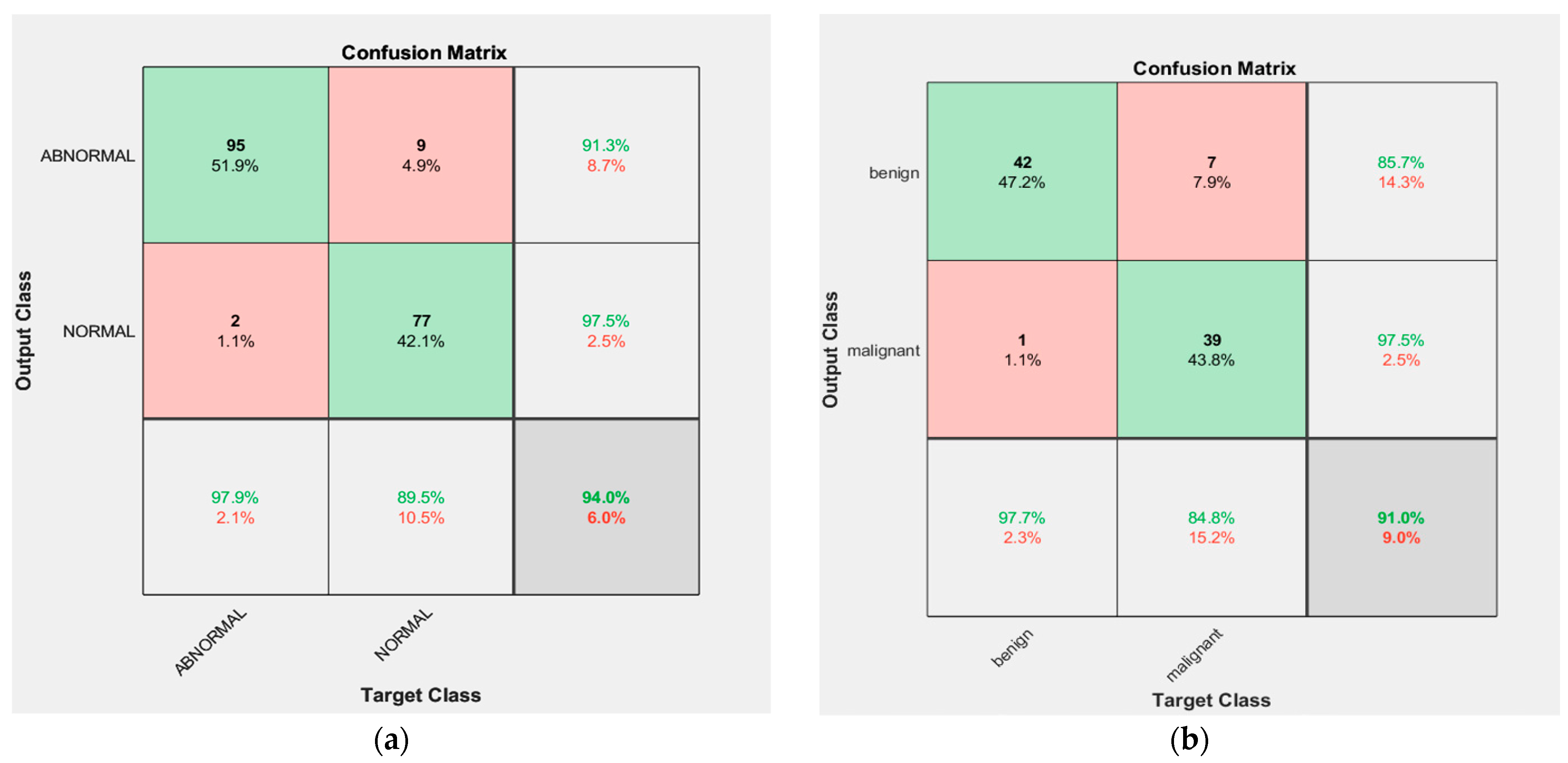
Figure 18 illustrates the results of the dataset (lung X-ray and melanoma skin cancer dermoscopy) classification by the ResNet18 model.
As can be seen from the confusion matrices for the first and second medical image datasets in Figure 19, the accuracy of the classification for the first medical dataset is 94%, and 91% for the second medical dataset.
From Table 8, it can be seen that the proposed CNN structure outperformed ResNet18. It has been noticed that as the number of added layers increases, training neural networks becomes more difficult, and in some cases, accuracy reduces. Through experiments, we found that the proposed CNN structure is sufficient to classify the selected medical databases and obtain good results. In addition, the proposed network takes less time to train, and this is one of the important advantages that made us adopt the proposed structure in the diagnosis of the selected medical databases.
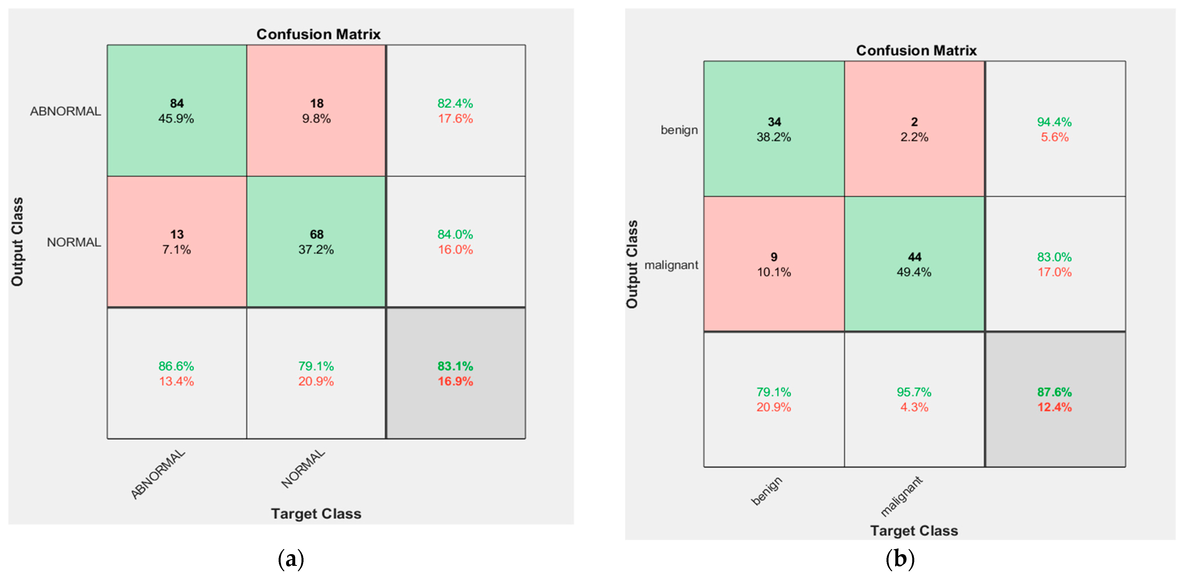
Additionally, we tested the performance of the proposed CNN structure in the case of the inputs of extracted features for the other ML methods concatenated to the final layer. As can be seen from the confusion matrices for the first and second medical image datasets in Figure 20, the accuracy of the classification for the first medical dataset is 83.1%, and 87.6% for the second medical dataset, in the case of training the network using the extracted features manually. Therefore, the performance of the network using the features extracted manually is less efficient; we noticed through experiments that the features extracted from the network are more robust and effective, and suit the performance of the network and provide better results. Therefore, the proposed CNN network structure was adopted in the diagnosis of the selected medical dataset in this work because it achieved high accuracy in diagnosis.
Table 9 shows a comparison of the classification methods used in this work in terms of the most important advantages and disadvantages of each one.
4.3.2. Model Evaluation and Validation
This stage is the primary metric for assessing the performance of the classification models. Lung diseases and melanoma skin cancer can be classified as true positive (TP) or true negative (TN) if correctly diagnosed, or false positive (FP) or false negative (FN) if incorrectly diagnosed. Accuracy, sensitivity, specificity, precision, recall, F-measure, and AUC (area under curve) are the most popular assessment metrics used for lung diseases and melanoma skin cancer classification. We describe these metrics briefly below [11,41]:
Accuracy (Acc): This metric measures the number of correctly classified cases; it can be represented utilizing the following equation:
Sensitivity (Sn): This metric reveals the number of correctly estimated total positive cases; it can be represented utilizing the following equation:
Specificity (Sp): This metric reveals the number of correctly estimated total negative cases; it can be represented by the equation:
Precision (Pr): This metric indicates how accurate the overall positive forecasts are; it can be represented by the equation:
Recall: This metric reveals how well the total number of positive instances is predicted; it can be represented by the equation:
F-Measure: This metric is a way of checking how accurately the model operates by distinguishing the right true positives from the expected ones; the following equation can be used to express it:
AUC: This metric is one of the most important evaluation metrics for measuring the performance of any classification model and is used to summarize the ROC curve, which represents the area under the ROC curve. The greater the AUC, the better the model distinguishes between positive and negative classifications, and it can be represented by the equation [58]:
5. Results and Comparison
This section introduces the outcomes of all the methods utilized in the classification, which were implemented using Matlab 2021, as well as a comparison of the results.
The results of the feature extraction for some samples of the first medical dataset (chest X-ray dataset) and the second medical dataset (melanoma skin cancer dermoscopy dataset) for the feature extraction methods used in this work are introduced in Appendix A.
The results of various classification algorithms are described in Table 10 and Table 11, where the performance metrics for all ML algorithms and deep-learning CNN that were applied to the chest X-ray dataset and melanoma skin cancer dermoscopy dataset are described.
From Table 10, it can be noted that classification based on a random forest (RF) algorithm performs better than other machine-learning techniques applied to lung datasets in terms of performance metrics, and CNN for deep-learning classification provides better outcomes than all other algorithms when applied to X-ray lung diseases. LR, ANN, KNN, SVM, and RS are also effective algorithms for classification issues, and they perform well in the issue at hand.
From Table 11, it can be seen that classification based on the ANN algorithm outperforms all the other ML algorithms that were applied to melanoma skin cancer datasets in terms of performance metrics. Other algorithms such as KNN, RF, RS, Fuzzy Logic, and CNN are also effective algorithms for classification issues, and they perform well in the issue at hand.
Table 12 shows the comparison of the test accuracy of the classification algorithms applied to the two medical image datasets used in our work.
From Table 12, we notice that CNN and ANN were the highest-performing classifiers for the lung disease and skin cancer disease classification, respectively. This is due to the characteristics of the CNN network (the number of layers and the number of filters that were utilized in addition to the efficiency of the activation functions) and the superior ability of DL networks in classification tasks, especially CNNs, which are considered to be the state-of-the-art systems for image classification, especially in the classification of medical databases.
For an ANN network, the classification accuracy was high if the extracted features were strong and good for classification, the network structure was good, and the number of layers was large (we used many layers and 150 complex neurons for each hidden layer), in addition to the efficiency of the activation functions utilized in the network (the activation function was chosen for the output layer (softmax) which is considered a good function to assign the input images’ probability distribution to each of the classes in which the network was trained).
To check the accuracy of the final optimized model, a new set of 100 images from the medical datasets used in this work was used for validation. Table 13 shows the results of the validation accuracy of the classification algorithms applied to the two medical image datasets used in our work. We note that the results of the validation are very close to the test results of the classification algorithms applied to the two medical image datasets, shown in Table 12.
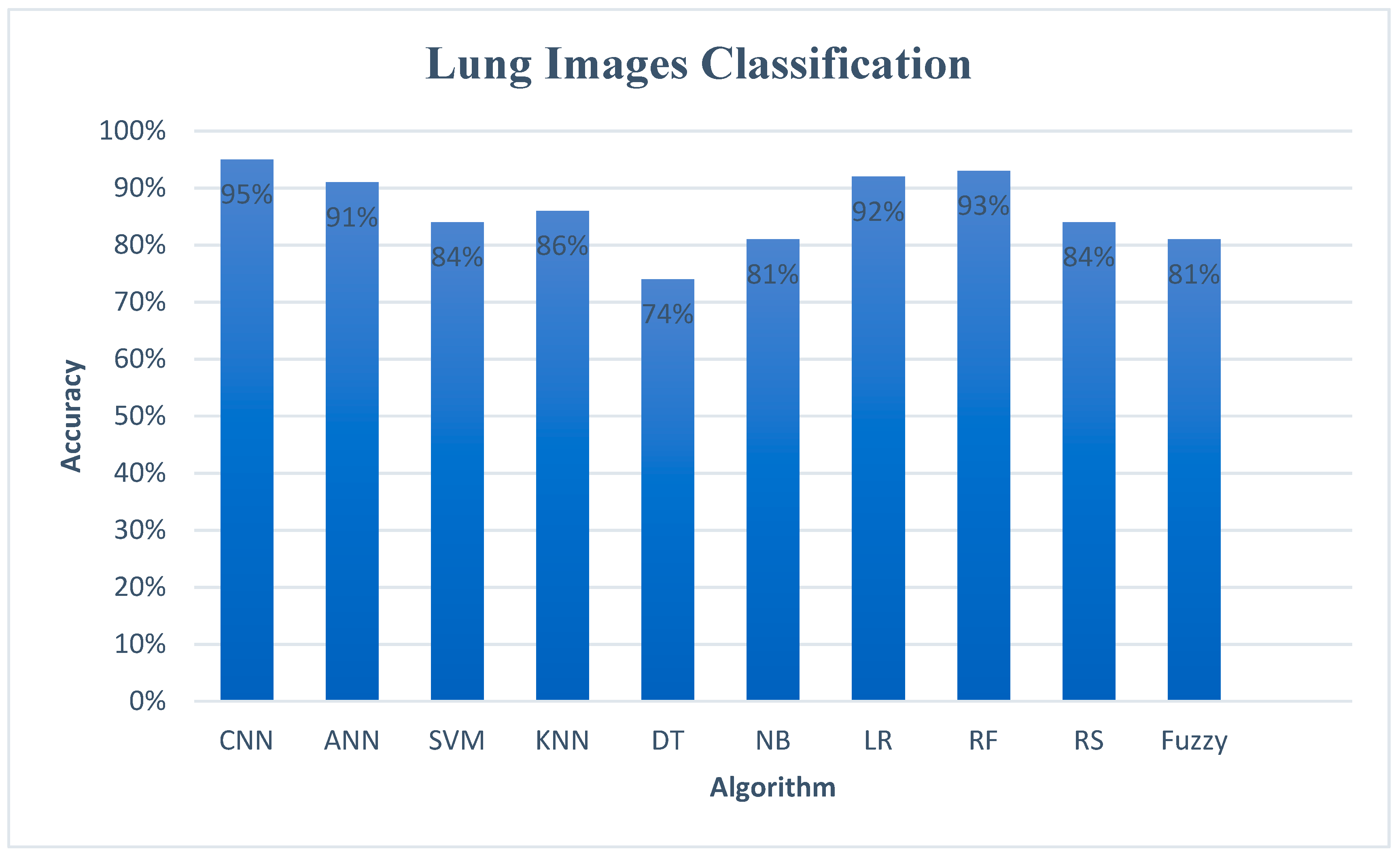
Figure 21 shows the comparison of the accuracy of the classification algorithms for the lung dataset.
Figure 22 shows the comparison of the accuracy of the classification algorithms for the melanoma skin cancer dataset.
As seen in Figure 21, the highest accuracy was 95% for the CNN algorithm. For the machine-learning algorithms, the highest accuracy was 93% for the RF algorithm, followed by the LR and ANN algorithms with an accuracy of 92% and 91%, respectively. On the other hand, the DT classifier attained the lowest performance of 74%.
As seen in Figure 22, the highest accuracy was 96% for ANN, followed by the KNN, RF, and RS algorithms, with an accuracy of 95%, 94%, and 93%, respectively, for ML algorithms. Additionally, the CNN algorithm attained a high accuracy of 93%. On the other hand, the NB classifier attained the lowest performance of 80%.
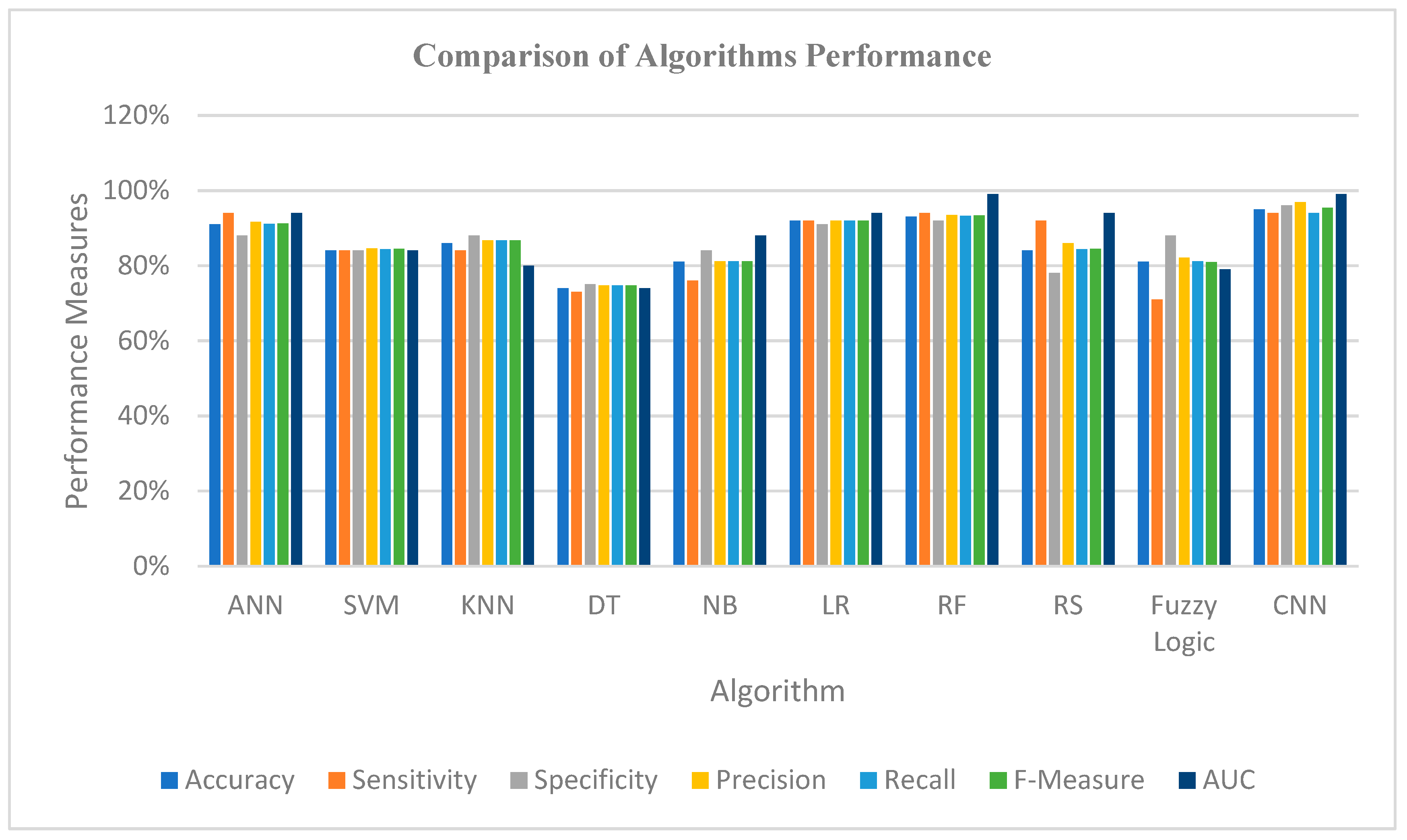
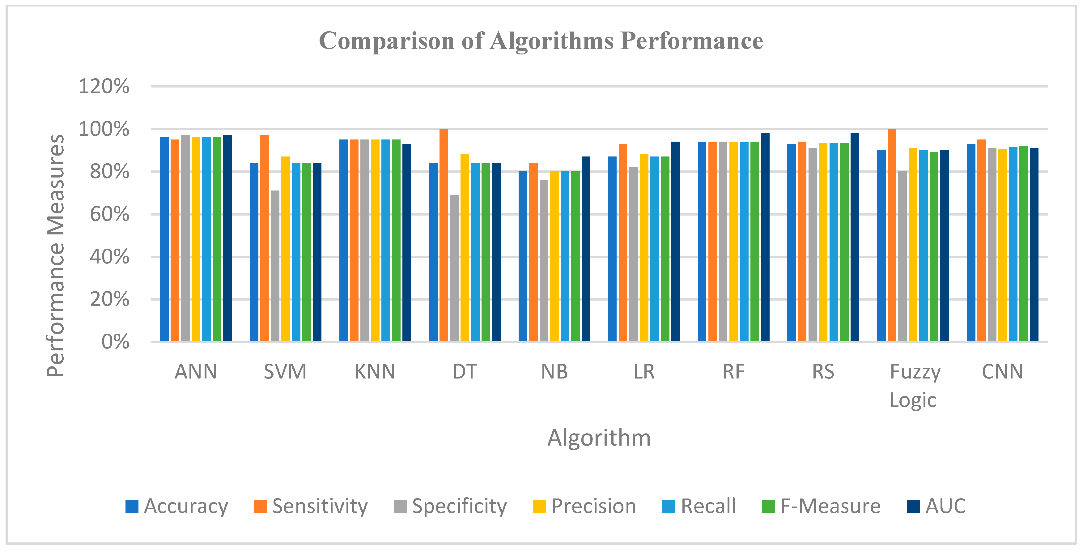
Figure 23 and Figure 24 show the graphical representation of the performance measures for the algorithms applied to the lung dataset and the melanoma skin cancer dataset, which shows a comparison of the performance measures in terms of accuracy, sensitivity, specificity, precision, recall, F-measure, and AUC.
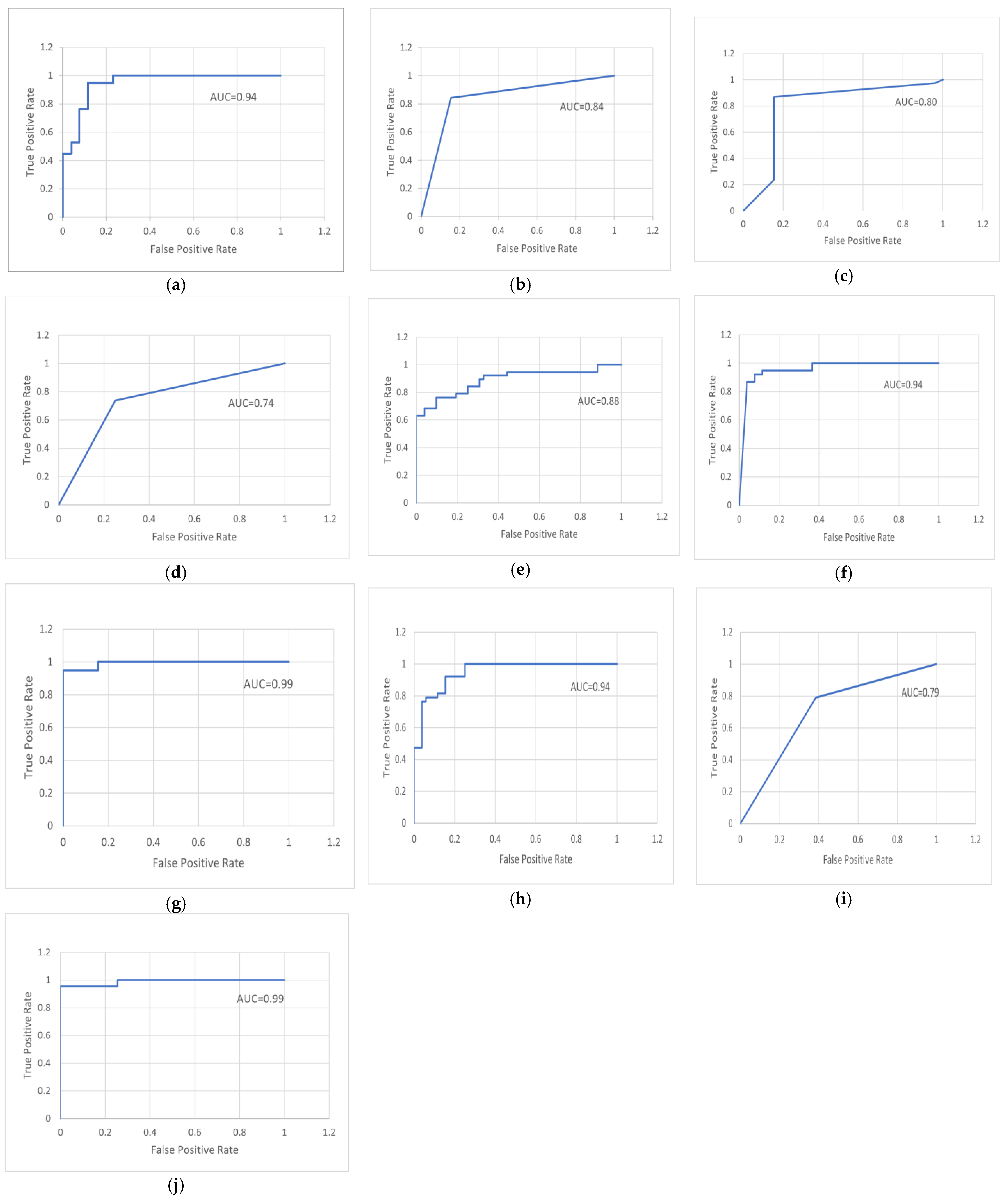
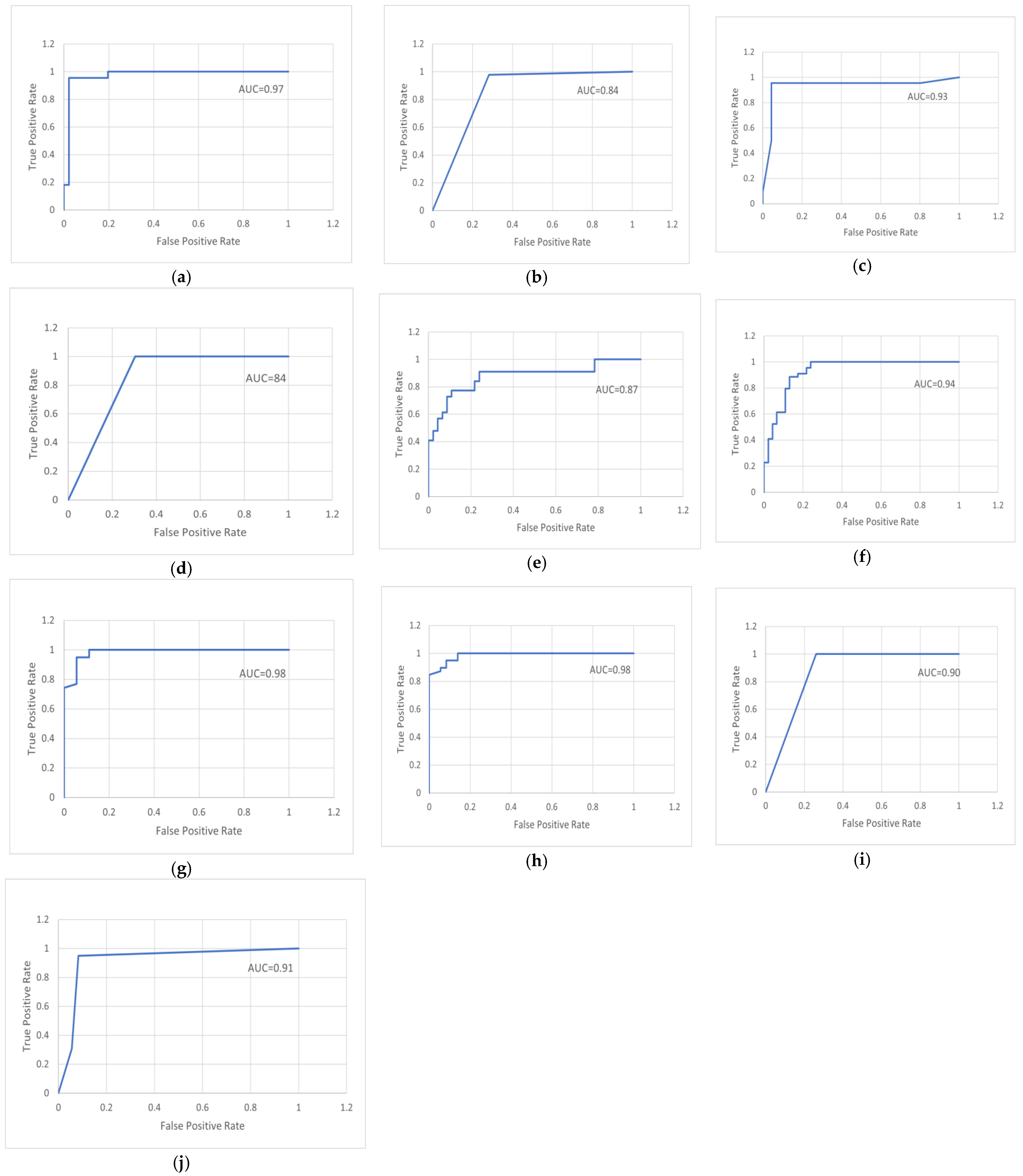
Figure 25 and Figure 26 illustrate the receiver operating characteristic (ROC), which is a system performance curve used in medical testing for diagnosing medical datasets. A ROC curve is constructed by plotting the true-positive rate (TPR) against the false-positive rate (FPR). The true-positive rate is the fraction of all positive observations that were correctly expected to be positive. The false-positive rate is the proportion of negative observations that were wrongly anticipated to be positive. Each figure represents an assessment curve for ten methods for each database.
6. Contributions
The essential contributions of this work are summarized as follows:
- We exploited ML and DL to find the most precise techniques for diagnosis to provide directions for future research.
- We analyzed more than one medical image database to evaluate more than one disease using the proposed system.
- By improving the raw images, finding the ROI (lung and lesion), extracting ROI-specific features, and applying ML and DL algorithms for automatic classification, we present an integrated framework for identifying lung disease utilizing chest X-ray scans and melanoma skin cancer using skin dermoscopy.
- We suggest an algorithm for image preprocessing, where the raw X-ray images were processed and their quality was improved. Additionally, an algorithm was proposed to remove hair from dermoscopy skin images to enhance them and obtain a precise diagnosis. The proposed preprocessing algorithms provided good results in the work.
- We suggest an algorithm for image segmentation to separate the ROI from the image to extract only lung regions from chest X-ray images and lesion regions from dermoscopy skin images. The proposed segmentation algorithms achieved good results in the work.
- We extracted a robust collection of features from ROI (lung and skin lesion) images, including color, texture, shape, and geometry features to help us achieve satisfactory results in the classification.
- Good results were obtained for the proposed system, utilizing two scalable datasets and an appropriate training-to-testing ratio of 70% to 30%. The CNN model and machine-learning techniques such as SVM, KNN, ANN, NB, LR, RF, RS, and fuzzy logic were trained for assessment. In the end, the results of the suggested model methods were compared.
7. Concluded Discussion and Future Directions
In this section, we discuss the techniques utilized in this work, and the medical dataset utilized to diagnose diseases through discussion and future directions.
7.1. Discussion
In this work, chest X-ray and melanoma skin cancer dermoscopy datasets were used for classification purposes. The data were divided into 70% for training and 30% for testing. The data were analyzed by applying the main analysis processes, where the medical data images were preprocessed to remove noise and improve contrast. Some filters were applied to improve the images; the chest X-ray images were preprocessed using the median filter and applying the contrast adjustment with the histogram equalization enhancement to improve the images and remove noise. Hair was removed from the melanoma skin cancer images using the algorithm proposed in the work to improve the images and prepare them well for the next stage of the analysis, which was to separate the object of interest from the rest of the image.
The suggested segmentation algorithms were applied to separate the lung the from chest X-ray images by using thresholding and morphological operations, and to separate the lesion from skin cancer images using Otsu thresholding with binarization and negation processes. The proposed segmentation algorithms provided excellent results in separating the object from the image to move to the other stage, which is the extraction of features. Here, the best methods were applied to obtain the most relevant features from the images such as texture and shape, extracting features from lung images and lesion images, such as color, texture, and some geometry features, and to move to the most important stage, which is the classification.
At this point, we applied a set of the most important and best common classification methods based on machine learning such as ANN, SVM, KNN, DT, NB, LR, RF, RS, and fuzzy logic in addition to CNN for deep learning to identify the performance of these algorithms and the accuracy of their classification. All these were realized by training the selected databases and obtaining results, where most of the methods proved effective in diagnosing lung diseases and melanoma skin cancer and showed good results.
The model was evaluated using accuracy, sensitivity, specificity, precision, recall, and F-measure. However, the analysis of the results indicates that there is enough space to improve the performance obtained for some methods by applying other techniques that may be hybrid or improved methods to increase the speed of performance and reduce the time, cost, and effort in diagnosing diseases. The comparison in the application of diagnostic and evaluation methods to both sets of medical image datasets revealed that the accuracy and performance of the algorithm depend on the type of the medical dataset, the amount of data, the type of disease, and the performance of the methods applied in the preprocessing, segmentation, and feature-extraction stages.
In particular, the results of the applied classification methods are generalizable to the diagnosis of the selected databases, even if this work focused on classifying melanoma skin cancer and lung diseases.
In general, the results of the classification algorithms utilized in this work can be generalized to all medical data if appropriate preprocessing methods are applied to treat databases because each database differs in its processing according to the conditions of taking pictures and the noise in the images. However, through what we have seen in this work, the step of extracting the most relevant features from the images differs depending on the type of dataset. For this reason, we conducted our experiments and tested two different specific types of medical databases to diagnose two different diseases and, in this way, create a model that shows its capacity for generalization.
7.2. Future Directions
In future work, we suggest the following:
- Increase the number of diseases that are diagnosed and employ other classifiers.
- We also plan to work with more sophisticated medical image data.
- Employ new sets of features for more medical images, to improve performance.
- Although good findings were produced in this work, more research should be conducted by merging the algorithms employed in classification or by adding optimization tools.
- There is a need to develop or create a new classification system for the diagnosis of diseases based on medical image databases.
- Further extensive studies or experiments with vast datasets and hybrid or optimized classification approaches are necessary.
In the future, we plan to work on a new classification model architecture by building a hybrid classifier by merging two or more of the classification methods that we used in this work or by improving one of the classifiers used by adding tools for improvement to increase the speed of performance and reduce the time, cost, and effort in diagnosing diseases, and applying the new system to more than one database that includes types of diseases, to prove its effectiveness and increase the percentage of generalizing the system on the most diseases that pose a threat to human life and detect them early so that we can treat them.
8. Conclusions
This work examines the effectiveness of several machine-learning- and deep-learning-based classification algorithms for medical data diagnosis, and describes a machine-learning- and deep-learning-based diagnosis system for two of the world’s most serious diseases. Experiments were performed on two different medical datasets (chest X-ray dataset and dermoscopy melanoma skin cancer dataset). The following conclusions can be drawn based on the experimental results:
- Most of the classification algorithms based on machine learning that were applied to the two selected databases provided good results in terms of various classification performance metrics such as accuracy, sensitivity, specificity, precision, recall, F-measure, and AUC.
- The deep-learning-based convolutional neural network algorithm outperformed in others when applied to the two selected medical databases, as it provided high classification accuracy, reaching 95% in classifying the lung dataset into normal and abnormal, and 93% in classifying the melanoma skin cancer dataset into benign and malignant.
- Additionally, the outcomes varied from one dataset to another, according to the type of medical dataset, the type of medical imaging, and the efficiency of the methods applied in the preprocessing, segmentation, and feature extraction to classify the medical dataset; whenever the methods that were applied to a dataset to train the model were accurate and worked well, the performance of the classification model was better.
- The work provides some crucial insights into modern ML/DL methodologies in the medical field that are applied in disease research nowadays.
- Better outcomes are anticipated with the usage of hybrid algorithms and combined ML and DL techniques. Even minor adjustments can sometimes yield good results. We found that training data quality is an important consideration when creating ML- and DL-based systems.
As an outline of what we have achieved in this work, we analyzed two medical datasets (chest X-ray and melanoma skin cancer dermoscopy) by applying the main analysis processes, where preprocessing of the medical data images was conducted to remove noise and improve contrast. Hair was removed from the melanoma skin cancer images using the algorithm proposed in the work to improve the images. The suggested segmentation algorithms were applied to separate the lung from the chest X-ray images by using thresholding and morphological operations, and to separate the lesion from skin cancer images using Otsu thresholding with binarization and negation processes. Relevant features were extracted from the images for use in the classification such as color, texture, shape, and geometry features. In the classification stage, we applied a set of the most important and best common classification methods based on machine learning such as ANN, SVM, KNN, DT, NB, LR, RF, RS, and fuzzy logic in addition to CNN for deep learning to investigate the performance of these algorithms and the accuracy of their classification. The model was evaluated utilizing accuracy, sensitivity, specificity, precision, recall, F-measure, and AUC. Most of the methods proved effective in diagnosing lung diseases and melanoma skin cancer and provided good results.
Author Contributions
The concept of the article was proposed by N.P., the data resources and validation were contributed by B.M.R., and the formal analysis, investigation, and draft preparation were performed by B.M.R. The supervision and review of the study were headed by N.P. The final writing was critically revised by N.P. and finally approved by the authors. All authors have read and agreed to the published version of the manuscript.
Funding
This research received no external funding.
Institutional Review Board Statement
Not applicable.
Informed Consent Statement
Not applicable.
Data Availability Statement
The study does not report any data.
Conflicts of Interest
The authors declare no conflict of interest.
Abbreviations
ML—Machine Learning; DL—Deep Learning; ANN—Artificial Neural Network; SVM—Support Vector Machine; KNN—K nearest Neighbor; DT—Decision Tree; RF—Random Forest; NB—Naïve Bayes; RS—Random Subspace; LR—Logistic Regression; CNN—Convolutional Neural Network; ROI—Region Of Interest; RGB—Red–Green–Blue; HSV—Hue–Saturation–Value; 2-D—Two-Dimensional; RNN—Recurrent Neural Network; GLCM—Gray-Level Co-Occurrence Matrix; GLRLM—Gray-Level Run-Length Matrix; SRE—Short-Run Emphasis; LRE—Long-Run Emphasis; RP—Run Percentage; LGRE—Low Gray-level Run Emphasis; MI—Moment Invariant; CM—Color Moment; A—Area; Pr—Perimeter; Ecc—Eccentricity; D—Diameter; FIS—Fuzzy Inference System; TP—True Positive; TN—True Negative; FP—False Positive; FN—False Negative; Acc—Accuracy; Sn—Sensitivity; Sp—Specificity; Pr—Precision; AUC—Area Under Curve.
Appendix A
This section introduces the results of the feature extraction for some samples of the first medical dataset (chest X-ray dataset) and the second medical dataset (melanoma skin cancer dermoscopy dataset) for the feature-extraction methods used in this work.
Table A1 and Table A2 show the results of different random samples of the normal and abnormal lungs for the first medical dataset (chest X-ray dataset) using the GLCM texture-features method.

Table A1.
Results of normal sample lungs using GLCM features.
| Samples | GLCM Features | |||||||||||||||
|---|---|---|---|---|---|---|---|---|---|---|---|---|---|---|---|---|
| Contrast | Correlation | Energy | Homogeneity | |||||||||||||
| 0° | 45° | 90° | 135° | 0° | 45° | 90° | 135° | 0° | 45° | 90° | 135° | 0° | 45° | 90° | 135° | |
| Image 1 | 0.23 | 0.31 | 0.15 | 0.28 | 0.931 | 0.933 | 0.96 | 0.951 | 0.294 | 0.241 | 0.25 | 0.23 | 0.68 | 0.65 | 0.69 | 0.61 |
| Image 22 | 0.18 | 0.34 | 0.23 | 0.18 | 0.933 | 0.924 | 0.94 | 0.942 | 0.259 | 0.243 | 0.24 | 0.24 | 0.69 | 0.66 | 0.67 | 0.62 |
| Image 69 | 0.25 | 0.23 | 0.17 | 0.27 | 0.94 | 0.931 | 0.95 | 0.953 | 0.281 | 0.252 | 0.23 | 0.22 | 0.66 | 0.64 | 0.63 | 0.65 |
| Image 80 | 0.26 | 0.33 | 0.21 | 0.19 | 0.921 | 0.913 | 0.961 | 0.939 | 0.278 | 0.251 | 0.25 | 0.24 | 0.62 | 0.63 | 0.68 | 0.64 |
| Image 187 | 0.14 | 0.208 | 0.15 | 0.24 | 0.924 | 0.915 | 0.952 | 0.941 | 0.284 | 0.247 | 0.24 | 0.23 | 0.67 | 0.62 | 0.69 | 0.66 |
Table A2.
Results of abnormal sample lungs using GLCM features.
| Samples | GLCM Features | |||||||||||||||
|---|---|---|---|---|---|---|---|---|---|---|---|---|---|---|---|---|
| Contrast | Correlation | Energy | Homogeneity | |||||||||||||
| 0° | 45° | 90° | 135° | 0° | 45° | 90° | 135° | 0° | 45° | 90° | 135° | 0° | 45° | 90° | 135° | |
| Image 1 | 0.504 | 0.61 | 0.37 | 0.54 | 0.809 | 0.87 | 0.82 | 0.86 | 0.196 | 0.168 | 0.15 | 0.14 | 0.77 | 0.701 | 0.75 | 0.701 |
| Image 22 | 0.47 | 0.53 | 0.35 | 0.48 | 0.806 | 0.89 | 0.83 | 0.85 | 0.201 | 0.147 | 0.14 | 0.16 | 0.76 | 0.703 | 0.76 | 0.702 |
| Image 69 | 0.44 | 0.49 | 0.38 | 0.55 | 0.807 | 0.84 | 0.86 | 0.88 | 0.188 | 0.156 | 0.12 | 0.15 | 0.74 | 0.702 | 0.73 | 0.703 |
| Image 80 | 0.43 | 0.63 | 0.31 | 0.49 | 0.804 | 0.86 | 0.84 | 0.87 | 0.202 | 0.138 | 0.13 | 0.13 | 0.72 | 0.711 | 0.72 | 0.711 |
| Image 187 | 0.502 | 0.54 | 0.43 | 0.51 | 0.803 | 0.88 | 0.81 | 0.89 | 0.191 | 0.127 | 0.16 | 0.14 | 0.71 | 0.712 | 0.76 | 0.721 |
Table A3 and Table A4 show the results of different random samples of the normal and abnormal lungs for the first medical dataset (chest X-ray dataset) using the GLRLM texture features method.
Table A3.
Results of normal sample lungs using GLRLM features.
| Samples | GLRLM Features | |||||||||||||||
|---|---|---|---|---|---|---|---|---|---|---|---|---|---|---|---|---|
| SRE | LRE | RP | LGRE | |||||||||||||
| 0° | 45° | 90° | 135° | 0° | 45° | 90° | 135° | 0° | 45° | 90° | 135° | 0° | 45° | 90° | 135° | |
| Image 1 | 0.17 | 0.33 | 0.31 | 0.32 | 221.9 | 191.2 | 313.2 | 173.2 | 0.15 | 0.105 | 0.12 | 0.104 | 91.4 | 86.9 | 85.2 | 88.1 |
| Image 22 | 0.23 | 0.28 | 0.28 | 0.36 | 189.2 | 188.6 | 298.3 | 177.3 | 0.13 | 0.104 | 0.14 | 0.112 | 87.6 | 86.5 | 85.6 | 77.8 |
| Image 69 | 0.28 | 0.31 | 0.26 | 0.29 | 196.9 | 196.5 | 322.5 | 191.5 | 0.17 | 0.106 | 0.16 | 0.115 | 79.1 | 88.5 | 77.8 | 76.9 |
| Image 80 | 0.15 | 0.27 | 0.33 | 0.38 | 203.7 | 189.6 | 389.7 | 188.4 | 0.14 | 0.103 | 0.13 | 0.108 | 94.1 | 79.8 | 79.3 | 85.8 |
| Image 187 | 0.29 | 0.25 | 0.32 | 0.28 | 206.9 | 186.9 | 299.5 | 169.9 | 0.11 | 0.102 | 0.11 | 0.103 | 89.5 | 83.8 | 83.9 | 79.2 |
Table A4.
Results of abnormal sample lungs using GLRLM features.
| Samples | GLRLM Features | |||||||||||||||
|---|---|---|---|---|---|---|---|---|---|---|---|---|---|---|---|---|
| SRE | LRE | RP | LGRE | |||||||||||||
| 0° | 45° | 90° | 135° | 0° | 45° | 90° | 135° | 0° | 45° | 90° | 135° | 0° | 45° | 90° | 135° | |
| Image 1 | 0.48 | 0.51 | 0.501 | 0.51 | 396.3 | 288.5 | 675.7 | 357.1 | 0.25 | 0.216 | 0.21 | 0.214 | 60.8 | 65.8 | 53.4 | 59.1 |
| Image 22 | 0.52 | 0.48 | 0.46 | 0.46 | 323.8 | 292.5 | 586.8 | 287.5 | 0.23 | 0.218 | 0.19 | 0.215 | 59.8 | 58.7 | 58.8 | 57.2 |
| Image 69 | 0.46 | 0.46 | 0.45 | 0.54 | 391.5 | 253.7 | 564.9 | 267.6 | 0.24 | 0.215 | 0.23 | 0.206 | 61.8 | 44.8 | 61.1 | 61.2 |
| Image 80 | 0.39 | 0.45 | 0.44 | 0.48 | 378.6 | 304.5 | 621.3 | 311.5 | 0.27 | 0.211 | 0.201 | 0.209 | 58.8 | 49.7 | 59.4 | 49.8 |
| Image 187 | 0.45 | 0.52 | 0.503 | 0.52 | 369.4 | 312.2 | 584.7 | 312.4 | 0.21 | 0.214 | 0.212 | 0.211 | 60.8 | 52.1 | 66.3 | 55.8 |
Table A5 shows the results of different random samples of the normal and abnormal lungs for the first medical dataset (chest X-ray dataset) using the MI shape features method.
Table A5.
Results of normal and abnormal samples of the lungs using MI features.
| Samples | MI Features | |||||||||||||
|---|---|---|---|---|---|---|---|---|---|---|---|---|---|---|
| Normal | Abnormal | |||||||||||||
| I1 | I2 | I3 | I4 | I5 | I6 | I7 | I1 | I2 | I3 | I4 | I5 | I6 | I7 | |
| Image 1 | 2.08 | 7.02 | 9.08 | 8.56 | −15.78 | −13.65 | 18.11 | 2.74 | 4.5 | 7.6 | 9.9 | −18.5 | −9.9 | 15.4 |
| Image 22 | 2.04 | 7.01 | 8.99 | 8.44 | −16.65 | −12.88 | 18.15 | 2.66 | 4.9 | 6.9 | 10.1 | −18.6 | −10.9 | 14.8 |
| Image 69 | 1.81 | 6.98 | 9.06 | 7.64 | −14.12 | −13.81 | 17.8 | 2.82 | 5.9 | 7.4 | 9.8 | −19.1 | −10.2 | 14.9 |
| Image 80 | 1.99 | 6.44 | 8.87 | 8.88 | −16.76 | −12.76 | 17.5 | 2.65 | 4.8 | 6.8 | 10.07 | −18.7 | −9.7 | 15.2 |
| Image 187 | 1.92 | 7.04 | 9.11 | 7.89 | −16.82 | −13.32 | 18.2 | 2.52 | 5.8 | 7.1 | 9.08 | −19.3 | −11.1 | 13.9 |
Table A6 shows the results of different random samples of the benign and malignant skin lesions for the second medical dataset (melanoma skin cancer dermoscopy dataset) using the CM color features method.
Table A6.
Results of benign and malignant samples of skin lesions using CM features.
| Samples | CM Features | |||||||||||||||||
|---|---|---|---|---|---|---|---|---|---|---|---|---|---|---|---|---|---|---|
| Benign | Malignant | |||||||||||||||||
| Mean (H) | Mean (S) | Mean (V) | STD (H) | STD (S) | STD (V) | Skewness (H) | Skewness (S) | Skewness (V) | Mean (H) | Mean (S) | Mean (V) | STD (H) | STD (S) | STD (V) | Skewness (H) | Skewness (S) | Skewness (V) | |
| Image 1 | 0.11 | 0.16 | 0.62 | 0.02 | 0.03 | 0.04 | 3.09 | 1.26 | 1.28 | 0.36 | 0.38 | 0.78 | 0.16 | 0.107 | 0.102 | 1.52 | 0.49 | 0.88 |
| Image 33 | 0.13 | 0.12 | 0.59 | 0.01 | 0.02 | 0.03 | 2.08 | 1.37 | 1.25 | 0.49 | 0.4 | 0.76 | 0.13 | 0.104 | 0.101 | 1.44 | 0.39 | 0.87 |
| Image 88 | 0.12 | 0.15 | 0.55 | 0.01 | 0.02 | 0.05 | 3.07 | 1.4 | 1.32 | 0.32 | 0.28 | 0.8 | 0.14 | 0.103 | 0.101 | 1.48 | 0.45 | 0.78 |
| Image 101 | 0.13 | 0.14 | 0.66 | 0.02 | 0.03 | 0.03 | 3.08 | 1.32 | 1.31 | 0.45 | 0.35 | 0.69 | 0.17 | 0.108 | 0.103 | 1.58 | 0.51 | 0.83 |
| Image 203 | 0.12 | 0.13 | 0.57 | 0.01 | 0.02 | 0.06 | 3.06 | 1.41 | 1.35 | 0.5 | 0.27 | 0.79 | 0.15 | 0.104 | 0.101 | 1.44 | 0.42 | 0.79 |
Table A7 shows the results of different random samples of the benign and malignant skin lesions for the second medical dataset (melanoma skin cancer dermoscopy dataset) using the Tamura texture features method.
Table A7.
Results of benign and malignant samples of skin lesions using Tamura features.
| Samples | Tamura Features | |||||
|---|---|---|---|---|---|---|
| Benign | Malignant | |||||
| Coarseness | Contrast | Directionality | Coarseness | Contrast | Directionality | |
| Image 1 | 14.1 | 14.2 | 0.06 | 23.2 | 31.8 | 0.02 |
| Image 33 | 12.2 | 10.9 | 0.05 | 22.6 | 25.1 | 0.01 |
| Image 88 | 12.8 | 16.8 | 0.05 | 21.8 | 32.8 | 0.03 |
| Image 101 | 13.5 | 11.5 | 0.04 | 24.4 | 27.3 | 0.02 |
| Image 203 | 11.9 | 12.1 | 0.06 | 20.5 | 30.9 | 0.03 |
Table A8 shows the results of different random samples of the benign and malignant skin lesions for the second medical dataset (melanoma skin cancer dermoscopy dataset) using the geometry features method.
Table A8.
Results of benign and malignant samples of skin lesions using geometry features.
| Sample | Geometry Features | |||||||
|---|---|---|---|---|---|---|---|---|
| Benign | Malignant | |||||||
| Area | Perimeter | Eccentricity | Diameter | Area | Perimeter | Eccentricity | Diameter | |
| Image 1 | 421 | 166.09 | 0.51 | 28.8 | 842 | 289.2 | 0.82 | 49.8 |
| Image 33 | 511 | 107.7 | 0.46 | 33.6 | 721 | 301.1 | 0.71 | 44.9 |
| Image 88 | 399 | 133.09 | 0.43 | 22.9 | 711 | 302.5 | 0.85 | 48.6 |
| Image 101 | 451 | 196.02 | 0.54 | 30.5 | 802 | 299.4 | 0.79 | 56.1 |
| Image 203 | 411 | 145.02 | 0.49 | 34.1 | 741 | 284.2 | 0.74 | 53.08 |
References
- Tripathi, S.; Shetty, S.; Jain, S.; Sharma, V. Lung disease detection using deep learning. Int. J. Innov. Technol. Explor. Eng. 2021, 10, 154–159. [Google Scholar]
- Saba, T.; Javed, R.; Rahim, M.; Rehman, A.; Bahaj, S. IoMT Enabled Melanoma Detection Using Improved Region Growing Lesion Boundary Extraction. Comput. Mater. Contin. 2022, 71, 6219–6237. [Google Scholar] [CrossRef]
- Usama, M.; Naeem, M.A.; Mirza, F. Multi-Class Skin Lesions Classification Using Deep Features. Sensors 2022, 22, 8311. [Google Scholar] [CrossRef] [PubMed]
- Chola, C.; Mallikarjuna, P.; Muaad, A.Y.; Bibal Benifa, J.; Hanumanthappa, J.; Al-antari, M.A. A hybrid deep learning approach for COVID-19 diagnosis via CT and X-ray medical images. Comput. Sci. Math. Forum 2022, 2, 13. [Google Scholar]
- Canayaz, M.; Şehribanoğlu, S.; Özdağ, R.; Demir, M. COVID-19 diagnosis on CT images with Bayes optimization-based deep neural networks and machine learning algorithms. Neural Comput. Appl. 2022, 34, 5349–5365. [Google Scholar] [CrossRef] [PubMed]
- Clement, J.C.; Ponnusamy, V.; Sriharipriya, K.; Nandakumar, R. A survey on mathematical, machine learning and deep learning models for COVID-19 transmission and diagnosis. IEEE Rev. Biomed. Eng. 2021, 15, 325–340. [Google Scholar]
- Varoquaux, G.; Cheplygina, V. Machine learning for medical imaging: Methodological failures and recommendations for the future. Npj Digit. Med. 2022, 5, 48. [Google Scholar] [CrossRef]
- Sujatha, R.; Chatterjee, J.M.; Jhanjhi, N.Z.; Brohi, S.N. Performance of deep learning vs machine learning in plant leaf disease detection. Microprocess. Microsyst. 2021, 80, 103615. [Google Scholar] [CrossRef]
- Sarker, I.H. Deep Learning: A Comprehensive Overview on Techniques, Taxonomy, Applications and Research Directions. SN Comput. Sci. 2021, 2, 420. [Google Scholar] [CrossRef]
- Allugunti, V.R. Breast cancer detection based on thermographic images using machine learning and deep learning algorithms. Int. J. Eng. Comput. Sci. 2022, 4, 49–56. [Google Scholar]
- Abunadi, I.; Senan, E.M. Deep learning and machine learning techniques of diagnosis dermoscopy images for early detection of skin diseases. Electronics 2021, 10, 3158. [Google Scholar] [CrossRef]
- Goyal, S.; Singh, R. Detection and classification of lung diseases for pneumonia and COVID-19 using machine and deep learning techniques. J. Ambient. Intell. Humaniz. Comput. 2021, 12, 1–21. [Google Scholar] [CrossRef]
- Bharti, R.; Khamparia, A.; Shabaz, M.; Dhiman, G.; Pande, S.; Singh, P. Prediction of heart disease using a combination of machine learning and deep learning. Comput. Intell. Neurosci. 2021, 2021, 8387680. [Google Scholar] [CrossRef]
- Mamlook, R.E.A.; Chen, S.; Bzizi, H.F. Investigation of the performance of Machine Learning Classifiers for Pneumonia Detection in Chest X-ray Images. In Proceedings of the 2020 IEEE International Conference on Electro Information Technology (EIT), Chicago, IL, USA, 31 July–1 August 2020; pp. 98–104. [Google Scholar]
- Narayanan, B.N.; Ali, R.; Hardie, R.C. Performance analysis of machine learning and deep learning architectures for malaria detection on cell images. Appl. Mach. Learn. 2019, 11139, 240–247. [Google Scholar]
- Data Availability: Data Available for Free at the Kaggle Repository. Available online: www.kaggle.com/amanullahasraf/covid19-pneumonia-normal-chest-xray-pa-dataset; https://www.kaggle.com/datasets/paultimothymooney/chest-xray-pneumonia (accessed on 10 August 2022).
- The Lloyd Dermatology and Laser Center. Available online: https://lloyd-derm.com/searchresults.php?search=images&sort=score (accessed on 9 August 2022).
- Dermatology Online Atlas. Available online: http://homepages.inf.ed.ac.uk/rbf/DERMOFIT/ (accessed on 9 August 2022).
- Roy, A.; Maity, P. A Comparative Analysis of Various Filters to Denoise Medical X-ray Images. In Proceedings of the 2020 4th International Conference on Electronics, Materials Engineering & Nano-Technology (IEMENTech), Kolkata, India, 2–4 October 2020; pp. 1–5. [Google Scholar]
- Pitoya, P.A.; Suputraa, I.P.G.H. Dermoscopy image segmentation in melanoma skin cancer using Otsu thresholding method. J. Elektron. Ilmu Komput. Udayana 2021, 2301, 5373. [Google Scholar] [CrossRef]
- Ashraf, H.; Waris, A.; Ghafoor, M.F.; Gilani, S.O.; Niazi, I.K. Melanoma segmentation using deep learning with test-time augmentations and conditional random fields. Sci. Rep. 2022, 12, 3948. [Google Scholar] [CrossRef] [PubMed]
- Sivaraj, S.; Malmathanraj, R. Detection and Classification of Skin Lesions using Probability Map based Region Growing with BA-KNN Classifier. JMIR Pubilications 2021. [Google Scholar] [CrossRef]
- Zafar, K.; Gilani, S.O.; Waris, A.; Ahmed, A.; Jamil, M.; Khan, M.N.; Sohail Kashif, A. Skin lesion segmentation from dermoscopic images using convolutional neural network. Sensors 2020, 20, 1601. [Google Scholar] [CrossRef] [Green Version]
- Naqvi, S.; Tauqeer, A.; Bhatti, R.; Ali, S.B. Improved lung segmentation based on U-Net architecture and morphological operations. arXiv 2022, arXiv:2210.10545. [Google Scholar]
- Khairnar, S.; Thepade, S.D.; Gite, S. Effect of image binarization thresholds on breast cancer identification in mammography images using OTSU, Niblack, Burnsen, Thepade’s SBTC. Intell. Syst. Appl. 2021, 10–11, 200046. [Google Scholar] [CrossRef]
- Park, Y.; Guldmann, J.-M. Measuring continuous landscape patterns with Gray-Level Co-Occurrence Matrix (GLCM) indices: An alternative to patch metrics? Ecol. Indic. 2020, 109, 105802. [Google Scholar] [CrossRef]
- Zhou, J.; Yang, M. Bone region segmentation in medical images based on improved watershed algorithm. Comput. Intell. Neurosci. 2022, 2022, 3975853. [Google Scholar] [CrossRef]
- Venkatesh, U.; Balachander, B. Analysis of Textural Variations in Cerebellum in Brain to Identify Alzheimers by using Haralicks in Comparison with Gray Level Co-occurrence Matrix (GLRLM). In Proceedings of the 2022 2nd International Conference on Innovative Practices in Technology and Management (ICIPTM), Gautam Buddha Nagar, India, 23–25 February 2022; pp. 549–556. [Google Scholar]
- Chandraprabha, K.; Akila, S. Texture Feature Extraction for Batik Images Using GLCM and GLRLM with Neural Network Classification. Int. J. Sci. Res. Comput. Sci. Eng. Inf. Technol. 2019, 5, 6–15. [Google Scholar] [CrossRef]
- Khan, S.; Kaklis, P.; Serani, A.; Diez, M.; Kostas, K. Shape-supervised Dimension Reduction: Extracting Geometry and Physics Associated Features with Geometric Moments. Comput. Aided Des. 2022, 150, 103327. [Google Scholar] [CrossRef]
- Zhang, H.; Hung, C.-L.; Min, G.; Guo, J.-P.; Liu, M.; Hu, X. GPU-accelerated GLRLM algorithm for feature extraction of MRI. Sci. Rep. 2019, 9, 1–13. [Google Scholar]
- Vishnoi, V.K.; Kumar, K.; Kumar, B. A comprehensive study of feature extraction techniques for plant leaf disease detection. Multimed. Tools Appl. 2022, 81, 367–419. [Google Scholar] [CrossRef]
- Hammad, B.T.; Jamil, N.; Ahmed, I.T.; Zain, Z.M.; Basheer, S. Robust Malware Family Classification Using Effective Features and Classifiers. Appl. Sci. 2022, 12, 7877. [Google Scholar] [CrossRef]
- Khan, P.; Kader, M.F.; Islam, S.R.; Rahman, A.B.; Kamal, M.S.; Toha, M.U.; Kwak, K.-S. Machine learning and deep learning approaches for brain disease diagnosis: Principles and recent advances. IEEE Access 2021, 9, 37622–37655. [Google Scholar] [CrossRef]
- Hariraj, V.; Khairunizam, W.; Vikneswaran, V.; Ibrahim, Z.; Shahriman, A.; Zuradzman, M.; Rajendran, T.; Sathiyasheelan, R. Fuzzy multi-layer SVM classification of breast cancer mammogram images. Int. J. Mech. Eng. Tech. 2018, 9, 1281–1299. [Google Scholar]
- Tripathi, M. Analysis of Convolutional Neural Network based Image Classification Techniques. J. Innov. Image Process. 2021, 3, 100–117. [Google Scholar] [CrossRef]
- Janiesch, C.; Zschech, P.; Heinrich, K. Machine learning and deep learning. Electron. Mark. 2021, 31, 685–695. [Google Scholar]
- Sarwar, A.; Ali, M.; Manhas, J.; Sharma, V. Diagnosis of diabetes type-II using hybrid machine learning based ensemble model. Int. J. Inf. Technol. 2020, 12, 419–428. [Google Scholar]
- Suri, J.S.; Puvvula, A.; Biswas, M.; Majhail, M.; Saba, L.; Faa, G.; Singh, I.M.; Oberleitner, R.; Turk, M.; Chadha, P.S.; et al. COVID-19 pathways for brain and heart injury in comorbidity patients: A role of medical imaging and artificial intelligence-based COVID severity classification: A review. Comput. Biol. Med. 2020, 124, 103960. [Google Scholar] [CrossRef] [PubMed]
- Singh, H.; Sharma, V.; Singh, D. Comparative analysis of proficiencies of various textures and geometric features in breast mass classification using k-nearest neighbor. Vis. Comput. Ind. Biomed. Art 2022, 5, 3. [Google Scholar] [CrossRef] [PubMed]
- Houssein, E.H.; Emam, M.M.; Ali, A.A.; Suganthan, P.N. Deep and machine learning techniques for medical imaging-based breast cancer: A comprehensive review. Expert Syst. Appl. 2021, 167, 114161. [Google Scholar]
- Rezaei, K.; Agahi, H.; Wyld, D.C. Segmentation and Classification of Brain Tumor CT Images Using SVM with Weighted Kernel Width. Comput. Sci. Inf. Technol. 2017, 7, 39–50. [Google Scholar]
- Ahsan, M.M.; Luna, S.A.; Siddique, Z. Machine-Learning-Based Disease Diagnosis: A Comprehensive Review. Healthcare 2022, 10, 541. [Google Scholar]
- Arumugam, K.; Naved, M.; Shinde, P.P.; Leiva-Chauca, O.; Huaman-Osorio, A.; Gonzales-Yanac, T. Multiple disease prediction using Machine learning algorithms. Mater. Today Proc. 2021, in press. [Google Scholar] [CrossRef]
- Balaji, V.R.; Suganthi, S.T.; Rajadevi, R.; Krishna Kumar, V.; Saravana Balaji, B.; Pandiyan, S. Skin disease detection and segmentation using dynamic graph cut algorithm and classification through Naive Bayes classifier. Measurement 2020, 163, 107922. [Google Scholar] [CrossRef]
- Hazra, R.; Banerjee, M.; Badia, L. Machine Learning for Breast Cancer Classification with ANN and Decision Tree. In Proceedings of the 2020 11th IEEE Annual Information Technology, Electronics and Mobile Communication Conference (IEMCON), Vancouver, BC, Canada, 4–7 November 2020; pp. 0522–0527. [Google Scholar]
- Subudhi, A.; Dash, M.; Sabut, S. Automated segmentation and classification of brain stroke using expectation-maximization and random forest classifier. Biocybern. Biomed. Eng. 2020, 40, 277–289. [Google Scholar] [CrossRef]
- Amini, N.; Shalbaf, A. Automatic classification of severity of COVID-19 patients using texture feature and random forest based on computed tomography images. Int. J. Imaging Syst. Technol. 2022, 32, 102–110. [Google Scholar] [PubMed]
- Assam, M.; Kanwal, H.; Farooq, U.; Shah, S.K.; Mehmood, A.; Choi, G.S. An efficient classification of MRI brain images. IEEE Access 2021, 9, 33313–33322. [Google Scholar] [CrossRef]
- Deegalla, S.; Walgama, K.; Papapetrou, P.; Boström, H. Random subspace and random projection nearest neighbor ensembles for high dimensional data. Expert Syst. Appl. 2022, 191, 116078. [Google Scholar] [CrossRef]
- Almeida, M.A.; Santos, I.A. Classification models for skin tumor detection using texture analysis in medical images. J. Imaging 2020, 6, 51. [Google Scholar] [CrossRef]
- Ali, N.M.; Aziz, N.; Besar, R. Comparison of microarray breast cancer classification using support vector machine and logistic regression with LASSO and boruta feature selection. Indones. J. Electr. Eng. Comput. Sci. 2020, 20, 712–719. [Google Scholar]
- Roy, S.; Chandra, A. On the detection of Alzheimer’s disease using fuzzy logic based majority voter classifier. Multimed. Tools Appl. 2022, 81, 43145–43161. [Google Scholar] [CrossRef]
- Maqsood, S.; Damasevicius, R.; Shah, F.M. An efficient approach for the detection of brain tumor using fuzzy logic and U-NET CNN classification. In Proceedings of the Computational Science and Its Applications–ICCSA 2021: 21st International Conference, Cagliari, Italy, 13–16 September 2021; Part V 21. pp. 105–118. [Google Scholar]
- Sarvamangala, D.; Kulkarni, R.V. Convolutional neural networks in medical image understanding: A survey. Evol. Intell. 2022, 15, 1–22. [Google Scholar]
- Mijwil, M.M.; Al-Zubaidi, E.A. Medical image classification for coronavirus disease (COVID-19) using convolutional neural networks. Iraqi J. Sci. 2021, 62, 2740–2747. [Google Scholar]
- Ashraf, R.; Habib, M.A.; Akram, M.; Latif, M.A.; Malik, M.S.A.; Awais, M.; Dar, S.H.; Mahmood, T.; Yasir, M.; Abbas, Z. Deep convolution neural network for big data medical image classification. IEEE Access 2020, 8, 105659–105670. [Google Scholar]
- Ramzan, F.; Khan, M.U.G.; Rehmat, A.; Iqbal, S.; Saba, T.; Rehman, A.; Mehmood, Z. A deep learning approach for automated diagnosis and multi-class classification of Alzheimer’s disease stages using resting-state fMRI and residual neural networks. J. Med. Syst. 2020, 44, 1–16. [Google Scholar]
- Sai Abhishek, A.V. Resnet18 Model with Sequential Layer for Computing Accuracy on Image Classification Dataset. Int. J. Creat. Res. Thoughts 2022, 10, 2320–2882. [Google Scholar]
- Sarwinda, D.; Paradisa, R.H.; Bustamam, A.; Anggia, P. Deep learning in image classification using residual network (ResNet) variants for detection of colorectal cancer. Procedia Comput. Sci. 2021, 179, 423–431. [Google Scholar]
Figure 1.
The workflow of the proposed framework.

Figure 2.
Samples of chest X-ray dataset: (a) Normal lung images; (b) Abnormal lung images.

Figure 3.
Samples of melanoma skin cancer dermoscopy dataset: (a) Benign lesion images; (b) Malignant lesion images.
Figure 3.
Samples of melanoma skin cancer dermoscopy dataset: (a) Benign lesion images; (b) Malignant lesion images.

Figure 4.
The main preprocessing process for chest X-ray images: (a) Original image; (b) Image cropping; (c) Applying median filter; (d) Applying contrast adjustment; (e) Applying histogram equalization.
Figure 4.
The main preprocessing process for chest X-ray images: (a) Original image; (b) Image cropping; (c) Applying median filter; (d) Applying contrast adjustment; (e) Applying histogram equalization.

Figure 5.
Example of the proposed hair-removal algorithm: (a) The original RGB image; (b) Converting to grayscale; (c) Black top-hat filter applied; (d) Thresholding applied; (e) Hair removal of a gray image; (f) Hair removal of a color image.
Figure 5.
Example of the proposed hair-removal algorithm: (a) The original RGB image; (b) Converting to grayscale; (c) Black top-hat filter applied; (d) Thresholding applied; (e) Hair removal of a gray image; (f) Hair removal of a color image.

Figure 6.
Flowchart of the proposed segmentation algorithm for chest X-ray images.

Figure 7.
Flowchart of the proposed segmentation algorithm for melanoma skin cancer images.

Figure 8.
Diagram for the features extracted from lung images.

Figure 9.
Diagram for the features extracted from skin lesion images.

Figure 10.
The structure of a neural network model: (a) ANN for the first medical dataset (chest X-ray); (b) ANN for the second medical dataset (dermoscopy melanoma skin cancer).
Figure 10.
The structure of a neural network model: (a) ANN for the first medical dataset (chest X-ray); (b) ANN for the second medical dataset (dermoscopy melanoma skin cancer).


Figure 11.
The architecture of the employed CNN model: (a) CNN for the first medical dataset (chest X-ray); (b) CNN for the second medical dataset (dermoscopy melanoma skin cancer).
Figure 11.
The architecture of the employed CNN model: (a) CNN for the first medical dataset (chest X-ray); (b) CNN for the second medical dataset (dermoscopy melanoma skin cancer).

Figure 12.
The detailed structure of the proposed CNN model.

Figure 13.
Result of the dataset classification by the proposed CNN structure (a) The first dataset (lung X-ray); (b) The second dataset (melanoma skin cancer dermoscopy).
Figure 13.
Result of the dataset classification by the proposed CNN structure (a) The first dataset (lung X-ray); (b) The second dataset (melanoma skin cancer dermoscopy).


Figure 14.
CNN confusion matrices: (a) CNN confusion matrices for the first dataset; (b) CNN confusion matrices for the second dataset.
Figure 14.
CNN confusion matrices: (a) CNN confusion matrices for the first dataset; (b) CNN confusion matrices for the second dataset.

Figure 15.
The relative results of the ablation test for the second parameter (kernel size) for the two medical datasets.
Figure 15.
The relative results of the ablation test for the second parameter (kernel size) for the two medical datasets.

Figure 17.
The detailed structure of the ResNet18 model.

Figure 18.
Result of the dataset classification by the ResNet18 model: (a) The first dataset (lung X-ray); (b) The second dataset (melanoma skin cancer dermoscopy).
Figure 18.
Result of the dataset classification by the ResNet18 model: (a) The first dataset (lung X-ray); (b) The second dataset (melanoma skin cancer dermoscopy).

Figure 19.
ResNet18 confusion matrices: (a) Confusion matrices for the first dataset; (b) Confusion matrices for the second dataset.
Figure 19.
ResNet18 confusion matrices: (a) Confusion matrices for the first dataset; (b) Confusion matrices for the second dataset.

Figure 20.
CNN confusion matrices: (a) Confusion matrices for the first dataset; (b) Confusion matrices for the second dataset.
Figure 20.
CNN confusion matrices: (a) Confusion matrices for the first dataset; (b) Confusion matrices for the second dataset.

Figure 21.
Comparison of the accuracy of classification algorithms for the lung dataset.

Figure 22.
Comparison of the accuracy of classification algorithms for the skin dataset.

Figure 23.
Graphical representation of the classifier performance-evaluation comparison for the lung dataset.
Figure 23.
Graphical representation of the classifier performance-evaluation comparison for the lung dataset.

Figure 24.
Graphical representation of the classifier performance-evaluation comparison for the melanoma skin cancer dataset.
Figure 24.
Graphical representation of the classifier performance-evaluation comparison for the melanoma skin cancer dataset.

Figure 25.
ROC curves of the classifier performance evaluation for the lung dataset: (a) ANN; (b) SVM; (c) KNN; (d) DT; (e) NB; (f) LR; (g) RF; (h) RS; (i) Fuzzy; (j) CNN.
Figure 25.
ROC curves of the classifier performance evaluation for the lung dataset: (a) ANN; (b) SVM; (c) KNN; (d) DT; (e) NB; (f) LR; (g) RF; (h) RS; (i) Fuzzy; (j) CNN.

Figure 26.
ROC curves of the classifier performance evaluation for the melanoma skin cancer dataset: (a) ANN; (b) SVM; (c) KNN; (d) DT; (e) NB; (f) LR; (g) RF; (h) RS; (i) Fuzzy; (j) CNN.
Figure 26.
ROC curves of the classifier performance evaluation for the melanoma skin cancer dataset: (a) ANN; (b) SVM; (c) KNN; (d) DT; (e) NB; (f) LR; (g) RF; (h) RS; (i) Fuzzy; (j) CNN.

Table 1.
GLCM features with descriptions and equations.
| GLCM Feature | Description | Equation |
|---|---|---|
| Contrast | It measures the extreme difference in grayscale between adjacent pixels. | |
| Correlation | It examines the linear dependency between the gray levels of adjacent pixels. | |
| Energy | It measures texture uniformity or pixel-pair repetitions. | |
| Homogeneity | It measures the homogeneity of the image and the degree of local uniformity that is present in the image. |
Table 2.
GLRLM features with descriptions and equations.
| GLRLM Feature | Description | Equation |
|---|---|---|
| SRE | It measures the distribution of small run lengths, with a higher value indicating shorter run lengths and finer textures. | |
| LRE | It measures the distribution of lengthy run lengths, with higher values indicating longer run lengths and coarser structural textures. | |
| RP | It measures the coarseness of the texture by comparing the number of runs to the number of voxels in the ROI. | |
| LGRE | It measures the distribution of low grayscale values in an image, with a larger value denoting a higher concentration of low grayscale values. |
Table 3.
MI features with equations.
| MI Feature | Equation |
|---|---|
| I1 | |
| I2 | |
| I3 | |
| I4 | |
| I5 | |
| I6 | |
| I7 |
Table 4.
CM features with equations.
| CM Feature | Equation |
|---|---|
| Mean | |
| STD | |
| Skewness |
Table 5.
Tamura features with description and equations.
| Tamura Features | Description | Equation |
|---|---|---|
| Coarseness | It represents the size and number of textures primitives. It seeks to find the maximum size at which a texture exists. | |
| Contrast | It indicates the difference in intensity between adjacent pixels. | |
| Directionality | It is used to calculate directionality. The frequency distribution of oriented local edges against their directional angles is used to calculate an image’s directionality. |
Table 6.
Geometry features with descriptions and equations.
| Geometry Feature | Description | Equation |
|---|---|---|
| Area (A) | It is the real number of pixels in the region which is returned as a scalar. The lesion area can be represented by the region of the lesion containing the total number of pixels. | |
| Perimeter (P) | It is a distance around the boundary of a region which is returned as a scalar by computing the distance between every contiguous pair of pixels around the border of the region. | |
| Eccentricity (Ecc) | It is the ratio of the length of the short (minor) axis to the length of an object’s long (major) axis; it is defined as the proportion of eigenvalues of the covariance matrix that matches a binary image of the shape. | |
| Diameter (D) | The diameter is identified by calculating the distance between every pair of points in a binary image and taking the maximum of these distances. |
Table 7.
The results of the ablation test for the first parameter (number of layers) for the two medical datasets.
Table 7.
The results of the ablation test for the first parameter (number of layers) for the two medical datasets.
| Test No. | Number of Layers | Result | |
|---|---|---|---|
| Lung Dataset | Skin Cancer Dataset | ||
| 1 | Two convolution layers, two max-pooling layers, two batch-normalization layers | 81.5% | 80.6% |
| 2 | One convolution layer, one max-pooling layer, one batch-normalization layer | 73.5% | 71.5% |
Table 8.
The results of the performance of ResNet18 and the proposed CNN structure for the two medical datasets.
Table 8.
The results of the performance of ResNet18 and the proposed CNN structure for the two medical datasets.
| The Type of Architecture | Accuracy | |
|---|---|---|
| Lung Dataset | Skin Cancer Dataset | |
| The proposed CNN | 95.1% | 93.3% |
| ResNet18 | 94% | 91% |
Table 9.
Comparison of the classification methods used in this work.
| Method | Advantage | Disadvantage |
|---|---|---|
| 1. ANN | Advanced predictive ability Parallel processing ability | Computationally costly Long time to process massive amounts of data |
| 2. SVM | The ability to handle structured and semistructured data Appropriate for nonlinear problems and those with little samples and high dimensions | Decreased performance with large amounts of data Imperfect work with noisy data |
| 3. KNN | Flexibility Easy to implement | Sensitive to k-value selection Requires well-classified training data |
| 4. DT | Ease and speed in implementation The ability to generate rules easily | Difficulty controlling tree size Can suffer from overfitting |
| 5. NB | Speed in predicting the dataset category Simplicity in implementation | Accuracy decreases with a small amount of data Necessitates a vast number of records |
| 6. LR | Speed in training Ease in implementation and application | Not suited for predicting the value of a binary variable, only accepts Boolean values Unable to solve nonlinear problems |
| 7. RF | Flexibility There is no need to normalize data because it employs a rule-based approach | Takes a long time to train Takes a lot of resources and computational effort to build multiple trees and integrate their outputs |
| 8. RS | Precise and reliable predictions Implements a random subset of features to a combined group of foundation classifiers | Takes a long time to train Risk of overfitting |
| 9. Fuzzy Logic | Flexibility Active system for nonlinear problems | Necessitates a large amount of data Rules need to be updated frequently |
| 10. CNN | Effective with large amounts of data Extremely good at image identification and classification | Requires sufficient data and time for training High computational cost |
Table 10.
Results of classification of lung disease dataset.
| Algorithm | Acc% | Sn% | Sp% | Pr | Recall | F-Measure | AUC |
|---|---|---|---|---|---|---|---|
| ANN | 91.1 | 94.7 | 88.4 | 0.916 | 0.911 | 0.912 | 0.945 |
| SVM | 84.4 | 84.2 | 84.6 | 0.846 | 0.844 | 0.845 | 0.844 |
| KNN | 86.6 | 84.2 | 88.4 | 0.867 | 0.867 | 0.867 | 0.800 |
| DT | 74.4 | 73.6 | 75.5 | 0.747 | 0.747 | 0.747 | 0.743 |
| NB | 81.1 | 76.3 | 84.6 | 0.811 | 0.811 | 0.811 | 0.887 |
| LR | 92 | 92.3 | 91.6 | 0.920 | 0.920 | 0.920 | 0.947 |
| RF | 93.3 | 94.7 | 92.3 | 0.935 | 0.933 | 0.934 | 0.992 |
| RS | 84.4 | 92.1 | 78.8 | 0.860 | 0.844 | 0.845 | 0.948 |
| Fuzzy Logic | 81.1 | 71 | 88.4 | 0.821 | 0.811 | 0.809 | 0.798 |
| CNN | 95.1 | 94 | 96.3 | 0.969 | 0.94 | 0.954 | 0.994 |
Table 11.
Results of classification of melanoma skin cancer dataset.
| Algorithm | Acc% | Sn% | Sp% | Pr | Recall | F-Measure | AUC |
|---|---|---|---|---|---|---|---|
| ANN | 96.6 | 95.4 | 97.8 | 0.967 | 0.967 | 0.967 | 0.974 |
| SVM | 84.4 | 97.7 | 71.7 | 0.871 | 0.844 | 0.842 | 0.847 |
| KNN | 95.5 | 95.4 | 95.6 | 0.956 | 0.956 | 0.956 | 0.930 |
| DT | 84.4 | 100 | 69.5 | 0.882 | 0.844 | 0.841 | 0.848 |
| NB | 80 | 84 | 76 | 0.803 | 0.800 | 0.800 | 0.874 |
| LR | 87.7 | 93.1 | 82.6 | 0.883 | 0.878 | 0.878 | 0.949 |
| RF | 94.6 | 94.8 | 94.4 | 0.947 | 0.947 | 0.947 | 0.984 |
| RS | 93.3 | 94.8 | 91.6 | 0.934 | 0.933 | 0.933 | 0.986 |
| Fuzzy Logic | 90 | 100 | 80.4 | 0.917 | 0.900 | 0.899 | 0.902 |
| CNN | 93.3 | 95.1 | 91.6 | 0.906 | 0.915 | 0.928 | 0.919 |
Table 12.
Comparison of the accuracy of classification algorithms for the two medical datasets.
| Algorithm | Accuracy in the First Database (Chest X-ray) | Accuracy in the Second Database (Melanoma Skin Cancer Dermoscopy) |
|---|---|---|
| ANN | 91.1% | 96.6% |
| SVM | 84.4% | 84.4% |
| KNN | 86.6% | 95.5% |
| DT | 74.4% | 84.4% |
| NB | 81.1% | 80% |
| LR | 92% | 87.7% |
| RF | 93.3% | 94.6% |
| RS | 84.4% | 93.3% |
| Fuzzy Logic | 81.1% | 90% |
| CNN | 95.1% | 93.3% |
Table 13.
The results of the validation accuracy of classification algorithms for the two medical datasets.
Table 13.
The results of the validation accuracy of classification algorithms for the two medical datasets.
| Algorithm | Accuracy in the First Database (Chest X-ray) | Accuracy in the Second Database (Melanoma Skin Cancer Dermoscopy) |
|---|---|---|
| ANN | 92.% | 95.2% |
| SVM | 88.8% | 84.5% |
| KNN | 86.2% | 95.8% |
| DT | 75% | 83.8% |
| NB | 80.9% | 80.4% |
| LR | 92.8% | 88.3% |
| RF | 92.9% | 93.7% |
| RS | 85.7% | 94.8% |
| Fuzzy Logic | 80.9% | 90.6% |
| CNN | 95.08% | 92.1% |
Disclaimer/Publisher’s Note: The statements, opinions and data contained in all publications are solely those of the individual author(s) and contributor(s) and not of MDPI and/or the editor(s). MDPI and/or the editor(s) disclaim responsibility for any injury to people or property resulting from any ideas, methods, instructions or products referred to in the content. |
© 2023 by the authors. Licensee MDPI, Basel, Switzerland. This article is an open access article distributed under the terms and conditions of the Creative Commons Attribution (CC BY) license (https://creativecommons.org/licenses/by/4.0/).
Share and Cite
MDPI and ACS Style
Rashed, B.M.; Popescu, N. Performance Investigation for Medical Image Evaluation and Diagnosis Using Machine-Learning and Deep-Learning Techniques. Computation 2023, 11, 63. https://doi.org/10.3390/computation11030063
AMA Style
Rashed BM, Popescu N. Performance Investigation for Medical Image Evaluation and Diagnosis Using Machine-Learning and Deep-Learning Techniques. Computation. 2023; 11(3):63. https://doi.org/10.3390/computation11030063
Chicago/Turabian StyleRashed, Baidaa Mutasher, and Nirvana Popescu. 2023. "Performance Investigation for Medical Image Evaluation and Diagnosis Using Machine-Learning and Deep-Learning Techniques" Computation 11, no. 3: 63. https://doi.org/10.3390/computation11030063
Note that from the first issue of 2016, this journal uses article numbers instead of page numbers. See further details here.