
Fractional-Step Method with Interpolation for Solving a System of First-Order 2D Hyperbolic Delay Differential Equations


Abstract
:1. Introduction
2. Statement of Problem
3. Stability Analysis and Derivative Estimates
3.1. Maximum Principle
3.2. Derivative Bounds
3.3. Propagation of Discontinuities
4. The Fractional-Step Method
4.1. Temporal Discretization
4.2. The Fully Discrete Scheme
4.3. Discrete Stability Results
5. Error Analysis
6. The Variable Delay Problem
The Algorithm for Solving the Problem
- Define mesh points , , with step lengths , , , respectively.
- Assume for all
- Replace
- If , then .
- If and , then .
- Replace
- If , then.
- If and , then .
- Go to Step 3 with .
7. Numerical Examples
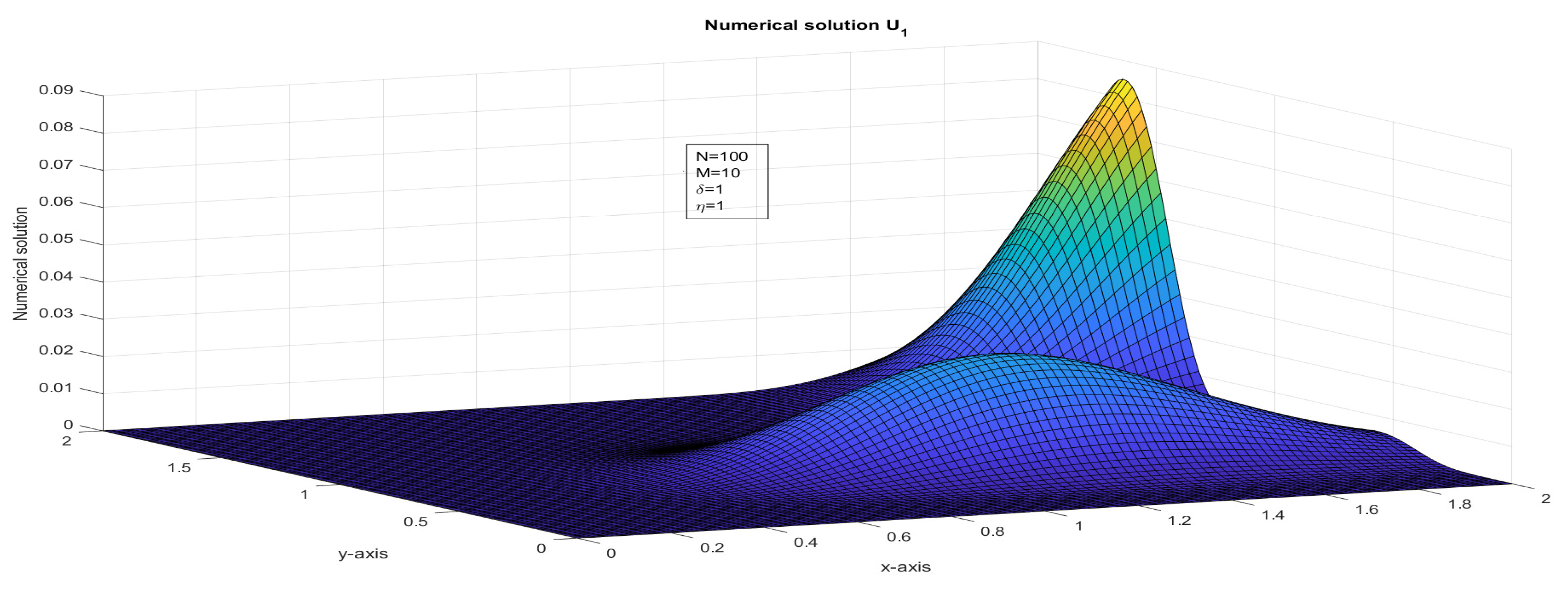
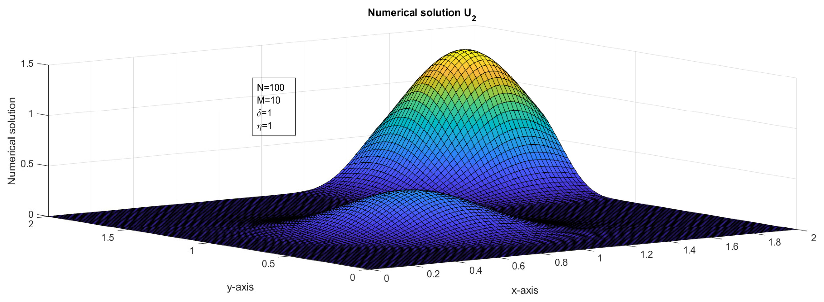
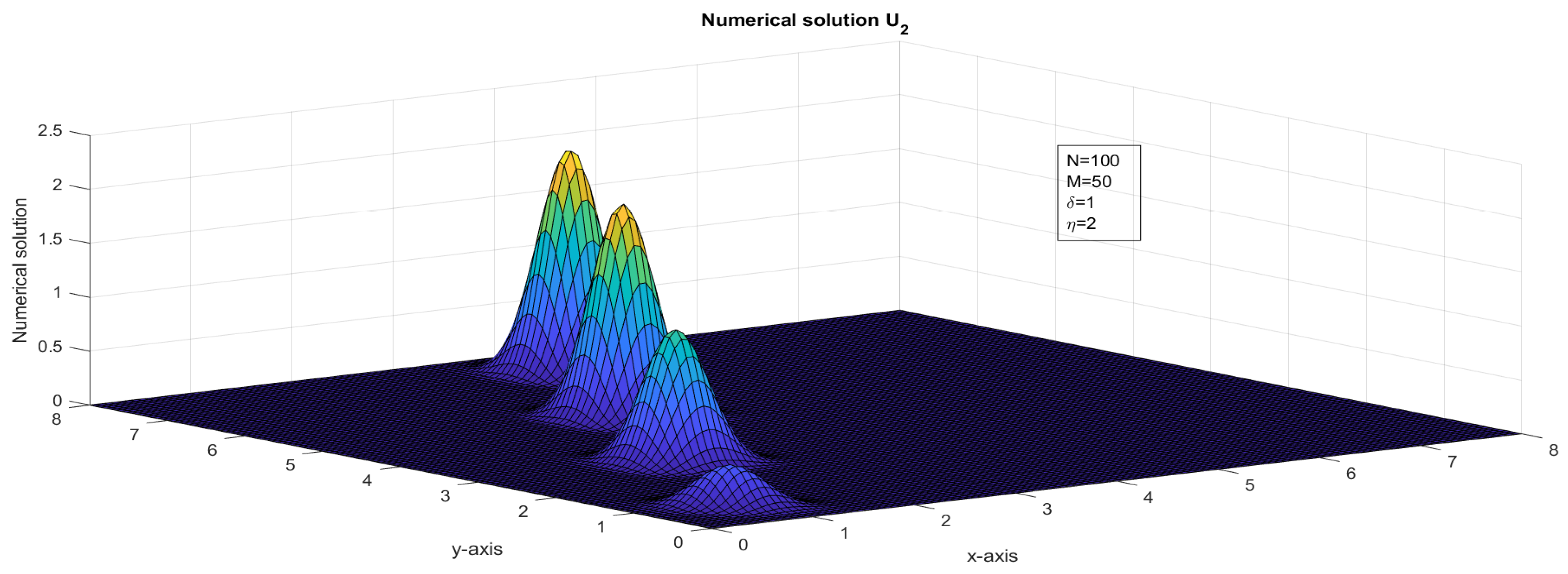
- Case 1:
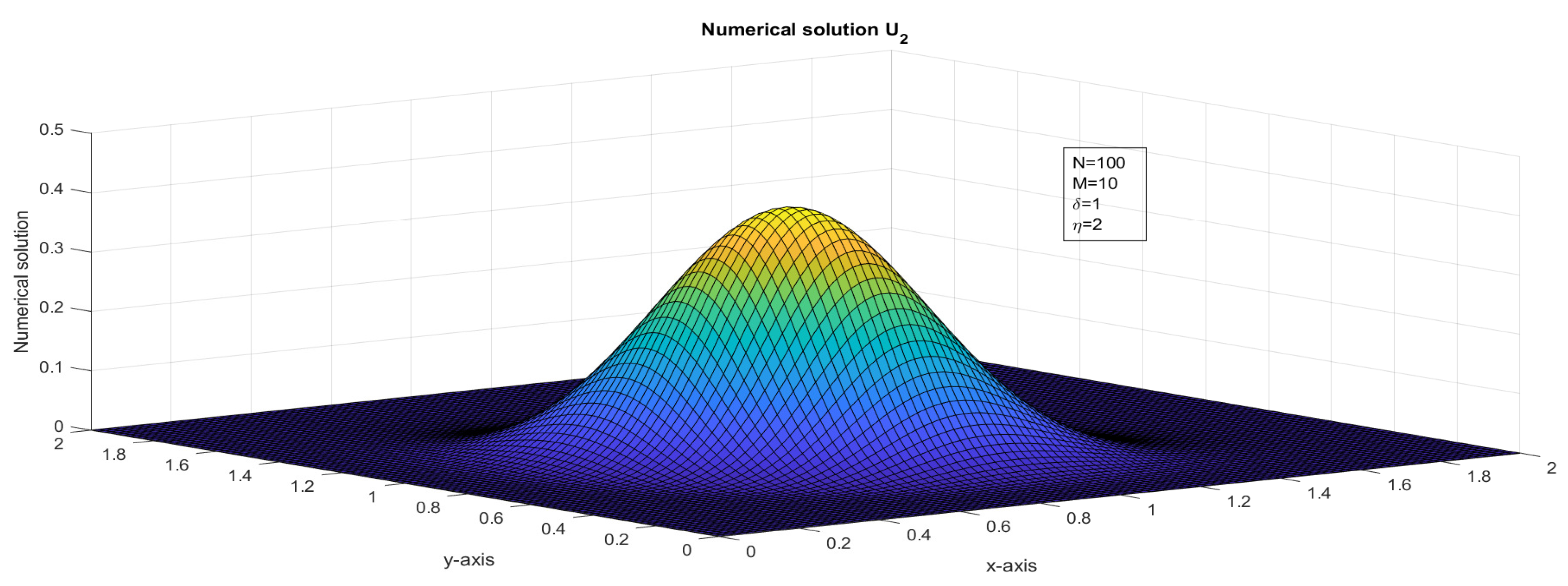
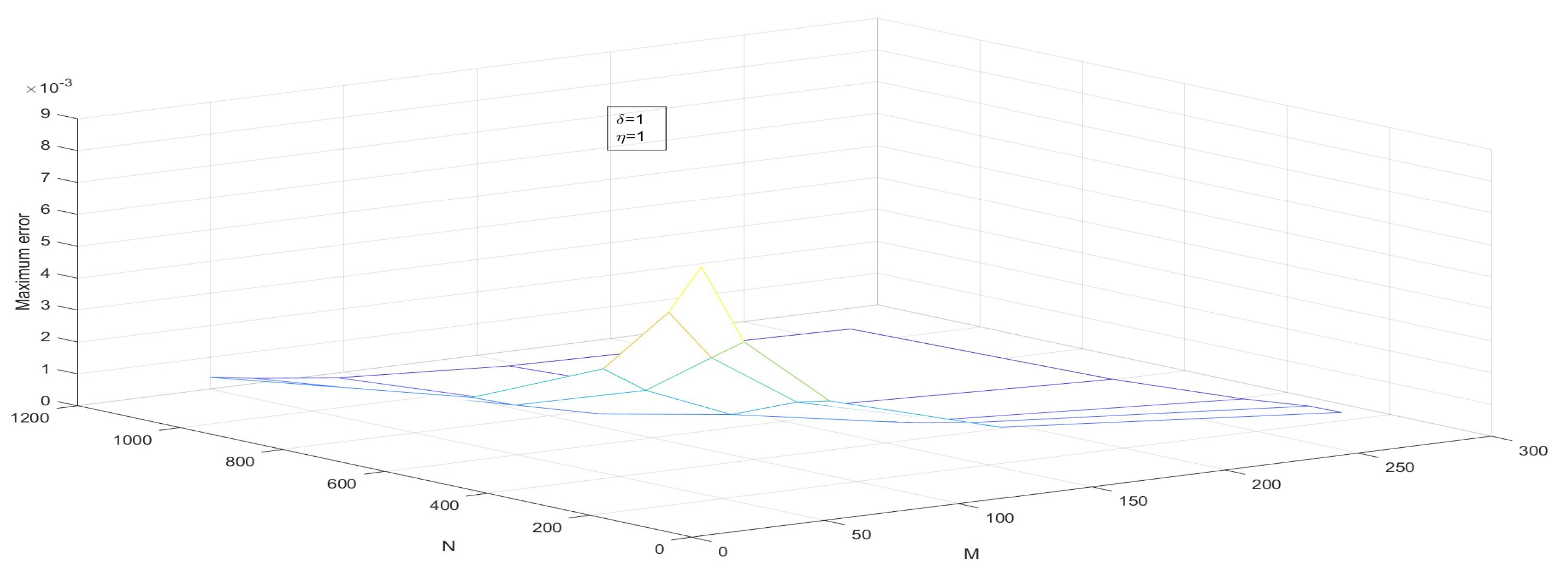
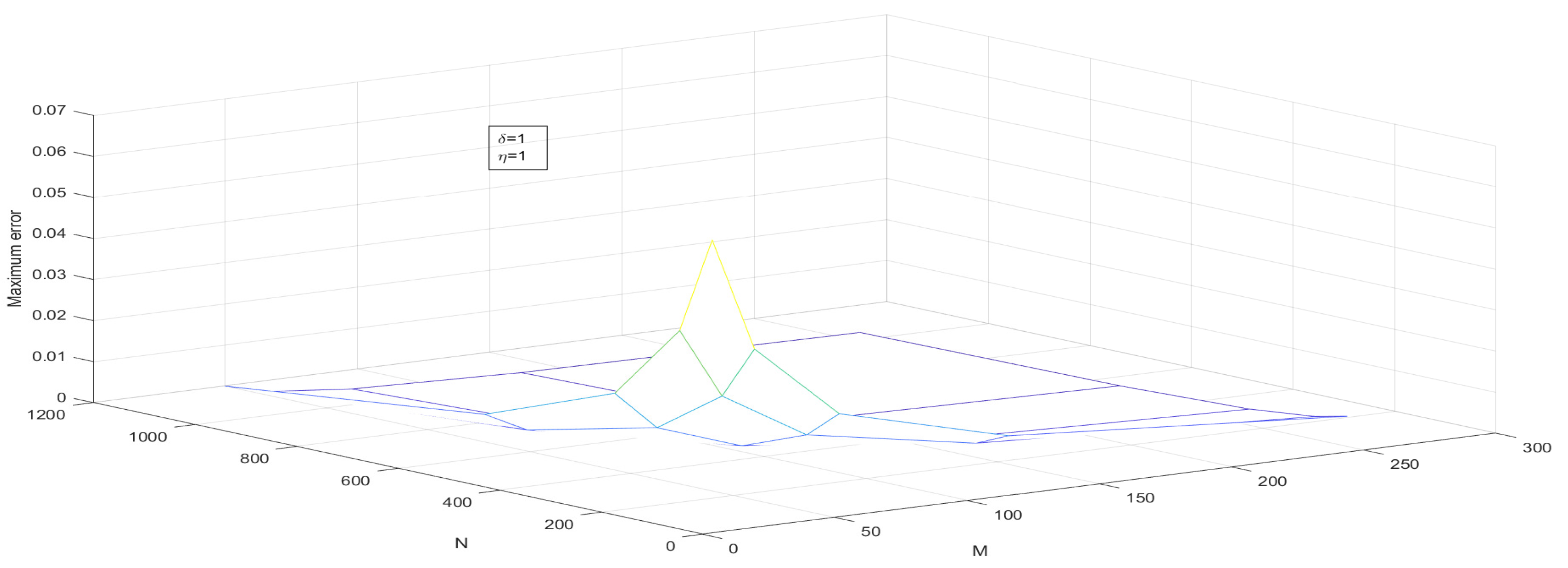
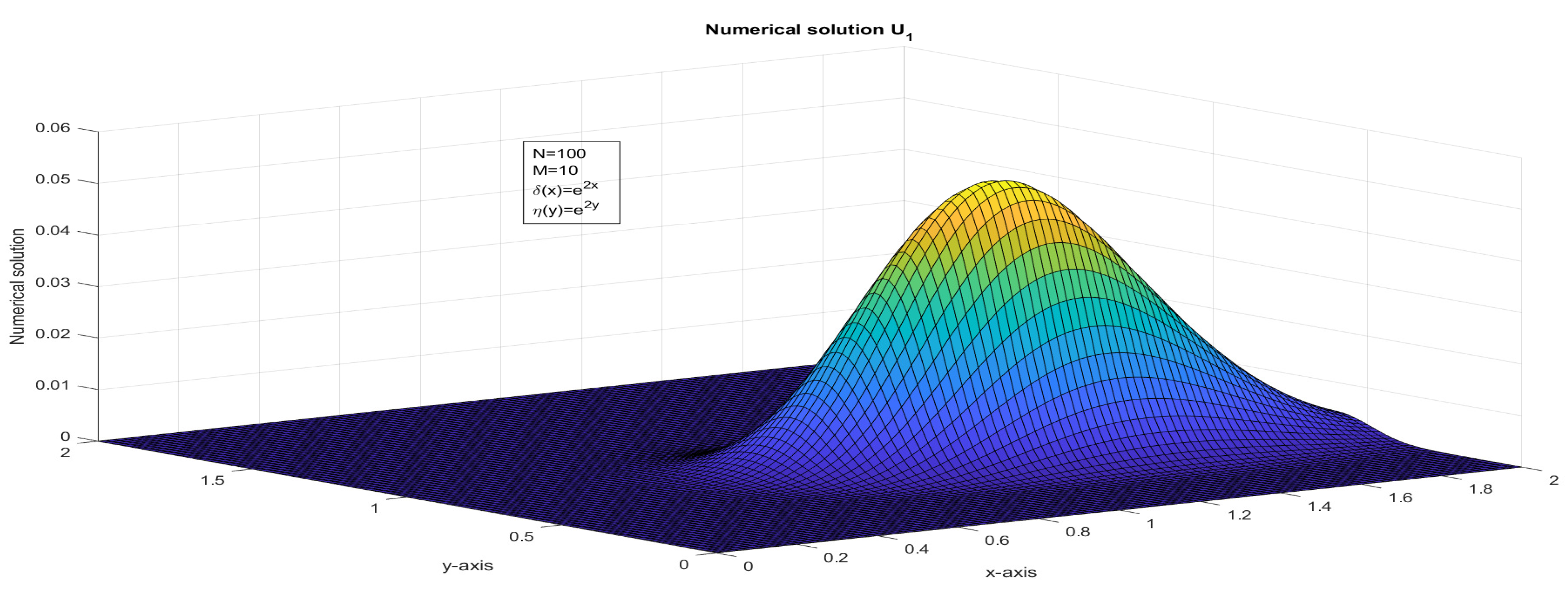
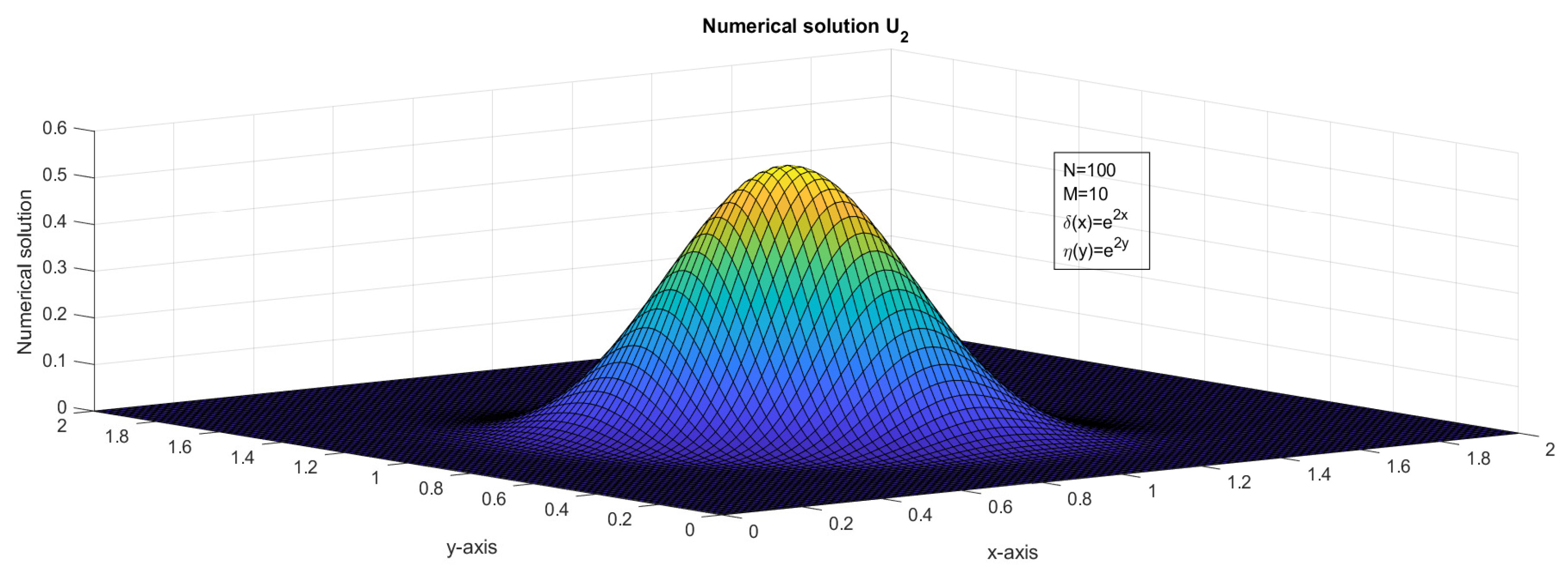
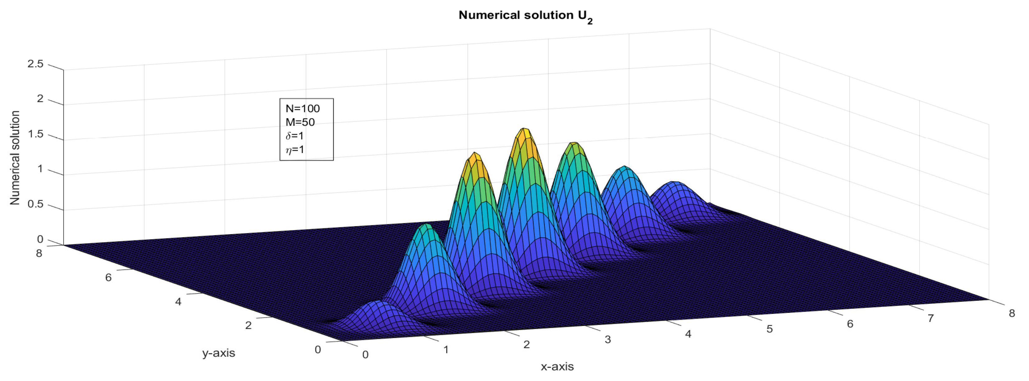
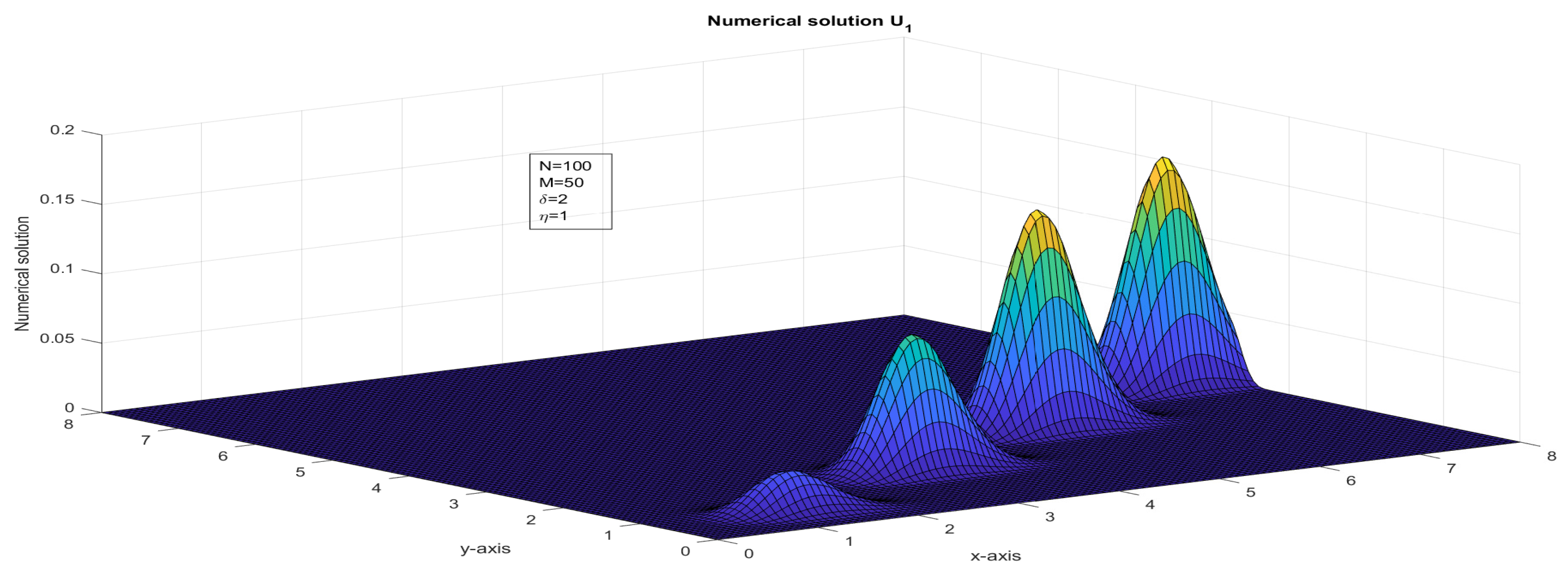
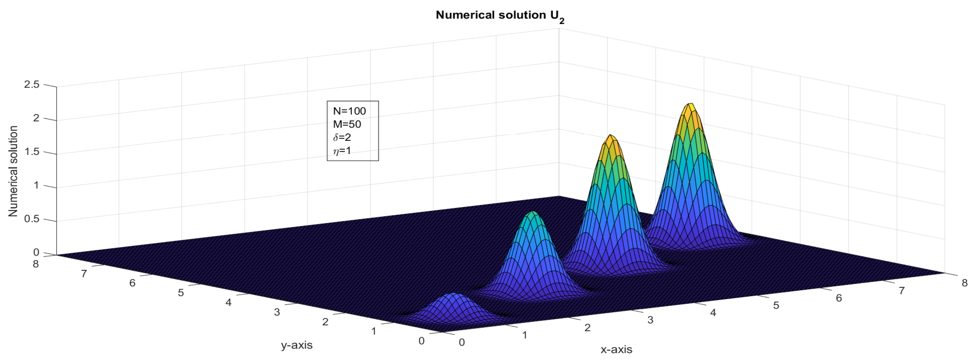
- Assume that . The two-dimensional impulse propagates in the solution due to the presence of the delay term. Numerical solutions are plotted in Figure 1 and Figure 2 and maximum point-wise errors are plotted in Figure 7 and Figure 8. The maximum point-wise errors are given in Table 1 and Table 2. The impulse moves in the forward direction can be found in Figure 11 and Figure 12.
- Case 2:
- Case 3:


| , and N | ||||||
|---|---|---|---|---|---|---|
| M ↓ | 64 | 128 | 256 | 512 | 1024 | |
| 16 | 8.0922 × 10 | 6.4475 × 10 | 4.2323 × 10 | 2.4580 × 10 | 1.3300 × 10 | 8.0922 × 10 |
| 32 | 5.5672 × 10 | 4.8529 × 10 | 3.3899 × 10 | 2.0492 × 10 | 1.1329 × 10 | 5.5672 × 10 |
| 64 | 3.3803 × 10 | 3.1249 × 10 | 2.2935 × 10 | 1.4320 × 10 | 8.0661 × 10 | 3.3803 × 10 |
| 128 | 1.8814 × 10 | 1.7998 × 10 | 1.3716 × 10 | 8.7893 × 10 | 5.0466 × 10 | 1.8814 × 10 |
| 256 | 9.9549 × 10 | 9.7438 × 10 | 7.5796 × 10 | 4.9483 × 10 | 3.1548 × 10 | 9.9549 × 10 |
| 8.0922 × 10 | 6.4475 × 10 | 4.2323 × 10 | 2.4580 × 10 | 1.3300 × 10 | - | |


| , and N | ||||||
|---|---|---|---|---|---|---|
| M ↓ | 64 | 128 | 256 | 512 | 1024 | |
| 16 | 6.8702 × 10 | 4.4892 × 10 | 2.6181 × 10 | 1.4221 × 10 | 7.4248 × 10 | 6.8702 × 10 |
| 32 | 4.0786 × 10 | 2.7619 × 10 | 1.6487 × 10 | 9.0944 × 10 | 4.7898 × 10 | 4.0786 × 10 |
| 64 | 2.2413 × 10 | 1.5539 × 10 | 9.4426 × 10 | 5.2683 × 10 | 2.7922 × 10 | 2.2413 × 10 |
| 128 | 1.1778 × 10 | 8.2741 × 10 | 5.0898 × 10 | 2.8575 × 10 | 1.5196 × 10 | 1.1778 × 10 |
| 256 | 6.0411 × 10 | 4.2797 × 10 | 2.6459 × 10 | 1.4907 × 10 | 7.9392 × 10 | 6.0411 × 10 |
| 6.8702 × 10 | 4.4892 × 10 | 2.6181 × 10 | 1.4221 × 10 | 7.4248 × 10 | - | |


8. Conclusions
Author Contributions
Funding
Data Availability Statement
Conflicts of Interest
References
- Alexander, V.R.; Wu, J. A non-local PDE model for population dynamics with state-selective delay: Local theory and global attractors. J. Comput. Appl. Math. 2006, 190, 99–113. [Google Scholar]
- Al-Mutib, A.N. Stability properties of numerical methods for solving delay differential equations. J. Comput. Appl. Math. 1984, 10, 71–79. [Google Scholar] [CrossRef] [Green Version]
- Bellen, A.; Zennaro, M. Numerical Methods for Delay Differential Equations; Oxford University Press: Oxford, UK, 2003. [Google Scholar]
- Wu, J. Theory and Applications of Partial Functional Differential Equations; Springer: New York, NY, USA, 1996. [Google Scholar]
- Karthick, S.; Mahendran, R.; Subburayan, V. Method of lines and Runge-Kutta method for solving delayed one dimensional transport equation. J. Math. Comput. Sci. 2023, 28, 270–280. [Google Scholar] [CrossRef]
- Tunç, O.; Tunç, C.; Wang, Y. Delay-dependent stability, integrability and boundedeness criteria for delay differential systems. Axioms 2021, 10, 138. [Google Scholar] [CrossRef]
- Tunç, O.; Tunç, C. Solution estimates to Caputo proportional fractional derivative delay integro-differential equations. Rev. Real Acad. Cienc. Exactas Fís. Nat. Ser. A Mat. 2023, 117, 12. [Google Scholar] [CrossRef]
- Stein, R.B. A theoretical analysis of neuronal variability. Biophys. J. 1965, 5, 173–194. [Google Scholar] [CrossRef] [Green Version]
- Stein, R.B. Some models of neuronal variability. Biophys. J. 1967, 7, 37–68. [Google Scholar] [CrossRef] [Green Version]
- Sharma, K.K.; Singh, P. Hyperbolic partial differential-difference equation in the mathematical modelling of neuronal firing and its numerical solution. Appl. Math. Comput. 2008, 201, 229–238. [Google Scholar]
- Singh, P.; Sharma, K.K. Finite difference approximations for the first-order hyperbolic partial differential equation with point-wise delay. Int. J. Pure Appl. Math. 2011, 67, 49–67. [Google Scholar]
- Singh, P.; Sharma, K.K. Numerical solution of first-order hyperbolic partial differential-difference equation with shift. Numer. Methods Partial Differ. Equ. 2010, 26, 107–116. [Google Scholar] [CrossRef]
- Karthick, S.; Subburayan, V. Finite Difference Methods with Interpolation for First-Order Hyperbolic Delay Differential Equations. Springer Proc. Math. Stat. 2021, 368, 147–161. [Google Scholar]
- Karthick, S.; Subburayan, V. Finite difference methods with linear interpolation for solving a coupled system of hyperbolic delay differential equations. Int. J. Math. Model. Numer. Optim 2022, 12, 370–389. [Google Scholar] [CrossRef]
- Karthick, S.; Subburayan, V.; Agrwal, R.P. Stable Difference Schemes with Interpolation for Delayed One-Dimensional Transport Equation. Symmetry 2022, 14, 1046. [Google Scholar]
- Fridmana, E.; Orlov, Y. Exponential stability of linear distributed parameter systems with time-varying delays. Automatica 2009, 45, 194–201. [Google Scholar] [CrossRef]
- Smith, G.D. Numerical Solution of Partial Differential Equations: Finite Difference Methods; Oxford University Press: Oxford, UK, 1985. [Google Scholar]
- Strikwerda, J.C. Finite Difference Schemes and Partial Differential Equations; SIAM: Philadelphia, PA, USA, 2004. [Google Scholar]
- Islam, S.; Alam, M.; Al-Asad, M.; Tunç, C. An analytical technique for solving new computational of the modified Zakharov-Kuznetsov equation arising in electrical engineering. J. Appl. Comput. Mech. 2021, 7, 715–726. [Google Scholar]
- Alam, M.N.; Tunc, C. An analytical method for solving exact solutions of the nonlinear Bogoyavlenskii equation and the nonlinear diffusive predator–prey system. Alex. Eng. J. 2016, 55, 1855–1865. [Google Scholar] [CrossRef] [Green Version]
- Jiwari, R. Lagrange interpolation and modified cubic B-spline differential quadrature methods for solving hyperbolic partial differential equations with Dirichlet and Neumann boundary conditions. Comput. Phys. Commun. 2015, 193, 55–65. [Google Scholar] [CrossRef]
- Jiwari, R.; Pandit, S.; Mittal, R. A differential quadrature algorithm to solve the two dimensional linear hyperbolic telegraph equation with Dirichlet and Neumann boundary conditions. Appl. Math. Comput. 2012, 218, 7279–7294. [Google Scholar] [CrossRef]
- Pandit, S.; Kumar, M.; Tiwari, S. Numerical simulation of second-order one dimensional hyperbolic telegraph equation. Comput. Phys. Commun. 2015, 187, 83–90. [Google Scholar] [CrossRef]
- Protter, M.H.; Weinberger, H.F. Maximum Principles in Differential Equations; Springer Science and Business Media: New York, NY, USA, 2012. [Google Scholar]
- Mizohata, S.; Murthy, M.V.; Singbal, B.V. Lectures on Cauchy Problem; Tata Institute of Fundamental Research: Bombay, India, 1965; Volume 35. [Google Scholar]
- Peaceman, D.W.; Rachford, H.H. The numerical solution of parabolic and elliptic differential equations. SIAM J. Comput. 1955, 3, 28–41. [Google Scholar] [CrossRef]
- Thomas, B.G.; Samarasekera, I.V.; Brimacombe, J.K. Comparison of numerical modeling techniques for complex, two-dimensional, transient heat-conduction problems. Metall. Trans. B 1984, 15, 307–318. [Google Scholar] [CrossRef] [Green Version]
- Araújo, A.; Neves, C.; Sousa, E. An alternating direction implicit method for a second-order hyperbolic diffusion equation with convection. Appl. Math. Comput. 2014, 239, 17–28. [Google Scholar] [CrossRef] [Green Version]
- Clavero, C.; Jorge, J.C.; Lisbona, F. A uniformly convergent scheme on a nonuniform mesh for convection–diffusion parabolic problems. J. Comput. Appl. Math. 2003, 154, 415–429. [Google Scholar] [CrossRef] [Green Version]
- Clavero, C.; Jorge, J.C.; Lisbona, F.; Shishkin, G.I. An alternating direction scheme on a nonuniform mesh for reaction-diffusion parabolic problems. IMA J. Numer. Anal. 2000, 20, 263–280. [Google Scholar] [CrossRef] [Green Version]
- Majumdar, A.; Natesan, S. Alternating direction numerical scheme for singularly perturbed 2D degenerate parabolic convection-diffusion problems. Appl. Math. Comput. 2017, 313, 453–473. [Google Scholar] [CrossRef]
- Avudai Selvi, P.; Ramanujam, N. A parameter uniform difference scheme for singularly perturbed parabolic delay differential equation with Robin type boundary condition. Appl. Math. Comput. 2017, 296, 101–115. [Google Scholar] [CrossRef]
- Subburayan, V.; Ramanujam, N. An asymptotic numerical method for singularly perturbed convection-diffusion problems with a negative shift. Neural Parallel Sci. Comput. 2013, 21, 431–446. [Google Scholar]
- Walter, A. Strauss, Partial Differential Equations an Introduction; John Wiley & Sons, Inc.: New York, NY, USA, 2008. [Google Scholar]
- Subburayan, V.; Natesan, S. Parameter Uniform Numerical Method for Singularly Perturbed 2D Parabolic PDE with Shift in Space. Mathematics 2022, 10, 3310. [Google Scholar] [CrossRef]
- Zadorin, A.I. Approaches to constructing two-dimensional interpolation formulas in the presence of boundary layers. J. Phys. Conf. Ser. 2022, 2182, 012036. [Google Scholar] [CrossRef]
- Miller, J.J.H.; O’Riordan, E.; Shishkin, G.I. Fitted Numerical Methods for Singular Perturbation Problems: Error Estimates in the Maximum Norm for Linear Problems in One and Two Dimensions; World Scientific: Singapore, 2012. [Google Scholar]
- Varah, J.M. A lower bound for the smallest singular value of a matrix. Linear Algebra Its Appl. 1975, 11, 3–5. [Google Scholar] [CrossRef] [Green Version]
- Agarwal, R.P.; Chow, Y.M. Finite-difference methods for boundary-value problems of differential equations with deviating arguments. Comput. Method. Appl. Math. 1986, 12, 1143–1153. [Google Scholar] [CrossRef] [Green Version]
- Jain, R.K.; Agarwal, R.P. Finite difference method for second order functional differential equations. J. Math. Phys. Sci. 1973, 7, 301–316. [Google Scholar]
Disclaimer/Publisher’s Note: The statements, opinions and data contained in all publications are solely those of the individual author(s) and contributor(s) and not of MDPI and/or the editor(s). MDPI and/or the editor(s) disclaim responsibility for any injury to people or property resulting from any ideas, methods, instructions or products referred to in the content. |
© 2023 by the authors. Licensee MDPI, Basel, Switzerland. This article is an open access article distributed under the terms and conditions of the Creative Commons Attribution (CC BY) license (https://creativecommons.org/licenses/by/4.0/).
Share and Cite
Sampath, K.; Veerasamy, S.; Agarwal, R.P. Fractional-Step Method with Interpolation for Solving a System of First-Order 2D Hyperbolic Delay Differential Equations. Computation 2023, 11, 57. https://doi.org/10.3390/computation11030057
Sampath K, Veerasamy S, Agarwal RP. Fractional-Step Method with Interpolation for Solving a System of First-Order 2D Hyperbolic Delay Differential Equations. Computation. 2023; 11(3):57. https://doi.org/10.3390/computation11030057
Chicago/Turabian StyleSampath, Karthick, Subburayan Veerasamy, and Ravi P. Agarwal. 2023. "Fractional-Step Method with Interpolation for Solving a System of First-Order 2D Hyperbolic Delay Differential Equations" Computation 11, no. 3: 57. https://doi.org/10.3390/computation11030057