Feature Selection Using New Version of V-Shaped Transfer Function for Salp Swarm Algorithm in Sentiment Analysis

Abstract

(1) Background: Feature selection is the biggest challenge in feature-rich sentiment analysis to select the best (relevant) feature set, offer information about the relationships between features (informative), and be noise-free from high-dimensional datasets to improve classifier performance. This study aims to propose a binary version of a metaheuristic optimization algorithm based on Swarm Intelligence, namely the Salp Swarm Algorithm (SSA), as feature selection in sentiment analysis. (2) Methods: Significant feature subsets were selected using the SSA. Transfer functions with various types of the form S-TF, V-TF, X-TF, U-TF, Z-TF, and the new type V-TF with a simpler mathematical formula are used as a binary version approach to enable search agents to move in the search space. The stages of the study include data pre-processing, feature selection using SSA-TF and other conventional feature selection methods, modelling using K-Nearest Neighbor (KNN), Support Vector Machine, and Naïve Bayes, and model evaluation. (3) Results: The results showed an increase of 31.55% to the best accuracy of 80.95% for the KNN model using SSA-based New V-TF. (4) Conclusions: We have found that SSA-New V3-TF is a feature selection method with the highest accuracy and less runtime compared to other algorithms in sentiment analysis.

1. Introduction

Social media is the most significant contributor to data growth [1]. The increasing use of social media has created many opportunities for people to express their opinions and ideas [2]. Through social media, everyone can express their opinion about many things, such as products, celebrities and services [3]. Social media, especially Twitter, is now becoming more popular among people as it provides a direct platform for users to express their views on any topic, show emotions or sentiments towards any event [4], and also can express user opinion on any topic in the form of tweets [5].

Sentiment analysis (SA) is a process that aims to determine the results of a content assessment of text datasets (documents, sentences, paragraphs, etc.) so that the contents can be classified into positive, negative or neutral [6]. SA serves to find the general emotion of social media posts [7]. SA has changed from interpreting online textual output analysis to understanding social media contextual text, for example, from Twitter. Several SA approaches include lexicon-based approaches, machine learning (ML) or a combination of the two (hybrid) [8].

SA is a difficult task, especially when dealing with very large data sets, because the techniques behind SA produce high-dimensional, unstructured and feature-rich representations [9]. The dimension is the number of features of data. Selecting or removing some features manually is vulnerable to bias because of the ability of a person in a particular domain. Feature selection is a fundamental task in implementing an effective SA [10]. Effective SA means that the number of features is reduced so that the dimensional space is reduced, as well as having an impact on increasing classification accuracy and the computational process tends to be fast [11].

One of the automation techniques to reduce high-dimensional space in sentiment analysis using machine learning is the feature selection technique (FST) [12]. The FST is able to reduce the original feature set and remove features that are irrelevant for classification [13]. Feature selection is carried out to select the best (relevant) set of features, offers a lot of information about the relationships between features (informative) and is noise-free from high-dimensional datasets to improve classifier performance [14]. The FST is very important for SA because smaller dimensions of the data set will reduce the running time of the machine learning implementations and increase the performance of the classifier process [15]. SA using the FST is able to reduce more than 70% of all features, there is an 84% increase in classifier execution time due to the reduced amount of data resulting in reduced computation time, and it increases accuracy by about 8%, from 76% to 84% [11]. Based on the previous study, SA using the FST resulted in a reduced number of features, increased computation time and better classification accuracy than without the FST [10,16].

The optimization algorithm for the FST has advantages over the FST without optimization because of the ability to select optimal features or approach optimal subsets of features in an acceptable amount of time [17]. There are many metaheuristic algorithms for feature selection. The metaheuristic algorithm is a further development of the heuristic algorithm, which can perform better [18]. Modern metaheuristic algorithms inspired by nature, whose classification is population-based and trajectory-based, are almost guaranteed to work well for many difficult optimization problems [18], one of them for the FST [19]. Optimization algorithms with a metaheuristic approach have been widely proposed in previous studies to improve the FST performance in an effective SA [10]. Several metaheuristic algorithms that are popularly used as an FST in SA include the genetic algorithm (GA) [20], ant colony optimization (ACO) [19,21,22,23], and particle swarm optimization (PSO) [24,25,26]. The GA has advantages such as the FST over SA, which are not too complex, are easier to use and the ability to solve optimization problems based on the chromosomal approac [27]. However, the GA has drawbacks, namely when faced with large feature sizes that can affect the ability to obtain optimal solutions [23]. In addition, when the overall solution has several populations, the GA does not continuously reduce the global optimum, so it takes a long time to process [27]. ACO as an FST in SA has advantages, including having the ability to perform optimally to select optimal and fast feature subsets in convergence [23]. Even so, ACO has drawbacks in the processing time, which may be affected by dimensions (total features) and data size [23]. PSO has the advantage of having strong exploratory capabilities because it is a gradual search process to approach the optimal solution [26], but it has the same drawback as the GA and ACO, namely that the processing time can also be extended because it is easy to get stuck in partial optimal [25].

The salp swarm algorithm (SSA) has been proposed as an optimization algorithm for the FST [18,19,20]. The SSA algorithm, first proposed in 2017, is a bio-inspired metaheuristic optimization algorithm based on swarm intelligence [28]. Feature selection using the SSA obtained the highest accuracy, of 100% and the lowest running time, of 0.08 min, for all real biomedical datasets compared to other feature selections using different evolution and particle swarm optimization [29]. In the study on increasing the machine learning-based network anomaly detection, the SSA has better accuracy performance than other optimization algorithms, reaching 99% as a feature selection optimization algorithm for detecting networks [30]. Based on the ability to balance exploration and exploitation, the SSA is able to perform better than other conventional swarm algorithms for feature selection on biomedical and clinical data, with the highest accuracy reaching 94.23% in the k-nearest neighbor classification algorithm [31]. Based on previous studies, the application of the SSA as an FST for the domain of sentiment analysis still needs to be improved. The application of the SSA as an FST in sentiment analysis is the first time it has been carried out for Arabic language datasets, with the highest accuracy results reaching 80.80% after the SSA was combined with the S-shaped transfer function [32]. The accuracy obtained from the ability of the SSA as an FST in the domain of sentiment analysis still has gaps for running time in the process. The running time that occurs is still relatively long compared to other swarm algorithms, namely particle swarm optimization. In addition, there is no application of the SSA as an FST in the domain of sentiment analysis using various languages such as English.

The transfer function (TF) plays a role in the optimizer binarization process for mapping the search space, optimizing the convergence speed and accuracy of the optimization algorithm [23,24], including the SSA. In previous studies, apart from the SSA, the transfer function has been successfully applied to metaheuristic optimization algorithms for feature selection, such as ant lion, which implements the S-shaped and V-shaped transfer functions, which obtain the highest accuracy, reaching 97.40% [33]. As an optimization algorithm for feature selection, the competitive swarm optimizer algorithm also produces a high classification accuracy of 100% and low computational costs [34]. Other metaheuristic optimization algorithms, such as the equilibrium optimizer, produce spectacular accuracy, reaching 100%, as a feature selection optimization algorithm with fewer features using the U-shaped transfer functions approach [35]. The transfer function can improve the performance of the optimization algorithm for feature selection in machine learning classification modelling. There are 21 types of TF to convert continuous SSA into binary, namely S-TF (which has four S-type variants), V-TF (which has four V-type variants), X-TF [36] (which has two X-type variants), U-TF [37] (which has three U-type variants), and Z-TF [38,39] (which has four Z-type variants). In this study, a new version of V-TF (four new versions of V-type variants) with a simpler mathematical formula is also included as a binary version approach to enable search agents to move in the search space. Salps in binary SSA are allowed to move in a finite direction bounded by 0 and 1, so it is very suitable for TF to be used to define the probability of updating elements in a subset of features (solutions) to 1 or 0 [40].

This study aims to compare the performance of several types of transfer functions (TF) in the implementation of the salp swarm algorithm (SSA) in creating sentiment classification models of Twitter data. The TF types are S-TF, V-TF, X-TF, U-TF and Z-TF, as well as a new version of V-TF with a simpler mathematical formula. The classification model was built by applying three machine learning algorithms, namely k-nearest neighbor, naïve Bayes and support vector machine. The main contributions in this study include (1) proposing optimization of the salp swarm algorithm (SSA) by modifying the SSA and transfer function (TF) optimization algorithms using various types of TFs, namely S-TF, V-TF, X-TF, U- TF and Z-TF, as well as V-TF with a simpler mathematical formula into the salp swarm algorithm transfer function (SSA-TF) so that convergence in the feature selection process is faster, optimal and the resulting feature results are informative, relevant and increase classification accuracy results in sentiment analysis; (2) the second contribution is to apply the proposed algorithm to the English sentiment analysis problem. To validate our proposed approach, we compared it with well-known bio-inspired optimizers such as particle swarm optimization (PSO) and the ant lion optimizer (ALO) algorithm.

The structure of this paper is as follows: The background of the salp swarm algorithm (SSA) is presented in Section 2. The materials and methods used in this study are presented in Section 3. The improved salp swarm algorithm using the transfer function (SSA-TF) is presented in Section 4. The application of the SSA-TF in feature selection in sentiment analysis is presented in Section 5. Section 6 presents and discusses the experimental results of this study. Finally, Section 7 presents conclusions.

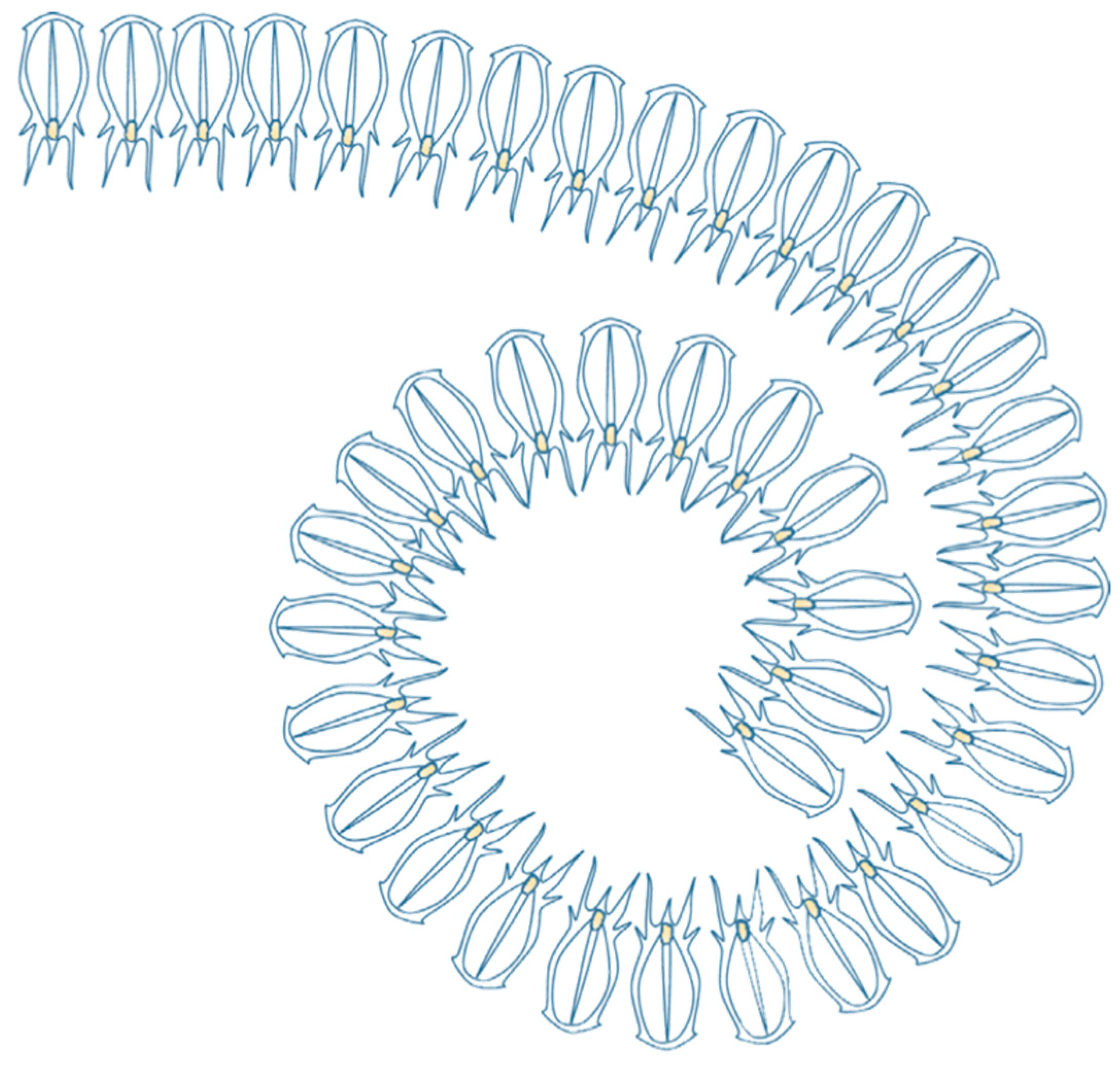
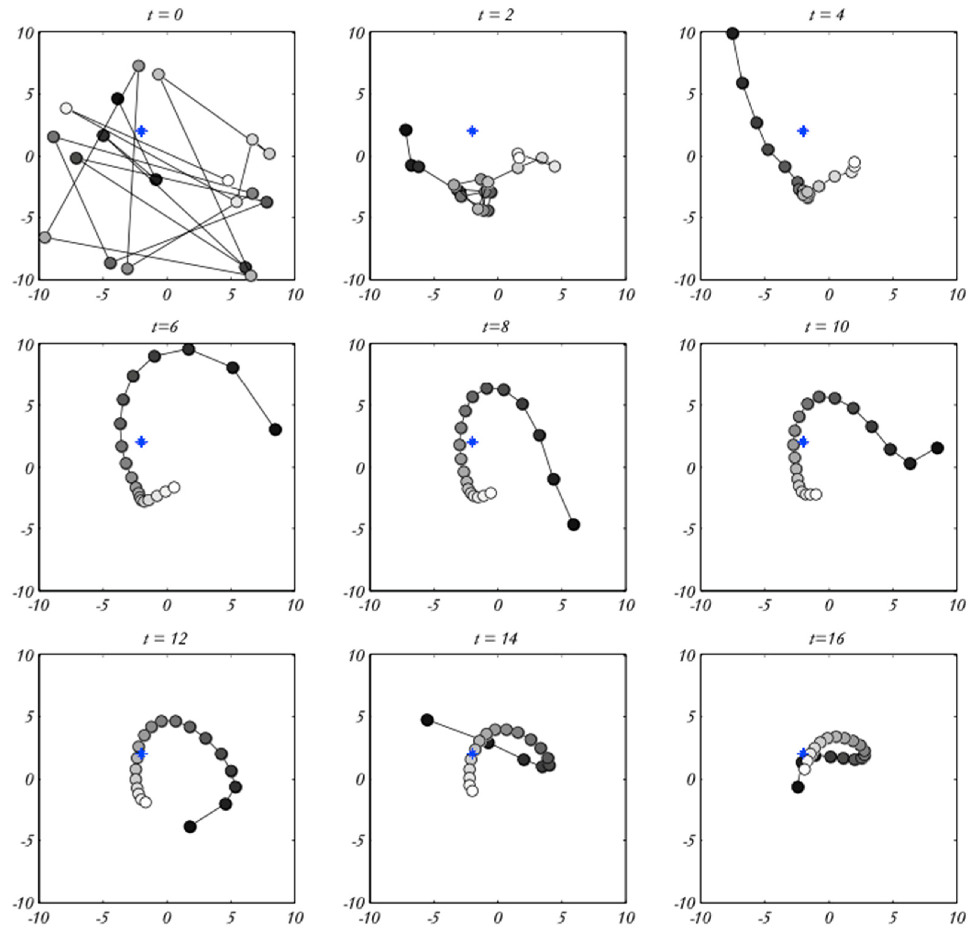
2. Salp Swarm Algorithm (SSA)

The Salp Swarm Algorithm (SSA) was introduced by [28] in 2017. The SSA is included in the category of swarm-based algorithms with a metaheuristic approach. The SSA is a swarm intelligence optimization algorithm that simulates the movement behavior of salp population chains in the sea [41]. Optimization techniques mainly aim to find the best decision (problem solution) by optimizing the objective function or fitness function. The objective of decision-making is to determine the optimal value of several available alternatives. The optimization process results in the choice of a decision or the best value of all choices [42]. Illustrations of individual salp animals, as well as salp chains and the leader and follower concepts, can be seen in Figure 1 and Figure 2 [28].

The SSA simulates a salp-swarming mechanism when searching for food in the ocean [39]. On the ocean floor, salps usually form shoals known as salp chains. In the SSA algorithm, the leader is the salp at the front of the chain and whatever is left of the salp is called the follower. As with other swarm-based techniques, salp positions are defined in an s-dimensional search space, where s is the number of variables from the given problem. Therefore, the positions of all salps are stored in a two-dimensional matrix called $x$. It is also assumed that there is a food source called P in the search space as the target of the swarm. The movement of the salp herd chain in the search space can be seen in Figure 3 [28].

Simulation is needed to see the SSA mathematical model [28]. Twenty salps were randomly placed in search chambers with fixed or immobile food sources. The position of the salp chain and the history of each salp is illustrated in Figure 3. The blue dots on the figure indicate the position of the food source, and the darkest black circle contains the salp. Follower salps are coloured grey based on their position in the salp chain concerning the salp leader. Based on Figure 3, it can be seen the various movement behaviours of the salp chain for nine successive iterations. Salp sets can be formed and moved using the proposed equation according to the algorithm effectively after the first iteration. The leading salp will change its position around the food source, and then the follower salp gradually follows it throughout the iteration. Simulations using 2D space show that the model can display the behaviour of the salp swarm algorithm in n-dimensional space.

A group of $X$ salps out of n are represented by a two-dimensional matrix in the SSA algorithm, as shown in the mathematical Equation (1) [28]. The food source that the salps chain is designed to reach is symbolized by the letter $F$ in the search space.

$$X_i=\left[\begin{array}{cccc}{x}_1^1& x_2^1& \cdots & x_d^1\\ x_1^2& x_2^2& & x_d^2\\ ⋮& & \ddots & ⋮\\ x_1^n& x_2^n& \cdots & x_d^n\end{array}\right]$$

(1)

Based on the SSA model (1), then the mathematical model for SSA [28] is given as follows:

$$x_{j }^1=\{\begin{array}{c}{F}_j+c_{1 }+\left(\left(u{b}_j-l{b}_{j }\right)c_2+l{b}_{j }\right) c_3\ge 0\\ F_j-c_{1 }+\left(\left(u{b}_j-l{b}_{j }\right)c_2+l{b}_{j }\right) c_3<0\end{array}$$

(2)

Based on the leader position formula (the salp that is at the top) is shown in $x_{j }^1$. The position of the food source in the j dimension is indicated by $F_j$. The upper limit of the $j$ dimension is indicated by $u{b}_j$. the lower bound of the $j$ dimension is indicated by $l{b}_j$. random numbers are assigned to $c_1$, $c_2$ and $c_3$. The coefficient $c_1$ is an important parameter in SSA because it provides a balance between exploration and exploitation capabilities.

$$c_1=2e^{-{(\frac{4l}{L})}^2}$$

(3)

The current iteration is called $l$ and the maximum number of iterations is $L$. The random numbers generated uniformly in the interval [1, 0] are parameters $c_2$ and $c_3$. In the process, these parameters determine the next position in the jth dimension leading to positive infinity or negative infinity and the step size. The follower positions are updated with the following (Newton′s laws of motion [43]) equation:

$$x_{j }^i=\frac{1}{2}a{t}^2+v_0{}^t$$

(4)

If $i\ge 2$, $x_{j }^i$ denotes the salp position of the $i$th follower in the $j$th dimension, $t$ shows the time, $v_0$ indicates the initial speed and $a=\frac{v_{final}}{v_0}$ dimana $v=\frac{x-x_0}{t}$. Because iterations indicate time in optimization, the conflict between iterations is 1, then by considering $v_0=0$, this equation can be declared as follows:

$$x_{j }^i=\frac{1}{2}(x_{j }^i+x_{j }^{i-1})$$

(5)

The position of the $i$th salp follower at $j$th is indicated by $x_{j }^i$, where $i\ge 2$. The salp chain can be simulated using Equations (2) and (5). Based on this formula, $x_{j }^i$ is the $i$th leader position in the $j$th dimension, $F_j$ is the position of the food source in the $j$th dimension, $u_{bj}$ is the upper limit of the $j$th dimension, $l_{bj}$ is the lower limit of the $j$th dimension, $c_1$, $c_2$ and $c_3$ are random variables that are generated uniformly in the interval. The salp swarm algorithm (SSA) pseudocode is presented in Algorithm 1 [28].

Algorithm 1. Salp Swarm Algorithm

Input parameter: Population Size, Number of Iterations, Min Values, Max Values

(1) Initialize the salp population $x_i$ ($i=1, 2, 3, \dots , n)$considering ub and lb

(2) while (end condition is not satisfied) do

(3) calculate the fitness of each search agent (salp)

(4) $F=$ the best search agent

(5) update $c_1$ by Equation (3)

(6)  for each salp ($x_i$)

(7)    if $\left(i==1\right)$

(8)       Update the position of the leading salp by Equation (2)

(9)    else (10)       Update the position of the follower salp by Equation (5) (11)    end (12)  end

(13) Amend the salps based on the upper and lower bounds of variables

(14) end

(15) return F

Output: Global best solution

The SSA has advantages, including when the SSA is combined with other algorithms: it produces excellent accuracy values, the process of getting the best solution tends to be fast, and the SSA is suitable for various types of optimization problems [42]. In addition, the SSA is an efficient global search scheme, suitable for a wide search space and it has good search environment characteristics, such as adaptability, robustness, scalability and reliability in achieving goals, it has excellent feasibility and efficiency in generating global optima, as well as a small possibility of being trapped in optimal local conditions. However, the SSA needs to improve in the FST process; namely, it is binary, so it is less optimal and tends to be slow to reach convergence in the feature selection process or can even go down to local optima [24,33].

3. Materials and Methods

This study uses benchmark sentiment analysis (Twitter) data, namely the Twitter US Airline Sentiment, available at https://www.kaggle.com/datasets/crowdflower/twitter-airline-sentiment (accessed on 31 August 2021) [44]. These data contained expressions posted on Twitter by travelers about US airlines in February 2015. To build a classification of sentiment towards US airlines by applying the SSA, this study consisted of several stages:

• Text Pre-Processing

Text pre-processing is done to clean text data so that the data will then be ready to be modelled for the next process or stage. The preprocessing techniques used include:

a.

Tokenization

At this stage, words, symbols, phrases and other important entities (which are referred to as tokens) are separated from a text for further analysis. Tokenization breaks down a set of characters in a text (sentence) into units of words. In addition, at this stage, features or words are selected that are not valid words. In this case, we removed all punctuation marks and any entities that are not letters.

b.

Transform Case

In this step, the letters are changed from uppercase to lowercase for all words in the sentence.

c.

Filter Stopword

The important words are taken from the token results. Here, we use the stoplist algorithm (discarding less important words) or wordlist (saving important words).

d.

Stopword Removal

This stage removes less important words, such as conjunctions or articles, namely “that”, “the”, “is”, “are” and so on.

e.

Generate N-grams

An N-gram is a combination of adjectives that often appear to indicate a sentiment of text data, which only consists of one word. Bigrams consist of two words and trigrams contain three words. This study used the type of trigram token.

f.

Stemming

The stemming technique was needed in addition to minimizing the number of different terms of a document. Stemming is also used for grouping other words that have a base word and a similar meaning but have a different form because they get different affixes.

2.

Data Partition

The data were divided into two divisions: training data and testing data. The training data were used to train the algorithm in finding a suitable model, while the testing data were used to test and determine the performance of the model. At this stage, the training data containing the set of features were trained using the SSA as the feature selection technique. At the same time, the test data were used to evaluate the model.

3.

Salp Swarm Algorithm (SSA) implementation

The SSA was applied as an optimization algorithm to training data to select features optimally. At this stage, several forms of transfer functions were implemented, namely the S-shaped TF [45] (which has four S-type variants in Equations (6)–(9)), V-Shaped TF [45] (which has four V-type variants in Equations (11)–(14)), X-TF [36] (which has two X-type variants in Equations (16) and (17)), U-TF [37] (which has three U-type variants in Equations (19)–(21)), and Z-TF [38,42] (which has four Z-type variants in Equations (23)–(26)). In this study, a new version of V-TF in Equations (28)–(31) with a simpler mathematical formula was also included as a binary version approach to enable search agents to map the search space and optimize the convergence speed and accuracy of the optimization algorithm. To validate our proposed approach, we compared it with well-known bio-inspired optimizers such as particle swarm optimization (PSO) and the ant lion optimizer (ALO) algorithm.

4.

Develop Classification Models

The classification algorithms used were the k-nearest neighbor, support vector machine and naïve Bayes algorithm. Those algorithms have been very popularly used in studies on sentiment analysis, text classification or opinion gathering. This study utilized the Python programming language to process data and develop models.

5.

Model Evaluation

Classifier evaluation was conducted using ten-fold validation. The confusion matrix was calculated to evaluate the models. Model performance was evaluated based on accuracy, precision, recall, F1-score, time processing and feature probability.

4. Improved of Salp Swarm Algorithm Using Transfer Function (SSA-TF)

The development of the salp swarm algorithm using the transfer function (SSA-TF) is actually almost similar to the conventional salp swarm algorithm (SSA). What makes it different is the search space for the individual salp. In previous research on various metaheuristic optimization algorithms, including the conventional SSA, the search space is in continuous space, while the search space in binary search algorithms is in discrete binary space [24,34,35]. The values “0” and “1” are the values specified in the position update in discrete space [45]. Each value will be replaced with “0” and “1” in the position update. The transfer function is used to map the velocity values to their probabilities, where the salp position is changed to discrete space with the velocity probabilities [46]. Through the transfer function, the position of the vector value changes from 0 to 1 and vice versa from 1 to 0. At this stage, the transfer function will provide a force to move the particle in binary space [47].

Several studies have proposed a transfer function to map the search space in various optimization algorithms. Six types of TFs were proposed, including S-TF, V-TF, X-TF, U-TF and Z-TF and eight binary versions of particle swarm optimization (PSO) were produced [45]. Two binary versions of the ant lion optimizer (ALO) algorithm were proposed in [48] using S-Shaped and V-Shaped TFs. The authors in [33] propose six versions of ALO using three S-TFs and three V-TFs. Furthermore, [49] the grasshopper optimization algorithm (GOA) was converted into binary using the S-Shaped and V-Shaped functions. Eight binary versions of the manta ray foraging optimization (MRFO) were generated using S-TF and V-TF to solve the FS problem [50]. The SSA, combined with the S-shaped transfer functions, outperformed the particle swarm optimizer (PSO) and the grey wolf optimizer (GWO) in terms of classification accuracy [32]. According to Rashedi et al. in [47], there are several factors for choosing a transfer function, including the transfer function, the position of the vector value changes from 0 to 1 and vice versa from 1 to 0. At this stage, the high probability of changing position for large absolute velocity values must be provided by the TF, as it may be far from the best solution. The TF should provide a little possibility of changing position. The continuation value of the TF should increase as the speed value increases and should decrease as the speed value decreases.

Utilizing the transfer function is an effective way to convert continuous optimization to a binary version. The transfer function is a mathematical function that determines the probability of changing the dimensions of a position vector from 0 to 1 and vice versa [51]. However, what is no less important is that the transfer function is an operator that is very easy to implement, with its ability to increase the SSA exploitation and exploration in feature selection [24,28]. So, in this study, the transfer function was our main focus, which was then applied to optimizing the SSA performance. In this study, there were 21 versions of a binary SSA, in this case, the SSA uses the transfer function approach (SSA-TF) for feature selection.

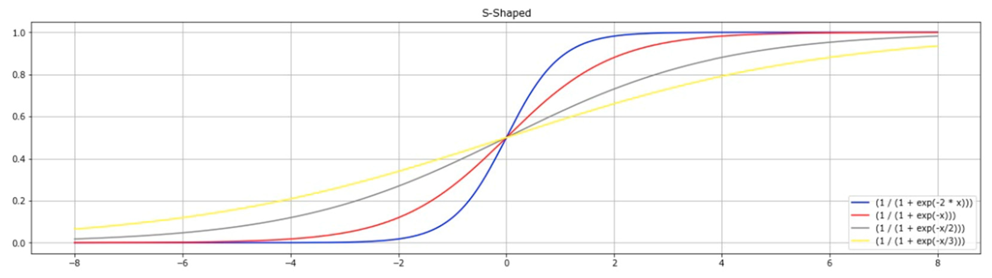
4.1. S-Shaped Transfer Function (S-TF)

This sub will explain the implementation of an S-shaped transfer function. The search agent will move around the binary search space following the S-shaped transfer function [48]. There are four types of S-shaped transfer functions. Figure 4 illustrates the shape of an S-shaped transfer function. The following is an S-shaped transfer function (S1–S4 shaped transfer function) [45] with the following mathematical formula:

$$S1=\frac{1}{1+e^{-2x}}$$

(6)

$$S2=\frac{1}{1+e^{-x}}$$

(7)

$$S3=\frac{1}{1+e^{-\frac{x}{2}}}$$

(8)

$$S4=\frac{1}{1+e^{-\frac{x}{3}}}$$

(9)

The transfer function changes the search from a continuous space to a discrete space following the previous concept [52]. Based on the selected S1–S4 shaped transfer function, the agent positions in the SSA are possibly given as follows [33]:

$$x_i^j\left(t+1\right)=\{\begin{array}{c}0, if random<Sfunction\left(x_i^j\left(t+1\right)\right) \\ 1, if random\ge Sfunction\left(x_i^j\left(t+1\right)\right)\end{array}$$

(10)

A random number drawn from the distribution $\in$[0, 1] where $x_i^j\left(t+1\right),$which is the $i$th element in the solution $x$ in the $j$th dimension.

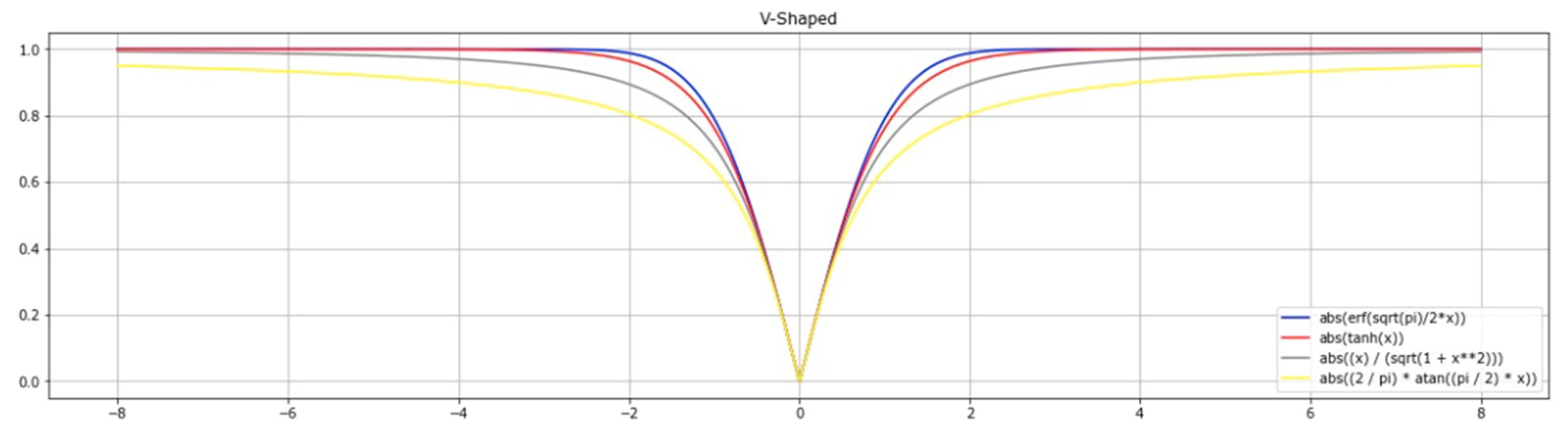
4.2. V-Shaped Transfer Function (V-TF)

Implementation of the V-shaped transfer function will be described in this sub. There are four types of V-shaped transfer functions. Figure 5 illustrates the shape of a V-shaped transfer function. The following is a V-shaped transfer function (V1–V4 shaped transfer function) [45] with the following mathematical formula:

$$V1=\left|\mathit{tanh}\left(x\right)\right|$$

(11)

$$V2=\left|erf\left(\frac{\sqrt{\pi }}{2}x\right)\right|=|\frac{\sqrt{2}}{\pi }{{\displaystyle \int }}_0^{\frac{\sqrt{\pi }}{2}x}{e}^{-t^2}dt|$$

(12)

$$V3=\left|\frac{x}{\sqrt{1+x^2}}\right|$$

(13)

$$V4=\left|\frac{2}{\pi }\mathit{arctan}\frac{\pi }{2} x\right|$$

(14)

Based on the selected V1–V4 shaped transfer function, the agent positions in the SSA are possibly given as follows [36].

$$x_i^j\left(t+1\right)=\{\begin{array}{c}{x}_i^j\left(t\right), if random<Vfunction\left(x_i^j\left(t+1\right)\right) \\ ~x_i^j\left(t\right), if random\ge Vfunction\left(x_i^j\left(t+1\right)\right)\end{array}$$

(15)

A random number is drawn from the distribution $\in$ [0, 1] where $x_i^j\left(t+1\right) ,$which is the $i$th element in the solution $x$ in the $j$th dimension in the $\left(t+1\right)$th iteration. The $j$th dimension of the $i$th solution in the $t$th iterations is represented by $x_i^j\left(t\right)$. $x_i^j\left(t\right)$ is represented by $~x_i^j\left(t\right),$its complement. An $x_i^j\left(t\right)$ value of 0 implies an $~x_i^j\left(t\right)$ value of 1 and vice versa.

4.3. X-Shaped Transfer Function (X1–X2)

In this sub-chapter, the X-shaped transfer function will be presented. There are two types in the X-shaped transfer function family. Figure 6 is an illustration of the X-shaped transfer function. Following are the mathematical formulas of the two types of X-shaped transfer functions [36]:

$$X1=\frac{1}{1+e^x}$$

(16)

$$X2=\frac{1}{1+e^{-x}}$$

(17)

Based on the selected X1–X2 shaped transfer function, the agent positions in the SSA are possibly given as follows [36]:

$$x_i^j\left(t+1\right)=\{\begin{array}{c}1, if random<Xfunction\left(x_i^j\left(t+1\right)\right) \\ 0, if random\ge Xfunction\left(x_i^j\left(t+1\right)\right)\end{array}$$

(18)

$x$_i represent the binary version of Follower i, generated by Equations (16) and (17), respectively, and random $\in$ [0, 1] represents random numbers.

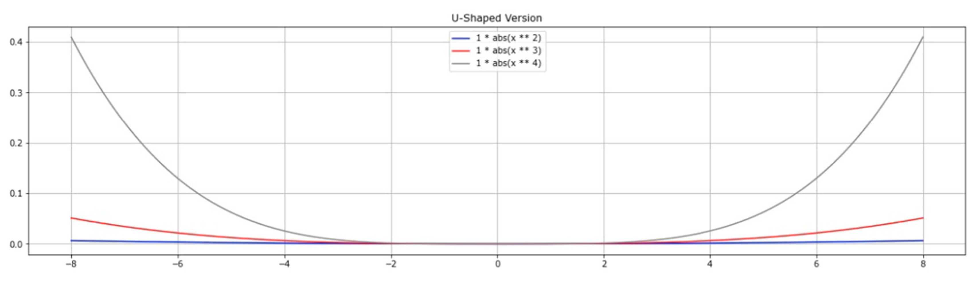
4.4. U-Shaped Transfer Function (U-TF)

BPSO′s U-TF performance was selected to study its impact on BSSA′s discrete feature space performance [37]. The U-TF has been designed with control parameters and can be changed between α and β. The parameters α and β determine the slope and width of the U-TF basin, respectively. There are three types in the U-shaped transfer function family. Figure 7 is an illustration of the U-shaped transfer function. Following are the mathematical formulas of the three types of U-shaped transfer function [37].

$$U1=\alpha \left|x^{\beta }\right|, \alpha =1, \beta =2$$

(19)

$$U2=\alpha \left|x^{\beta }\right|, \alpha =1, \beta =3$$

(20)

$$U3=\alpha \left|x^{\beta }\right|, \alpha =1, \beta =4$$

(21)

Based on the selected U1–U2 shaped transfer function, agent positions in the SSA are possibly given as follows [36]:

$$x_i^j\left(t+1\right)=\{\begin{array}{c}{x}_i^j\left(t\right), if random<Ufunction\left(x_i^j\left(t+1\right)\right) \\ ~x_i^j\left(t\right), if random\ge Ufunction\left(x_i^j\left(t+1\right)\right)\end{array}$$

(22)

In the same way as type V, $x_i^j\left(t\right)$ is represented by $~x_i^j\left(t\right),$its complement. An $x_i^j\left(t\right)$ value of 0 implies an $~x_i^j\left(t\right)$ value of 1 and vice versa. The same as with other types, a random number is drawn from the distribution ∈ [0, 1].

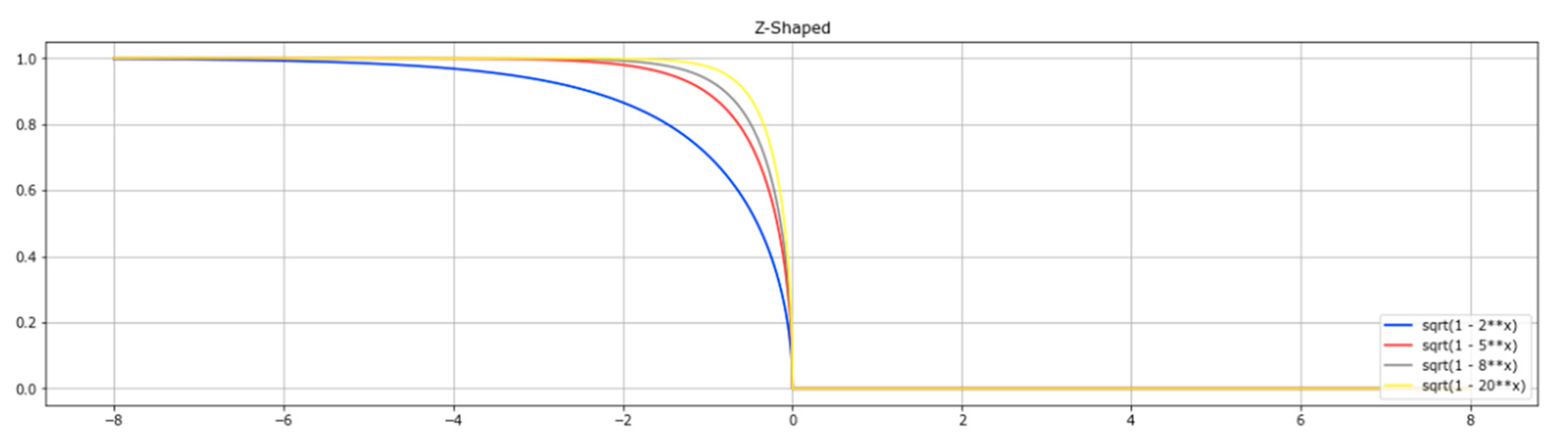
4.5. Z-Shaped Transfer Function (Z-TF)

Z-TF is proposed to optimize the BPSO algorithm [53]. There are four proposed BSSA versions to map a continuous SSA into a binary SSA to solve FS problems. Figure 8 is an illustration of the Z-shaped transfer function. Following are the mathematical formulas of the three types of Z-shaped transfer function [38,39].

$$Z1=\sqrt{1-2^x}$$

(23)

$$Z2=\sqrt{1-5^x}$$

(24)

$$Z3=\sqrt{1-8^x}$$

(25)

$$Z4=\sqrt{1-{20}^x}$$

(26)

Based on the selected Z1–Z4 shaped transfer function, the agent positions in the SSA are possibly given as follows [53]:

$$x_i^j\left(t+1\right)=\{\begin{array}{c}{x}_i^j\left(t\right), if random<Zfunction\left(x_i^j\left(t+1\right)\right) \\ ~x_i^j\left(t\right), if random\ge Zfunction\left(x_i^j\left(t+1\right)\right)\end{array}$$

(27)

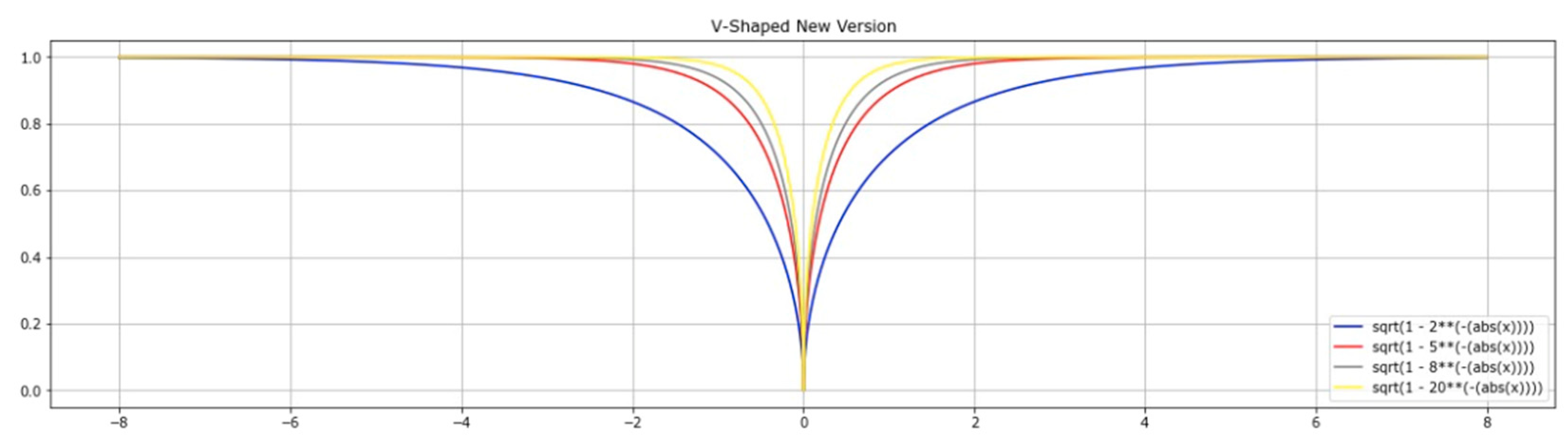
4.6. New Version V-Shaped Transfer Function (New Version V-TF)

In this study, we propose a new version of the V-shaped transfer function. The new version V-shaped transfer function type is the same as the previous original V-shaped transfer function type, which has four types of the V-shaped transfer function family, but the difference is that the new version V-shaped transfer function offers a math formula that is simpler than the original type of V-shaped transfer function family. However, the new version V-shaped transfer function is also able to control the agent to move around the binary 0 and 1 search space following the new version V-shaped transfer function illustrated in Figure 9.

Following are the mathematical formulas of the four types of new version V-shaped transfer functions proposed:

$$New V1=\sqrt{1-2^{-\left|x\right|}}$$

(28)

$$New V2=\sqrt{1-5^{-\left|x\right|}}$$

(29)

$$New V3=\sqrt{1-8^{-\left|x\right|}}$$

(30)

$$New V4=\sqrt{1-{20}^{-\left|x\right|}}$$

(31)

Based on the selected new version V1–V4 shaped transfer function, the agent positions in the SSA are possibly given as follows:

$$x_i^j\left(t+1\right)=\{\begin{array}{c}{x}_i^j\left(t\right), if random<New V function\left(x_i^j\left(t+1\right)\right) \\ ~x_i^j\left(t\right), if random\ge New V function\left(x_i^j\left(t+1\right)\right)\end{array}$$

(32)

In the same way as type V, $x_i^j\left(t\right)$ is represented by $~x_i^j\left(t\right),$its complement. An $x_i^j\left(t\right)$ value of 0 implies an $~x_i^j\left(t\right)$ value of 1 and vice versa. The same as with other types, a random number is drawn from the distribution ∈ [0, 1]. The proposed pseudocode for an improved SSA and transfer function is shown in Algorithm 2:

Algorithm 2. Salp Swarm Algorithm-Transfer Function (SSA-TF)

Input parameter: Population Size, Number of Iterations, Min Values, Max Values, α dan β for U-TF

(1) Initialize the salp population $x_i$ ($i=1, 2, 3, \dots , n)$considering ub and lb

(2) initialize the TF type (S-TF using Equations (6)–(9) or the V-TF using Equations (11)–(14) or the X-TF using Equations (16) and (17) or the U-TF using Equations (19)–(21) or the Z-TF using Equations (23)–(26) or the new version V-TF using Equations (28)–(31)

(3) while (end condition is not satisfied) do

(4) calculate the fitness of each search agent (salp)

(5) $F=$ the best search agent

(6) update $c_1$ by Equation (3)

(7)  for each salp ($x_i$)

(8)    if $\left(i==1\right)$

(9)       based on the probability value of the TF, the SSA will determine the sampling that has the highest information based on Equation (10) for the S-TF type, or Equation (15) for the V-TF type, or Equation (18) for the X-TF type, or Equation (22) for the U-TF type, or Equation (27) for the Z-TF type, or Equation (32) for the V-TF new version type

(10)       update the position of the leading salp using Equation (2)

(11)    else (12)       update the position of the follower salp using Equation (5) (13)    end (14)  end

(15) amend the salps based on the upper and lower bounds of variables

(16) end

(17) return F

Output: Global best solution

The SSA-TF algorithm has the same complexity as the SSA. The transfer function used to modify the SSA does not affect the complexity of the SSA-TF. Where if seen from the pseudocode of the SSA-TF algorithm, after initialization, the population of the salp, then initializing as the type of TF to be used. Based on the TF probability value, the SSA will determine the sampling with the highest information based on the equation that allows the agent position in the SSA algorithm to update the salp leader position. This has absolutely no effect on the complexity of the SSA-TF.

Making use of the transfer function (TF) is an effective way to convert continuous optimizations to the binary version. The TF is a mathematical function that determines the probability of changing a position vector dimension from 0 to 1 and vice versa [51]. But what is no less important is that the TF is an operator that is very easy to implement, with its ability to increase the SSA exploitation and exploration in feature selection [38].

5. Application of Salp Swarm Algorithm (SSA) Using Transfer Function (SSA-TF) for Feature Selection in Sentiment Analysis

In the case of large datasets, including the sentiment analysis domain, a practical approach with low computational costs is needed, namely using feature selection techniques. Assuming that the dataset has M features, 2^M feature subsets will be selected [39]. The feature selection technique with a metaheuristic approach overcomes the problem of generating all possible combinations of features that are calculated [36,43]. The metaheuristic approach to optimization algorithms has attracted the attention of researchers because of its advantages, such as simplicity, few parameters, derivation-free mechanism and avoidance of local optimization [41]. Optimization algorithms have advantages over the normal search, including choosing optimal or close-to-optimal subsets of features in an acceptable amount of time [17]. All solutions for FS are binary because they are discrete problems [30]. The optimizer′s binarization process heavily relies on the transfer function. They identify the possibility of updating the positional solution by changing its characteristics from 0 to 1 and vice versa [51]. A binary SSA, i.e., the SSA, uses the TF to explore and exploit to find the ideal feature subset in the feature search space (fitness). Feature subsets are evaluated by optimizing two conflicting objectives simultaneously with a fitness function. The objective is the classification algorithm′s performance and the dataset′s number of features. The classification algorithms used in this study to evaluate the selected feature subsets include k-nearest neighbor (KNN), support vector machine (SVM) and naïve Bayes.

Binary vectors are used to model a feature subset in this paper. There are as many features in the problem as in this vector. A feature is assigned a value of 1 when selected; otherwise, it is assigned a value of 0. Two criteria determine a feature subset′s excellence: the minimum inaccuracy rate (maximum classification accuracy) and the minimum number of features selected. A fitness function combines these opposing objectives. The fitness function equation is shown as follows [54]:

$$Fitness=\alpha {\gamma }_R\left(D\right)+\beta \frac{\left|R\right|}{\left|C\right|}$$

(33)

Based on Equation (33), the classifier misclassification value is indicated by γ_R (D). The number of features selected in the reduction is indicated by |R|. The number of conditional features in the dataset is indicated by |C|. Factors to show superior quality and subset length based on observations and recommendations are shown by α ∈[1, 0],β = (1 − α) [48]. The fitness results are shown in Appendix B in Figure A1.

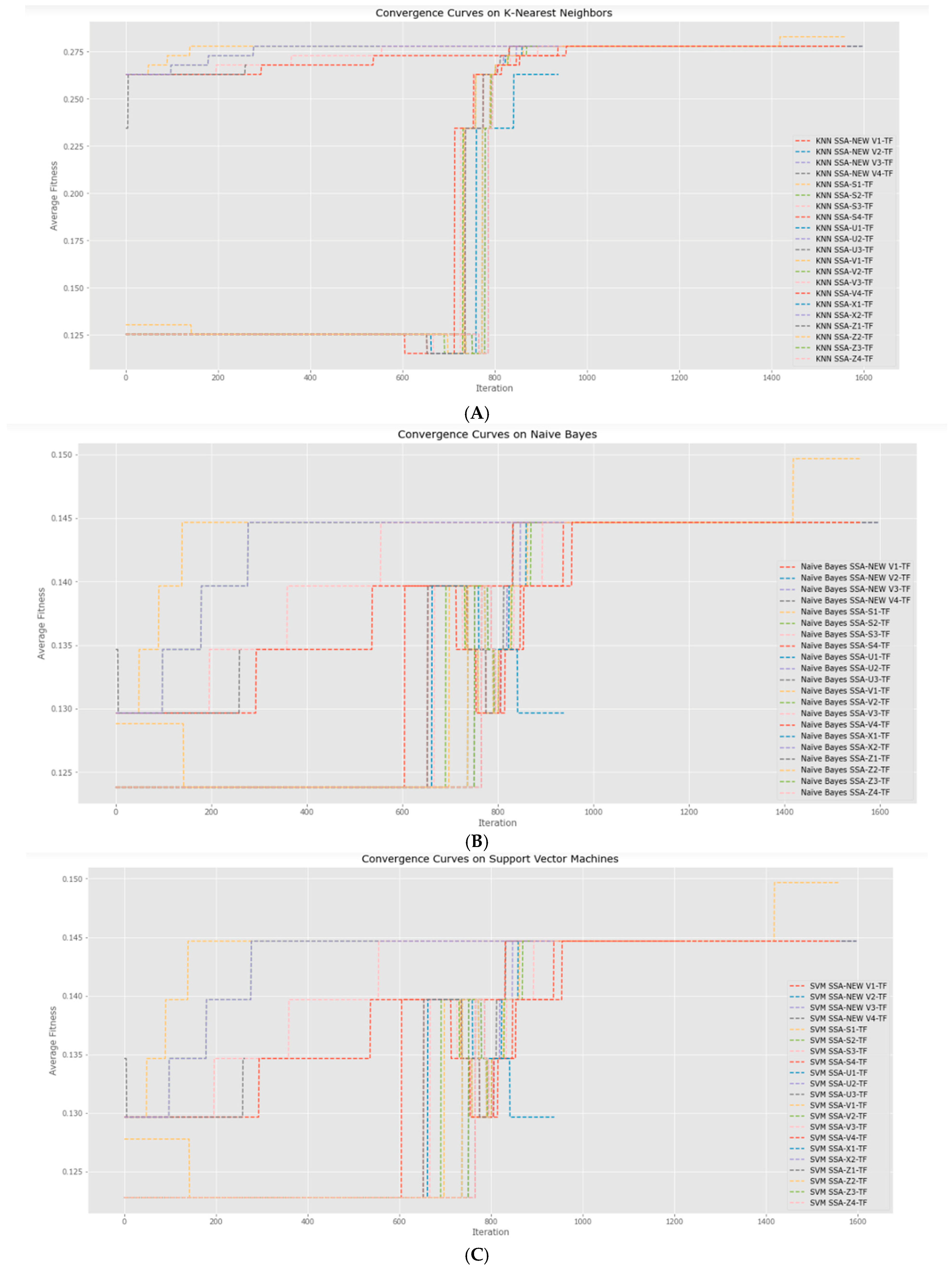
6. Experimental Results of This Study

In this section, we summarize the results of the SSA using a transfer function (SSA-TF) and its implementation for feature selection in sentiment analysis.

6.1. Dataset Benchmark

To evaluate the efficiency of the proposed algorithm, the dataset benchmark used was public data taken from Kaggle, called Twitter US Airline Sentiment [44]. There are 14,601 records in this dataset. These data contain public opinions about the service of six airlines in the United States in order to firstly classify tweets as positive, negative and neutral, followed by categorizing negative reasons (such as “flight late” or “deficient service”). A tweet′s positivity, negativity or neutrality was determined by the Twitter user′s feedback about the airline. These data were selected because they cover a wide variety of characteristics with different features and instances.

6.2. Experiment Setup

This section will investigate the performance of the salp swarm algorithm transfer function (SSA-TF). Using the US Airlines Twitter benchmark dataset from Kaggle, this algorithm was used as a feature selection. Then, selected feature subsets were evaluated using classification algorithms such as k-nearest neighbor, support vector machine and naive Bayes. K-nearest neighbor, support vector machine and naive Bayes were chosen because the three classification algorithms are popular and their performance is excellent in classification in sentiment analysis [55]. The k-nearest neighbor (KNN) algorithm with the Euclidean distance metric and $k$ = 25 was used. This is because, based on previous experiments, this value produces high accuracy and faster time performance. Three types of algorithms were used in the naive Bayes algorithm, including Bernoulli, Gaussian and multinomial. Then linear, polynomial and RBF were the three types used in the support vector machine algorithm. In this paper, our dataset was divided into K-folds. We used a persisting strategy where each dataset was partitioned into ten-fold. Python 3.9.7, Jupyter Notebook, Google Collabs Pro+, a system with an Intel i7 3.30 Hz CPU, a 1 TB SSD and 16 GB of RAM were used to calculate all of the results under the same conditions.

The SSA-TF was also compared with other conventional optimization algorithms, such as particle swarm optimization (PSO) and ant lion optimization (ALO), to measure its performance based on its accuracy, precision, recall, F-1 and time complexity.

Table 1. Parameter settings.

Parameter	Value
$k$ in k-nearest neighbor	25
Bernoulli, Gaussian and multinomial type in naïve Bayes	Bernoulli
Linear, polynomial and RBF type in support vector machine	Linear
C in support vector machine	1
Population size in SSA	10
Number of iterations in SSA	10
Min. values in SSA	5
Max. values in SSA	50
Population size in PSO	250
Number of iterations in PSO	10
Min. values in PSO	5
Max. values in PSO	50
$\omega$ (inertia weight) in PSO	0.9
$c1 and c2$ in PSO	2
Exponential decay weight in PSO	0
Verbosity level of the screen output in PSO	True
Number of iterations in ALO	10
Min. values in ALO	5
Max. values in ALO	50
Dimension	Number of features
$k$ in K-fold cross validation	10
Transfer function	(−8, 8) with different per step 0.01
Max df in TfidfVectorizer	0.7
Min df in TfidfVectorizer	0.1
Max features in TfidfVectorizer	100
N-gram range in TfidfVectorizer	(1, 2)
Stopwords in TfidfVectorizer	English

lists the specific parameters set for the optimization algorithm and the classifier algorithm used.

6.3. Comparison Algorithms and Evaluation Metrics

A comparison of four algorithms (SSA, PSO, ALO and SSA-TF) and 21 variants of the SSA-TF algorithm was investigated. The results show that the modified SSA-TF variant (SSA-new V-TF) outperformed the other three algorithms (SSA, PSO and ALO) and 20 SSA-TF variants in all tests using the naive Bayes, KNN and SVM classifier algorithms. Metrics such as accuracy, precision, recall, F-1, processing time and feature probability were measured in this study. The results of obtaining accuracy, precision, recall, F-1, processing time performance and feature probability values for all SSA-TF algorithms and variants are recorded in

Table A1. Comparison accuracy, precision, recall, F-1, time processing and feature probability of various SSA-TF versions and other conventional optimizers with classifier machine learning.

Algorithm	TF-Family	Accuracy	Precision	Recall	F-1	Time Processing (ns)	Feature Probability
Naive Bayes SSA-S1-TF	S-TF	0.760679362	0.830447267	0.757222325	0.745670964	0.012069225	5
Naive Bayes SSA-S2-TF	S-TF	0.760679362	0.830447267	0.757222325	0.745670964	0.012586117	5
Naive Bayes SSA-S3-TF	S-TF	0.760679362	0.830447267	0.757222325	0.745670964	0.012335062	5
Naive Bayes SSA-S4-TF	S-TF	0.760679362	0.830447267	0.757222325	0.745670964	0.018228531	5
KNN SSA-S1-TF	S-TF	0.494081318	0.603785419	0.501490565	0.335142402	0.517837763	5
KNN SSA-S2-TF	S-TF	0.494081318	0.603785419	0.501490565	0.335142402	0.623624563	5
KNN SSA-S3-TF	S-TF	0.494081318	0.603785419	0.501490565	0.335142402	0.550310850	5
KNN SSA-S4-TF	S-TF	0.494081318	0.603785419	0.501490565	0.335142402	0.436069489	5
SVM SSA-S1-TF	S-TF	0.760679362	0.830447267	0.757222325	0.745670964	0.310822964	5
SVM SSA-S2-TF	S-TF	0.760679362	0.830447267	0.757222325	0.745670964	0.200889826	5
SVM SSA-S3-TF	S-TF	0.760679362	0.830447267	0.757222325	0.745670964	0.249196768	5
SVM SSA-S4-TF	S-TF	0.760679362	0.830447267	0.757222325	0.745670964	0.303336382	5
Naive Bayes SSA-V1-TF	V-TF	0.802367473	0.830447267	0.803337636	0.801810532	0.010612965	6
Naive Bayes SSA-V2-TF	V-TF	0.802367473	0.830447267	0.803337636	0.801810532	0.038087845	5
Naive Bayes SSA-V3-TF	V-TF	0.802367473	0.830447267	0.803337636	0.801810532	0.010998964	5
Naive Bayes SSA-V4-TF	V-TF	0.802367473	0.830447267	0.803337636	0.801810532	0.014706612	5
KNN SSA-V1-TF	V-TF	0.809572826	0.840406878	0.807548098	0.805325383	0.523573875	6
KNN SSA-V2-TF	V-TF	0.809572826	0.840406878	0.807548098	0.805325383	0.603285313	5
KNN SSA-V3-TF	V-TF	0.809572826	0.840406878	0.807548098	0.805325383	0.473382950	5
KNN SSA-V4-TF	V-TF	0.809572826	0.840406878	0.807548098	0.805325383	0.487081051	5
SVM SSA-V1-TF	V-TF	0.809572826	0.840406878	0.807548098	0.805325383	0.563572645	6
SVM SSA-V2-TF	V-TF	0.809572826	0.840406878	0.807548098	0.805325383	0.399179459	5
SVM SSA-V3-TF	V-TF	0.809572826	0.840406878	0.807548098	0.805325383	0.642655611	5
SVM SSA-V4-TF	V-TF	0.809572826	0.840406878	0.807548098	0.805325383	0.621925592	5
Naive Bayes SSA-X1-TF	X-TF	0.802367473	0.830447267	0.803337636	0.801810532	0.007063866	5
Naive Bayes SSA-X2-TF	X-TF	0.760679362	0.830447267	0.757222325	0.745670964	0.007018566	5
KNN SSA-X1-TF	X-TF	0.809572826	0.840406878	0.807548098	0.805325383	0.476012707	5
KNN SSA-X2-TF	X-TF	0.494081318	0.603785419	0.501490565	0.335142402	0.406121969	5
SVM SSA-X1-TF	X-TF	0.804426145	0.830447267	0.803014936	0.802180902	0.522874117	5
SVM SSA-X2-TF	X-TF	0.760679362	0.830447267	0.757222325	0.745670964	0.243289471	5
Naive Bayes SSA-U1-TF	U-TF	0	0	0	0	0	0
Naive Bayes SSA-U2-TF	U-TF	0	0	0	0	0	0
Naive Bayes SSA-U3-TF	U-TF	0.760679362	0.830447267	0.757222325	0.745670964	0.005551100	3
KNN SSA-U1-TF	U-TF	0	0	0	0	0	0
KNN SSA-U2-TF	U-TF	0	0	0	0	0	0
KNN SSA-U3-TF	U-TF	0.560988163	0.646807540	0.566522220	0.494644980	0.192241669	3
SVM SSA-U1-TF	U-TF	0	0	0	0	0	0
SVM SSA-U2-TF	U-TF	0	0	0	0	0	0
SVM SSA-U3-TF	U-TF	0.760679362	0.830447267	0.757222325	0.745670964	0.118218000	3
Naive Bayes SSA-Z1-TF	Z-TF	0.802367473	0.830447267	0.803337636	0.801810532	0.011059284	5
Naive Bayes SSA-Z2-TF	Z-TF	0.802367473	0.830447267	0.803337636	0.801810532	0.012661219	5
Naive Bayes SSA-Z3-TF	Z-TF	0.802367473	0.830447267	0.803337636	0.801810532	0.012352228	5
Naive Bayes SSA-Z4-TF	Z-TF	0.802367473	0.830447267	0.803337636	0.801810532	0.016859770	5
KNN SSA-Z1-TF	Z-TF	0.809572826	0.840406878	0.807548098	0.805325383	0.482684851	5
KNN SSA-Z2-TF	Z-TF	0.809572826	0.840406878	0.807548098	0.805325383	0.488482714	5
KNN SSA-Z3-TF	Z-TF	0.809572826	0.840406878	0.807548098	0.805325383	0.436493635	5
KNN SSA-Z4-TF	Z-TF	0.809572826	0.840406878	0.807548098	0.805325383	0.623229980	5
SVM SSA-Z1-TF	Z-TF	0.804426145	0.830447267	0.803014936	0.802180902	0.410887957	5
SVM SSA-Z2-TF	Z-TF	0.804426145	0.830447267	0.803014936	0.802180902	0.414152384	5
SVM SSA-Z3-TF	Z-TF	0.804426145	0.830447267	0.803014936	0.802180902	0.493735790	5
SVM SSA-Z4-TF	Z-TF	0.804426145	0.830447267	0.803014936	0.802180902	0.438720942	5
Naive Bayes SSA-New V1-TF	New V-TF	0.802367473	0.830447267	0.803337636	0.801810532	0.010612965	6
Naive Bayes SSA-New V2-TF	New V-TF	0.802367473	0.830447267	0.803337636	0.801810532	0.038087845	5
Naive Bayes SSA-New V3-TF	New V-TF	0.802367473	0.830447267	0.803337636	0.801810532	0.010998964	5
Naive Bayes SSA-New V4-TF	New V-TF	0.802367473	0.830447267	0.803337636	0.801810532	0.014706612	5
KNN SSA-New V1-TF	New V-TF	0.809572826	0.840406878	0.807548098	0.805325383	0.603285313	5
KNN SSA-New V2-TF	New V-TF	0.809572826	0.840406878	0.807548098	0.805325383	0.473382950	5
KNN SSA-New V3-TF	New V-TF	0.809572826	0.840406878	0.807548098	0.805325383	0.388332605	5
KNN SSA-New V4-TF	New V-TF	0.809572826	0.840406878	0.807548098	0.805325383	0.893996000	5
SVM SSA-New V1-TF	New V-TF	0.804426145	0.830447267	0.803014936	0.802180902	0.399179459	5
SVM SSA-New V2-TF	New V-TF	0.804426145	0.830447267	0.803014936	0.802180902	0.642655611	5
SVM SSA-New V3-TF	New V-TF	0.804426145	0.830447267	0.803014936	0.802180902	0.621925592	5
SVM SSA-New V4-TF	New V-TF	0.804426145	0.830447267	0.803014936	0.802180902	0.695250034	5
Naive Bayes SSA	-	0.59	0.196667	0.333333	0.244522	1,455,331,000	5
KNN SSA	-	0.55	0.343373	0.42504	0.366227	1,879,957,000	5
SVM SSA	-	0.6	0.232963	0.366667	0.279599	1,336,488,000	5
Naive Bayes PSO	-	0.760679	0.830447	0.757222	0.745671	4,576,292,000	5
KNN PSO	-	0.809573	0.807548	0.840407	0.805325	2,187,501,000	5
SVM PSO	-	0.804426	0.830447	0.803015	0.802181	5,704,434,000	5
Naive Bayes ALO	-	0.802367	0.810447	0.807548	0.805325	1,462,639,000	5
KNN ALO	-	0.804426	0.790432	0.803015	0.802181	2,108,248,000	5
SVM ALO	-	0.809573	0.820741	0.801811	0.803338	1,229,433,000	5
Naive Bayes	-	0.57	0.200741	0.333333333	0.247703	1,283,777,000	5
KNN	-	0.57	0.195	0.325	0.239893	1,330,194,000	5
SVM	-	0.6	0.232963	0.366667	0.279599	1,141,390,000	5

. Furthermore, Table A1 shows that the rate of the SSA-new V3-TF was faster and obtained the highest accuracy value than the other three algorithms and other variants for the benchmark dataset tested. Based on the observation results, it can be concluded that the proposed SSA-new V3-TF has better quality and stability than the others.

Based on Table A1, it can be seen that there are 19 algorithms that recorded the highest accuracy with an accuracy value of 80.96%, which is obtained by KNN SSA-V1-V4-TF, SVM SSA-V1-V4-TF, KNN SSA-X1-TF, KNN SSA-Z1-Z4-TF, KNN SSA-new V1-V4-TF, KNN PSO and SVM ALO. There is something interesting about obtaining the highest accuracy for all of them obtained with the KNN classifier. For all new types of V-shaped transfer functions (new V1-V4 TF), the highest accuracy value was obtained using the KNN algorithm. Likewise, all types of Z1-Z4-TF, X1-TF and V1-V4-TF obtained the highest accuracy value using the KNN classifier algorithm. In addition to the KNN algorithm, SSA-V1-V4-TF also achieved the highest accuracy, of 80.96%, using the SVM algorithm. Likewise, SVM ALO managed to obtain the same accuracy.

Other optimization algorithms were used as a comparison besides the SSA-TF, such as the SSA, PSO and ALO. Only PSO and ALO were able to align with optimal performance with the SSA-TF algorithm. The SSA tested for all tested classifiers obtained very low accuracy, which was around 55.00–60.00%. This was similar to using a classifier without an optimization algorithm for feature selection that only uses the KNN, naive Bayes and SVM classifiers, the three of which also produced a very low accuracy of 57.00–60.00%, as well as precision, recall and F-1 results with an average yield that was almost below 40.00%. We expected this to occur because the preprocessing used did not use CountVect, so it directly used TF-IDF as word weight. The challenge was that when using CountVect and TF-IDF, there were many point vectors which were a problem for conventional optimization algorithms to apply for feature selection techniques in sentiment analysis. This was because, based on the results of the accuracy values obtained, there were still 13 algorithms that occupy the same rank. We tried to analyze the next metric based on the processing time and the possible features selected in addition to the low accuracy, precision, recall and F-1 metrics. Other metrics, such as processing time, also obtained long results.

The advantage of the SSA-TF algorithm compared to other metaheuristic algorithms was its processing time. Most of the metaheuristic-based optimization algorithms for FST in SA were weak when faced with high-dimensional data with many features. Thus, making the processing time long like other optimization algorithms that were compared in this study for feature selection in SA, namely the SSA, PSO and ALO. The interesting fact was that, for the English dataset used, PSO and ALO were able to perform optimally for feature selection. KNN-PSO was able to perform optimally as a feature selection in SA with an accuracy value of up to 80.96%, as well as SVM-ALO. Only the processing time metrics obtained were very long, namely 2,187,501,000 nanoseconds (ns) or the equivalent of 2.5 days for the KNN-PSO algorithm and 1,229,433,000 nanoseconds (ns) or the equivalent of 1.4 days for the SVM-ALO algorithm. The conventional SSA optimization [32], where the initial study of each salp moved in the search space to a position of continuous value. However, in the case of feature selection on text data, the search space was modelled as an n-dimensional Boolean grid, where the salp moved across the corners of the hypercube. Since the problem was to select or deselect a given feature, the salp position was represented by a binary vector. So, we needed a binary version of the salp swarm algorithm, which limited new salp positions to only binary values using the transfer function. Although, based on accuracy metrics on the KNN SSA-S-TF algorithm, it was superior to research algorithm that was applied as a feature selection to the KNN, SVM and naive Bayes classifier algorithms only obtained accuracy values in the range of 55.00%–60.00%. This was in accordance with the existing literature in [32] which reaches 80.80%, it was still inferior to PSO for time processing. So, in our research, we tried to offer the SSA algorithm using a new version of the transfer function of type V.

Based on Table A1 and referring to the previous highest accuracy value, KNN and SSA with the new V3-shaped transfer function had better performance for feature selection algorithms in sentiment analysis. New V3-TF is a transfer function that plays a perfect role in controlling the SSA optimization algorithm. When combined, it was very suitable and performed better with a fastest processing time of only 0.39 nanoseconds (ns).

With the dissemination of this research, it is hoped that readers will know that an SSA-new V-TF algorithm can be used as an optimization algorithm for feature selection in sentiment analysis with optimal performance and a fast processing time. Furthermore, this study is part of our big work to build an optimization model as a feature selection in the sentiment analysis case of forest and land fires that occurred in Indonesia and was a trending topic in 2019 on Twitter. This is our next research plan.

6.4. Statistical Test to Support the Evaluation Metrics Results Obtained

By using the R studio programming language, statistical tests were carried out. Statistical testing was carried out aiming to determine whether there was sufficient evidence to reject or accept the hypothesis. There were many statistical tests, including the z-test, t-test, Mann Withney, Kruskal Wallis, Anova and Ancova. In this study, the results of statistical testing of the t-test type based on accuracy and time processing metrics were carried out using the R studio programming language.

Based on

Table 2. The results of statistical testing of the t-test type based on the accuracy metric of the SSA-new V-TF algorithm as the best optimization algorithm with SSA-S-TF, SSA-V-TF, SSA-X-TF, SSA-U-TF and SSA-Z-TF algorithm.

t-Statistic	p-Value	Compared Algorithm
$3.4469$	0.9973	SSA-S-TF
−2.3452	0.01941	SSA-V-TF
1.3242	0.8786	SSA-X-TF
4.1287	0.9955	SSA-U-TF
NA	NA	SSA-Z-TF

, the t-statistic is the value of t, which was influenced by the mean, number of samples and standard deviation of the data. The p-value was the likelihood of the null hypothesis measured by the p-value, which was the probability that took a value between 0 and 1. The p-value was directly proportional to the probability of the null hypothesis, so the smaller the p-value, the more implausible the null hypothesis.

Based on the rules of statistical testing with the t-test type, the hypothesis was accepted if the p-value > α. The α value was 0.05. Table 2 shows that the p-value greater than the α value of 0.05 was the SSA new V-TF algorithm compared to the SSA-S-TF, SSA-X-TF and SSA-U-TF algorithms. Therefore, it can be said that the hypothesis of the SSA new V-TF algorithm was superior to optimal performance based on the accuracy metrics of the SSA-S-TF, SSA-X-TF and SSA-U-TF algorithms, which are acceptable. The rest of the SSA-V-TF and SSA-Z-TF algorithms, the SSA new V-TF hypothesis were superior but cannot be accepted because the p-value < α value. This shows that the accuracy metrics on the SSA new V-TF algorithm were not superior to the SSA V-TF and SSA-Z-TF algorithms based on Table 2. These three algorithms had accuracy values above 80.00% for all types of TF. In addition to accuracy metrics, this study also conducted statistical tests (t-tests) based on the processing time metrics shown in

Table 3. The results of statistical testing of the t-test type based on the time processing metric of the SSA-new V-TF algorithm as the best optimization algorithm with the SSA-S-TF, SSA-V-TF, SSA-X-TF, SSA-U-TF and SSA-Z-TF algorithm.

t-Statistic	p-Value	Compared Algorithm
$1.9715$	0.9628	SSA-S-TF
0.73696	0.7617	SSA-V-TF
1.1743	0.8534	SSA-X-TF
3.6943	0.997	SSA-U-TF
2.3491	0.9807	SSA-Z-TF

.

The overall results of the p-value in Table 3 show that the p-value > α (0.05). Therefore, this shows that the hypothesis was accepted that the SSA-new V-TF algorithm was superior to the SSA-S-TF, SSA-V-TF, SSA-X-TF, SSA-U-TF and SSA-Z-TF algorithms based on processing time metrics. Table A1 is the result of a comparison of accuracy, precision, recall, F-1, processing time and feature probability of various versions of the SSA-TF and other conventional optimizers with classifier machine learning. In this section, the visualization of Table A1 is also displayed graphically in Figure A2.

7. Conclusions

In order to solve the FS problem, an improved binary SSA-based optimizer with a transfer function is proposed in this paper. The proposed method, which includes 21 transfer function types from six TF shape families (S-shaped transfer function, V-shaped transfer function, X-shaped transfer function, U-shaped transfer function, Z-shaped transfer function and a new version of the V-shaped transfer function), was tested on a single set of benchmark data that is regarded as being of high quality. Classification accuracy, precision, recall, F-1 and processing time were studied and statistical tests were also provided in detail in order to find the best TF for the binary version. The SSA with TF in the form of the new version of the V-shaped transfer function type (SSA-new V3-TF) for the KNN algorithm performed better than the other proposed versions, as can be seen from a comparison between all of them. The results obtained from the SSA-new V3-TF algorithm as a feature selection in the KNN algorithm obtained the best accuracy values, reaching 80.96%, precision, recall and F-1 obtained, respectively, 84.04%, 80.75% and 80.53%. In addition, the KNN SSA new V3-TF algorithm obtained the best model processing time, which was only 0.388 nanoseconds (ns). This was better than using only the KNN-SSA algorithm without modifying the transfer function, which only obtained an accuracy of 55.00% and the processing time was quite long, namely 1,879,957,000 nanoseconds (ns), which is equivalent to 2.18 days. There was an exciting fact: another type of transfer function family in the form of the new version V-TF produced the same accuracy, reaching 80.96% for the KNN algorithm, but the processing time was longer, reaching 0.473 nanoseconds (ns) for KNN SSA-new V2-TF, 0.603 nanoseconds (ns) for KNN SSA-new V1-TF and 0.894 nanoseconds (ns) for KNN SSA-new V4-TF.

Apart from the KNN SSA-new V1-V4-TF algorithm, several other algorithms had the highest accuracy value, reaching 80.96%, such as KNN-SSA V1-V4-TF, KNN SSA-X1-TF, KNN SSA-Z1-Z4-TF, SVM SSA V1-V4-TF, KNN PSO and SVM ALO. Even though they both had the best accuracy, precision, recall and F-1, in terms of processing time metrics, they were still inferior to KNN SSA-new V3-TF. One of them was KNN PSO, with a processing time of 2,187,501,000 nanoseconds (ns), equivalent to 2.5 days, and SVM ALO, with a processing time of 1,229,433,000 nanoseconds (ns), which is equivalent to 1.4 days. Therefore, the KNN SSA-new V3-TF algorithm performed optimally for use as a feature selection in English sentiment analysis.

Opportunities for future research using the SSA-new V3-TF optimization algorithm are very high. Further research will test various datasets using SSA-new V3-TF for feature selection. Future research will also focus on the performance of SSA-new V3-TFs with Indonesian-language datasets for sentiment analysis and various machine-learning tasks. One of them is opinion data from social media about forest and land fires, which became a trending topic in 2019 on Twitter. Future studies could examine whether the new version of V-TF can also be tested on other optimization algorithms that have problems when faced with dimensions (total features) and data size, such as PSO, GA, ACO and ALO as optimization algorithms for FST in SA. Besides that, in subsequent studies, the impact that new TF families or new variations of existing TF families with simpler mathematical formulas of the form S, X, Z, or U may have on binary SSA or other binary algorithms.

References

1. W. are S. Hootsuite. Digital 2022 Global Overview Report. 26 January 2022. Available online: https://wearesocial.com/sg/blog/2022/01/digital-2022-another-year-of-bumper-growth/ (accessed on 2 February 2020).
2. Arif, M.H.; Li, J.; Iqbal, M.; Liu, K. Sentiment analysis and spam detection in short informal text using learning classifier systems. Soft Comput. 2018, 22, 7281–7291. [Google Scholar] [CrossRef]
3. Hangya, V.; Farkas, R. A comparative empirical study on social media sentiment analysis over various genres and languages. Artif. Intell. Rev. 2017, 47, 485–505. [Google Scholar] [CrossRef]
4. Agarwal, A.; Toshniwal, D. Application of Lexicon Based Approach in Sentiment Analysis for short Tweets. In Proceedings of the 2018 International Conference on Advances in Computing and Communication Engineering, ICACCE 2018, Paris, France, 22–23 June 2018; pp. 189–193. [Google Scholar] [CrossRef]
5. Pandey, A.C.; Rajpoot, D.S. Improving Sentiment Analysis using Hybrid Deep Learning Model. Recent Adv. Comput. Sci. Commun. 2019, 13, 627–640. [Google Scholar] [CrossRef]
6. Binsar, F.; Mauritsius, T. Mining of Social Media on Covid-19 Big Data Infodemic in Indonesia. J. Comput. Sci. 2020, 16, 1598–1609. [Google Scholar] [CrossRef]
7. Wrycza, S.; Maślankowski, J. Social Media Users’ Opinions on Remote Work during the COVID-19 Pandemic. Thematic and Sentiment Analysis. Inf. Syst. Manag. 2020, 37, 288–297. [Google Scholar] [CrossRef]
8. Dhaoui, C.; Webster, C.M.; Tan, L.P. Social media sentiment analysis: Lexicon versus machine learning. J. Consum. Mark. 2017, 34, 480–488. [Google Scholar] [CrossRef]
9. Hartmann, J.; Huppertz, J.; Schamp, C.; Heitmann, M. Comparing automated text classification methods. Int. J. Res. Mark. 2019, 36, 20–38. [Google Scholar] [CrossRef]
10. Ahmad, S.R.; Bakar, A.A.; Yaakub, M.R. A review of feature selection techniques in sentiment analysis. Intell. Data Anal. 2019, 23, 159–189. [Google Scholar] [CrossRef]
11. Deniz, A.; Angin, M.; Angin, P. Evolutionary Multiobjective Feature Selection for Sentiment Analysis. IEEE Access 2021, 9, 142982–142996. [Google Scholar] [CrossRef]
12. Nafis, N.S.M.; Awang, S. An Enhanced Hybrid Feature Selection Technique Using Term Frequency-Inverse Document Frequency and Support Vector Machine-Recursive Feature Elimination for Sentiment Classification. IEEE Access 2021, 9, 52177–52192. [Google Scholar] [CrossRef]
13. Abdi, A.; Shamsuddin, S.M.; Hasan, S.; Piran, J. Machine learning-based multi-documents sentiment-oriented summarization using linguistic treatment. Expert Syst. Appl. 2018, 109, 66–85. [Google Scholar] [CrossRef]
14. Naz, M.; Zafar, K.; Khan, A. Ensemble based classification of sentiments using forest optimization algorithm. Data 2019, 4, 76. [Google Scholar] [CrossRef]
15. Hassonah, M.A.; Al-Sayyed, R.; Rodan, A.; Al-Zoubi, A.M.; Aljarah, I.; Faris, H. An efficient hybrid filter and evolutionary wrapper approach for sentiment analysis of various topics on Twitter. Knowl. -Based Syst. 2020, 192, 105353. [Google Scholar] [CrossRef]
16. Bahassine, S.; Madani, A.; Al-Sarem, M.; Kissi, M. Feature selection using an improved Chi-square for Arabic text classification. J. King Saud Univ. - Comput. Inf. Sci. 2020, 32, 225–231. [Google Scholar] [CrossRef]
17. Tubishat, M.; Ja’Afar, S.; Alswaitti, M.; Mirjalili, S.; Idris, N.; Ismail, M.A.; Omar, M.S. Dynamic Salp swarm algorithm for feature selection. Expert Syst. Appl. 2021, 164, 113873. [Google Scholar] [CrossRef]
18. Yang, X.-S. Engineering Optimization an Introduction with Metaheuristic Applications; John Wiley & Sons, Inc.: Hoboken, NJ, USA, 2010. [Google Scholar]
19. Ahmad, S.R.; Bakar, A.A.; Yaakub, M.R. Ant colony optimization for text feature selection in sentiment analysis. Intell. Data Anal. 2019, 23, 133–158. [Google Scholar] [CrossRef]
20. Chen, H.; Jiang, W.; Li, C.; Li, R. A heuristic feature selection approach for text categorization by using chaos optimization and genetic algorithm. Math. Probl. Eng. 2013, 2013, 524017. [Google Scholar] [CrossRef]
21. Alghamdi, H.S.; Tang, H.L.; Alshomrani, S. Hybrid ACO and TOFA feature selection approach for text classification. In Proceedings of the 2012 IEEE Congr. EComput. CEC 2012, Brisbane, QLD, Australia, 10–15 June 2012; pp. 10–15. [Google Scholar] [CrossRef]
22. Ramasamy, L.K.; Kadry, S.; Lim, S. Selection of optimal hyper-parameter values of support vector machine for sentiment analysis tasks using nature-inspired optimization methods. Bull. Electr. Eng. Inform. 2021, 10, 290–298. [Google Scholar] [CrossRef]
23. Aghdam, M.H.; Ghasem-Aghaee, N.; Basiri, M.E. Text feature selection using ant colony optimization. Expert Syst. Appl. 2009, 36, 6843–6853. [Google Scholar] [CrossRef]
24. Qiu, C. A novel multi-swarm particle swarm optimization for feature selection. Genet. Program. Evolvable Mach. 2019, 20, 503–529. [Google Scholar] [CrossRef]
25. Selvi, V.; Umarani, D.R. Comparative Analysis of Ant Colony and Particle Swarm Optimization Techniques. Int. J. Comput. Appl. 2010, 5, 1–6. [Google Scholar] [CrossRef]
26. Zahran, B.M.; Kanaan, G. Text Feature Selection using Particle Swarm Optimization Algorithm. World Appl. Sci. J. Spec. Issue Comput. IT 2009, 7, 69–74. [Google Scholar]
27. Tabassum, M. A Genetic Algorithm Analysis Towards Optimization Solutions. Int. J. Digit. Inf. Wirel. Commun. 2014, 4, 124–142. [Google Scholar] [CrossRef]
28. Mirjalili, S.; Gandomi, A.H.; Mirjalili, S.Z.; Saremi, S.; Faris, H.; Mirjalili, S.M. Salp Swarm Algorithm: A bio-inspired optimizer for engineering design problems. Adv. Eng. Softw. 2017, 114, 163–191. [Google Scholar] [CrossRef]
29. Al-Rayes, H.T.; Ibrahim, H.T.; Mazher, W.J.; Ucan, O.N.; Bayat, O. Feature Selection using Salp Swarm Algorithm for Real Biomedical Datasets Recent heuristic optimization algorithms in feature selection View project Feature Selection using Salp Swarm Algorithm for Real Biomedical Datasets. IJCSNS Int. J. Comput. Sci. Netw. Secur. 2017, 17, 13–20. [Google Scholar]
30. Alsaleh, A.; Binsaeedan, W. The influence of salp swarm algorithm-based feature selection on network anomaly intrusion detection. IEEE Access 2021, 9, 112466–112477. [Google Scholar] [CrossRef]
31. Yan, C.; Suo, Z.; Guan, X.; Luo, H. A novel feature selection method based on salp swarm algorithm. In Proceedings of the 2021 IEEE International Conference on Information Communication and Software Engineering, ICICSE 2021, Chengdu, China, 19–21 March 2021; pp. 126–130. [Google Scholar] [CrossRef]
32. Alzaqebah, A.; Smadi, B.; Hammo, B.H. Arabic Sentiment Analysis Based on Salp Swarm Algorithm with S-shaped Transfer Functions. In Proceedings of the 2020 International Conference on Information and Communication Systems ICICS 2020, Irbid, Jordan, 7–9 April 2020; pp. 179–184. [Google Scholar] [CrossRef]
33. Mafarja, M.; Eleyan, D.; Abdullah, S.; Mirjalili, S. S-shaped vs. V-shaped transfer functions for ant lion optimization algorithm in feature selection problem. In Proceedings of the ICFNDS ’17: Proceedings of the International Conference on Future Networks and Distributed Systems, Cambridge, UK, 19–20 July 2017. [Google Scholar] [CrossRef]
34. Too, J.; Abdullah, A.R.; Saad, N.M. Binary competitive swarm optimizer approaches for feature selection. Computation 2019, 7, 31. [Google Scholar] [CrossRef]
35. Ahmed, S.; Ghosh, K.K.; Mirjalili, S.; Sarkar, R. AIEOU: Automata-based improved equilibrium optimizer with U-shaped transfer function for feature selection. Knowl. -Based Syst. 2021, 228, 107283. [Google Scholar] [CrossRef]
36. Ghosh, K.K.; Singh, P.K.; Hong, J.; Geem, Z.W.; Sarkar, R. Binary social mimic optimization algorithm with X-shaped transfer function for feature selection. IEEE Access 2020, 8, 97890–97906. [Google Scholar] [CrossRef]
37. Mirjalili, S.; Zhang, H.; Mirjalili, S.; Chalup, S.; Noman, N. A Novel U-Shaped Transfer Function for Binary Particle Swarm Optimisation. In Advances in Intelligent Systems and Computing; Springer: Berlin/Heidelberg, Germany, 2020; Volume 1138, pp. 241–259. [Google Scholar] [CrossRef]
38. Faris, H.; Mafarja, M.; Heidari, A.; Aljarah, I.; Al-Zoubi, M.; Mirjalili, S.; Fujita, H. An efficient binary Salp Swarm Algorithm with crossover scheme for feature selection problems. Knowl. -Based Syst. 2018, 154, 43–67. [Google Scholar] [CrossRef]
39. Hegazy, A.E.; Makhlouf, M.A.; El-Tawel, G.S. Improved salp swarm algorithm for feature selection. J. King Saud Univ. - Comput. Inf. Sci. 2020, 32, 335–344. [Google Scholar] [CrossRef]
40. Ahmed, S.; Mafarja, M.; Faris, H.; Aljarah, I. Feature selection using salp swarm algorithm with chaos. In Proceedings of the ACM International Conference Proceeding Series, Phuket, Thailand, 24–25 March 2018; pp. 65–69. [Google Scholar] [CrossRef]
41. Zhang, J.; Wang, J.S. Improved Salp Swarm Algorithm Based on Levy Flight and Sine Cosine Operator. IEEE Access 2020, 8, 99740–99771. [Google Scholar] [CrossRef]
42. Abualigah, L.; Shehab, M.; Alshinwan, M.; Alabool, H. Salp swarm algorithm: A comprehensive survey. Neural Comput. Appl. 2020, 32, 11195–11215. [Google Scholar] [CrossRef]
43. Kaveh, A.; Talatahari, S. A novel heuristic optimization method: Charged system search. Acta Mech. 2010, 213, 267–289. [Google Scholar] [CrossRef]
44. E. Figure. Twitter US Airline Sentiment. Kaggle.com. 2015. Available online: https://www.kaggle.com/datasets/crowdflower/twitter-airline-sentiment (accessed on 31 August 2021).
45. Mirjalili, S.; Lewis, A. S-shaped versus V-shaped transfer functions for binary Particle Swarm Optimization. Swarm EComput. 2013, 9, 1–14. [Google Scholar] [CrossRef]
46. Mirjalili, S.; Hashim, S.Z.M. BMOA: Binary Magnetic Optimization Algorithm. Int. J. Mach. Learn. Comput. 2012, 2, 204–208. [Google Scholar] [CrossRef]
47. Qasim, O.S.; Algamal, Z.Y. Feature selection using different transfer functions for binary bat. Int. J. Math. Eng. Manag. Sci. 2020, 5, 697–706. [Google Scholar] [CrossRef]
48. Emary, E.; Zawbaa, H.M.; Hassanien, A.E. Binary grey wolf optimization approaches for feature selection. Neurocomputing 2016, 172, 371–381. [Google Scholar] [CrossRef]
49. Mafarja, M.; Aljarah, I.; Faris, H.; Hammouri, A.I.; Al-Zoubi, A.M.; Mirjalili, S. Binary grasshopper optimisation algorithm approaches for feature selection problems. Expert Syst. Appl. 2019, 117, 267–286. [Google Scholar] [CrossRef]
50. Ghosh, K.K.; Guha, R.; Bera, S.K.; Kumar, N.; Sarkar, R. S-shaped versus V-shaped transfer functions for binary Manta ray foraging optimization in feature selection problem. Neural Comput. Appl. 2021, 33, 11027–11041. [Google Scholar] [CrossRef]
51. Mirjalili, S.; Mirjalili, S.M.; Yang, X.S. Binary bat algorithm. Neural Comput. Appl. 2014, 25, 663–681. [Google Scholar] [CrossRef]
52. Rizk-Allah, R.M.; Hassanien, A.E.; Elhoseny, M.; Gunasekaran, M. A new binary salp swarm algorithm: Development and application for optimization tasks. Neural Comput. Appl. 2019, 31, 1641–1663. [Google Scholar] [CrossRef]
53. Guo, S.S.; Wang, J.S.; Wang, J.S.; Guo, M.W. Z-Shaped Transfer Functions for Binary Particle Swarm Optimization Algorithm. Comput. Intell. Neurosci. 2020, 2020, 6502807. [Google Scholar] [CrossRef] [PubMed]
54. Aljarah, I.; Mafarja, M.; Heidari, A.A.; Faris, H.; Zhang, Y.; Mirjalili, S. Asynchronous accelerating multi-leader salp chains for feature selection. Appl. Soft Comput. J. 2018, 71, 964–979. [Google Scholar] [CrossRef]
55. Ottom, M.A.; Nahar, K.M.O. Social Media Sentiment Analysis: The Hajj Tweets Case Study. J. Comput. Sci. 2021, 17, 265–274. [Google Scholar] [CrossRef]
Figure 1. Illustration of individual salp animal [28].
Computation 11 00056 g001
Figure 2. Salp chain illustration with leader and follower concept [28].
Computation 11 00056 g002
Figure 3. Illustration of Salp Swarm Chain Movement around a Stationary Source of Food in a 2D Space [28].
Computation 11 00056 g003
Figure 4. S-shaped transfer function (S1–S4).
Computation 11 00056 g004
Figure 5. V-shaped transfer function (V1–V4).
Computation 11 00056 g005
Figure 6. X-shaped transfer function (X1–X2).
Computation 11 00056 g006
Figure 7. U-shaped transfer function (U1–U3).
Computation 11 00056 g007
Figure 8. Z-shaped transfer function (Z1–Z3).
Computation 11 00056 g008
Figure 9. New version V-shaped transfer function (New V1–New V4).
Computation 11 00056 g009