An Algebraic-Based Primal–Dual Interior-Point Algorithm for Rotated Quadratic Cone Optimization

Abstract

In rotated quadratic cone programming problems, we minimize a linear objective function over the intersection of an affine linear manifold with the Cartesian product of rotated quadratic cones. In this paper, we introduce the rotated quadratic cone programming problems as a “self-made” class of optimization problems. Based on our own Euclidean Jordan algebra, we present a glimpse of the duality theory associated with these problems and develop a special-purpose primal–dual interior-point algorithm for solving them. The efficiency of the proposed algorithm is shown by providing some numerical examples.

1. Introduction

Rotated quadratic cone programming (RQCP) problems are convex conic optimization problems [1,2,3,4,5,6] in which we minimize a linear objective function over the intersection of an affine linear manifold with the Cartesian product of rotated quadratic cones, where the nth-dimensional rotated quadratic cone is defined as

$${𝓡}_{+}^n\triangleq \left\{\mathit{x}=(x_1;x_2;\overline{\mathit{x}})\in {\mathbb{R}}_{+}\times {\mathbb{R}}_{+}\times {\mathbb{R}}^{n-2}:x_1^{1/2}{x}_2^{1/2}\ge \parallel \overline{\mathit{x}}\parallel \right\},$$

(1)

where, ${\mathbb{R}}_{+}$ is the set of positive real numbers and $\parallel ·\parallel$ is the Euclidean norm.

Many optimization problems are formulated as RQCPs (see Section 2.3 in [7] and Section 4 in [8], for example, but not limited to the problem of minimizing the harmonic mean of positive affine functions, the problem of maximizing the geometric mean of non-negative affine functions, the logarithmic Tchebychev approximation problem, problems involving fractional quadratic functions, problems with inequalities involving rational powers, problems with inequalities involving p-norms, and problems involving pairs of quadratic forms (also called minimum-volume covering ellipsoid problems).

It is known that the rotated quadratic cone is converted into the second-order cone under a linear transformation. In fact, the restricted hyperbolic constraint $x_1{x}_2\ge {\parallel \overline{\mathit{x}}\parallel }^2$ is equivalent to the set of linear and second-order cone constraints: $u=x_1+x_2,v=x_1-x_2,\mathit{w}=(v;2\overline{\mathit{x}})$, and $u\ge \parallel \mathit{w}\parallel$. Based on this observation, all earlier work on RQCP problems has converted them to second-order cone programming problems, but while doing this can be easier than developing special-purpose algorithms for solving RQCPs, this approach may not always be the cheapest one in terms of computational cost.

Mathematical optimization together with evolutionary algorithms are today a state-of-the-art methodology in solving hard problems in machine learning and artificial intelligence, see for example [9,10,11]. Going back years in time, the introduction of the interior-point methods (IPMs) during in the 1980s perhaps was one of the most notable developments in the field of mathematical programming since its origination in the 1940s. Karmarker [12] was the first to propose them for linear programming, where their work generated a stir due to the superiority of their polynomial complexity results over that of the simplex method. It then seemed natural to expand these methods created for linear programming to solve nonlinear programs.

Nesterov and Nemirovskii [3] laid the groundwork for IPMs to solve convex programming problems, where primal (and dual) IPMs based on the so-called self-concordant barrier functions were taken into consideration. Nesterov and Todd [4] later presented symmetric primal–dual IPMs for problems over a specific class of cones termed as self-scaled cones, allowing for a symmetric approach to the primal and dual problems.

We point out that Nesterov and Todd’s work [4] did not take a Jordan algebraic approach, but rather Güler’s work [13] is credited with being the first to link Jordan algebras and optimization. Güler [13] noted that the family of self-scaled cones are the same as the family of the so-called symmetric cones for which a thorough classification theory is available [14]. The characteristics of these algebras act as a key toolkit for the analysis of IPMs for optimization over symmetric cones. Due to their diverse applications, the most important classes of symmetric cone optimization problems are linear programming, second-order cone programming [7], and semi-definite programming [15] (see also Part IV in [16] which gives a thorough presentation of these three classes of optimization problems). Several IPMs have been developed for these classes of conic optimization problems; for example, [2,7,15,17,18,19,20,21,22,23,24].

There are two classes of IPMs for solving linear and non-linear convex optimization problems. The first class solely uses dual or primal methods (see, for example, [25,26,27]). The second class is based on primal–dual methods, which were developed by [23] and [24] and are more useful and efficient than the first. These methods involve applying Newton’s method to the Karush–Kuhn–Tucker (KKT) system up until a convergence condition is satisfied.

In [28], the authors have set up the Euclidean Jordan algebra (EJA) associated with the rotated quadratic cone and presented several spectral and algebraic characteristics of this EJA, where the authors have found that the rotated quadratic cone is the cone of squares of some EJAs (confirming that it is a symmetric cone). To our knowledge, no specialized algorithms for RQCPs that make use of the EJA of the underlying rotated quadratic cones. This paper is an attempt to introduce RQCPs as another self-contained paradigm of symmetric cone optimization, where we introduce RQCP as a “self-made” class of optimization problems and develop special purpose primal–dual interior-point algorithms (second class of IPMs) for solving RQCP problems based on the EJA in [28], which offers a useful set of tools for the analysis of IPMs related to RQCPs.

The so-called commutative class of primal–dual IPMs was designed by Monteiro and Zhang [29] for semi-definite programming, and by Alizadeh and Goldfarb [7] for second-order cone programming, and then extended by Schmieta and Alizadeh [30] for symmetric cone programming. This paper uses the machinery of EJA built in [28] to carry out an extension of this commutative class to RQCP. We prove polynomial complexities for versions of the short-, semi-long-, and long-step path-following IPMs using NT, HRVW/KSH/M, or dual HRVW/KSH/M directions (equivalent to NT, $XS$, or $SX$ directions in semi-definite programming).

This paper is organized as follows: In Section 2, we calculate the derivatives of the logarithmic barrier function associated with the rotated quadratic cone and prove the corresponding self-concordance property. The formulation of the RQCP problems with the optimality conditions are provided in Section 3. Section 4 applies Newton’s method and discusses the commutative direction. The proposed path-following algorithm for RQCP and its complexity are given in Section 5. Section 6 shows the efficiency of the proposed algorithm by providing some numerical results. We close this paper with Section 7, which contains some concluding remarks.

2. The Algebra and the Logarithmic Barrier of the Rotated Quadratic Cone

In

Table 1. The algebraic notions and concepts associated with ${𝓡}_{+}^n$ (for more details, refer to [28]).

Notion/Concept	Definition
In single-setting
Space	${𝓡}^n\triangleq \{x=(x_1;x_2;\overline{\mathit{x}}):x_1,x_2\in {\mathbb{R}}_{+},\overline{\mathit{x}}\in {\mathbb{R}}^{n-2}\}$
Rotated quadratic cone	${𝓡}_{+}^n\triangleq \{\mathit{x}\in {𝓡}^n:x_1^{1/2}{x}_2^{1/2}\ge \parallel \overline{\mathit{x}}\parallel \}$
Half-identity matrix	$H_n\triangleq \left[\begin{array}{ccc}\frac{1}{2}& 0& {\mathbf{0}}^{\mathsf{T}}\\ 0& \frac{1}{2}& {\mathbf{0}}^{\mathsf{T}}\\ \mathbf{0}& \mathbf{0}& I_{n-2}\end{array}\right]$
Rotation–reflection matrix	$R_n\triangleq \left[\begin{array}{ccc}0& 1& {\mathbf{0}}^{\mathsf{T}}\\ 1& 0& {\mathbf{0}}^{\mathsf{T}}\\ \mathbf{0}& \mathbf{0}& -I_{n-2}\end{array}\right]$
Positive semi-definiteness	$\mathit{x}{⪰}_{{𝓡}_{+}^n}\mathbf{0}$ (or simply $\mathit{x}⪰\mathbf{0}$), which means that $\mathit{x}\in {𝓡}_{+}^n$, i.e., $x_1^{1/2}{x}_2^{1/2}\ge \parallel \overline{\mathit{x}}\parallel$
Positive definiteness	$\mathit{x}{\succ }_{{𝓡}_{+}^n}\mathbf{0}$ (or simply $\mathit{x}\succ \mathbf{0}$), which means that $\mathit{x}\in \mathrm{Int}\left({𝓡}_{+}^n\right)$, i.e., $x_1^{1/2}{x}_2^{1/2}>\parallel \overline{\mathit{x}}\parallel$
Eigenvalues	${\lambda }_{1,2}\left(\mathit{x}\right)\triangleq {\mathit{x}}_1{\mathit{x}}_2\pm {\parallel \overline{\mathit{x}}\parallel }^2$
Eigenvectors	${\mathit{c}}_{1,2}\left(\mathit{x}\right)\triangleq \left(\begin{array}{c}\frac{1}{2}\pm \frac{x_1-x_2}{2\sqrt{{(x_1-x_2)}^2+4{\overline{\mathit{x}}}^{\mathsf{T}}\overline{\mathit{x}}}};\frac{1}{2}\mp \frac{x_1-x_2}{2\sqrt{{(x_1-x_2)}^2+4{\overline{\mathit{x}}}^{\mathsf{T}}\overline{\mathit{x}}}};\frac{\pm \overline{\mathit{x}}}{\sqrt{{(x_1-x_2)}^2+4{\overline{\mathit{x}}}^{\mathsf{T}}\overline{\mathit{x}}}}\end{array}\right)$
Trace	$\mathrm{trace}\left(\mathit{x}\right)\triangleq {\lambda }_1\left(\mathit{x}\right)+{\lambda }_2\left(\mathit{x}\right)={\mathit{x}}_1+{\mathit{x}}_2$
Determinant	$det\left(\mathit{x}\right)\triangleq {\lambda }_1\left(\mathit{x}\right){\lambda }_2\left(\mathit{x}\right)={\mathit{x}}_1{\mathit{x}}_2-{\parallel \overline{\mathit{x}}\parallel }^2$
Identity	$\mathit{e}\triangleq {\mathit{c}}_1\left(\mathit{x}\right)+{\mathit{c}}_2\left(\mathit{x}\right)=(1;1;\mathbf{0})$
Spectral decomposition of $f\left(\mathit{x}\right)$	$f\left(\mathit{x}\right)\triangleq f\left({\lambda }_1\left(\mathit{x}\right)\right)c_1\left(\mathit{x}\right)+f\left({\lambda }_2\left(\mathit{x}\right)\right)c_2\left(\mathit{x}\right)$; f is any real valued continuous func.
Inverse	${\displaystyle {\mathit{x}}^{-1}\triangleq {\lambda }_1^{-1}\left(\mathit{x}\right){\mathit{c}}_1\left(\mathit{x}\right)+{\lambda }_2^{-1}\left(\mathit{x}\right){\mathit{c}}_2\left(\mathit{x}\right)=\frac{1}{det\left(\mathit{x}\right)}R\mathit{x}}$
Linear representation	$\mathrm{L}\left(\mathit{x}\right)\triangleq \left[\begin{array}{ccc}{x}_1& 0& {\overline{\mathit{x}}}^{\mathsf{T}}\\ 0& x_2& {\overline{\mathit{x}}}^{\mathsf{T}}\\ \frac{1}{2}\overline{\mathit{x}}& \frac{1}{2}\overline{\mathit{x}}& \frac{1}{2}(x_1+x_2)I_{n-2}\end{array}\right]$
Quadratic representation	${\mathrm{Q}}_{\mathit{x}}\triangleq 2\mathrm{L}{\left(\mathit{x}\right)}^2-\mathrm{L}\left({\mathit{x}}^2\right)=\left[\begin{array}{ccc}{x}_1^2& \parallel \overline{\mathit{x}}{\parallel }^2& 2x_1{\overline{\mathit{x}}}^{\mathsf{T}}\\ \parallel \overline{\mathit{x}}{\parallel }^2& x_2^2& 2x_2{\overline{\mathit{x}}}^{\mathsf{T}}\\ x_1\overline{\mathit{x}}& x_2\overline{\mathit{x}}& 2\overline{\mathit{x}}{\overline{\mathit{x}}}^{\mathsf{T}}+det\left(\mathit{x}\right)I_{n-2}\end{array}\right]$
Quadratic operator ${\mathrm{Q}}_{\mathit{x},\mathit{y}}:{𝓡}^n⟶{𝓡}^n$	${\mathrm{Q}}_{\mathit{x},\mathit{y}}\triangleq \mathrm{L}\left(\mathit{x}\right)L\left(\mathit{y}\right)+L\left(\mathit{y}\right)\mathrm{L}\left(\mathit{x}\right)-L(\mathit{x}\circ \mathit{y})$     $=\left[\begin{array}{ccc}{x}_1{y}_1& {\overline{\mathit{x}}}^{\mathsf{T}}\overline{\mathit{y}}& x_1{\overline{\mathit{y}}}^{\mathsf{T}}+y_1{\overline{\mathit{x}}}^{\mathsf{T}}\\ {\overline{\mathit{x}}}^{\mathsf{T}}\overline{\mathit{y}}& x_2{y}_2& x_2{\overline{\mathit{y}}}^{\mathsf{T}}+y_2{\overline{\mathit{x}}}^{\mathsf{T}}\\ \frac{y_1}{2}\overline{\mathit{x}}+\frac{x_1}{2}\overline{\mathit{y}}& \frac{y_2}{2}\overline{\mathit{x}}+\frac{x_2}{2}\overline{\mathit{y}}& \overline{\mathit{x}}{\overline{\mathit{y}}}^{\mathsf{T}}+\overline{\mathit{y}}{\overline{\mathit{x}}}^{\mathsf{T}}+\left(\frac{x_1{y}_2+x_2{y}_1}{2}-{\overline{\mathit{x}}}^{\mathsf{T}}\overline{\mathit{y}}\right)I_{n-2}\end{array}\right]$
Jordan product $\circ :{𝓡}^n\times {𝓡}^n⟶{𝓡}^n$	$\mathit{x}\circ \mathit{y}\triangleq \mathrm{L}\left(\mathit{x}\right)\mathit{y}=\left(\begin{array}{c}{x}_1{y}_1+{\overline{\mathit{x}}}^{\mathsf{T}}\overline{\mathit{y}};x_2{y}_2+{\overline{\mathit{x}}}^{\mathsf{T}}\overline{\mathit{y}};\frac{1}{2}(y_1+y_2)\overline{\mathit{x}}+\frac{1}{2}(x_1+x_2)\overline{\mathit{y}}\end{array}\right)$
Inner product $•:{𝓡}^n\times {𝓡}^n⟶\mathbb{R}$	$\mathit{x}•\mathit{y}\triangleq \frac{1}{2}\mathrm{trace}(\mathit{x}\circ y)={\mathit{x}}^{\mathsf{T}}H\mathit{y}=\frac{1}{2}(x_1{y}_1+x_2{y}_2)+{\overline{\mathit{x}}}^{\mathsf{T}}\overline{\mathit{y}}$
Frobenius norm	${\parallel \mathit{x}\parallel }_{\mathrm{F}}\triangleq \sqrt{{\lambda }_1^2\left(\mathit{x}\right)+{\lambda }_2^2\left(\mathit{x}\right)}=\sqrt{x_1^2+x_2^2+2\left|\right|\overline{\mathit{x}}{\left|\right|}^2}=\sqrt{2\mathit{x}•\mathit{x}}$
Rank	$\mathsf{rk}\left({𝓡}^n\right)\triangleq 2$
In block-setting (r blocks)
Space	$𝓡\triangleq {𝓡}^{n_1}\times {𝓡}^{n_2}\times \cdots \times {𝓡}^{n_r}$
Cone	${𝓡}_{+}\triangleq {𝓡}_{+}^{n_1}\times {𝓡}_{+}^{n_2}\times \cdots \times {𝓡}_{+}^{n_r}$
Elements/vectors	$\mathit{x}=({\mathit{x}}^{\left(1\right)};{\mathit{x}}^{\left(2\right)};\cdots ;{\mathit{x}}^{\left(r\right)})$, with ${\mathit{x}}^{\left(i\right)}\in {𝓡}_{+}^{n_i}$ for each $i=1,2,\cdots ,r$
Half-identity matrix	$H\triangleq H_{n_1}\oplus H_{n_2}\oplus \cdots \oplus H_{n_r}$
Rotation–reflection matrix	$R\triangleq R_{n_1}\oplus R_{n_2}\oplus \cdots \oplus R_{n_r}$
Positive semi-definiteness	$\mathit{x}⪰\mathbf{0}$, which means $\mathit{x}\in {𝓡}_{+}^n$, i.e., ${\mathit{x}}^{\left(i\right)}\in {𝓡}_{+}^{n_i}$ for each $i=1,2,\cdots ,r$
Positive definiteness	$\mathit{x}\succ \mathbf{0}$, which means $\mathit{x}\in \mathrm{Int}\left({𝓡}_{+}^n\right)$, i.e., ${\mathit{x}}^{\left(i\right)}\in \mathrm{Int}\left({𝓡}_{+}^{n_i}\right)$ for each $i=1,2,\cdots ,r$
Trace	$\mathrm{trace}\left(\mathit{x}\right)\triangleq {\sum }_{i=1}^r\mathrm{trace}\left({\mathit{x}}^{\left(i\right)}\right)$
Determinant	$det\left(\mathit{x}\right)\triangleq {\prod }_{i=1}^{r}det\left({\mathit{x}}^{\left(i\right)}\right)$
Identity	$\mathit{e}\triangleq ({\mathit{e}}^{\left(1\right)};{\mathit{e}}^{\left(2\right)};\cdots ;{\mathit{e}}^{\left(r\right)})$.
Vector function $f\left(\mathit{x}\right)$	$f\left(\mathit{x}\right)\triangleq (f\left({\mathit{x}}^{\left(1\right)}\right);f\left({\mathit{x}}^{\left(2\right)}\right);\cdots ;f\left({\mathit{x}}^{\left(r\right)}\right))$; f is any real valued continuous func.
Jordan product	$\mathit{x}\circ \mathit{y}\triangleq ({\mathit{x}}^{\left(1\right)}\circ {\mathit{y}}^{\left(1\right)};{\mathit{x}}^{\left(2\right)}\circ {\mathit{y}}^{\left(2\right)};\cdots ;{\mathit{x}}^{\left(r\right)}\circ {\mathit{y}}^{\left(r\right)})$
Inner product	$\mathit{x}•\mathit{y}\triangleq {\mathit{x}}^{\left(1\right)}•{\mathit{y}}^{\left(1\right)}+{\mathit{x}}^{\left(2\right)}•{\mathit{y}}^{\left(2\right)}+\cdots +{\mathit{x}}^{\left(n_r\right)}•{\mathit{y}}^{\left(n_r\right)}$
Dot product	${\mathit{x}}^{\mathsf{T}}\mathit{y}\triangleq {\mathit{x}}^{\left(1\right)\mathsf{T}}{\mathit{y}}^{\left(1\right)}+\cdots +{\mathit{x}}^{\left(r\right)\mathsf{T}}{\mathit{y}}^{\left(r\right)}$
Linear representation	$\mathrm{L}\left(\mathit{x}\right)\triangleq \mathrm{L}\left({\mathit{x}}^{\left(1\right)}\right)\oplus \mathrm{L}\left({\mathit{x}}^{\left(2\right)}\right)\oplus \cdots \oplus \mathrm{L}\left({\mathit{x}}^{\left(r\right)}\right)$
Quadratic representation	${\mathrm{Q}}_{\mathit{x}}\triangleq {\mathrm{Q}}_{{\mathit{x}}^{\left(1\right)}}\oplus {\mathrm{Q}}_{{\mathit{x}}^{\left(2\right)}}\oplus \cdots \oplus {\mathrm{Q}}_{{\mathit{x}}^{\left(r\right)}}$
Quadratic operator	${\mathrm{Q}}_{\mathit{x},\mathit{y}}\triangleq {\mathrm{Q}}_{{\mathit{x}}^{\left(1\right)},{\mathit{y}}^{\left(1\right)}}\oplus {\mathrm{Q}}_{{\mathit{x}}^{\left(2\right)},{\mathit{y}}^{\left(2\right)}}\oplus \cdots \oplus {\mathrm{Q}}_{{\mathit{x}}^{\left(r\right)},{\mathit{y}}^{\left(r\right)}}$
Frobenius norm	${\parallel \mathit{x}\parallel }_{\mathrm{F}}\triangleq {\sum }_{i=1}^r{\parallel {\mathit{x}}^{\left(i\right)}\parallel }_{\mathrm{F}}$
Rank	$\mathsf{rk}(𝓡)\triangleq 2r$

, we summarize the Jordan algebraic notions associated with the cone ${𝓡}_{+}^n$.

In this section, we compute the derivatives of the logarithmic barrier associated with our cone and use them to prove the self-concordance of this barrier. To obtain these results, we do not use concepts outside of the EJA established in [28] and summarized in Table 1.

Associated with the cone ${𝓡}_{+}^n$, the logarithmic barrier function $b:\mathrm{Int}\left({𝓡}_{+}^n\right)\to \mathbb{R}$ is defined as

$$b\left(\mathit{x}\right)\triangleq -lndet\left(\mathit{x}\right)=-ln\left(x_1{x}_2-{\parallel \overline{\mathit{x}}\parallel }^2\right).$$

(2)

We provide a proof the following lemma, which is a useful tool in order to prove some fundamental properties of our barrier. The inner product •, inverse $x^{-1}$, norm ${\parallel ·\parallel }_{\mathrm{F}}$, and matrices $\mathrm{L}(·)$ and ${\mathrm{Q}}_{·}$ used in Lemma 1 are defined in Table 1.

Lemma 1. 

Let $\mathit{x}\in {𝓡}_{+}^n$ having $\mathit{x}\succ \mathbf{0}$ and $\mathit{h}\in {𝓡}_{+}^n$ be a non-zero vector. Then,

(i)

The gradient ${\nabla }_{\mathit{x}}b\left(\mathit{x}\right)=-2H{\mathit{x}}^{-1}$. Therefore, ${\nabla }_{\mathit{x}}b\left(\mathit{x}\right)\left[\mathit{h}\right]=-2\mathit{h}•{\mathit{x}}^{-1}$.

(ii)

The Hessian ${\nabla }_{\mathit{x}\mathit{x}}^{2}b\left(\mathit{x}\right)=2H{\mathrm{Q}}_{{\mathit{x}}^{-1}}$. Therefore, ${\nabla }_{\mathit{x}\mathit{x}}^{2}b\left(\mathit{x}\right)[\mathit{h},\mathit{h}]={\parallel {\mathrm{Q}}_{{\mathit{x}}^{-1/2}}\mathit{h}\parallel }_{\mathrm{F}}^2$.

(iii)

The third derivative ${\nabla }_{\mathit{x}\mathit{x}\mathit{x}}^{3}b\left(\mathit{x}\right)[\mathit{h},\mathit{h},\mathit{h}]=-4\left({\mathrm{Q}}_{{\mathit{x}}^{-1/2}}\mathit{h}\right)•{\left({\mathrm{Q}}_{{\mathit{x}}^{-1/2}}\mathit{h}\right)}^2$.

Proof of Lemma 1. 

For item (i), we have

$${\displaystyle {\nabla }_{\mathit{x}}b\left(\mathit{x}\right)=\frac{-1}{det\left(\mathit{x}\right)}\left[\begin{array}{c}{x}_2\\ x_1\\ -2\overline{\mathit{x}}\end{array}\right]=\frac{-1}{det\left(\mathit{x}\right)}R\left[\begin{array}{c}{x}_1\\ x_2\\ 2\overline{\mathit{x}}\end{array}\right]=\frac{-2}{det\left(\mathit{x}\right)}R\left[\begin{array}{c}{x}_1/2\\ x_2/2\\ \overline{\mathit{x}}\end{array}\right]=\frac{-2}{det\left(\mathit{x}\right)}RH\left[\begin{array}{c}{x}_1\\ x_2\\ \overline{\mathit{x}}\end{array}\right]=-2H{\mathit{x}}^{-1}.}$$

Item (ii) follows by using item (i) and noting that the Jacobean of ${\mathit{x}}^{-1}$ is

$$\begin{array}{c}\hfill {\displaystyle {\mathrm{J}}_{\mathit{x}}{\mathit{x}}^{-1}={\mathrm{J}}_{\mathit{x}}\left[\begin{array}{c}{\displaystyle \frac{x_2}{{\mathit{x}}_1{\mathit{x}}_2-{\parallel \overline{\mathit{x}}\parallel }^2}}\\ {\displaystyle \frac{x_1}{{\mathit{x}}_1{\mathit{x}}_2-{\parallel \overline{\mathit{x}}\parallel }^2}}\\ {\displaystyle \frac{\overline{\mathit{x}}}{{\mathit{x}}_1{\mathit{x}}_2-{\parallel \overline{\mathit{x}}\parallel }^2}}\end{array}\right]=\frac{-1}{det{\left(\mathit{x}\right)}^2}\left[\begin{array}{ccc}-x_2^2& -\left|\right|\overline{\mathit{x}}{\left|\right|}^2& 2x_2{\overline{\mathit{x}}}^{\mathsf{T}}\\ -\left|\right|\overline{\mathit{x}}{\left|\right|}^2& -x_1^2& 2x_1{\overline{\mathit{x}}}^{\mathsf{T}}\\ x_2\overline{\mathit{x}}& x_1\overline{\mathit{x}}& -2\overline{\mathit{x}}{\overline{\mathit{x}}}^{\mathsf{T}}-det\left(\mathit{x}\right)I_{n-2}\end{array}\right]=-{\mathrm{Q}}_{{\mathit{x}}^{-1}},}\end{array}$$

and that

$${\nabla }_{\mathit{x}\mathit{x}}^{2}b\left(\mathit{x}\right)[\mathit{h},\mathit{h}]=2{\mathit{h}}^{\mathsf{T}}\left(H{\mathrm{Q}}_{{\mathit{x}}^{-1}}\right)\mathit{h}=2{\left({\mathrm{Q}}_{{\mathit{x}}^{-1/2}}\mathit{h}\right)}^{\mathsf{T}}H\left({\mathrm{Q}}_{{\mathit{x}}^{-1/2}}\mathit{h}\right)=2\left({\mathrm{Q}}_{{\mathit{x}}^{-1/2}}\mathit{h}\right)•\left({\mathrm{Q}}_{{\mathit{x}}^{-1/2}}\mathit{h}\right)={\parallel {\mathrm{Q}}_{{\mathit{x}}^{-1/2}}\mathit{h}\parallel }_{\mathrm{F}}^2.$$

For item (iii), note that

$$\begin{array}{ccc}{\nabla }_{\mathit{x}}{\mathrm{Q}}_{{\mathit{x}}^{-1}}[\mathit{h},\mathit{h}]\hfill & =\hfill & {\nabla }_{\mathit{x}}\left(2\mathrm{L}{\left({\mathit{x}}^{-1}\right)}^2-L\left({\mathit{x}}^{-2}\right)\right)[\mathit{h},\mathit{h}]\hfill \\ \hfill & =\hfill & -2\left(\mathrm{L}\left({\mathrm{Q}}_{{\mathit{x}}^{-1}}\mathit{h}\right)\mathrm{L}\left({\mathit{x}}^{-1}\right)+\mathrm{L}\left({\mathit{x}}^{-1}\right)\mathrm{L}\left({\mathrm{Q}}_{{\mathit{x}}^{-1}}\mathit{h}\right)-\mathrm{L}\left({\mathrm{Q}}_{{\mathit{x}}^{-1}}\mathit{h}\circ {\mathit{x}}^{-1}\right)\right)\mathit{h}\hfill \\ \hfill & =\hfill & -2{\mathrm{Q}}_{{\mathrm{Q}}_{{\mathit{x}}^{-1}}\mathit{h},{\mathit{x}}^{-1}}\mathit{h}=-2{\mathrm{Q}}_{{\mathit{x}}^{-1/2}}\mathrm{L}\left({\mathrm{Q}}_{{\mathit{x}}^{-1/2}}\mathit{h}\right){\mathrm{Q}}_{{\mathit{x}}^{-1/2}}\mathit{h}.\hfill \end{array}$$

It follows that

$$\begin{array}{ccc}{\nabla }_{\mathit{x}\mathit{x}\mathit{x}}^{3}b\left(\mathit{x}\right)[\mathit{h},\mathit{h},\mathit{h}]\hfill & =\hfill & {\nabla }_{\mathit{x}}\left({\mathit{h}}^{\mathsf{T}}{\nabla }_{\mathit{x}\mathit{x}}^{2}b\left(\mathit{x}\right)\mathit{h}\right)\left[\mathit{h}\right]\hfill \\ \hfill & =\hfill & 2{\nabla }_{\mathit{x}}\left({\mathit{h}}^{\mathsf{T}}H{\mathrm{Q}}_{{\mathit{x}}^{-1}}\mathit{h}\right)\left[\mathit{h}\right]\hfill \\ \hfill & =\hfill & -4{\mathit{h}}^{\mathsf{T}}H{\mathrm{Q}}_{{\mathit{x}}^{-1/2}}\mathrm{L}\left({\mathrm{Q}}_{{\mathit{x}}^{-1/2}}\mathit{h}\right){\mathrm{Q}}_{{\mathit{x}}^{-1/2}}\mathit{h}\hfill \\ \hfill & =\hfill & -4{\left({\mathrm{Q}}_{{\mathit{x}}^{-1/2}}\mathit{h}\right)}^{\mathsf{T}}H\mathrm{L}\left({\mathrm{Q}}_{{\mathit{x}}^{-1/2}}\mathit{h}\right){\mathrm{Q}}_{{\mathit{x}}^{-1/2}}\mathit{h}=-4\left({\mathrm{Q}}_{{\mathit{x}}^{-1/2}}\mathit{h}\right)•{\left({\mathrm{Q}}_{{\mathit{x}}^{-1/2}}\mathit{h}\right)}^2,\hfill \end{array}$$

where we used the fact that $\mathrm{L}\left({\mathrm{Q}}_{{\mathit{x}}^{-1/2}}\mathit{h}\right){\mathrm{Q}}_{{\mathit{x}}^{-1/2}}\mathit{h}={\left({\mathrm{Q}}_{{\mathit{x}}^{-1/2}}\mathit{h}\right)}^2$ to obtain the last equality. The proof is complete.   □

The notion of self-concordance introduced by Nesterov and Nemirovskii [3] is essential to the existence of polynomial-time interior-point algorithms for convex conic programming problems. We have the following definition.

Definition 1 

(Definition 2.1.1 in [3]). Let V be a finite-dimensional real vector space, G be an open non-empty convex subset of V, and let f be a $C^3$, convex mapping from G to $\mathbb{R}$. Then, f is called α-self-concordant on G with the parameter $\alpha >0$ if for every $\mathit{x}\in G$ and $\mathit{h}\in V$, the following inequality holds

$$\left|{\nabla }_{\mathit{x}\mathit{x}\mathit{x}}^{3}f\left(\mathit{x}\right)[\mathit{h},\mathit{h},\mathit{h}]\right|\le \frac{2}{\sqrt{\alpha }}{\left({\nabla }_{\mathit{x}\mathit{x}}^{2}f\left(\mathit{x}\right)[\mathit{h},\mathit{h}]\right)}^{3/2}.$$

(3)

An α-self-concordant function f on G is called strongly α-self-concordant if f tends to infinity for any sequence approaching a boundary point of G.

In the proof of the next theorem, we use the inequalities that

$${\displaystyle |\mathit{x}•\mathit{y}|\le \frac{1}{2}{\parallel \mathit{x}\parallel }_{\mathrm{F}}{\parallel \mathit{y}\parallel }_{\mathrm{F}},\mathrm{and}\parallel {\mathit{x}}^2{\parallel }_{\mathrm{F}}\le {\parallel \mathit{x}\parallel }_{\mathrm{F}}^2,}$$

for any $\mathit{x}$ and $\mathit{y}$ residing a Jordan algebra. These two inequalities can be seen by noting that

$$\parallel {\mathit{x}}^2{\parallel }_{\mathrm{F}}=\sqrt{{\lambda }_1^4\left(\mathit{x}\right)+{\lambda }_2^4\left(\mathit{x}\right)}\le {\lambda }_1^2\left(\mathit{x}\right)+{\lambda }_2^2\left(\mathit{x}\right)={\parallel \mathit{x}\parallel }_{\mathrm{F}}^2,$$

and

$$\left|\mathit{x}•\mathit{y}\right|=\left|{\mathit{x}}^{\mathsf{T}}H\mathit{y}\right|=\left|{\left(H^{1/2}\mathit{x}\right)}^{\mathsf{T}}{H}^{1/2}\mathit{y}\right|\le \parallel H^{1/2}{\mathit{x}\parallel }_2\parallel H^{1/2}{\mathit{y}\parallel }_2=\sqrt{{\mathit{x}}^{\mathsf{T}}H\mathit{x}}\sqrt{{\mathit{y}}^{\mathsf{T}}H\mathit{y}}=\frac{1}{2}{\parallel \mathit{x}\parallel }_{\mathrm{F}}{\parallel \mathit{y}\parallel }_{\mathrm{F}}.$$

We are now ready to provide a proof for the following theorem.

Theorem 1. 

The logarithmic barrier function $b\left(\mathit{x}\right)$ is a 1-strongly self-concordant barrier on $\mathit{Int}\left({𝓡}_{+}^n\right)$.

Proof of Theorem 1. 

Note that for any sequence approaching the ${𝓡}_{+}^n$ boundary point, $b(·)$ goes to infinity. Using items (ii) and (iii) in Lemma 1, we have

$$\begin{array}{ccc}\left|{\nabla }_{\mathit{x}\mathit{x}\mathit{x}}^{3}b\left(\mathit{x}\right)[\mathit{h},\mathit{h},\mathit{h}]\right|\hfill & =\hfill & 4\left|\left({\mathrm{Q}}_{{\mathit{x}}^{-1/2}}\mathit{h}\right)•{\left({\mathrm{Q}}_{{\mathit{x}}^{-1/2}}\mathit{h}\right)}^2\right|\hfill \\ \hfill & \le \hfill & 2\parallel {\mathrm{Q}}_{{\mathit{x}}^{-1/2}}{\mathit{h}\parallel }_{\mathrm{F}}{\parallel {\left({\mathrm{Q}}_{{\mathit{x}}^{-1/2}}\mathit{h}\right)}^2\parallel }_{\mathrm{F}}\hfill \\ \hfill & \le \hfill & 2\parallel {\mathrm{Q}}_{{\mathit{x}}^{-1/2}}{\mathit{h}\parallel }_{\mathrm{F}}^3\hfill \\ \hfill & =\hfill & 2{\left({\mathit{h}}^{\mathsf{T}}{\nabla }_{\mathit{x}\mathit{x}}^{2}b\left(\mathit{x}\right)\mathit{h}\right)}^{3/2}=2{\left(\left|{\nabla }_{\mathit{x}\mathit{x}}^{2}b\left(\mathit{x}\right)[\mathit{h},\mathit{h}]\right|\right)}^{3/2}.\hfill \end{array}$$

(4)

Thus, the inequality in (3) holds. Hence, the logarithmic barrier $b\left(\mathit{x}\right)$ on $\mathrm{Int}\left({𝓡}_{+}^n\right)$ is 1-strongly self-concordant.    □

3. Rotated Quadratic Cone Programming Problem and Duality

In this section, we introduce and define the RQCP problem along with a discussion of the duality theory and the optimality conditions for these problems.

Let $A\in {\mathbb{R}}^{m\times n}$ be a real matrix whose m rows reside in the Euclidean Jordan algebra $({𝓡}^n,\circ ,•)$, and let $A^{\mathsf{T}}$ be its transpose. Associated with A, we define the matrix–vector product “$𝓐·$” as

$$𝓐\mathit{x}\triangleq AH\mathit{x}=\left({\mathit{a}}_1•\mathit{x};{\mathit{a}}_2•\mathit{x};\dots ;{\mathit{a}}_m•\mathit{x}\right),$$

where $\mathit{x}\in {𝓡}^n$, ${\mathit{a}}_i\in {𝓡}^n$ is the ith-row of A for $i=1,2,\dots ,m$, and H is defined in Table 1. The operator $𝓐$ is the half-identity matrix defined to map $({𝓡}^n,\circ ,•)$ into ${\mathbb{R}}^m$, while the transpose $A^{\mathsf{T}}$ is defined to map ${\mathbb{R}}^m$ into $({𝓡}^n,\circ ,•)$. If $\mathit{x}\in {𝓡}^n$ and $\mathit{y}\in {\mathbb{R}}^m$, one can easily show that

$${(𝓐\mathit{x})}^{\mathsf{T}}\mathit{y}=\mathit{x}•\left(A^{\mathsf{T}}\mathit{y}\right)$$

(5)

An RQCP problem in the primal form is the problem

$$\begin{array}{c}\left(P\right)\left\{\begin{array}{c}min\mathit{c}•\mathit{x}\hfill \\ \mathrm{s}.\mathrm{t}.𝓐\mathit{x}=\mathit{b},\hfill \\ \mathit{x}⪰\mathbf{0},\hfill \end{array}\right.\mathrm{and}\mathrm{its}\mathrm{dual}\mathrm{is}\left(D\right)\left\{\begin{array}{c}max{\mathit{b}}^{\mathsf{T}}\mathit{y}\hfill \\ \mathrm{s}.\mathrm{t}.A^{\mathsf{T}}\mathit{y}⪯\mathit{c},\hfill \\ \end{array}\right.\mathrm{or}\left(D\right)\left\{\begin{array}{c}max{\mathit{b}}^{\mathsf{T}}\mathit{y}\hfill \\ \mathrm{s}.\mathrm{t}.A^{\mathsf{T}}\mathit{y}+\mathit{s}=\mathit{c},\hfill \\ \mathit{s}⪰\mathbf{0},\hfill \end{array}\right.\hfill \end{array}$$

where $\mathit{x}\in {𝓡}^n$ is the primal variable, $\mathit{y}\in {\mathbb{R}}^m$ is the dual variable, and $\mathit{s}\in {𝓡}^n$ is the dual slack variable.

Let $𝓕\triangleq {𝓕}_{\mathrm{P}}\times {𝓕}_{\mathrm{D}}$ and ${𝓕}^{\circ }\triangleq {𝓕}_{\mathrm{P}}^{\circ }\times {𝓕}_{\mathrm{D}}^{\circ }$ denote the feasible and strictly feasible primal-dual sets for the pair (P, D), respectively, where

$$\begin{array}{ccccc}{𝓕}_{\mathrm{P}}\hfill & \triangleq \hfill & \left\{\mathit{x}\in {𝓡}^n:𝓐\mathit{x}=\mathit{b},\mathit{x}⪰\mathbf{0}\right\}\hfill & \hfill & (\mathrm{the}\mathrm{primal}\mathrm{feasibility}\mathrm{set}),\hfill \\ {𝓕}_{\mathrm{D}}\hfill & \triangleq \hfill & \left\{(\mathit{y},\mathit{s})\in {\mathbb{R}}^m\times {𝓡}^n:A^{\mathsf{T}}\mathit{y}+\mathit{s}=\mathit{c},\mathit{s}⪰\mathbf{0}\right\}\hfill & \hfill & (\mathrm{the}\mathrm{dual}\mathrm{feasibility}\mathrm{set}),\hfill \\ {𝓕}_{\mathrm{P}}^{\circ }\hfill & \triangleq \hfill & \left\{\mathit{x}\in {𝓡}^n:𝓐\mathit{x}=\mathit{b},\mathit{x}\succ \mathbf{0}\right\}\hfill & \hfill & (\mathrm{the}\mathrm{strict}\mathrm{primal}\mathrm{feasibility}\mathrm{set}),\hfill \\ {𝓕}_{\mathrm{D}}^{\circ }\hfill & \triangleq \hfill & \left\{(\mathit{y},\mathit{s})\in {\mathbb{R}}^m\times {𝓡}^n:A^{\mathsf{T}}\mathit{y}+\mathit{s}=\mathit{c},\mathit{s}\succ \mathbf{0}\right\}\hfill & \hfill & (\mathrm{the}\mathrm{strict}\mathrm{dual}\mathrm{feasibility}\mathrm{set}).\hfill \end{array}$$

Problem (P) (respectively, Problem (D)) is said to be strictly feasible if ${𝓕}_{\mathrm{P}}^{\circ }\ne \varnothing$ (respectively, ${𝓕}_{\mathrm{D}}^{\circ }\ne \varnothing$). Now, we make two assumptions about the pair (P, D): First, we assume that the matrix A has a full row rank. This assumption is standard and is added for convenience. Second, we assume that the strictly feasible set ${𝓕}^0$ is non-empty. This assumption guarantees that the strong duality holds for the RQCP problem and suggests that both Problems (P) and (D) have a unique solution.

We give with a proof the following weak duality result.

Lemma 2 

(Weak duality). If $\mathit{x}\in {𝓕}_{\mathrm{P}}$ and $(\mathit{y},\mathit{s})\in {𝓕}_{\mathrm{D}}$, then the duality gap is $\mathit{c}•\mathit{x}-{\mathit{b}}^{\mathsf{T}}\mathit{y}=\mathit{x}•\mathit{s}\ge 0$.

Proof of Theorem 2. 

Let $\mathit{x}\in {𝓕}_{\mathrm{P}}$ and $(\mathit{y},\mathit{s})\in {𝓕}_{\mathrm{D}}$, then $A^{\mathsf{T}}\mathit{y}+\mathit{s}=\mathit{c},𝓐\mathit{x}=\mathit{b}$, and $\mathit{x},\mathit{s}⪰\mathbf{0}$. Then, using (5), it follows that

$$\mathit{c}•\mathit{x}-{\mathit{b}}^{\mathsf{T}}\mathit{y}=(A^{\mathsf{T}}\mathit{y}+\mathit{s})•\mathit{x}-{(𝓐\mathit{x})}^{\mathsf{T}}\mathit{y}=\left(A^{\mathsf{T}}\mathit{y}\right)•\mathit{x}+\mathit{x}•\mathit{s}-{(𝓐\mathit{x})}^{\mathsf{T}}\mathit{y}=\mathit{x}•\mathit{s}.$$

Because $\mathit{x},\mathit{s}⪰\mathbf{0}$, we have that

$$x_1{x}_2{s}_1{s}_2\ge \parallel \overline{\mathit{x}}{\parallel }^2{\parallel \overline{\mathit{s}}\parallel }^2.$$

(6)

Applying the arithmetic inequality to $x_1{s}_1$ and $x_2{s}_2$, we obtain

$${\displaystyle \frac{1}{4}{(x_1{s}_1+x_2{s}_2)}^2\ge x_1{x}_2{s}_1{s}_2.}$$

(7)

Combining (6) and (7), we have ${(x_1{s}_1+x_2{s}_2)}^2/4\ge \parallel \overline{\mathit{x}}{\parallel }^2{\parallel \overline{\mathit{s}}\parallel }^2$. Taking the square root of both sides and applying the Cauchy–Schwartz inequality, we obtain

$$\mathit{x}•\mathit{s}=\frac{1}{2}(x_1{s}_1+x_2{s}_2)+{\overline{\mathit{x}}}^{\mathsf{T}}\overline{\mathit{s}}\ge \parallel \overline{\mathit{x}}\parallel \parallel \overline{\mathit{s}}\parallel +{\overline{\mathit{x}}}^{\mathsf{T}}\overline{\mathit{s}}\ge \left|{\overline{\mathit{x}}}^{\mathsf{T}}\overline{\mathit{s}}\right|+{\overline{\mathit{x}}}^{\mathsf{T}}\overline{\mathit{s}}\ge 0.$$

The proof is complete.    □

It is known that the strong duality property can fail in general conic programming problems, but a slightly weaker property can be shown for them [3]. Using the Karush–Kuhn–Tucker (KKT) conditions, we provide a proof of the following semi-strong duality result, which provides conditions for such a slightly weaker property to hold in RQCP.

Lemma 3 

(Semi-strong duality). Let Problems (P) and (D) be strictly feasible. If Problem (P) is solvable, then so is its dual (D) and their optimal values are equal.

Proof of Theorem 3. 

Since (P) is strictly feasible and solvable, then there is a solution $\mathit{x}\in {𝓕}_{\mathrm{P}}$ to which the KKT conditions can be applied. According to this, there must be Lagrange multiplier vectors $\mathit{y}$ and $\mathit{s}$ such that $(\mathit{x},\mathit{y},\mathit{s})$ satisfies the conditions

$$\begin{array}{cc}\hfill & 𝓐\mathit{x}=\mathit{b},\hfill \\ \hfill & A^{\mathsf{T}}\mathit{y}+\mathit{s}=\mathit{c},\hfill \\ \hfill & \mathit{x}•\mathit{s}=0,\hfill \\ \hfill & \mathit{x},\mathit{s}⪰\mathbf{0}.\hfill \end{array}$$

(8)

It follows that (D) can be solved using $(\mathit{y},\mathit{s})$. Let us suppose that $(\mathit{u},\mathit{v})$ is any feasible solution to the dual problem (D); then,

$${\mathit{b}}^{\mathsf{T}}\mathit{u}\le \mathit{c}•\mathit{x}=\mathit{x}•\mathit{s}+{\mathit{b}}^{\mathsf{T}}\mathit{y}={\mathit{b}}^{\mathsf{T}}\mathit{y},$$

where the inequality was obtained using weak duality (Lemma 2) and the last equality was obtained using the last equation in (8). Since $(\mathit{u},\mathit{v})$ was chosen arbitrarily, the optimal solution to Problem (D) is $(\mathit{y},\mathit{s})$ and $\mathit{c}•\mathit{x}={\mathit{b}}^{\mathsf{T}}\mathit{y}$. The proof is complete.   □

The strong duality result in the following lemma can be obtained by applying the duality relations to our problem formulation.

Theorem 2 

(Strong duality). Let Problems (P) and (D) be strictly feasible; then, they must also have optimal solutions, say ${\mathit{x}}^{★}$ and $({\mathit{y}}^{★},{\mathit{s}}^{★})$, respectively, and $\mathit{c}•{\mathit{x}}^{★}={\mathit{b}}^{\mathsf{T}}{\mathit{y}}^{★}(i.e.,{\mathit{x}}^{★}•{\mathit{s}}^{★}=0).$

As one of the optimality conditions of RQCP, we describe the complementarity condition in the following lemma.

Lemma 4 

(Complementarity condition). Let $\mathit{x},\mathit{s}\in {𝓡}^n$ have $\mathit{x},\mathit{s}⪰\mathbf{0}$. Then $\mathit{x}•\mathit{s}=0$ if and only if $\mathit{x}\circ \mathit{s}=\mathbf{0}$.

Proof of Theorem 4. 

Let $\mathit{x},\mathit{s}\in {𝓡}^n$ have $\mathit{x},\mathit{s}⪰\mathbf{0}$. First, we prove the direction from left to right. Assume that $\mathit{x}•\mathit{s}=0$. To show that $\mathit{x}\circ \mathit{s}=\mathbf{0}$, we must show that (see the definition of the Jordan product “∘” used in Table 1)

$$\begin{array}{c}\hfill \left(\mathrm{i}\right)x_1{s}_1+{\overline{\mathit{x}}}^{\mathsf{T}}\overline{\mathit{s}}=0;\left(\mathrm{ii}\right)x_2{s}_2+{\overline{\mathit{x}}}^{\mathsf{T}}\overline{\mathit{s}}=0;\left(\mathrm{iii}\right)\frac{1}{2}(s_1+s_2)\overline{\mathit{x}}+\frac{1}{2}(x_1+x_2)\overline{\mathit{s}}=\mathbf{0}.\end{array}$$

If $(x_1=0\mathrm{and}{x}_2=0)$ or $(s_1=0\mathrm{and}{s}_2=0)$, then $\mathit{x}=\mathbf{0}$ in the first case and $\mathit{s}=\mathbf{0}$ in the second one, indicating that (i), (ii), and (iii) trivially hold. As a result, we need to consider $x_1,x_2>0$ and $s_1,s_2>0$. Then, by taking the square root of both sides in (7), using the fact that $\mathit{x},\mathit{s}⪰\mathbf{0}$, and applying the Cauchy–Schwartz inequality, we obtain

$$-\frac{1}{2}(x_1{s}_1+x_2{s}_2)\le -{\left(x_1{x}_2{s}_1{s}_2\right)}^{1/2}\le -\parallel \overline{\mathit{x}}\parallel \parallel \overline{\mathit{s}}\parallel \le {\overline{\mathit{x}}}^{\mathsf{T}}\overline{\mathit{s}}.$$

(9)

Therefore, $\mathit{x}•\mathit{s}=\frac{1}{2}(x_1{s}_1+x_2{s}_2)+{\overline{\mathit{x}}}^{\mathsf{T}}\overline{\mathit{s}}=0$ if and only if ${\overline{\mathit{x}}}^{\mathsf{T}}\overline{\mathit{s}}=-\frac{1}{2}(x_1{s}_1+x_2{s}_2)$. This is true if and only if the inequalities in (9) are satisfied as equalities. This simply holds true if and only if either $\mathit{x}=\mathbf{0}$ or $\mathit{s}=\mathbf{0}$, in which (i), (ii), and (iii) are trivially held, or

$$\mathit{x}\gneqq \mathbf{0},\mathit{s}\gneqq \mathbf{0},\overline{\mathit{x}}=-\beta \overline{\mathit{s}},x_1=\parallel \overline{\mathit{x}}\parallel =\beta \parallel \overline{\mathit{s}}\parallel =\beta s_2,\mathrm{and}{x}_2=\parallel \overline{\mathit{x}}\parallel =\beta \parallel \overline{\mathit{s}}\parallel =\beta s_1,$$

(10)

where $\beta >0$.

Note that the first equation in (10), or equivalently $\overline{\mathit{x}}+\beta \overline{\mathit{s}}=\mathbf{0}$, implies that $\parallel \overline{\mathit{x}}{\parallel }^2+\beta {\overline{\mathit{x}}}^{\mathsf{T}}\overline{\mathit{s}}=0$. Using (10), this can be written as

$$\beta s_2^2+{\overline{\mathit{x}}}^{\mathsf{T}}\overline{\mathit{s}}=0\mathrm{and}\beta s_1^2+{\overline{\mathit{x}}}^{\mathsf{T}}\overline{\mathit{s}}=0,\mathrm{or}\mathrm{as}{x}_1{s}_2+{\overline{\mathit{x}}}^{\mathsf{T}}\overline{\mathit{s}}=0\mathrm{and}{x}_2{s}_1+{\overline{\mathit{x}}}^{\mathsf{T}}\overline{\mathit{s}}=0.$$

From (10), we have that $s_1=s_2$. Then, $x_1{s}_1+{\overline{\mathit{x}}}^{\mathsf{T}}\overline{\mathit{s}}=0\mathrm{and}{x}_2{s}_2+{\overline{\mathit{x}}}^{\mathsf{T}}\overline{\mathit{s}}=0,$ as desired in (i) and (ii). For (iii), using (10) again, we have

$${\displaystyle \overline{\mathit{x}}+\beta \overline{\mathit{s}}=\overline{\mathit{x}}+\frac{x_1}{s_2}\overline{\mathit{s}}=\mathbf{0}\mathrm{and}\overline{\mathit{x}}+\beta \overline{\mathit{s}}=\overline{\mathit{x}}+\frac{x_2}{s_1}\overline{\mathit{s}}=\mathbf{0}.}$$

This implies that ${\displaystyle (x_1+x_2)\overline{\mathit{s}}+(s_1+s_2)\overline{\mathit{x}}=\mathbf{0}}$, or as desired in (iii).

Now, we prove the direction from right to left. Let us assume that $\mathit{x}\circ \mathit{s}=\mathbf{0}$. From (i) and (ii), we have that $x_1{s}_1+x_2{s}_2+2{\overline{\mathit{x}}}^{\mathsf{T}}\overline{\mathit{s}}=0$, or $\mathit{x}•\mathit{s}=\frac{1}{2}(x_1{s}_1+x_2{s}_2)+{\overline{\mathit{x}}}^{\mathsf{T}}\overline{\mathit{s}}=0$ as desired. The proof is complete.   □

From the above results, the following corollary is now immediate.

Corollary 1 

(Optimality conditions). Let us assume that both Problems (P) and (D) are strictly feasible. Then, $(\mathit{x},(\mathit{y},\mathit{s}))\in {𝓡}^n\times {\mathbb{R}}^m\times {𝓡}^n$ is an optimal solution to the pair (P, D) if and only if

$$\begin{array}{cc}\hfill & 𝓐\mathit{x}=\mathit{b},\hfill \\ \hfill & A^{\mathsf{T}}\mathit{y}+\mathit{s}=\mathit{c},\hfill \\ \hfill & \mathit{x}\circ \mathit{s}=\mathbf{0},\hfill \\ \hfill & \mathit{x},\mathit{s}⪰\mathbf{0}.\hfill \end{array}$$

4. The Newton System and Commutative Directions

In this section, we present the logarithmic barrier problems for the pair (P, D) and the Newton system corresponding to them, as well as a subclass of the MZ family of search directions known as the commutative directions.

The logarithmic barrier problems associated with the pair (P, D) are the problems

$$\begin{array}{cc}\left({\mathrm{P}}_{\mu }\right)\left\{\begin{array}{c}min\mathit{c}•\mathit{x}-\mu lndet\left(\mathit{x}\right)\hfill \\ \mathrm{s}.\mathrm{t}.𝓐\mathit{x}=\mathit{b},\hfill \\ \mathit{x}\succ \mathbf{0},\hfill \end{array}\right.\hfill & \left({\mathrm{D}}_{\mu }\right)\left\{\begin{array}{c}max{\mathit{b}}^{\mathsf{T}}\mathit{y}+\mu lndet\left(\mathit{s}\right)\hfill \\ \mathrm{s}.\mathrm{t}.A^{\mathsf{T}}\mathit{y}+\mathit{s}=\mathit{c},\hfill \\ \mathit{s}\succ \mathbf{0},\hfill \end{array}\right.\hfill \end{array}$$

where $\mu \triangleq \frac{1}{2}\mathit{x}•\mathit{s}$ is a small positive scalar and is typically referred to as the barrier parameter.

The solutions of the pair $(P_{\mu },D_{\mu })$ can be characterized by the following perturbed KKT optimality conditions.

$$\begin{array}{cc}\hfill & 𝓐\mathit{x}=\mathit{b},\hfill \\ \hfill & A^{\mathsf{T}}\mathit{y}+\mathit{s}=\mathit{c},\hfill \\ \hfill & \mathit{x}\circ \mathit{s}=\delta \mu \mathit{e},\hfill \\ \hfill & \mathit{x},\mathit{s}\succ \mathbf{0},\hfill \end{array}$$

(11)

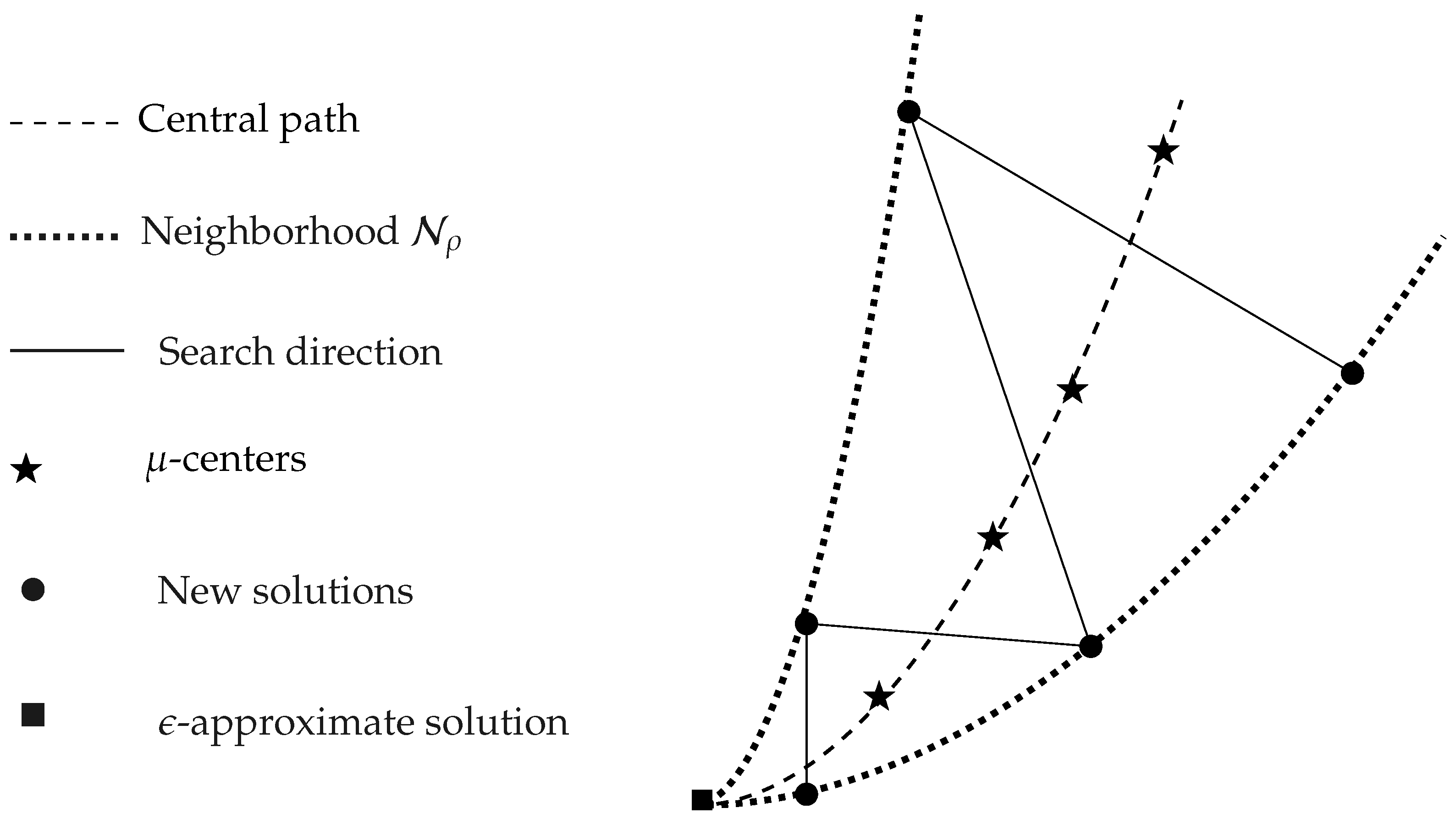
where $\mathit{e}=(1;1;\mathbf{0})$ is the identity vector of ${𝓡}^n$ as defined in Table 1, and $\delta \in (0,1)$ is a centering parameter that reduces the barrier term $\mu$. For any $\mu >0$, System (11) has a unique solution, indicated by $({\mathit{x}}_{\mu },{\mathit{y}}_{\mu },{\mathit{s}}_{\mu })$, where ${\mathit{x}}_{\mu }$ is called the $\mu$-center for (P) and the pair $({\mathit{y}}_{\mu },{\mathit{s}}_{\mu })$ is called the $\mu$-center for (D). The set of all $\mu$-centers that solve the perturbed KKT system (11) is called the central path of the pair (P, D), and is defined as

$$𝓒𝓟\triangleq \left\{({\mathit{x}}_{\mu },{\mathit{y}}_{\mu },{\mathit{s}}_{\mu })\in {𝓕}^0:\mathit{x}\circ \mathit{s}=\delta \mu \mathit{e},\mu >0\right\}.$$

Due the assumption that ${𝓕}^0\ne 0$, the central path is well defined. As $\mu$ gets closer to zero, the $\mu$-central point $({\mathit{x}}_{\mu },{\mathit{y}}_{\mu },{\mathit{s}}_{\mu })$ converges toward an $ϵ$-approximate solution $({\mathit{x}}^{★},{\mathit{y}}^{★},{\mathit{s}}^{★})$ of (P, D).

Now, we reformulate the complementary condition $\mathit{x}\circ \mathit{s}=\delta \mu \mathit{e}$ in (11), which is a direct consequence of Lemma 28 in [30].

Lemma 5. 

Let $\mathit{x},\mathit{s},\mathit{p}\in ({𝓡}^n,\circ ,•)$ be such that $\mathit{x},\mathit{s}\succ \mathbf{0}$, and $\mathit{p}$ is invertible (i.e., $det\left(\mathit{p}\right)\ne 0$). Then $\mathit{x}\circ \mathit{s}=\delta \mu \mathit{e}$ if and only if ${\mathrm{Q}}_{\mathit{p}}\mathit{x}\circ {\mathrm{Q}}_{{\mathit{p}}^{-1}}\mathit{s}=\delta \mu \mathit{e}$.

In order to solve System (11), we apply Newton’s method to this system and obtain

$$\begin{array}{cc}\hfill & 𝓐\mathrm{\Delta }\mathit{x}=\mathit{b}-𝓐\mathit{x},\hfill \\ \hfill & A^{\mathsf{T}}\mathrm{\Delta }\mathit{y}+\mathrm{\Delta }\mathit{s}=\mathit{c}-A^{\mathsf{T}}\mathit{y}-\mathit{s},\hfill \\ \hfill & {\mathrm{Q}}_{\mathit{p}}\mathit{x}\circ {\mathrm{Q}}_{{\mathit{p}}^{-1}}\mathrm{\Delta }\mathit{s}+{\mathrm{Q}}_{\mathit{p}}\mathrm{\Delta }\mathit{x}\circ {\mathrm{Q}}_{{\mathit{p}}^{-1}}\mathit{s}=\delta \mu \mathit{e}-{\mathrm{Q}}_{\mathit{p}}\mathit{x}\circ {\mathrm{Q}}_{{\mathit{p}}^{-1}}\mathit{s},\hfill \end{array}$$

(12)

where $(\mathrm{\Delta }\mathit{x},\mathrm{\Delta }\mathit{y},\mathrm{\Delta }\mathit{s})\in ({𝓡}^n,\circ ,•)\times R^m\times ({𝓡}^n,\circ ,•)$ is called the Newton search direction.

In the theory of Jordan algebra, two elements of a Jordan algebra operator commute if they share the same set of eigenvectors. In particular, two vectors $\mathit{u},\mathit{v}s.\in {𝓡}^n$ operator commute if ${\mathit{c}}_i={\mathit{c}}_i\left(\mathit{u}\right)={\mathit{c}}_i\left(\mathit{v}\right)$ for $i=1,2$, i.e., $\mathit{u}={\lambda }_1\left(\mathit{u}\right){\mathit{c}}_1+{\lambda }_2\left(\mathit{u}\right){\mathit{c}}_2$ and $\mathit{v}={\lambda }_1\left(\mathit{v}\right){\mathit{c}}_1+{\lambda }_2\left(\mathit{v}\right){\mathit{c}}_2$. The vectors $\mathit{x}$ and $\mathit{s}$ in System (12) may not operator commute. We need now to scale the underlying system so that the scaled vectors operator commute. In practice, this scaling is needed to guarantee that we iterate in the interior of the quadratic rotated cone.

Let $𝓒(\mathit{x},\mathit{s})$ be the set of nonsingular elements so that the scaled vectors operator commute, i.e.,

$$𝓒(\mathit{x},\mathit{s})=\left\{\mathit{p}\in {𝓡}^n:\mathit{p}\mathrm{nonsingular}\mathrm{and}{\mathrm{Q}}_{\mathit{p}}\mathit{x}\mathrm{and}{\mathrm{Q}}_{{\mathit{p}}^{-1}}\mathit{s}\mathrm{operator}\mathrm{commute}\right\}.$$

We call the set of directions $(\mathrm{\Delta }\mathit{x},\mathrm{\Delta }\mathit{y},\mathrm{\Delta }\mathit{s})$ arising by choosing $\mathit{p}$ from $𝓒(\mathit{x},\mathit{s})$ the commutative class of directions for RQCP, and call a direction in this class a commutative direction.

As mentioned earlier, the commutative class of primal-dual IPMs was designed by Monteiro and Zhang [29] for semidefinite programming, and by Alizadeh and Goldfarb [7] for second-order cone programming, and then extended by Schmieta and Alizadeh [30] for symmetric cone programming. We concentrate on three prominent choices of $\mathit{p}$, and each choice leads to a different direction in the commutative class of search directions: First, the choice $\mathit{p}={\mathit{s}}^{1/2}$ is referred to as the HRVW/KSH/M direction, and is equivalent to the XS direction in semidefinite programming (introduced by Helmberg, Rendl, Vanderbei, and Wolkowicz [31], and Kojima, Shindoh, and Hara [32] independently, and then rediscovered by Monteiro [29]). Second, the choice $\mathit{p}={\mathit{x}}^{-1/2}$ is referred to as the dual HRVW/KSH/M direction, and is equivalent to the SX direction in semidefinite programming. Third, the choice $\mathit{p}={\left({\mathrm{Q}}_{{\mathit{x}}^{1/2}}{\left({\mathrm{Q}}_{{\mathit{x}}^{1/2}}\mathit{s}\right)}^{-1/2}\right)}^{-1/2}={\left({\mathrm{Q}}_{{\mathit{s}}^{-1/2}}{\left({\mathrm{Q}}_{{\mathit{s}}^{1/2}}\mathit{x}\right)}^{1/2}\right)}^{-1/2}$ is equivalent to the NT direction in semidefinite programming (introduced by Nesterov and Todd [4]).

Now, associated with $\mathit{p}\in 𝓒(\mathit{x},\mathit{s})$, we make the following change of variables:

$$\begin{array}{cc}\hfill & \mathit{x}\to \overline{\mathit{x}}\triangleq {\mathrm{Q}}_{\mathit{p}}\mathit{x},\mathit{s}\to \underline{\mathit{s}}\triangleq {\mathrm{Q}}_{{\mathit{p}}^{-1}}\mathit{s},\mathit{c}\to \underline{\mathit{c}}\triangleq {\mathrm{Q}}_{{\mathit{p}}^{-1}}\mathit{c},A\to \underline{A}\triangleq A{\mathrm{Q}}_{{\mathit{p}}^{-1}},𝓐\to \underline{𝓐}\triangleq AH{\mathrm{Q}}_{{\mathit{p}}^{-1}}.\hfill \end{array}$$

Because ${\mathrm{Q}}_{{\mathit{p}}^{-1}}={\mathrm{Q}}_{\mathit{p}}^{-1}$ (see [28], Theorem 4.3), System (12) is equivalent to

$$\begin{array}{ccc}\hfill \underline{𝓐}\overline{\mathrm{\Delta }\mathit{x}}& =\hfill & {\mathit{r}}_{\mathrm{p}},\hfill \\ \hfill {\underline{A}}^{\mathsf{T}}\mathrm{\Delta }\mathit{y}+\underline{\mathrm{\Delta }\mathit{s}}& =\hfill & {\mathit{r}}_{\mathrm{d}},\hfill \\ \hfill \overline{\mathit{x}}\circ \underline{\mathrm{\Delta }\mathit{s}}+\overline{\mathrm{\Delta }\mathit{x}}\circ \underline{\mathit{s}}& =\hfill & {\mathit{r}}_{\mathrm{c}},\hfill \end{array}\mathrm{or}\mathrm{equivalently}\left[\begin{array}{ccc}\underline{𝓐}& \mathbf{O}& \mathbf{O}\\ \mathbf{O}& {\underline{A}}^{\mathsf{T}}& I\\ \mathrm{L}\left(\underline{\mathit{s}}\right)& \mathbf{O}& \mathrm{L}\left(\overline{\mathit{x}}\right)\end{array}\right]\left[\begin{array}{c}\overline{\mathrm{\Delta }\mathit{x}}\\ \mathrm{\Delta }\mathit{y}\\ \underline{\mathrm{\Delta }\mathit{s}}\end{array}\right]=\left[\begin{array}{c}{\mathit{r}}_{\mathrm{p}}\\ {\mathit{r}}_{\mathrm{d}}\\ {\mathit{r}}_{\mathrm{c}}\end{array}\right],$$

(13)

where ${\mathit{r}}_{\mathrm{p}},{\mathit{r}}_{\mathrm{d}}$, and ${\mathit{r}}_{\mathrm{c}}$ are given by

$${\mathit{r}}_{\mathrm{p}}\triangleq \mathit{b}-\underline{𝓐}\overline{\mathit{x}},{\mathit{r}}_{\mathrm{d}}\triangleq \underline{\mathit{c}}-{\underline{A}}^{\mathsf{T}}\mathit{y}-\underline{\mathit{s}},{\mathit{r}}_{\mathrm{c}}\triangleq \delta \mu \mathit{e}-\overline{\mathit{x}}\circ \underline{\mathit{s}}.$$

Applying block Gaussian elimination to (13), we obtained the Newton search directions $(\overline{\mathrm{\Delta }\mathit{x}},\mathrm{\Delta }\mathit{y},\underline{\mathrm{\Delta }\mathit{s}})$:

$$\begin{array}{ccc}\overline{\mathrm{\Delta }\mathit{x}}\hfill & =\hfill & {\mathrm{L}}^{-1}\left(\underline{\mathit{s}}\right)\left({\mathit{r}}_{\mathrm{c}}-\mathrm{L}\left(\overline{\mathit{x}}\right)\underline{\mathrm{\Delta }\mathit{s}}\right),\hfill \\ \mathrm{\Delta }\mathit{y}\hfill & =\hfill & {\left(\underline{𝓐}{\mathrm{L}}^{-1}\left(\underline{\mathit{s}}\right)\mathrm{L}\left(\overline{\mathit{x}}\right){\underline{A}}^{\mathsf{T}}\right)}^{-1}\left({\mathit{r}}_{\mathrm{p}}+\underline{𝓐}{\mathrm{L}}^{-1}\left(\underline{\mathit{s}}\right)(\mathrm{L}\left(\overline{\mathit{x}}\right){\mathit{r}}_{\mathrm{d}}-{\overline{r}}_{\mathrm{c}})\right),\hfill \\ \underline{\mathrm{\Delta }\mathit{s}}\hfill & =\hfill & {\mathit{r}}_{\mathrm{d}}-{\underline{A}}^{\mathsf{T}}\overline{\mathrm{\Delta }\mathit{y}}.\hfill \end{array}$$

To obtain the search directions $\mathrm{\Delta }\mathit{x}$ and $\mathrm{\Delta }\mathit{s}$ for (12), we apply inverse scaling to $\overline{\mathrm{\Delta }\mathit{x}}$ and $\underline{\mathrm{\Delta }\mathit{s}}$ as follows:

$$\mathrm{\Delta }\mathit{x}\triangleq {\mathrm{Q}}_{{\mathit{p}}^{-1}}\overline{\mathrm{\Delta }\mathit{x}}\mathrm{and}\mathrm{\Delta }\mathit{s}\triangleq {\mathrm{Q}}_{\mathit{p}}\underline{\mathrm{\Delta }\mathit{s}}.$$

Finally, we take a step size $\alpha$ so that the new point $({\mathit{x}}^{+},{\mathit{y}}^{+},{\mathit{s}}^{+})\triangleq (\mathit{x},\mathit{y},\mathit{s})+\alpha (\mathrm{\Delta }\mathit{x},\mathrm{\Delta }\mathit{y},\mathrm{\Delta }\mathit{s})$ is generated in the neighborhood of the central path; see Figure 1.

5. Path-Following Interior-Point Algorithms

Primal–dual path-following IPMs for solving the pair (P, D) are introduced in this section in three different lengths: short, semi-long, and long-step.

The generation of each iteration $({\mathit{x}}_{\mu }^{\left(k\right)},{\mathit{y}}_{\mu }^{\left(k\right)},{\mathit{s}}_{\mu }^{\left(k\right)})$ in the neighborhood of the central path $𝓒𝓟$ is one of the main issues in the path-following IPMs, and we use proximity measure functions to handle this. With our adherence to the central path, the duality gap sequence $\left\{{\mu }_k\right\}$ will converge, and a bound on the number of iterations needed to obtain the optimal solution of the pair problem (P, D) will be polynomial.

The standard way to classify the proximity measures is to measure the distance to a specific point on the central path $𝓒𝓟$. More specifically, the proximity measures for $\mathit{x},\mathit{s}\succ \mathbf{0}$ are given as

$$\begin{array}{ccc}{d}_{\mathrm{F}}(\mathit{x},\mathit{s})\hfill & \triangleq \hfill & \parallel {\mathrm{Q}}_{{\mathit{x}}^{1/2}}\mathit{s}-\mu \mathit{e}{\}\parallel }_{\mathrm{F}}=\sqrt{{\lambda }_1{({\mathrm{Q}}_{{\mathit{x}}^{1/2}}\mathit{s}-\mu )}^2+{\lambda }_2{({\mathrm{Q}}_{{\mathit{x}}^{1/2}}\mathit{s}-\mu )}^2},\hfill \\ d_2(\mathit{x},\mathit{s})\hfill & \triangleq \hfill & \parallel {\mathrm{Q}}_{{\mathit{x}}^{1/2}}\mathit{s}-\mu \mathit{e}{\}\parallel }_2=max\{\left|{\lambda }_1\left({\mathrm{Q}}_{{\mathit{x}}^{1/2}}\mathit{s}\right)-\mu \right|,\left|{\lambda }_2\left({\mathrm{Q}}_{{\mathit{x}}^{1/2}}\mathit{s}\right)-\mu \right|\},\hfill \\ d_{-\infty }(\mathit{x},\mathit{s})\hfill & \triangleq \hfill & \mu -{\lambda }_{min}\left({\mathrm{Q}}_{{\mathit{x}}^{1/2}}\mathit{s}\right)=\mu -min\{{\lambda }_1\left({\mathrm{Q}}_{{\mathit{x}}^{1/2}}\mathit{s}\right),{\lambda }_2\left({\mathrm{Q}}_{{\mathit{x}}^{1/2}}\mathit{s}\right)\}.\hfill \end{array}$$

(14)

The three different distances in (14) lead to the following three neighborhoods along the central path:

$$\begin{array}{ccc}{𝓝}_{\mathrm{F}}\left(\gamma \right)\hfill & \triangleq \hfill & \left\{(\mathit{x},\mathit{y},\mathit{s})\in {𝓕}^{\circ }:d_{\mathrm{F}}(\mathit{x},\mathit{s})\le \gamma \mu \right\},\hfill \\ {𝓝}_2\left(\gamma \right)\hfill & \triangleq \hfill & \left\{(\mathit{x},\mathit{y},\mathit{s})\in {𝓕}^{\circ }:d_2(\mathit{x},\mathit{s})\le \gamma \mu \right\},\hfill \\ {𝓝}_{-\infty }\left(\gamma \right)\hfill & \triangleq \hfill & \left\{(\mathit{x},\mathit{y},\mathit{s})\in {𝓕}^{\circ }:d_{-\infty }(\mathit{x},\mathit{s})\le \gamma \mu \right\},\hfill \end{array}$$

(15)

where $\gamma \in (0,1)$ is a constant known as the neighborhood parameter.

By Proposition 21 in [30], both ${\mathrm{Q}}_{{\mathit{x}}^{1/2}}\mathit{s}$ and ${\mathrm{Q}}_{{\overline{\mathit{x}}}^{1/2}}\underline{\mathit{s}}$ have the same eigenvalues, and since all neighborhoods ${𝓝}_{\rho }\left(\gamma \right)$ may be described in terms of the eigenvalue of ${\mathrm{Q}}_{{\mathit{x}}^{1/2}}\mathit{s}$, one can see that the neighborhoods defined in (15) are scaling-invariant, i.e., $(\mathit{x},\mathit{s})\in {𝓝}_{\rho }\left(\gamma \right)\mathrm{if}\mathrm{and}\mathrm{only}\mathrm{if}(\overline{\mathit{x}},\underline{\mathit{s}})\in {𝓝}_{\rho }\left(\gamma \right),$ where $\rho$ can be selected as $F,2$, or $-\infty$.

Furthermore, given the eigenvalue characterization of $d_{\rho }(\mathit{x},\mathit{s})$, we can find that $d_{-\infty }(\mathit{x},\mathit{s})\le d_2(\mathit{x},\mathit{s})\le d_{\mathrm{F}}(\mathit{x},\mathit{s})$, and hence ${𝓝}_{\mathrm{F}}\left(\gamma \right)\subseteq {𝓝}_2\left(\gamma \right)\subseteq {𝓝}_{-\infty }\left(\gamma \right).$

The performance of the path-following IPMs for RQCP problems greatly depends on the neighborhood ${𝓝}_{\rho }\left(\gamma \right)$ of the central path and the centering parameter $\delta$ that we select. These options allow us to divide the path-following IPMs for our problem into three categories: Short, semi-long, and long-step. More specifically:

• Selecting ${𝓝}_{\mathrm{F}}\left(\gamma \right)$ as the neighborhood yields the short-step algorithm;
• Selecting ${𝓝}_2\left(\gamma \right)$ as the neighborhood yields the semi-long-step algorithm;
• Selecting ${𝓝}_{-\infty }\left(\gamma \right)$ as the neighborhood yields the long-step algorithm.

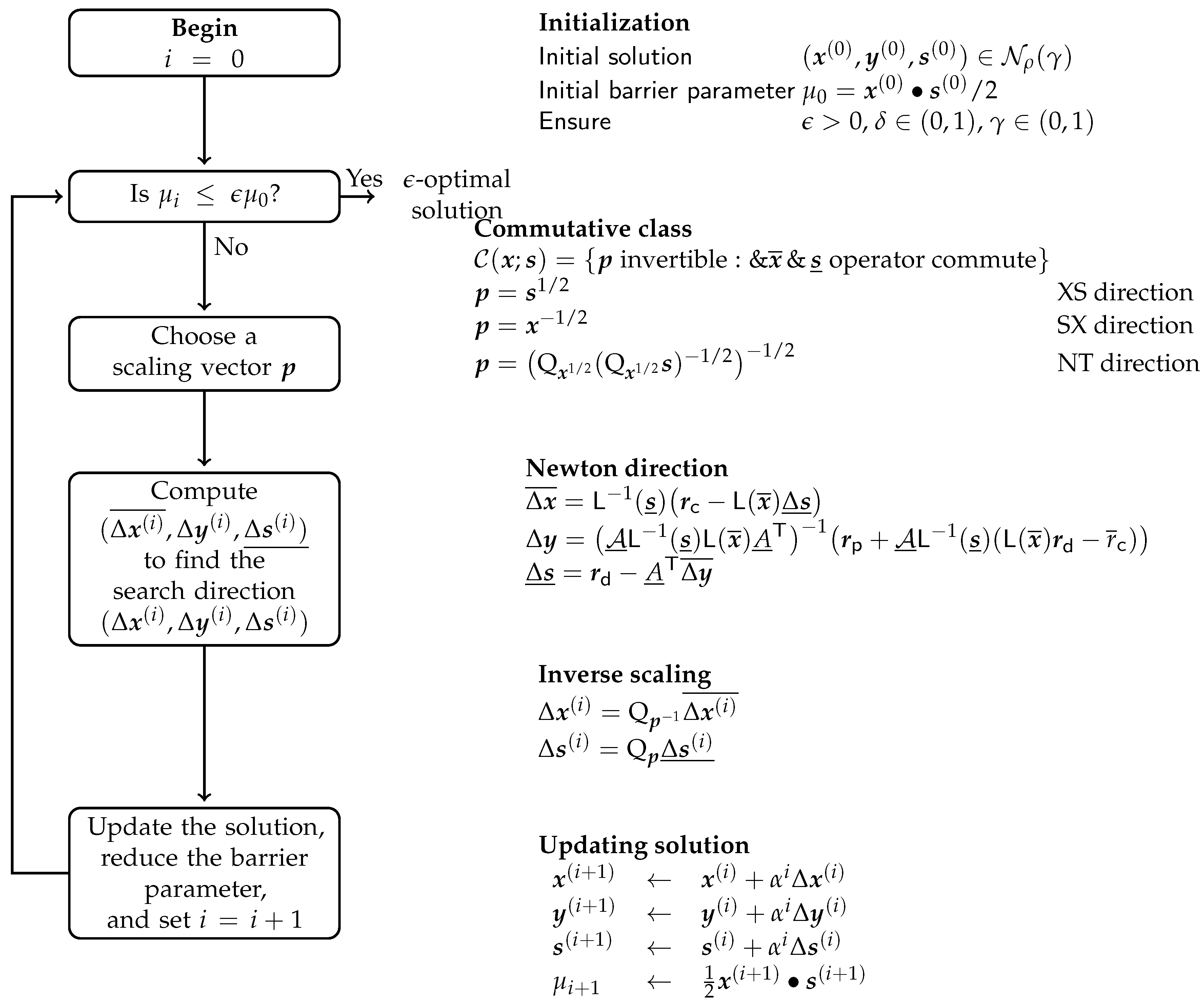
We indicate that the long-step version of the algorithm seems to outperform the short-step version of the algorithm in practical performance. In

Table 2. Contrasting some features of path-following IPMs in short, semi-long, and long-step versions.

Features	Short-Step Algorithm	Semi-Long-Step Algorithm	Long-Step Algorithm
Neighborhood ${𝓝}_{\rho }\left(\gamma \right)$	${𝓝}_{\mathrm{F}}\left(\gamma \right)$	${𝓝}_{-\infty }\left(\gamma \right)$	${𝓝}_2\left(\gamma \right)$
Factor $\sigma$	$(0,1)$	$(0,1)$	$(0,1)$
Centering parameter $\delta$	$1-\sigma /\sqrt{2r}$	$(0,1)$	$(0,1)$
No. of iter. in NT direction	$𝓞(\sqrt{2r}log(1/ϵ))$	$𝓞(2rlog(1/ϵ\left)\right)$	$𝓞(2rlog(1/ϵ\left)\right)$
No. of iter. in HRVW/KSH/M	$𝓞(\sqrt{2r}log(1/ϵ))$	$𝓞(2rlog(1/ϵ\left)\right)$	$𝓞({\left(2r\right)}^{3/2}log(1/ϵ))$
direction or its dual

, we compare some of the categorized versions of this algorithm. The proposed path-following interior-point algorithm for solving the pair of problems (P, D) is described in Algorithm 1 and Figure 2.

Algorithm 1: A path-following interior algorithm for solving RQCP problem.

The convergence and time complexity for Algorithm 1 is given in the following theorem. This theorem is a consequence of Theorem 1 that we verified in Section 2 and Theorem 37 in [30] after taking the rotated quadratic cone ${𝓡}_{+}^n$ as our underlying symmetric cone.

Theorem 3. 

If each iteration in Algorithm 1 follows the NT direction, then the short-step algorithm terminates in $𝓞({\left(2r\right)}^{1/2}log(1/ϵ))$ iterations, and the semi-long and long-step algorithms terminate in $𝓞(2rlog(1/ϵ\left)\right)$ iterations. If each iteration in Algorithm 1 follows the HRVW/KSH/M direction or dual HRVW/KSH/M direction, then the short-step algorithm terminates in $𝓞({\left(2r\right)}^{1/2}log(1/ϵ))$ iterations, the semi-long-step algorithm terminates in $𝓞(2rlog(1/ϵ\left)\right)$ iterations, and the long-step algorithm terminates in $𝓞({\left(2r\right)}^{3/2}log(1/ϵ))$ iterations.

Before closing this section and moving forward to our numerical results below, we indicate that the above analysis can be carried out and extended word-by-word if Problem (P, D) is given in multiple block-setting by using the notations introduced in Table 1.

6. Numerical Results

In this section, we will assess how well the proposed method performs when implemented to some RQCP problems: The problem of minimizing the harmonic mean of positive affine function, and some randomly generating problems. We also contrast the numerical results of the proposed algorithm for the randomly generated problems with those of the two symmetric cone programming software package systems: CVX [33] and MOSEK [34].

We produced our numerical results using MATLAB version R2021a on a PC with an Intel (R) Core (TM) i3-1005G1 processor operating at 1.20 GHz and 4 GB of physical memory. In the first numerical example, we consider a problem in multiple block setting. The dimensions of our test problems are denoted by the letters m and n, and the number of block splittings is denoted by r. “Iter” stands for the typical number of iterations needed to obtain $ϵ$-optimal solutions, while “CPU” stands for the typical CPU time needed to reach an $ϵ$-optimal solution to the underlying problem.

In all of our tests, we use the long-step path-following version of Algorithm 1, and choose the dual HRVW/KSH/M direction (i.e., our scaling vector is $\mathit{p}={\mathit{x}}^{-1/2}$). Furthermore, when the condition of convergence is not satisfied at an iteration step, it will generate a new solution that must be in the neighborhood of the central path. We choose the step size of $\alpha$ that was proposed in [30].

Example 1 

(Minimizing the harmonic mean of affine functions). We consider the problem of minimizing the harmonic mean of (positive) affine functions of $\mathit{x}\in {\mathbb{R}}^n$ [7]:

$$\begin{array}{ccccc}min\hfill & {\displaystyle \sum _{i=1}^r\frac{1}{{\mathit{a}}_i^{\mathsf{T}}\mathit{x}+{\beta }_i}}\hfill & & min\hfill & {\displaystyle \sum _{i=1}^r{u}_i}\hfill \\ \mathrm{s}.\mathrm{t}.\hfill & {\mathit{a}}_i^{\mathsf{T}}\mathit{x}+{\beta }_i>0,i=1,2,\cdots ,r,\hfill & \mathit{which}\mathit{can}\mathit{be}\mathit{cast}\mathit{as}\hfill & s.t.\hfill & u_i({\mathit{a}}_i^{\mathsf{T}}\mathit{x}+{\beta }_i)\ge 1,i=1,2,\cdots ,r,\hfill \\ & {\mathit{d}}_j^{\mathsf{T}}\mathit{x}+h_j\ge 0,j=1,2,\cdots ,m;\hfill & \mathit{the}\mathit{RQCP}\mathit{problem}\hfill & & u_i\ge 0,i=1,2,\cdots ,r,\hfill \\ & & & & {\mathit{d}}_j^{\mathsf{T}}\mathit{x}+h_j\ge 0,j=1,2,\cdots ,m.\hfill \end{array}$$

We implement this problem for sizes $n=6,12,24,30,36$, $m=3,9,15$, and the number of blocks $r=5,10,15,20$. We generate the coefficients ${\mathit{a}}_i,{\beta }_i,{\mathit{d}}_j$ and $h_j$ randomly from a list of numbers uniformly distributed between −1 and 1 for all $i=1,2,\cdots ,r$ and $j=1,2,\cdots ,m$. We take the parameters $ϵ={10}^{-6}$, $\sigma =0.55$, and $\gamma =0.8$. The initial solutions of ${\mathit{x}}^{\left(0\right)},{\mathit{s}}^{\left(0\right)}$ are also chosen randomly from a list of uniformly distributed numbers between −1 and 1, while ${\mathit{y}}^{\left(0\right)}$ is chosen as the zero vector, and $u_i,i=1,2,\cdots ,r$, are all set to take values between 0 and 1. We display the numerical results obtained for this example in

Table 3. The numerical results obtained for minimizing harmonic mean of affine functions in Example 1.

m	n	r		Iter.	CPU(s)		m	n	r		Iter.	CPU(s)		m	n	r		Iter.	CPU(s)
3	6	5		2	0.0156		9	6	5		8	0.1562		15	6	5		32	0.4062
3	6	10		4	0.0781		9	6	10		16	0.0781		15	6	10		42	0.3125
3	6	15		5	0.1094		9	6	15		20	0.4844		15	6	15		44	0.5781
3	6	20		5	0.1562		9	6	20		15	0.5938		15	6	20		57	0.4844
3	12	5		5	0.0312		9	12	5		24	0.1094		15	12	5		27	0.5406
3	12	10		7	0.1094		9	12	10		27	0.2188		15	12	10		32	0.5546
3	12	15		8	0.2031		9	12	15		27	0.4804		15	12	15		24	0.7679
3	12	20		11	0.2931		9	12	20		32	0.5000		15	12	20		31	0.5932
3	24	5		11	0.1719		9	24	5		22	0.1875		15	24	5		36	0.5381
3	24	10		15	0.2500		9	24	10		25	0.2969		15	24	10		31	0.8344
3	24	15		16	0.1562		9	24	15		29	0.3750		15	24	15		52	0.9306
3	24	20		19	0.3901		9	24	20		33	0.5156		15	24	20		49	0.8656
3	30	5		16	0.1904		9	30	5		23	0.1875		15	30	5		40	0.6265
3	30	10		20	0.1406		9	30	10		39	0.2969		15	30	10		44	0.9018
3	30	15		23	0.2812		9	30	15		23	0.2344		15	30	15		49	0.8031
3	30	20		26	0.3112		9	30	20		41	0.5469		15	30	20		54	0.8750
3	36	5		32	0.3938		9	36	5		28	0.1719		15	36	5		52	0.6925
3	36	10		19	0.2998		9	36	10		35	0.3906		15	36	10		54	0.7562
3	36	15		34	0.3438		9	36	15		39	0.3438		15	36	15		69	0.7906
3	36	20		26	0.5469		9	36	20		47	0.3125		15	36	20		72	0.9789

, and visualize them graphically in Figure 3.

Example 2 

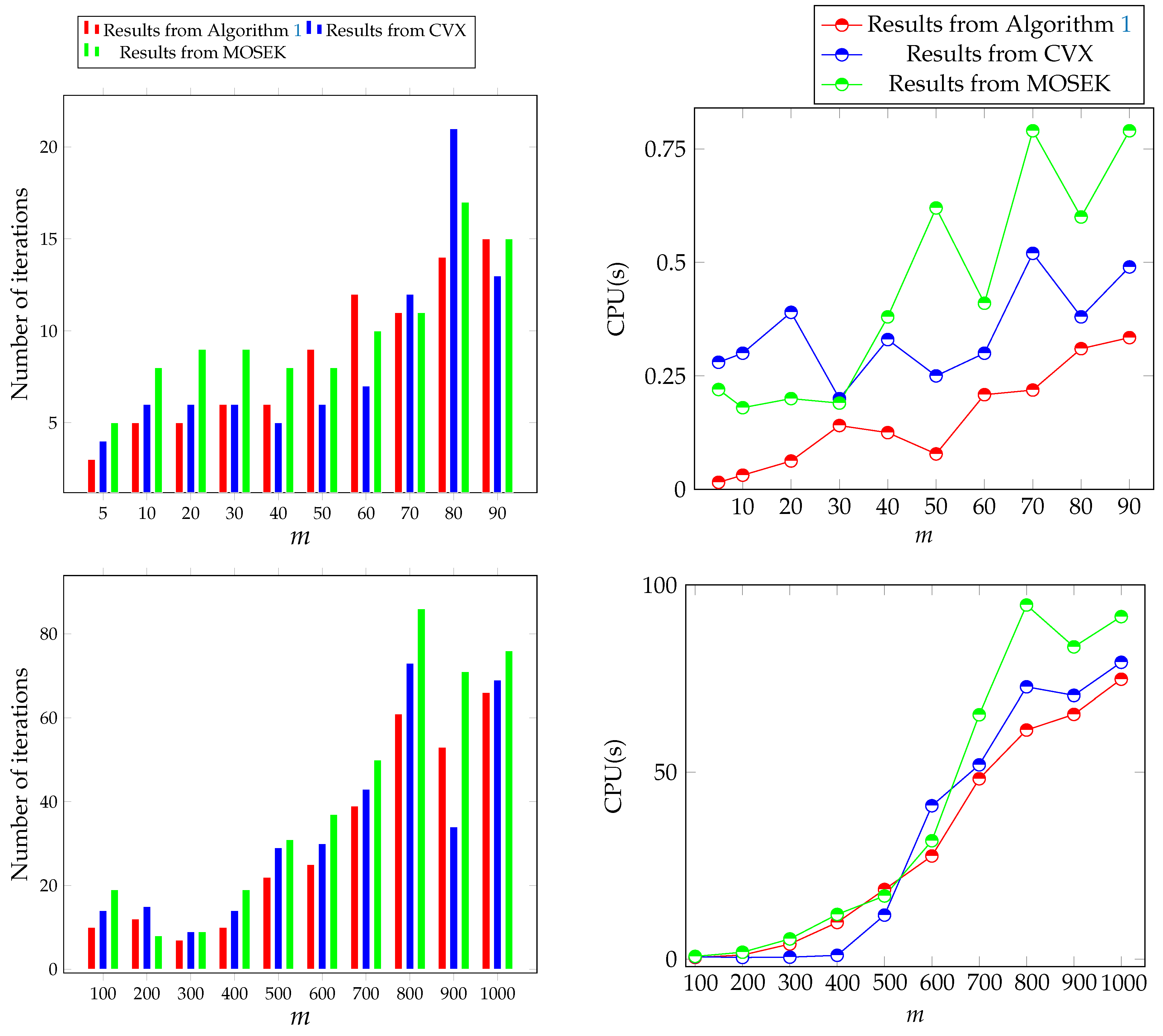
(Randomly generated problems). In this example, the coefficients A and b are generated at random from a list of uniformly distributed numbers between −1 and 1. We set $\mathit{b}=𝓐{\mathit{x}}^{\left(0\right)}$ and $\mathit{c}=A^{\mathsf{T}}{\mathit{y}}^{\left(0\right)}+{\mathit{s}}^{\left(0\right)}$, and choose the parameters $ϵ={10}^{-4}$, $\sigma =0.33$ and $\gamma =0.9$. The size of the problem is given so that $n=2m$, where m is ranging from 5 to 1000. The initial solutions are chosen as follows: ${\mathit{x}}^{\left(0\right)}=\mathit{e}$, ${\mathit{s}}^{\left(0\right)}=\mathit{e}$ and ${\mathit{y}}^{\left(0\right)}=\mathbf{0}$. We display our numerical results in

Table 4. The numerical results obtained for the randomly generated problems in Example 2.

Problem Size	Algorithm 1		CVX		MOSEK
$(\mathit{m},\mathit{n})$	Iter.	CPU(s)	Iter.	CPU(s)	Iter.	CPU(s)
(5, 10)	3	0.0156	4	0.28	5	0.22
(10, 20)	5	0.0313	6	0.30	8	0.18
(20, 40)	5	0.0625	6	0.39	9	0.20
(30, 60)	6	0.1406	6	0.20	9	0.19
(40, 80)	6	0.1250	5	0.33	8	0.38
(50, 60)	9	0.0781	6	0.25	8	0.62
(60, 120)	12	0.2086	7	0.30	10	0.41
(70, 140)	11	0.2188	12	0.52	11	0.79
(80,160)	14	0.3100	21	0.38	17	0.60
(90, 180)	15	0.3343	13	0.49	15	0.79
(100, 200)	10	0.4531	14	0.66	19	0.74
(200, 400)	12	1.0900	15	0.44	8	1.85
(300,600)	7	4.0313	9	0.53	9	5.41
(400, 800)	10	9.804	14	1.02	19	11.97
(500, 1000)	22	18.6406	29	11.78	31	16.90
(600, 1200)	25	27.5938	30	41.03	37	31.67
(700, 1400)	39	48.2500	43	51.97	50	65.36
(800, 1600)	61	61.2813	73	72.77	86	94.64
(900, 1800)	53	65.4651	34	70.50	71	83.45
(1000, 2000)	66	74.7968	69	79.32	76	91.54

, and visualize them graphically in Figure 4. The results from the CVX and MOSEK solvers are also presented in Table 4 and Figure 4 for comparison purposes.

We can see overall that the computational results show that Algorithm 1 performs well in practice. We can see from the numerical results shown in Table 3 and Table 4 and represented in Figure 3 and Figure 4 that the number of iterations and CPU time required by Algorithm 1 increase as the dimension of the underlying problem increases, indicating that the dimension of the problem and the dimension of rotated quadratic cones have an impact on the number of iterations and the amount of time required by the proposed algorithm. Furthermore, when the randomly generated problems are solved using the CVX and Mosek solvers, we can see that most of the solutions exhibited a slight bias toward Algorithm 1 in terms of both the number of iterations and CPU time. This is most likely because these solvers begin at infeasible points or because the stopping condition of the algorithm used in these solvers differs from that of Algorithm 1.

7. Concluding Remarks

All earlier work on optimization problems over the rotated quadratic cones has formulated these problems as second-order cone programming problems, and while doing this can be easier than developing special-purpose algorithms for solving this class of optimization problems, this approach may not always be the cheapest one in terms of computational cost. In this paper, we have introduced the rotated quadratic cone programming problems as a “self-made” class of optimization problems. We have proved that the barrier function associated with our cone is strongly self-concordant. We have discussed the duality theory associated with these problems, along with the development of the commutative class of search directions, and have developed a primal–dual interior-point algorithm rotated quadratic cone optimization problems based on our own Euclidean Jordan algebra. The efficiency of the proposed algorithm is shown by providing some numerical examples and comparing some of them with results from MOSEK and CVX solvers.

The proposed algorithm is attractive from an algebraic point of view. Most of this attractiveness comes from exploiting the algebraic structure of the quadratic rotated cone which allowed us to explicitly give expressions for the inverse operator, the linear representation, and the quadratic operator, and use these operators to compute the derivatives of the barrier function explicitly. In spite of its attractiveness, the algorithm has several limitations such as producing a good starting point, developing a practical step length selection procedure in the primal space, and reducing the barrier parameter with a practical strategy in our setting. These limitations, however, could be addressed in a future research paper developing practical implementations. Future work can be performed on developing algorithms for solving mixed-integer rotated quadratic cone optimization problems.

References

- Montoya, O.; Gil-González, W.; Garcés, A. On the conic convex approximation to locate and size fixed-step capacitor banks in distribution networks. Computation 2022, 10, 32. [Google Scholar] [CrossRef]
- Alzalg, B. A primal-dual interior-point method based on various selections of displacement step for symmetric optimization. Comput. Optim. Appl. 2019, 72, 363–390. [Google Scholar] [CrossRef]
- Nesterov, Y.; Nemirovskii, A. Interior-Point Polynomial Algorithms in Convex Programming; SIAM: Philadelphia, PA, USA, 1994. [Google Scholar]
- Nesterov, Y.E.; Todd, M.J. Self-scaled barriers and interior-point methods for convex programming. Math. Oper. Res. 1997, 22, 1–42. [Google Scholar] [CrossRef] [Green Version]
- Manshadi, S.D.; Liu, G.; Khodayar, M.E.; Wang, J.; Dai, R. A convex relaxation approach for power flow problem. J. Mod. Power Syst. Clean Energy 2019, 7, 1399–1410. [Google Scholar] [CrossRef] [Green Version]
- Manshadi, S.D.; Liu, G.; Khodayar, M.E.; Wang, J.; Dai, R. A distributed convex relaxation approach to solve the power flow problem. IEEE Syst. J. 2019, 14, 803–812. [Google Scholar] [CrossRef]
- Alizadeh, F.; Goldfarb, D. Second-order cone programming. Math. Program. 2003, 95, 3–51. [Google Scholar] [CrossRef]
- Alzalg, B.; Pirhaji, M. Elliptic cone optimization and primal–dual path-following algorithms. Optimization 2017, 66, 2245–2274. [Google Scholar] [CrossRef]
- Malakar, S.; Ghosh, M.; Bhowmik, S.; Sarkar, R.; Nasipuri, M. A GA based hierarchical feature selection approach for handwritten word recognition. Neural. Comput. Appl. 2020, 32, 2533–2552. [Google Scholar] [CrossRef]
- Bacanin, N.; Stoean, R.; Zivkovic, M.; Petrovic, A.; Rashid, T.A.; Bezdan, T. Performance of a novel chaotic firefly algorithm with enhanced exploration for tackling global optimization problems: Application for dropout regularization. Mathematics 2021, 9, 2705. [Google Scholar] [CrossRef]
- Tuba, E.; Bacanin, N. An algorithm for handwritten digit recognition using projection histograms and SVM classifier. In Proceedings of the 2015 23rd Telecommunications Forum Telfor (TELFOR), Belgrade, Serbia, 24–26 November 2015; pp. 464–467. [Google Scholar]
- Karmarkar, N. A new polynomial-time algorithm for linear programming. In Proceedings of the Sixteenth Annual ACM Symposium on Theory of Computing, Washington, DC, USA, 30 April–2 May 1984; pp. 302–311. [Google Scholar]
- Güler, O. Barrier functions in interior point methods. Math. Oper. Res. 1996, 21, 860–885. [Google Scholar] [CrossRef] [Green Version]
- Faraut, J. Analysis on Symmetric Cones; Oxford Mathematical Monographs: Oxford, UK, 1994. [Google Scholar]
- Todd, M. Semidefinite optimization. Acta Numer. 2001, 10, 515–560. [Google Scholar] [CrossRef] [Green Version]
- Alzalg, B. Combinatorial and Algorithmic Mathematics: From Foundation to Optimization; Kindle Direct Publishing: Seattle, WA, USA, 2022. [Google Scholar]
- Alzalg, B. Homogeneous self-dual algorithms for stochastic second-order cone programming. J. Optim. Theory Appl. 2014, 163, 148–164. [Google Scholar] [CrossRef]
- Alzalg, B. Volumetric barrier decomposition algorithms for stochastic quadratic second-order cone programming. Appl. Math. Comput. 2015, 265, 494–508. [Google Scholar] [CrossRef]
- Alzalg, B. A logarithmic barrier interior-point method based on majorant functions for second-order cone programming. Optim. Lett. 2020, 14, 729–746. [Google Scholar] [CrossRef]
- Alzalg, B.; Badarneh, K.; Ababneh, A. An infeasible interior-point algorithm for stochastic second-order cone optimization. J. Optim. Theory Appl. 2019, 181, 324–346. [Google Scholar] [CrossRef]
- Alzalg, B.; Gafour, A.; Alzaleq, L. Volumetric barrier cutting plane algorithms for stochastic linear semi-infinite optimization. IEEE Access 2019, 8, 4995–5008. [Google Scholar] [CrossRef]
- Alzalg, B.; Pirhaji, M. Primal-dual path-following algorithms for circular programming. Commun. Comb. Optim. 2017, 2, 65–85. [Google Scholar]
- Kojima, M.; Mizuno, S.; Yoshise, A. A primal-dual interior point algorithm for linear programming. In Progress in Math. Program; Springer: New York, NY, USA, 1989; pp. 29–47. [Google Scholar]
- Monteiro, R.D.; Adler, I. Interior Path Following Primal-Dual Algorithms. Part I: Linear Programming. Math. Program. 1989, 44, 27–41. [Google Scholar] [CrossRef]
- Alzalg, B. Primal interior-point decomposition algorithms for two-stage stochastic extended second-order cone programming. Optimization 2018, 67, 2291–2323. [Google Scholar] [CrossRef]
- Goldfarb, D.; Liu, S. An O(n3L) Primal interior point algorithm for convex quadratic programming. Math. Program. 1991, 49, 325–340. [Google Scholar] [CrossRef]
- Tiande, G.; Shiquan, W. Properties of primal interior point methods for QP. Optimization 1996, 37, 227–238. [Google Scholar] [CrossRef]
- Alzalg, B.; Tamsaouete, K.; Benakkouche, L.; Ababneh, A. The Jordan Algebraic Structure of the Rotated Quadratic Cone. Submitted for Publication. 2017. Available online: https://optimization-online.org/wp-content/uploads/2023/01/RQC.pdf (accessed on 31 January 2023).
- Monteiro, R.D.C.; Zhang, Y. A unified analysis for a class of path-following primal-dual interior-point algorithms for semidefinite programming. Math. Program. 1998, 81, 281–299. [Google Scholar] [CrossRef] [Green Version]
- Schmieta, S.H.; Alizadeh, F. Extension of primal-dual interior point algorithms to symmetric cones. Math. Program. 2003, 96, 409–438. [Google Scholar] [CrossRef]
- Helmberg, C.; Rendl, F.; Vanderbei, R.J.; Wolkowicz, H. An interior-point method for semidefinite programming. SIAM J. Optim. 1996, 6, 342–361. [Google Scholar] [CrossRef]
- Kojima, M.; Shindoh, S.; Hara, S. Interior-point methods for the monotone semidefinite linear complementarity problem in symmetric matrices. SIAM J. Optim. 1997, 7, 86–125. [Google Scholar] [CrossRef]
- Grant, M.; Boyd, S.; Ye, Y. CVX: Matlab Software for Disciplined Convex Programming (Webpage and Software); CVX Research, Inc.: Austin, TX, USA, 2009. [Google Scholar]
- Mosek ApS. Mosek Optimization Toolbox for Matlab. In User’s Guide and Reference Manual; Version 4; Mosek ApS: Copenhagen, Denmark, 2019. [Google Scholar]
Figure 1.
The alteration between steps to follow the central path.
Figure 2.
A pseudocode for Algorithm 1.
Figure 3.
Dot plots of the numerical results obtained in Example 1.
Figure 4.
Two-dimensional plots for the numerical results in Example 2.