
Numerical Study on Surface Reconstruction and Roughness of Magnetorheological Elastomers

1
PCM Computational Applications, Department of Physics, Universidad Nacional de Colombia, Campus La Nubia, Manizales 170003, Colombia
2
Group of Magnetism and Simulation G+, Institute of Physics, Universidad de Antioquia, Medellín 050010, Colombia
*
Author to whom correspondence should be addressed.
Computation 2023, 11(3), 46; https://doi.org/10.3390/computation11030046
Submission received: 8 November 2022
/
Revised: 13 January 2023
/
Accepted: 18 January 2023
/
Published: 27 February 2023
(This article belongs to the Topic Advances in Computational Materials Sciences)
Abstract
:A methodology is implemented to deform the surface of a magnetorheological elastomer (MRE) exposed to an external magnetic field by means of data matrix manipulation of the surface. The elastomer surface is created randomly using the Garcia and Stoll method to realize a nonuniform morphology similar to that found in real MREs. Deformations are induced by means of the translations of the magnetic particles inside the elastomer, under the influence of a uniform magnetic field, generating changes in the surface roughness. Our model computes these deformations using a three-dimensional Gaussian function bounded at 2 standard deviations from its mean value, taking as the standard deviation value the radius of the particle that causes the deformation. To find the regions deformed by the particles, we created a methodology based on the consultation, creation and modification of a system of matrices that control each point of the random surface created. This methodology allows us to work with external files of initial and subsequent positions of each particle inside the elastomer, and allows us to manipulate and analyze the results in a smoother and faster way. Results were found to be satisfactory and consistent when calculating the percentage of surface deformation of real systems.
1. Introduction
Magnetorheological elastomers (MRE) are materials composed of an elastic material known as elastomer (for example polydimethylsiloxane or PDMS, silicone rubber, natural rubbe, butadiene rubber polyurethane, etc. [1]) along with embedded magnetic particles, so that the material can be deformed by the influence of an external magnetic field. These materials can be divided into two groups: isotropic MRE and anisotropic MRE. The former are exposed to a magnetic field at the time of curing, obtaining a chain-like arrangement of the magnetic particles inside, whereas the latter are not exposed to a magnetic field at the time of curing, obtaining a random distribution of the particles inside [2,3]. When an MRE is immersed in an external magnetic field, the particles are magnetized, resulting in a dipolar interaction among them, forming chains of particles. The movements of theses particles within the elastomer matrix cause deformations, mostly evidenced on the surface, showing spike shapes at the terminations of the chains close to the surface [2,3]. Such deformations can modify the rheological properties of the surface, one of these is the roughness, and any change to it can affect other properties, such as the wettability of the surface, which can be, in principle, increased or decreased by means of the external applied magnetic field without the use of chemical treatments on the material.
The simulation of MRE surfaces has been performed in several works, for example, one by Pedro A. Sanchez et al. [4], where they simulated the structure of an MRE using molecular dynamics with a coarse-grain approach. The surface for this work was taken as the agglomerate of spheres present in the MRE; subsequently, the calculation of the roughness was taken as the difference in heights between the chains formed from the spheres. Another work employing the Monte Carlo method is the one developed by Michelle Gervasio and Kathy Lu [5] for the simulation of the MRE, studying the agglomeration of the nanoparticles together with the elastomer, and how this can affect the structure of the MRE. Their results were compared with surface measurements taken with atomic force microscopy (AFM); however, the surface recreated for the simulation was a flat surface with protruding spheres, as a representation of the nanoparticles. On the other hand, one of the most commonly used techniques is the finite element method (FEM) [6], as in the case of Rui Li [7], where the MRE was simulated using FEM and a magneto-mechanical coupling of the particles with the matrix by means of COMSOL, in addition to recreating an initial surface with random profiles using fractal geometry. The deformation of the surface was performed as the displacement of a point in the random profile given the movement of one or several particles inside the MRE. In this case, no neighborhood around every specific point was considered for the deformation of the surface and the technique is one with a high computational cost [6]. A common feature in these works and through these techniques is that the surface is deformed at the same time that the MRE is simulated, i.e., the surface can only be analyzed once for each complete simulation performed, which makes it difficult to compare different surface cases with the same MRE conditions, such as particle concentration and temperature, among others, implying a greater consumption of time and computational resources.
In some of these works simulations were performed in two dimensions (2D), obtaining a one dimensional roughness profile. The random roughness profile can be created in several ways, some of these are fractal geometry [8], Monte Carlo method [9], and Gaussian wave convolution [10], among others. In several studies [7,8,9], surface modifications have been modeled by considering only the displacement of specific geometrical points belonging to the surface, but not the overall displacement of the portion of the elastomer in the neighborhood of such points, as this is expected to occur in real experiments where elastic and mechanic properties of the elastomer can play a key role. In addition, despite the effort of analyzing the effect of a single embedded particle upon a surface [11], no information is available, to the best of our knowledge, for a set of particles and more concretely for a nonuniform random distribution of particles within an elastomer, which is the case in real systems where aggregates or the formation of chains of particles can take place.
In this work, we introduce a way to simulate modifications that arise on the surface of an MRE when it is under the influence of an external magnetic field, showing a change on the surface in the regions where magnetic particles are found. Here, the surface is created randomly using the Gaussian wave convolution method which allows the creation of random 3D surfaces. Deformations in the surface neighborhood of the embedded particles are modeled by using a Gaussian bell approximation over a range of influence or cut-off values, which depend on the size of the particles and their changes in position. We propose a recreation of the surface deformation by means of input files that have the initial and final positions of the particles. This allows a differentiated analysis only on the surface, allowing eventually the use of other techniques, such as Monte Carlo or molecular dynamics, based on data from output files. The resulting surface deformation can be saved in a readable data file and requires only an mesh to reproduce the surface.
2. Model and Method
2.1. Three-Dimensional Random Surface Roughness
Random roughness surfaces can be described using a height distribution function (HDF) and an autocovariance function (ACF) [12]. Several models can realize this type of surface, such as the Thorsos method, the spectral Monte Carlo method [12], the mean motion method [13], or the method of Garcia and Stoll [10,14]. For this work, the method of Garcia and Stoll was chosen, since its development is simpler to apply in code, it decreases the computation time, and fundamental parameters can be added for a surface such as the RMS height and the correlation length. This method consists of taking both a height distribution function and an autocovariance function. In our case, a Gaussian function was chosen, whereas the correlation function was convolved with a Gaussian filter, as described by Garcia and Stoll [10,14], and the convolution was achieved using a fast Fourier transform algorithm. For the simulation, a random number generator with a Gaussian distribution was used for the height distribution function taking into account the RMS height, and the convolution was performed with the following Gaussian filter [10]:
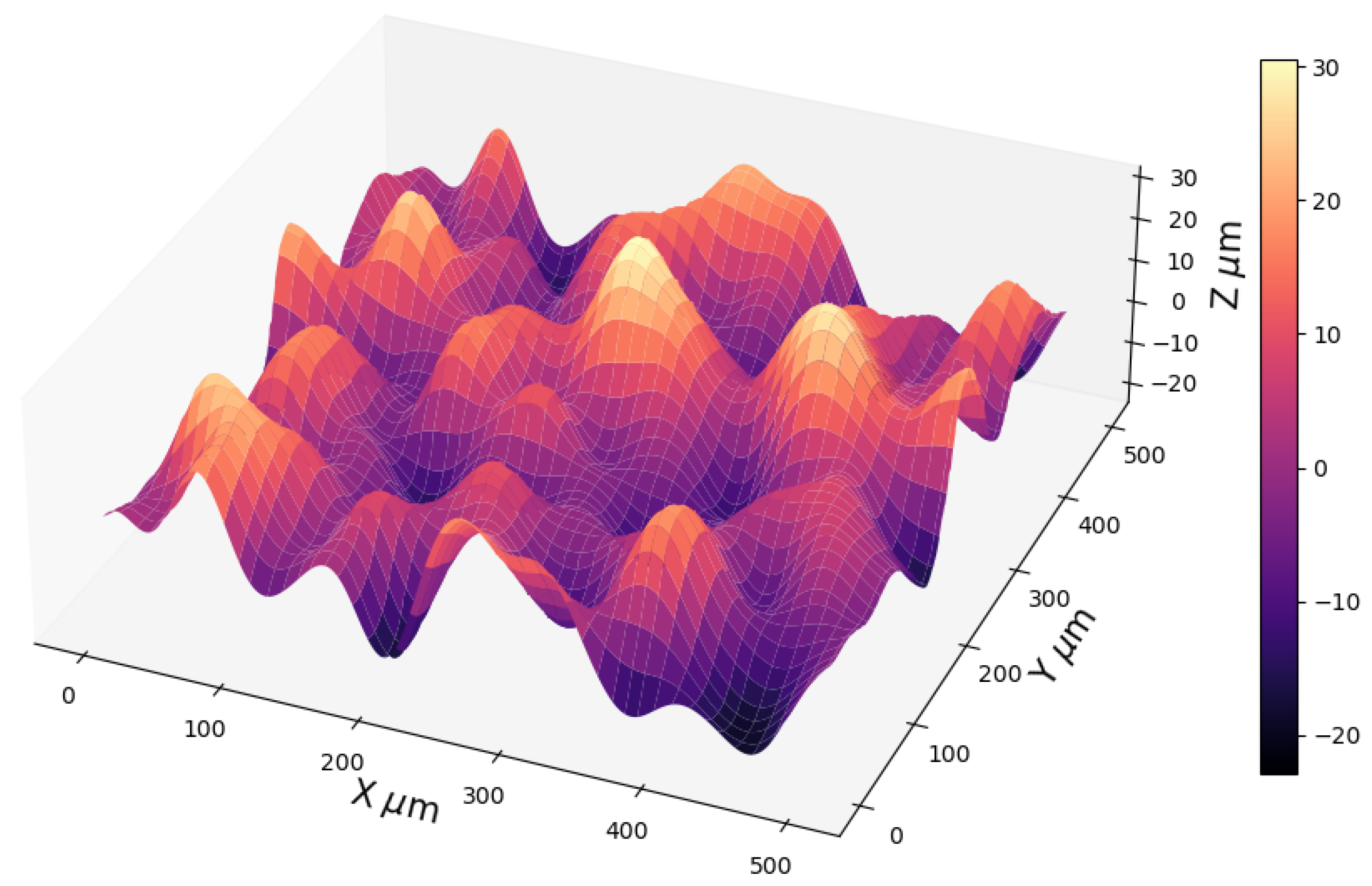
where x, y are the positions of the center of the Gaussian, and are the correlation length for the x, y directions, respectively. The correlation lengths of an autocorrelation function is defined as the value at which the function decays 1/e from its initial value, and it is a measure of distance between two features, such as the peaks of the Gaussian bells in a correlated surface [15]. Figure 1 shows an example of a surface generated with this method.
The Garcia and Stoll method has been employed successfully in several works in which the simulation of a random surface has been required, for example for the study of liquid-mediated adhesion between 3D rough surfaces [16], for the surface roughness evolution of a stressed metallic implant [17], and for studying the particle rebound on rough surfaces [18]. For our work, an initial random surface was generated by using the Garcia and Stoll method [10,14], with a random Gaussian distribution for both the height distribution function and the covariance function, where we assumed the surface to be isotropic, i.e., the correlation length at x is equal to the correlation length at y, in order to be more consistent with a real surface without texture [19,20].
2.2. Deformation of the Surface by Magnetic Particle Movements
Experimental investigations show that surface deformations in MRE can generally be found in cuspid-like shapes separated by valleys [8,21,22], where such deformations are attributed to the chain-like formations taking place in the MRE with or without an external magnetic field. Chains are formed due to the interplay between Zeeman and dipolar interactions, with a trend of the magnetic moments of the particles being oriented along the direction of the applied magnetic field [2,3]. The intensity of the field affects the quantity and size of the chains, thus affecting the surface and therefore the roughness. To simulate these deformations, a system is modeled which consists of an elastic matrix with randomly distributed magnetic particles, and a random roughness profile is incorporated using the methods mentioned above. The movement of the particles is performed by using a standard Monte Carlo method with Metropolis dynamics in the framework of a Hamiltonian containing dipolar and Zeeman interaction terms. We want to stress that during every single Monte Carlo step, trials consist of attempts of new magnetic moment orientations and new random positions displacements for every single particle. Each of these movements generates a change on the surface, having at the end a system in equilibrium with a modified surface. The roadmap in this work is to separate the system into two parts, namely, a first one consisting of a matrix with embedded magnetic particles evolving toward equilibrium, and a second one is the surface itself. This is proposed for the following reasons: (1) computational cost decreases by separating the processes, (2) observation windows of the evolution of the system can be taken and displayed graphically, without the need for using the same equipment for the simulation; that is, the equilibration of the particle movements can be performed on a computer, such as a laptop, different to others where surface reconstruction and visualization can be carried out. In this way, simulation can be partitioned into two different tasks. During this process, files containing the initial and final conditions (positions and magnetic moments) for a given value of the external magnetic field can be generated and stored, and the respective surfaces can be reconstructed.
2.3. Methodology for Surface Deformation
In a first step, an initial random surface is generated by using the Garcia and Stoll model [10,14]. Surface reconstruction depends on the change in the position of the particles in the system and above each particle near the surface, and the appearance of it is modeled by means of a 3D Gaussian bell of the form:
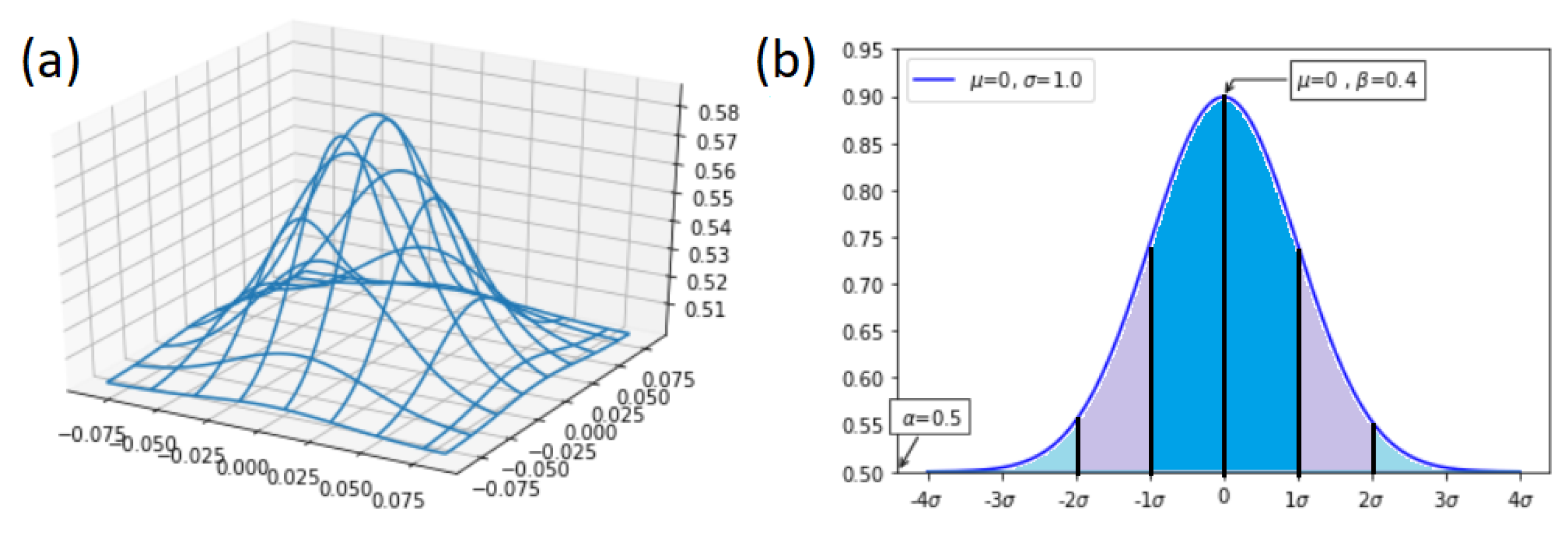
where is the height where the Gaussian bell begins, is the maximum bell height, x, y are the positions of the center of the bell, and is the standard deviation which is the same as the radius of the particle lying below the bell. The bell grows proportional to the change in height, that is, the greater the change in height the larger the size of the bell; therefore, the parameter is dependent on this change, where this is taken as the value of the change in height of the particles. Since the complete graph comprises flattened portions beyond three times the standard deviation, a suitable cut-off was chosen to be among the limits from to as shown in Figure 2, so as not to affect the surface too much. This model allows the creation of peaks and valleys in the z direction, if the displacement of particles is either positive or negative.
The random initial matrix of the surface is a mesh of specific points which are uncorrelated with the positions of the magnetic particles underlying the surface. Since the displacements of the particles (due, for instance, to the applied magnetic field or to the dipolar interaction) will be responsible for the surface deformations, the two layers of points, namely and , must be somehow coupled or concatenated. To do that, a surface interpolation function was defined by using Python’s interp2d function from Scipy library [23], so we can find or add any point within it. The goal with this is to be able to deform the points of the surface mesh with a Gaussian function whose centroid coincides with the closest magnetic particle right below. The magnetic particles that generate the deformation are those closer to the surface, since it is assumed that the innermost particles, away from the surface, will not affect it. Such an assumption was made considering only those particles closest to the surface, within a band of 30% of the total height of the initial simulation box. For percentages higher than this, the value of the percentage of surface deformation varies less, with differences of less than 1%.
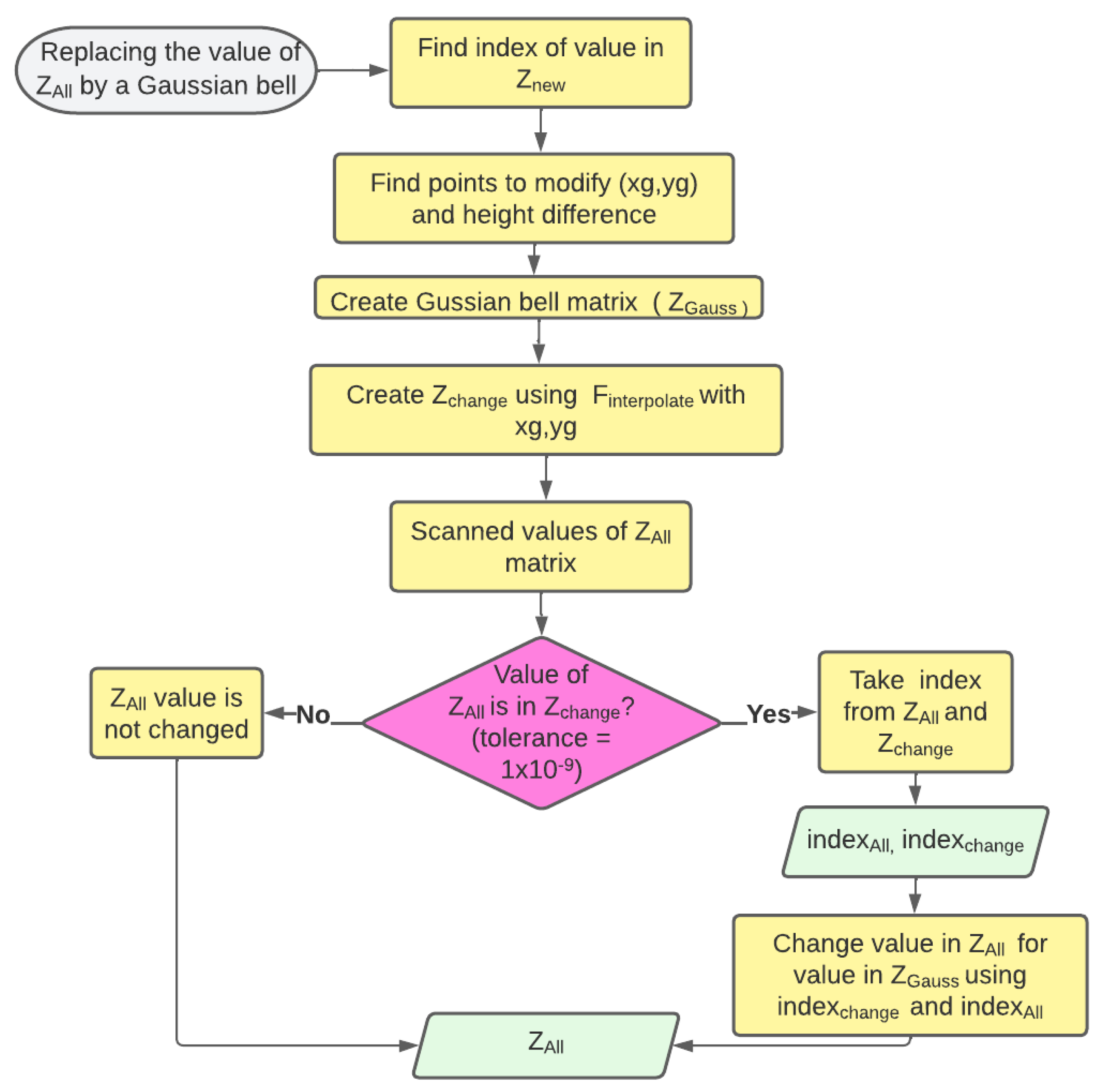
The process to achieve this is as follows: First, the initial mesh positions (x, y) are concatenated with the final positions of the magnetic particles generating all the necessary points to modify the surface. Then, using the interpolation function, two matrices are generated, the matrix using the and positions, which will be the basis for the rest of the algorithm, and the matrix using and positions, with the purpose of identifying these positions in the matrix, to generate the deformation through a Gaussian function. As mentioned above, the displacement of the particles generates the deformation, therefore it is necessary to create an array that contains these values; in this case, the displacements in the z direction are stored. These are calculated as the difference between the initial and final locations of each particle, named as Z, which corresponds in turn to the parameter in Equation (2). This methodology is summarized in Flowchart 1 in Figure 3, showing data processing from the creation of the surface to the modification of it; however, in the binary execution step, where and are compared, it is necessary to deepen its operation. In this step, if the decision is “Yes”, we proceed to the methodology of the replacement of the area affected by the particle movement, as summarized in Flowchart 2 in Figure 4. Taking into account the large number of steps involved in the modeling, Flowchart 1 integrates all the variables and matrices necessary for the creation and subsequent modification of the surface, whereas Flowchart 2 specifies the way in which these variables and matrices will be used to generate the modification in specific regions of the surface, more concretely, those local zones influenced by the presence of particles underlying the surface. To achieve this, we proceed as follows:
- 1.
- Indices formed by pairs of integers (row, column) in the 2D data matrix are identified for easy access of the real value points (,).
- 2.
- The surface points to be affected by the Gaussian bell are determined within a cut-off region (,).
- 3.
- The matrix containing the Gaussian bell () is created using the points from step 2.
- 4.
- A matrix is created using the interpolation function ().
- 5.
- The complete surface matrix () is scanned to be modified.
- 6.
- If the value scanned of matches with any value of with a tolerance of 1 × 10⁻⁹, it is modified with the value found in . If the value does not match, it is not modified.
In step 1, the real value of the z coordinate linked to every index value in the matrix corresponds to the parameter in Equation (2). Such a value represents the baseline above which the Gaussian bell is built.
In step 2, the extension of the region to be modified is identified using the particle radius ( in Equation (2)), whereas the (,) coordinates determine the center of the Gaussian bell. At this step, a new array of points (,) is needed to build the Gaussian bell, whose values range from the central position of the particle (,) to the cut-off values described above.
Step 3 creates the matrix containing all the height values covering the Gaussian bell surface.
Step 4 creates a fourth matrix () using the interpolation function and the positions to be modified (,). This matrix acts as a bridge between the matrix of the whole surface and the section to be modified with .
In step 5, the matrix of the entire surface is scanned to be modified using the next step. Thus, in step 6, is modified with if the tolerance of the comparison between and is fulfilled, otherwise the surface remains the same.
Particles were treated as single-domain particles interacting each other via dipolar interactions and with a uniform external applied magnetic field along the z-direction through a Zeeman interaction. Simulation was performed over 243 magnetite particles of 0.8 μm radius, inside a box of 30 × 30 × 10 μm3, this is shown in Figure 5.
3. Results and Discussion
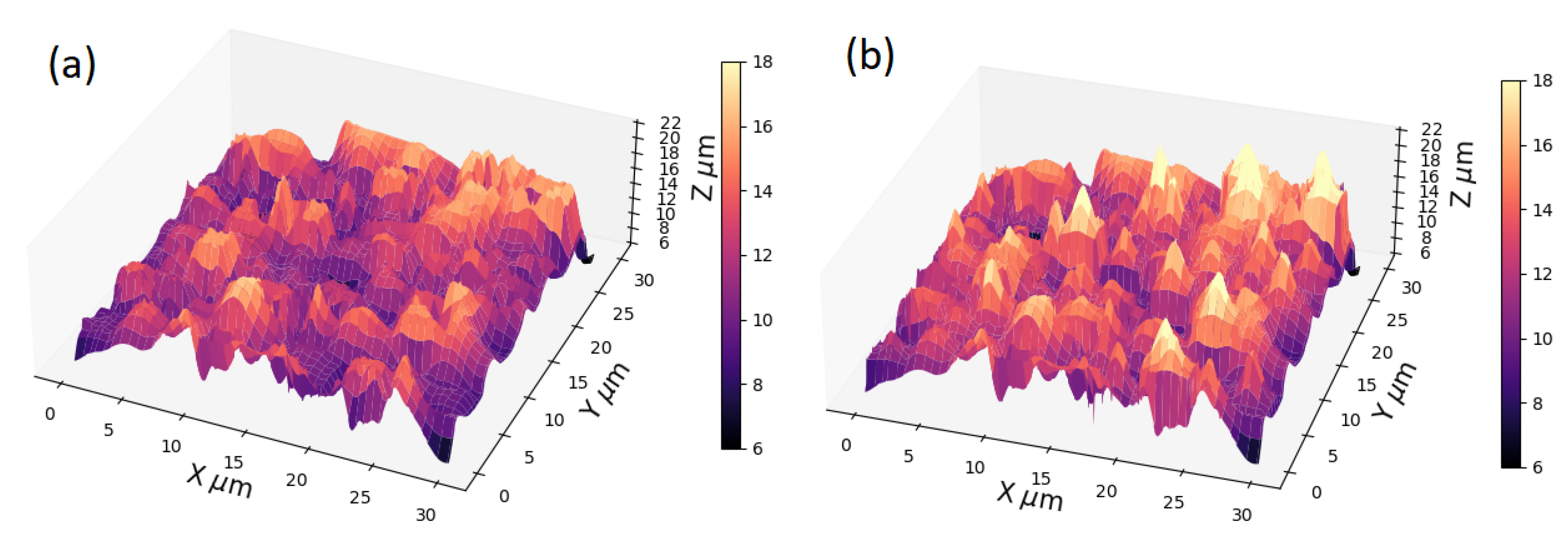
Two random surfaces were considered. One involved a higher correlation length ( = = 2 μm, isotropic surface) in order to obtain a smoother surface as shown in Figure 6. A second surface with a lower correlation length ( = = 0.4 μm, isotropic surface), which makes the surface noisier, was also simulated. This last one, however, allows us to identify on the surface those regions below which the particles are located. The RMS height values were both 2 μm. Surface deformations were performed using the methodology described in the previous section, using 400 points for the initial grid, which subsequently increases in size due to the particles, obtaining a final grid of 463 points. The results of test 1 are shown in Figure 6, the results of test 2 are shown in Figure 7 and Figure 8. The calculation of the RMS roughness parameter was performed using the following expression (standard deviation of heights) [24]:
where N is the total number of points on the surface (total points after deformation, for both tests), is the height at each point on the surface, and is the average of the heights.
We can observe that the surface has been modified in several sections due to the conglomerate of magnetic particles. Such deformations are consistent with a topography of valleys and peaks as observed in experimental work [7,21,22].
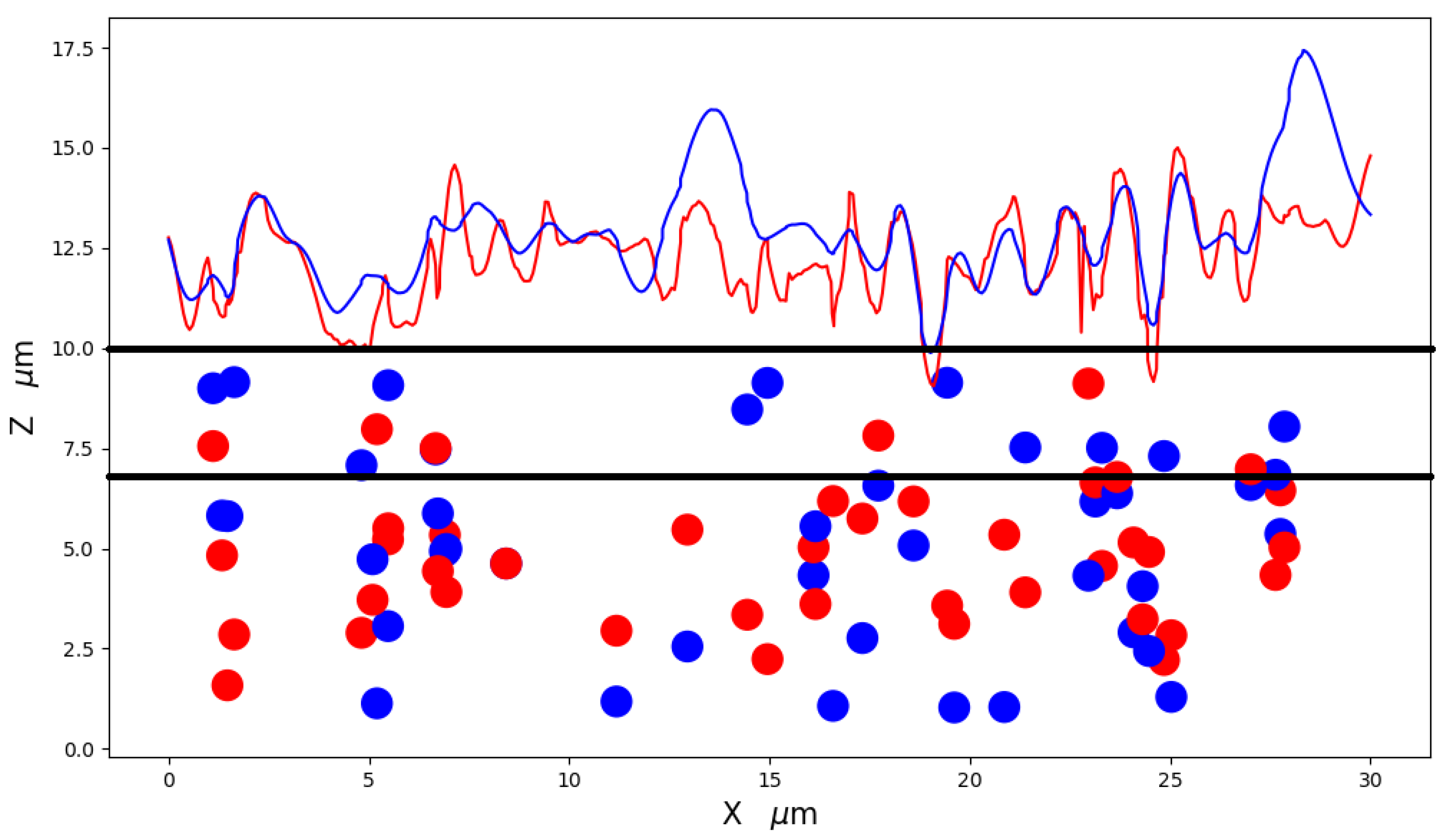
In Figure 7, we can observe the output surface deformation arising from the particle displacement, which is more noticeable for test 2, finding that the valleys and peaks formation is clearer and more differentiated than the initial surface. In order to better visualize this deformation, Figure 8 shows a cross section at y = 15 m where the deformation, due to several particles found in these coordinates, is observed. As the particles move, the region consistent with their sizes becomes accordingly modified. This process was carried out using two system files keeping the same input parameters, e.g., particle size, number of particles, external magnetic field, and size of the simulation box. The change between the two systems lies in the initial positions of the particles, in order to obtain two comparable deformations. We found that the deformation percentages of both systems are practically the same. For instance, by using the parameters of test 1 (Table 1) for two different initial systems, the deformation percentage for system 1 was , whereas for system 2 it was .
The values of roughness and percentages of deformation for four tests, each one consisting of two replicas are summarized in Table 1.
The deformation percentage tells us how much the surface has changed. Results demonstrate that larger percentages of deformation are obtained in test 2, corresponding to the case where the particle size is greater than the correlation length. We want to stress that up to five different simulations were performed in every case for different seeds of the random number generator used.
4. Conclusions
It was possible to develop a numerical methodology capable of modifying the surface of an elastomer-particle magnetorheological system by considering the respective coordinates and sizes of the embedded magnetic particles. The method employed matrix arrays for the creation and modification of the surfaces, and, as such, modifications in specific regions of the surface, i.e., those local zones influenced by the presence of particles underlying the surface, can be undertaken.
The main two differences to highlight with respect to other works in the literature related to the simulation and reconstruction of rough surfaces are:
- Our method allows us to obtain a mathematical function that is fed by a grid of points (x, y) in order to reproduce a modified and equilibrated surface, which can be then exported for later use (for instance, to analyze the interaction of a rough surface with a drop of water for obtaining contact angles) by means of an output file.
- Our method considers the internal structure of the elastomer to a certain depth in 3D, in such a way that the presence of particles embedded and their influence, within a range, upon the surface roughness, was tackled.
The main limitation deals with the fact that the elastomer matrix in our model is considered as a continuous medium where, in fact, its own microscopic structure based on chains of molecules and textures is also an ingredient affecting the roughness of the surface. In this sense, future work should also take into account these details, as well as the elastic coupling of the particles to the elastomer matrix.
Verification with experimental results is currently in progress in our group, where we are synthesizing PDMS elastomers with magnetite nanoparticles and performing surface analysis with atomic force microscopy techniques. The idea behind this type of synthesis is to obtain a material where it is possible to modify the roughness with the application of a magnetic field.
We are confident that this approach can help in the understanding of the morphology and surface properties of MRE systems.
Author Contributions
Conceptualization, J.A.V., H.D.S., J.R., and E.R.; methodology, J.A.V.; software, J.A.V.; validation, J.A.V. and H.D.S.; formal analysis, J.A.V. and H.D.S.; investigation, J.A.V.; data curation, H.D.S.; writing—original draft preparation, J.A.V.; writing—review and editing, J.R., E.R.; visualization, J.A.V.; supervision, J.R. and E.R.; funding acquisition, J.R. and E.R. All authors have read and agreed to the published version of the manuscript.
Funding
J.R. acknowledges the Universidad de Antioquia, E.R. acknowledges the Universidad Nacional de Colombia, for the exclusive dedication program. Financial support was provided by Minciencias under the program “Desarrollo de un sistema para la remoción de contaminantes en agua usando nano partículas obtenidas con reactores de membrana” code 111985270600, Universidad Nacional de Colombia and Universidad de Antioquia.
Institutional Review Board Statement
Not applicable.
Data Availability Statement
Data presented in this study are available in GitHub.
Conflicts of Interest
The authors declare no conflict of interest.
Abbreviations
Given the large number of variables and abbreviations used in this work, this section summarizes the name and simple meaning each one of them.
| MRE | Magnetorheological elastomer. |
| hdf | Height distribution function. |
| acf | Autocovariance function. |
| and | correlation length for the x,y direction respectively. |
| Height value where the Gaussian bell begins. | |
| Maximum Gaussian bell height. | |
| Standard deviation. | |
| Random initial matrix, using the Garcia and Stoll method. | |
| Mesh points of . | |
| Positions of the magnetic particles. | |
| Surface interpolation function, using to interpolate . | |
| Final positions of the magnetic particles. | |
| Positions resulted of a concatenate initial mesh positions with final | |
| positions of magnetic particles. | |
| Surface matrix generated by using with . | |
| Surface matrix generated by using with . | |
| Z | Difference between the initial and final locations of each particle. |
| ,. | Array of points whose values range from the central position of the |
| particle to the cut-off. | |
| Matrix containing the Gaussian bell with , positions. | |
| Matrix of the points to affected by Gaussian bell using | |
| with ,. | |
| Root mean square roughness (RMS roughness). |
References
- Liu, T.; Xu, Y. Magnetorheological Elastomers: Materials and Applications. Smart Funct. Soft Mater. 2019. [Google Scholar] [CrossRef] [Green Version]
- Glavan, G.; Salamon, P.; Belyaeva, I.A.; Shamonin, M.; Drevenšek-Olenik, I. Tunable surface roughness and wettability of a soft magnetoactive elastomer. J. Appl. Polym. Sci. 2018, 135, 46221. [Google Scholar] [CrossRef]
- Danas, K.; Kankanala, S.V.; Triantafyllidis, N. Experiments and modeling of iron-particle-filled magnetorheological elastomers. J. Mech. Phys. Solids 2012, 60, 120–138. [Google Scholar] [CrossRef]
- Sánchez, P.A.; Minina, E.S.; Kantorovich, S.S.; Kramarenko, E.Y. Surface relief of magnetoactive elastomeric films in a homogeneous magnetic field: Molecular dynamics simulations. Soft Matter 2019, 15, 175–189. [Google Scholar] [CrossRef] [Green Version]
- Gervasio, M.; Lu, K. Monte Carlo Simulation Modeling of Nanoparticle-Polymer Cosuspensions. Langmuir 2019, 35, 161–170. [Google Scholar] [CrossRef] [PubMed]
- Nadzharyan, T.A.; Shamonin, M.; Kramarenko, E.Y. Theoretical Modeling of Magnetoactive Elastomers on Different Scales: A State-of-the-Art Review. Polymers 2022, 14, 4096. [Google Scholar] [CrossRef]
- Li, R.; Li, X.; Li, Y.; Yang, P.A.; Liu, J. Experimental and numerical study on surface roughness of magnetorheological elastomer for controllable friction. Friction 2020, 8, 917–929. [Google Scholar] [CrossRef] [Green Version]
- Li, R.; Li, X.; Yang, P.A.; Liu, J.; Chen, S. The field-dependent surface roughness of magnetorheological elastomer: Numerical simulation and experimental verification. Smart Mater. Struct. 2019, 28, 085018. [Google Scholar] [CrossRef]
- Chen, S.; Li, R.; Li, X.; Wang, X. Magnetic field induced surface micro-deformation of magnetorheological elastomers for roughness control. Front. Mater. 2018, 5, 76. [Google Scholar] [CrossRef]
- Garcia, N.; Stoll, E. Monte Carlo Calculation for Electromagnetic-Wave Scattering from Random Rough Surfaces. Phys. Rev. Lett. 1984, 52, 1798. [Google Scholar] [CrossRef]
- Shiwei, C.; Shuai, D.; Xiaojie, W.; Weihua, L. Magneto-induced surface morphologies in magnetorheological elastomer films: An analytical study. Smart Mater. Struct. 2019, 28, 045016. [Google Scholar] [CrossRef]
- Mack, C.A. Generating random rough edges, surfaces, and volumes. Appl. Opt. 2013, 52, 1472–1480. [Google Scholar] [CrossRef] [PubMed] [Green Version]
- Naylor, T. Computer Simulation Techniques; John Wiley & Sons Inc.: Hoboken, NJ, USA, 1966. [Google Scholar]
- Bergström, D.; Powell, J.; Kaplan, A.F.H. The absorption of light by rough metal surfaces-A three-dimensional ray-tracing analysis. Citation J. Appl. Phys. 2008, 103, 113504. [Google Scholar] [CrossRef]
- Taconet, O.; Ciarletti, V. Estimating soil roughness indices on a ridge-and-furrow surface using stereo photogrammetry. Soil Tillage Res. 2007, 93, 64–76. [Google Scholar] [CrossRef]
- Rostami, A.; Streator, J.L. Study of liquid-mediated adhesion between 3D rough surfaces: A spectral approach. Tribol. Int. 2015, 84, 36–47. [Google Scholar] [CrossRef]
- Tan, H. In vivo surface roughness evolution of a stressed metallic implant. J. Mech. Phys. Solids 2016, 95, 430–440. [Google Scholar] [CrossRef]
- Altmeppen, J.; Sommerfeld, H.; Koch, C.; Staudacher, S. An analytical approach to estimate the effect of surface roughness on particle rebound. J. Glob. Power Propuls. Soc. 2020, 4, 27–37. [Google Scholar] [CrossRef]
- Damiati, L.; Eales, M.G.; Nobbs, A.H.; Su, B.; Tsimbouri, P.M.; Salmeron-Sanchez, M.; Dalby, M.J. Impact of surface topography and coating on osteogenesis and bacterial attachment on titanium implants. J. Tissue Eng. 2018, 9, 2041731418790694. [Google Scholar] [CrossRef] [PubMed]
- Trevisani, S.; Cavalli, M. Topography-based flow-directional roughness: Potential and challenges. Earth Surf. Dyn. 2016, 4, 343–358. [Google Scholar] [CrossRef] [Green Version]
- Johari, M.A.F.; Mazlan, S.A.; Nasef, M.M.; Ubaidillah, U.; Nordin, N.A.; Aziz, S.A.A.; Johari, N.; Nazmi, N. Microstructural behavior of magnetorheological elastomer undergoing durability evaluation by stress relaxation. Sci. Rep. 2021, 11, 10936. [Google Scholar] [CrossRef] [PubMed]
- Iacobescu, G.E.; Balasoiu, M.; Bica, I. Investigation of surface properties of magnetorheological elastomers by atomic force microscopy. J. Supercond. Nov. Magn. 2013, 26, 785–792. [Google Scholar] [CrossRef]
- Python scipy.interpolate.interp2d—SciPy v1.8.0 Manual. Available online: https://docs.scipy.org/doc/scipy/reference/generated/scipy.interpolate.interp2d.html (accessed on 7 November 2022).
- Oliveira, R.D.; Albuquerque, D.; Cruz, T.; Yamaji, F.; Leite, F.; Oliveira, R.D.; Albuquerque, D.; Cruz, T.; Yamaji, F.; Leite, F. Measurement of the Nanoscale Roughness by Atomic Force Microscopy: Basic Principles and Applications. In Atomic Force Microscopy—Imaging, Measuring and Manipulating Surfaces at the Atomic Scale; IntechOpen: London, UK, 2012. [Google Scholar] [CrossRef] [Green Version]
Figure 1.
Three-dimensional random surface with RMS height of 5 m, = 40 m, and = 50 m.

Figure 2.
Gaussian bell cut from to : (a) 3D Gaussian bell, (b) a typical 2D section of the 3D Gaussian bell.
Figure 2.
Gaussian bell cut from to : (a) 3D Gaussian bell, (b) a typical 2D section of the 3D Gaussian bell.

Figure 3.
Flowchart 1, complete cycle of the deformation of a random surface.

Figure 4.
Flowchart 2, change of surface values using the and matrices.

Figure 5.
Three-dimensional elastomer-magnetic particle system, the color is associated with the z-component of spin. (a) System before applying magnetic field. (b) System after applying magnetic field.
Figure 5.
Three-dimensional elastomer-magnetic particle system, the color is associated with the z-component of spin. (a) System before applying magnetic field. (b) System after applying magnetic field.

Figure 6.
Three-dimensional surface for the elastomer-magnetic particle system for test 1 with RMS height of m, = m, and = m (a) Initial surface without modification. (b) Surface modified by the movement of the particles.
Figure 6.
Three-dimensional surface for the elastomer-magnetic particle system for test 1 with RMS height of m, = m, and = m (a) Initial surface without modification. (b) Surface modified by the movement of the particles.

Figure 7.
Three-dimensional surface for the elastomer-magnetic particle system for test 2 with RMS height of 2 m, = 0.4 m, and = 0.4 m (a) Initial surface without modification. (b) Surface modified by the movement of the particles.
Figure 7.
Three-dimensional surface for the elastomer-magnetic particle system for test 2 with RMS height of 2 m, = 0.4 m, and = 0.4 m (a) Initial surface without modification. (b) Surface modified by the movement of the particles.

Figure 8.
Cross section of the 3D surface for test 2 comparison of initial profile (red line) and modified profile (blue line). Parallel horizontal black lines represent the band of 30% of the total height of the initial simulation box.
Figure 8.
Cross section of the 3D surface for test 2 comparison of initial profile (red line) and modified profile (blue line). Parallel horizontal black lines represent the band of 30% of the total height of the initial simulation box.


Table 1.
Results for 4 tests with their respective initial values, (SC: surface created, MS: modified surface).
Table 1.
Results for 4 tests with their respective initial values, (SC: surface created, MS: modified surface).
| Test | RMS Input | RMS SC | RMS MS | % Deformation | ||
|---|---|---|---|---|---|---|
| 1 | 2 m | 2 m | 2 m | 2.1 m | 2.4 m | |
| 2 | 2 m | 0.4 m | 0.4 m | 1.7 m | 2.2 m | |
| 3 | 1 m | 2.2 m | 2.2 m | 1.1 m | 1.6 m | |
| 4 | 1.5 m | 0.3 m | 0.3 m | 1.2 m | 1.9 m |
Disclaimer/Publisher’s Note: The statements, opinions and data contained in all publications are solely those of the individual author(s) and contributor(s) and not of MDPI and/or the editor(s). MDPI and/or the editor(s) disclaim responsibility for any injury to people or property resulting from any ideas, methods, instructions or products referred to in the content. |
© 2023 by the authors. Licensee MDPI, Basel, Switzerland. This article is an open access article distributed under the terms and conditions of the Creative Commons Attribution (CC BY) license (https://creativecommons.org/licenses/by/4.0/).
Share and Cite
MDPI and ACS Style
Valencia, J.A.; Restrepo, J.; Salinas, H.D.; Restrepo, E. Numerical Study on Surface Reconstruction and Roughness of Magnetorheological Elastomers. Computation 2023, 11, 46. https://doi.org/10.3390/computation11030046
AMA Style
Valencia JA, Restrepo J, Salinas HD, Restrepo E. Numerical Study on Surface Reconstruction and Roughness of Magnetorheological Elastomers. Computation. 2023; 11(3):46. https://doi.org/10.3390/computation11030046
Chicago/Turabian StyleValencia, José Antonio, Johans Restrepo, Hernán David Salinas, and Elisabeth Restrepo. 2023. "Numerical Study on Surface Reconstruction and Roughness of Magnetorheological Elastomers" Computation 11, no. 3: 46. https://doi.org/10.3390/computation11030046
Note that from the first issue of 2016, this journal uses article numbers instead of page numbers. See further details here.