On Fitting the Lomax Distribution: A Comparison between Minimum Distance Estimators and Other Estimation Techniques

Abstract

In this paper, we investigate the performance of a variety of frequentist estimation techniques for the scale and shape parameters of the Lomax distribution. These methods include traditional methods such as the maximum likelihood estimator and the method of moments estimator. A version of the maximum likelihood estimator adjusted for bias is included as well. Furthermore, an alternative moment-based estimation technique, the L-moment estimator, is included, along with three different minimum distance estimators. The finite sample performances of each of these estimators are compared in an extensive Monte Carlo study. We find that no single estimator outperforms its competitors uniformly. We recommend one of the minimum distance estimators for use with smaller samples, while a bias-reduced version of maximum likelihood estimation is recommended for use with larger samples. In addition, the desirable asymptotic properties of traditional maximum likelihood estimators make them appealing for larger samples. We include a practical application demonstrating the use of the described techniques on observed data.

1. Introduction

The Pareto distribution is a heavy-tailed distribution that was originally developed in the 19th century to model the distribution of income among individuals [1]. However, in the years following its introduction it has been extensively modified and changed to produce several variants, referred to as the Type I, II, III, and IV Pareto distributions, as well as the so-called generalised Pareto distribution (GPD). The focus of this paper is on the Pareto Type II distribution, in which the location parameter is zero, which is known as the Lomax distribution. This rather popular distribution was originally introduced to model business failure data [2], and has subsequently been employed as a model in a wide range of settings. This distribution has proven useful in modelling survival times when censoring is present, e.g., in the lifetimes of electric power transformers [3]; as the times are left-truncated and right-censored, when they are modelled it is found that the Lomax distribution provides the best fit among the various distributions considered. As another example, the exponential Lomax and Weibull Lomax are a good fit for right-censored lung cancer survival data [4].

Other scenarios in which the Lomax distribution has been used as a model include wealth distribution [5], the distribution of queueing service times [6], life testing [7], and the sizes of files on a computer server [8], to name only a few.

We can say that a random variable X follows a Lomax distribution with scale parameter $\sigma >0$ and shape parameter $\beta >0$ if its cumulative distribution function (CDF) is

$$F_{\sigma ,\beta }\left(x\right)=1-{\left[1+\left(\frac{x}{\sigma }\right)\right]}^{-\beta },x>0,$$

with a probability density function (PDF) of

$$f_{\sigma ,\beta }\left(x\right)=\frac{\beta }{\sigma }{\left(1+\frac{x}{\sigma }\right)}^{-(\beta +1)},x>0.$$

In this paper, we investigate different approaches used for estimating the parameters of the Lomax distribution. We draw parallels with the methods used to estimate the parameters of other distributions in order to ascertain how one might go about obtaining reliable estimators. For example, when considering the estimation of the parameters of the GPD, a number of approaches have been studied, such as maximum likelihood estimation (MLE), method of moment estimation (MME), L-moment estimation (LME), and probability-weighted moment estimation (PWME). However, not all approaches are equally viable in all settings. It was noted in [9], for example, that MLE experiences difficulty when estimating the parameters of the GPD under a variety of configurations of the shape and scale parameter values. Similarly, ref. [10] found that the usefulness of MLE is restricted to very large sample sizes; instead, the use of PWME is advocated in case of moderate sample sizes. Several studies similar to the one presented in this paper have been conducted for other distributions; to mention only a few examples, ref. [11] considered improved estimators for the generalised gamma distribution using small samples, whereas [12,13] compared a variety of different estimators for the parameters of the unit-gamma and Weibull distributions, respectively. For the Lomax distribution in particular, studies include [14,15]. These papers are concerned with the estimation of Lomax parameters using diverse traditional methods of estimation, including MLE, MME, and PWME. The results of these methods have been compared to one another and recommendations have been made concerning the use of these more traditional estimation approaches. From previous papers, it is clear that MLE approaches are not particularly reliable when used with moderately large samples. The conclusion from these studies is that though traditional approaches have utility in certain settings, none are generally applicable.

The aim of this paper is twofold. First, we provide an overview of estimation techniques used for the Lomax distribution and compare the performance of various estimators. Second, we focus on the minimum distance estimators (MDEs), which represent an unexplored avenue for estimating the parameters of the Lomax distribution. While a number of these procedures have already been examined in [16] for the GPD, focusing on the Lomax distribution can provide specific insight into the usefulness of these methods for this particular distribution. In addition, the MDEs we consider here differ substantially from those proposed in [16,17] in that their paper only considered density power divergence measures, whereas we additionally explore distribution function-based methods.

Generally speaking, MDEs measure the difference between an empirical estimate of the probability density or distribution function and the theoretical function [18]. The use of minimum distance estimation measures has been advocated by a number of authors, including [19,20,21], when modelling data containing extreme values, as these estimators have good robustness qualities.

This paper studies the general case in which both the scale ($\sigma$) and shape ($\beta$) parameters of the Lomax distribution are unknown. We start by considering the myriad different traditional estimation methods proposed for related distributions, including the L-moment estimator, the MLE, and the MME. We then proceed to propose the use of MDEs in the hope that these may represent competitive alternatives to the more traditional estimators. Although we do not consider any Bayesian estimators in this study, we refer interested readers to [22] and the very recent paper by [23], where Bayesian estimators for the Lomax distribution are discussed and compared, as well as to [24], where Bayesian estimation of the two-parameter gamma distribution is discussed. The performance of the estimators are compared to one another through a comprehensive numerical study involving Monte Carlo simulations in which the finite sample variance, relative bias, and mean squared error (MSE) of each estimator are approximated. In addition, an omnibus measure allowing the MSE of the estimation of both $\sigma$ and $\beta$ to be gauged simultaneously is employed in the simulation study.

The remainder of this article is organised as follows. In Section 2, the different parameter estimation methods are introduced and discussed. Next, the Monte Carlo study is presented in Section 3, including a detailed discussion of the simulation results. In Section 4, we apply the different estimators to a real world example. Finally, in Section 5, we conclude the paper by making a number of general observations regarding the estimators and provide recommendations concerning their use.

2. Estimation of Parameters

In this section, we discuss the parameter estimation methods used to estimate the shape and scale parameters of the Lomax distribution. Included here are traditional methods of parameter estimation as well as methods based on optimising a variety of distance measures. In addition to the performance of the MDEs, we provide an overview of the performance of a wide variety of competing estimators. This facilitates recommendations regarding the choice of estimator to be used in various settings. Theoretical details relevant to the estimation of the parameters are provided in each case.

For the remainder of the section, we assume that we have data $X_1,X_2,\dots ,X_n$ which are independently and identically distributed (i.i.d.) from the Lomax distribution with parameters $\beta >0$ and $\sigma >0$. The order statistics based on this sample are denoted using $X_{1:n}\le X_{2:n}\le \cdots \le X_{n:n}$.

2.1. Method of Moment Estimators (MMES)

MME is one of the most widely used estimation techniques. It has been used to investigate key aspects of probability distributions, such as central tendency, spread, skewness, and kurtosis. However, for the Lomax distribution, due to the fact that with shape parameter $\beta$ only moments lower than $\beta$ are finite, this approach is often not ideal for the parameters of the Lomax distribution. It is ultimately presented here and in the Monte Carlo in Section 3.1 in order to illustrate its functionality for a range of values of $\beta$.

To derive the MMEs for the Lomax distribution, we can note that the $r^{\mathrm{th}}$ theoretical raw moment of the distribution is

$$\mathrm{E}\left(X^r\right)={\mu }_r=\frac{{\sigma }^r\Gamma (\beta -r)\Gamma (1+r)}{\Gamma \left(\beta \right)},0<r<\beta r=1,2,\cdots .$$

The first and second theoretical raw moments are then provided by

$$\mathrm{E}\left(X\right)={\mu }_1=\frac{\sigma }{\beta -1},\mathrm{and}\mathrm{E}\left(X^2\right)={\mu }_2=\frac{2{\sigma }^2}{(\beta -1)(\beta -2)}.$$

(1)

From (1), we can express $\beta$ and $\sigma$ as

$$\beta =\frac{2{\mu }_2-2{\mu }_1^2}{{\mu }_2-2{\mu }_1^2}\mathrm{and}\sigma ={\mu }_1(\beta -1).$$

(2)

By simply substituting ${\mu }_1$ and ${\mu }_2$ with their sample estimators in (2), the MMEs of these parameters are obtained:

$${\widehat{\beta }}_{MM}=\frac{2{\widehat{\mu }}_2-2{\widehat{\mu }}_1^2}{{\widehat{\mu }}_2-2{\widehat{\mu }}_1^2}\mathrm{and}{\widehat{\sigma }}_{MM}={\widehat{\mu }}_1({\widehat{\beta }}_{MM}-1),$$

where ${\widehat{\mu }}_r=\frac{1}{n}{\sum }_{i=1}^n{X}_i^r,r=1,2$.

2.2. L-Moment Estimators (LMEs)

L-moments provide an alternative way to describe the shapes of probability distributions, and are defined as the expected values of linear combinations of order statistics. They were proposed in [25] as robust alternatives to classical moments. The method of L-moments has advantages over classical moments, including unbiasedness, robustness to the presence of outliers in the data, and lower sensitivity to sampling variability, especially when the data of interest are heavy-tailed, as is the case in our context. If the mean of the distribution exists, it follows that all of the L-moments exist and uniquely define the distribution [25]. The $r^{\mathrm{th}}$ population L-moment is provided by

$${\lambda }_r=\frac{1}{r}\sum _{k=0}^{r-1}{(-1)}^k\left(\genfrac{}{}{0pt}{}{r-1}{k}\right)\mathrm{E}\left(X_{r-k:r}\right),r=1,2,\cdots ,$$

where r is the integer order of the L-moment and $\mathrm{E}\left(X_{r-k:r}\right)$ is the expectation of the ${(r-k)}^{\mathrm{th}}$ order statistic of a sample of size r. The sample L-moment is provided by

$$l_r={\left(\genfrac{}{}{0pt}{}{n}{r}\right)}^{-1}\underset{1\le i_1<\dots <i_r\le n}{\sum \sum \cdots \sum }\frac{1}{r}\sum _{k=0}^{r-1}{(-1)}^k\left(\genfrac{}{}{0pt}{}{r-1}{k}\right)X_{i_{r-k}:n}r=1,2,\cdots ,n.$$

Therefore, the expressions of the first two sample L-moments are

$$l_1=\frac{1}{n}\sum _{i=1}^n{X}_{i:n}=\overline{X}\mathrm{and}{l}_2=\frac{1}{2}{\left(\genfrac{}{}{0pt}{}{n}{2}\right)}^{-1}\underset{i>j}{\sum \sum }(X_{i:n}-X_{j:n}),$$

where $\overline{X}$ is the sample mean.

Similar to the method of moments, the L-moments can be used to obtain parameter estimates by equating the theoretical L-moments of the distribution to the corresponding L-moments of a sample. Therefore, the L-moment estimators of the parameters of the Lomax distribution are provided by

$${\widehat{\beta }}_{LM}=\frac{l_2}{2l_2-l_1}\mathrm{and}{\widehat{\sigma }}_{LM}=\frac{l_1^2-l_1{l}_2}{2l_2-l_1};$$

see [15]. L-moments can be a good starting point for the iterative numerical procedure needed to obtain maximum likelihood estimates [26].

Remark 1.

Note that the probability-weighted moment estimators (PWMEs) proposed in [27] were considered for this paper as well; however, they were omitted because they turn out to simply be linear combinations of the LMEs [25,28].

2.3. Maximum Likelihood Estimators (MLEs)

Maximum likelihood estimation is one of the most popular methods for estimating the unknown parameters of probability distributions. The popularity of MLE can be attributable to its desirable asymptotic properties, such as unbiasedness and consistency. However, for small sample sizes, these properties may not hold true, resulting in biased MLEs.

In this section, we first use the MLEs to estimate the unknown parameters; then, in the section that follows, we consider a bias-adjusted approach which reduces the bias of the MLEs to order $O\left(n^{-1}\right)$; see [14].

2.3.1. MLE of the Lomax Distribution

The MLEs for the Lomax distribution are obtained by maximising the log-likelihood function:

$$\ell :=\ell (\beta ,\sigma ;X_1,\dots ,X_n)=nlog\left(\beta \right)-nlog\left(\sigma \right)-(1+\beta )\sum _{i=1}^{n}log\left(1+\frac{X_i}{\sigma }\right).$$

(3)

Differentiating the log-likelihood with respect to $\beta$ and $\sigma$, respectively, yields the equations

$$\frac{\partial \ell }{\partial \beta }=\frac{n}{\beta }-\sum _{i=1}^{n}log\left(1+\frac{X_i}{\sigma }\right),$$

(4)

$$\frac{\partial \ell }{\partial \sigma }=-\frac{n}{\sigma }+\frac{1+\beta }{\sigma }\sum _{i=1}^n\frac{X_i}{\sigma +X_i}.$$

(5)

Unfortunately, we cannot obtain closed-form solutions for both estimators using (4) and (5); thus, numerical procedures are required for optimisation purposes. To simplify the optimisation problem, the expressions can be reduced to the optimisation of a single parameter using the concentrated likelihood estimation approach (the approach followed in [29] using their flomax function). This is accomplished by first noting that when setting (4) to zero and solving, we obtain the MLE ${\widehat{\beta }}_{ML}$ expressed in terms of ${\widehat{\sigma }}_{ML}$:

$${\widehat{\beta }}_{ML}=\frac{n}{{\sum }_{i=1}^{n}log\left(1+X_i/{\widehat{\sigma }}_{ML}\right)}.$$

(6)

The maximised log-likelihood $\widehat{\ell }:=\ell ({\widehat{\beta }}_{ML},{\widehat{\sigma }}_{ML};X_1,\dots ,X_n)$ can therefore be expressed solely in terms of the MLE ${\widehat{\sigma }}_{ML}$ by substituting the form of ${\widehat{\beta }}_{ML}$ provided in (6) and ${\widehat{\sigma }}_{ML}$ into (3):

$$\begin{array}{cc}\hfill \widehat{\ell }& =-nlog\left(\frac{1}{n}\sum _{i=1}^{n}log\left(1+\frac{X_i}{{\widehat{\sigma }}_{ML}}\right)\right)-nlog\left({\widehat{\sigma }}_{ML}\right)-n\left(\frac{1}{n}\sum _{i=1}^{n}log\left(1+\frac{X_i}{{\widehat{\sigma }}_{ML}}\right)+1\right).\hfill \end{array}$$

Then, using R’s one-dimensional optimize [30] function, the MLEs ${\widehat{\sigma }}_{ML}$ and ${\widehat{\beta }}_{ML}$ (via (6)) are obtained.

2.3.2. MLEs of the Lomax Distribution Adjusted for Bias (MLE.b)

For small sample sizes, the MLEs sometimes perform poorly. In order to solve this problem, [14] proposed the use of second-order bias-adjusted versions of the MLEs. To obtain these estimators, the bias of the MLE is first approximated and then subtracted from the MLE to produce the bias-corrected estimate.

Let K be the Fisher information matrix for the Lomax distribution, as provided in [14]. Furthermore, it can be shown that

$$K^{-1}=\left[\begin{array}{cc}\frac{{\sigma }^2}{n\beta }(\beta +2){(\beta +1)}^2& \frac{\sigma \beta }{n}(\beta +1)(\beta +2)\\ \frac{\sigma \beta }{n}(\beta +1)(\beta +2)& \frac{{\beta }^2}{n}{(\beta +1)}^2\end{array}\right].$$

The $O\left(n^{-1}\right)$ bias is obtained in [14] as

$$Bias\left(\genfrac{}{}{0pt}{}{{\widehat{\sigma }}_{ML}}{{\widehat{\beta }}_{ML}}\right)=K^{-1}A\mathrm{vec}\left(K^{-1}\right)+O\left(n^{-2}\right),$$

where $\mathrm{vec}(·)$ is an operator that, when applied to a $(m\times n)$ matrix, produces a single column vector of dimension $(mn\times 1)$ by piling up the column vectors below one another; here, the matrix A is provided by

$$A=n\left[\begin{array}{cccc}\frac{2\beta }{{\sigma }^3(\beta +2)(\beta +3)}& \frac{-1}{{\sigma }^2(\beta +1)(\beta +2)}& \frac{\beta }{{\sigma }^2{(\beta +2)}^2}& \frac{-1}{\sigma {(\beta +1)}^2}\\ \frac{-1}{{\sigma }^2(\beta +1)(\beta +2)}& 0& \frac{-1}{\sigma {(\beta +1)}^2}& \frac{1}{{\beta }^3}\end{array}\right].$$

The bias-adjusted estimators proposed in [14] are then obtained by subtracting an estimator of this approximated bias from the original MLEs:

$$\left(\genfrac{}{}{0pt}{}{{\widehat{\sigma }}_{MLB}}{{\widehat{\beta }}_{MLB}}\right)=\left(\genfrac{}{}{0pt}{}{{\widehat{\sigma }}_{ML}}{{\widehat{\beta }}_{ML}}\right)-\widehat{Bias}\left(\genfrac{}{}{0pt}{}{{\widehat{\sigma }}_{ML}}{{\widehat{\beta }}_{ML}}\right)=\left(\genfrac{}{}{0pt}{}{{\widehat{\sigma }}_{ML}}{{\widehat{\beta }}_{ML}}\right)-{\widehat{K}}^{-1}\widehat{A}\mathrm{vec}\left({\widehat{K}}^{-1}\right),$$

(7)

where

$$\widehat{K}=K{{|}_{\sigma ={\widehat{\sigma }}_{ML};\beta ={\widehat{\beta }}_{ML}}\mathrm{and}\widehat{A}=A|}_{\sigma ={\widehat{\sigma }}_{ML};\beta ={\widehat{\beta }}_{ML}}.$$

The bias-adjusted estimators in (7) have simple closed-form expressions, making them computationally appealing.

Remark 2.

Note that a robust alternative to maximum likelihood for parameter estimation of univariate continuous distributions is the maximum product of spacings estimator (MPSE) proposed by [31,32]. As this approach essentially employs a discretised analogue of the log-likelihood, maximisation yields similar results to the MLE, and for this reason is omitted from our simulations.

2.4. Minimum Distance Estimators (MDEs) Based on Distribution Functions

MDEs are estimators that minimise (for example) some distance measure between the theoretical CDF and the empirical distribution function (EDF) of the observed sample data. Note that we define the EDF as

$$F_n\left(x\right)=\frac{1}{n}\sum _{j=1}^{n}I\left(X_{j:n}\le x\right),$$

where $I(·)$ is the indicator function and n is the sample size. The main idea is to determine how close the theoretical CDF is to the EDF; the distance between two probability distributions captures the difference in information between them. Minimum distance estimation was first subjected to in-depth study in a series of papers discussed in [33], and has subsequently been considered a good method for deriving efficient and robust estimators in [19,34,35] as well as in [20], among others.

Several minimum distance estimation methods have been proposed, including those derived from empirical distribution functions, such as Cramér–von Mises, and those derived from entropy, such as Kullback–Liebler divergence. We discuss these estimators in two separate sections; the first is based on distance measures between distribution functions, while the second considers distances between density functions. Below, we consider the Cramér–von Mises (CvM) and squared difference (SD) statistics.

In Section 3, we calculate these MDEs using the optim function in R; specifically we use the “BFGS” optimisation method (see [36,37,38,39]). This is a quasi-Newton method reliant on gradients to perform optimisation. We use the LMEs as initial values, as they are available in closed-form and generally perform well compared to other estimators.

2.4.1. A Cramér–Von Mises Distance Measure (MDE.CvM)

The Cramér–von Mises (CvM) statistic is based on the squared integral difference between the EDF and the theoretical distribution. It has the form

$$Q_n=n{\int }_{-\infty }^{\infty }{\left[F_n\left(x\right)-F\left(x\right)\right]}^{2}dF\left(x\right).$$

We can define the CvM distance measure used to estimate the parameters of the Lomax distribution using the MDE approach as follows:

$$D_n^{CM}(\sigma ,\beta )={\int }_0^{\infty }{\left[F_n\left(x\right)-F_{\sigma ,\beta }\left(x\right)\right]}^2{f}_{\sigma ,\beta }\left(x\right)dx,$$

where $F_{\sigma ,\beta }\left(x\right)$ and $f_{\sigma ,\beta }\left(x\right)$ are the CDF and PDF of the Lomax distribution with scale parameter $\sigma$ and shape parameter $\beta$, respectively. This distance measure permits a simple calculable form provided by

$$\begin{array}{cc}\hfill D_n^{CM}(\sigma ,\beta )& =\frac{1}{12n}+\sum _{j=1}^n{\left(F_{\sigma ,\beta }\left(X_{j:n}\right)-\frac{2j-1}{2n}\right)}^2\hfill \\ \hfill & =\frac{1}{12n}+\sum _{j=1}^n{\left(1-{\left(\frac{\sigma }{X_{j:n}+\sigma }\right)}^{\beta }-\frac{2j-1}{2n}\right)}^2.\hfill \end{array}$$

Finally, the resulting estimators for $\sigma$ and $\beta$ can be expressed simply as the values of those parameters that minimise this distance measure:

$$({\widehat{\sigma }}_{CM},{\widehat{\beta }}_{CM})=arg\underset{(\sigma ,\beta )}{min}{D}_n^{CM}(\sigma ,\beta ).$$

2.4.2. A ‘Squared Difference’ Distance Estimator (MDE.SD)

An alternative to the Cramér–von Mises distance measure is the much simpler ‘squared difference’ measure. This distance measure focuses only on the squared difference between the quantities $F_n$ and F, and has the following general expression:

$$S_n={\int }_{-\infty }^{\infty }{\left[F_n\left(x\right)-F\left(x\right)\right]}^{2}d{F}_n\left(x\right).$$

Now, using the Lomax distribution function $F_{\sigma ,\beta }(·)$, the distance measure can be defined as

$$D_n^{SD}(\sigma ,\beta )={\int }_0^{\infty }{\left[F_n\left(x\right)-F_{\sigma ,\beta }\left(x\right)\right]}^{2}d{F}_n\left(x\right),$$

where, upon simplification, we obtain the following tractable calculation form:

$$\begin{array}{cc}\hfill D_n^{SD}(\sigma ,\beta )& =\sum _{j=1}^n{\left(F_{\sigma ,\beta }\left(X_{j:n}\right)-\frac{j}{n+1}\right)}^2\hfill \\ \hfill & =\sum _{j=1}^n{\left(1-{\left(\frac{\sigma }{X_{j:n}+\sigma }\right)}^{\beta }-\frac{j}{n+1}\right)}^2.\hfill \end{array}$$

Therefore, the estimators obtained by minimising this ‘squared difference’ distance measure can be expressed as

$$({\widehat{\sigma }}_{SD},{\widehat{\beta }}_{SD})=arg\underset{(\sigma ,\beta )}{min}{D}_n^{SD}(\sigma ,\beta ).$$

2.5. Minimum Distance Estimators (MDEs) Based on Density Functions ($\varphi$-Divergence Distance Measures)

The estimators discussed below are similar to those discussed in Section 2.4, the principal difference being that the distance to be minimised is between density functions instead of distribution functions. The resulting estimators are often referred to as $\varphi$-divergence distance measures, and represent a broad class of distance measures that describe the distance between two densities f and g, defined as

$$\delta (f,g)=\mathrm{E}\left[\varphi \left(\frac{f\left(X\right)}{g\left(X\right)}\right)\frac{g\left(X\right)}{f\left(X\right)}\right],$$

(8)

where X is a random variable from a distribution function with density f and $\varphi (·)$ is a convex function such that $\varphi \left(1\right)=0$ and ${\left.\frac{{\partial }^2\varphi \left(x\right)}{\partial x^2}\right|}_{x=1}={\varphi }^{{}^{″}}\left(1\right)>0.$ In (8), we set $g\left(x\right)$ to be the Lomax density function, $f_{\sigma ,\beta }\left(x\right)$, and set $f\left(x\right)$ to be some empirical estimator for the density, $\widehat{f}\left(x\right)$, to obtain the following distance measure to be minimised in order to estimate the parameters $\sigma$ and $\beta$:

$$D_n^{\varphi }(\sigma ,\beta )=\frac{1}{n}\sum _{j=1}^n\varphi \left(\frac{\widehat{f}\left(X_j\right)}{f_{\sigma ,\beta }\left(X_j\right)}\right)\frac{f_{\sigma ,\beta }\left(X_j\right)}{\widehat{f}\left(X_j\right)}.$$

The required parameters estimates are

$$(\widehat{\sigma },\widehat{\beta })=arg\underset{(\sigma ,\beta )}{min}{D}_n^{\varphi }(\sigma ,\beta ).$$

In this setting, we estimate the density using the kernel density estimator ${\widehat{f}}_h\left(x\right)$, defined as

$${\widehat{f}}_h\left(x\right)=\frac{1}{nh}\sum _{i=1}^{n}k\left(\frac{x-X_i}{h}\right),$$

where $k(·)$ is the kernel function chosen to be the standard normal density function and h is the bandwidth, chosen using Silverman’s rule-of-thumb ($h=0.9n^{-1/5}min(s,(q_3-q_1)/1.34)$, where $q_1$ and $q_3$ denote the sample quartiles and s denotes the sample standard deviation [40]). The practical implementation of the kernel density estimator is executed using the density function in R [30].

Different choices of the function $\varphi (·)$ lead to different forms of the distance measure described above. Here, we consider three choices of $\varphi (·)$ resulting in the Kullback–Leibler (KL) divergence, chi-square (${\chi }^2$) divergence, and total variation (TV) distance. These choices are described below.

2.5.1. Kullback–Liebler $\varphi$-Divergence Distance Measure (MDE.KL)

The Kullback–Liebler $\varphi$-divergence distance measure can be obtained by setting

$$\varphi \left(t\right)=tlog\left(t\right).$$

The resulting distance measure is

$$D_n^{KL}(\sigma ,\beta )=\frac{1}{n}\sum _{j=1}^{n}log\left(\frac{{\widehat{f}}_h\left(X_j\right)}{f_{\sigma ,\beta }\left(X_j\right)}\right),$$

and we denote the estimator by $({\widehat{\sigma }}_{KL},{\widehat{\beta }}_{KL})$ [17]; note that this Kullback–Liebler form simply represents a robust extension of MLE. This approach is followed in [16], where a general class of density power divergent estimators are employed to estimate the parameters of the GPD.

2.5.2. Chi-Squared $\varphi$-Divergence Distance Measure (MDE.${\chi }^2$)

Setting $\varphi \left(t\right)={(t-1)}^2$ yields the chi-square $\varphi$-divergence distance measure, denoted as

$$D_n^{CS}(\sigma ,\beta )=\frac{1}{n}\sum _{j=1}^n\frac{{\left({\widehat{f}}_h\left(X_j\right)-f_{\sigma ,\beta }\left(X_j\right)\right)}^2}{f_{\sigma ,\beta }\left(X_j\right){\widehat{f}}_h\left(X_j\right)},$$

and we can express the resulting estimator as $({\widehat{\sigma }}_{CS},{\widehat{\beta }}_{CS})$

2.5.3. Total Variation $\varphi$-Divergence Distance Measure (MDE.TV)

When specifying $\varphi \left(t\right)=|t-1|$, we obtain the total variation $\varphi$-divergence distance measure, provided by

$$D_n^{TV}(\sigma ,\beta )=\frac{1}{n}\sum _{j=1}^n\left|1-\frac{f_{\sigma ,\beta }\left(X_j\right)}{{\widehat{f}}_h\left(X_j\right)}\right|,$$

and we can designate the resulting estimator by $({\widehat{\sigma }}_{TV},{\widehat{\beta }}_{TV})$.

3. Finite Sample Results

Below, we consider the Monte Carlo settings before turning our attention to the results.

3.1. Monte Carlo Simulation Settings

In order to compare the performance of the various estimators to one another, a comprehensive Monte Carlo simulation study was conducted. The simulation study sets out to approximate several distributional properties of the estimators, including the expected value, variance, mean squared error (MSE), and relative bias (RB), which we define to be the calculated bias divided by the true parameter value. Using these various approximations, it is possible to compare the estimators to one another in a sensible manner.

The Monte Carlo simulation was conducted by simulating $MC=150,000$ samples of size $n\in \{30,50,100,200,500\}$ from the Lomax distribution using a variety of parameter settings. For the $\sigma$ parameter, the values used included $\sigma \in \{1,2\}$, whereas for the $\beta$ parameter we used $\beta \in \{1.1,1.5,2,2.1\}$. We considered only values of $\beta$ exceeding 1, as the mean of the distribution is infinite if $\beta \le 1$; see (1). Furthermore, the value of $\beta =2.1$ is included in order to consider the case in which variance exists.

For each randomly generated sample, the parameters were estimated and collected to ultimately obtain the approximations of the distributional properties mentioned. All calculations were performed using R v4.2.2 [30].

In addition to calculating the MSE for each parameter separately, a combined MSE yielding a single value was calculated as follows: for every pair of estimates, define

$${\varsigma }_j={∥\left[\begin{array}{c}{\widehat{\beta }}_j\phantom{(}\\ {\widehat{\sigma }}_j\phantom{(}\end{array}\right]-\left[\begin{array}{c}\beta \\ \sigma \end{array}\right]∥}^2={\left({\widehat{\beta }}_j-\beta \right)}^2+{\left({\widehat{\sigma }}_j-\sigma \right)}^2,$$

then calculate $\mathrm{TMSE}=\frac{1}{MC}{\sum }_{j=1}^{MC}{\varsigma }_j$ as the measure of the total mean squared error (TMSE) of the estimation technique.

Table 1. Comparison of different estimation methods for different values of $\beta$ ($\sigma =1$ and $n=30$).

$\mathit{n}=30$
	$\beta =1.1$								$\sigma =1$
Method	Mean		Var		RB		MSE		Mean		Var		RB		MSE		TMSE
MLE	$1.631$	$\left(1.388\right)$	$242.871$	$\left(0.455\right)$	$48.245$	$\left(26.164\right)$	$243.151$	$\left(0.538\right)$	$1.859$	$\left(1.432\right)$	$1301.721$	$\left(1.091\right)$	$85.949$	$\left(43.278\right)$	$1302.451$	$\left(1.278\right)$	$1545.602$	$\left(1.816\right)$
MLE.b	$1.356$	$(\mathbf{1}.\mathbf{111})$	$243.050$	$\left(0.501\right)$	$23.297$	$(\mathbf{0}.\mathbf{964})$	$243.114$	$\left(0.501\right)$	$1.409$	$(\mathbf{0}.\mathbf{978})$	$1302.131$	$\left(1.116\right)$	$40.923$	$(-\mathbf{2}.\mathbf{203})$	$1302.290$	$\left(1.116\right)$	$1545.404$	$\left(1.617\right)$
LME	$1.752$	$\left(1.698\right)$	$1.443$	$\left(0.249\right)$	$59.261$	$\left(54.331\right)$	$1.867$	$\left(0.606\right)$	$1.965$	$\left(1.883\right)$	$3.558$	$\left(0.736\right)$	$96.479$	$\left(88.254\right)$	$4.489$	$\left(1.515\right)$	$6.356$	$\left(2.122\right)$
MDE.CvM	$1.289$	$\left(1.221\right)$	$1.638$	$\left(0.283\right)$	$17.165$	$\left(11.008\right)$	$1.673$	$\left(0.298\right)$	$1.282$	$\left(1.180\right)$	$3.860$	$\left(0.605\right)$	$28.231$	$\left(18.032\right)$	$3.940$	$\left(0.638\right)$	$5.613$	$\left(0.936\right)$
MDE.SD	$\mathbf{1}.\mathbf{067}$	$\left(1.021\right)$	$\mathbf{1}.\mathbf{277}$	$(\mathbf{0}.\mathbf{140})$	$-\mathbf{3}.\mathbf{044}$	$(-7.145)$	$\mathbf{1}.\mathbf{278}$	$(\mathbf{0}.\mathbf{146})$	$\mathbf{0}.\mathbf{989}$	$\left(0.919\right)$	$\mathbf{3}.\mathbf{068}$	$(\mathbf{0}.\mathbf{304})$	$-\mathbf{1}.\mathbf{133}$	$(-8.109)$	$\mathbf{3}.\mathbf{068}$	$(\mathbf{0}.\mathbf{310})$	$\mathbf{4}.\mathbf{346}$	$(\mathbf{0}.\mathbf{457})$
MDE.${\chi }^2$	$1.400$	$\left(0.658\right)$	$142.589$	$\left(64.907\right)$	$27.266$	$(-40.158)$	$142.678$	$\left(65.102\right)$	$5.828$	$\left(3.689\right)$	$709.410$	$\left(10.567\right)$	$482.831$	$\left(268.909\right)$	$732.718$	$\left(17.798\right)$	$875.395$	$\left(82.901\right)$
MDE.TV	$4.310$	$\left(3.088\right)$	$308.406$	$\left(162.076\right)$	$291.837$	$\left(180.755\right)$	$318.709$	$\left(166.028\right)$	$13.234$	$\left(8.817\right)$	$3050.295$	$\left(1054.581\right)$	$1223.385$	$\left(781.723\right)$	$3199.942$	$\left(1115.683\right)$	$3518.651$	$\left(1281.711\right)$
MDE.KL	$1.538$	$\left(1.388\right)$	$7.591$	$\left(0.455\right)$	$39.804$	$\left(26.165\right)$	$7.783$	$\left(0.538\right)$	$1.663$	$\left(1.433\right)$	$21.395$	$\left(1.091\right)$	$66.250$	$\left(43.278\right)$	$21.833$	$\left(1.278\right)$	$29.616$	$\left(1.816\right)$
MME	$3.566$	$\left(3.183\right)$	$402.398$	$\left(1.534\right)$	$224.178$	$\left(189.368\right)$	$408.476$	$\left(5.873\right)$	$7.944$	$\left(6.573\right)$	$73,758.684$	$\left(8.391\right)$	$694.391$	$\left(557.345\right)$	$73,806.410$	$\left(39.454\right)$	$74,214.887$	$\left(45.327\right)$
	$\beta =1.5$								$\sigma =1$
Method	Mean		Var		RB		MSE		Mean		Var		RB		MSE		TMSE
MLE	$2.576$	$\left(1.904\right)$	$1328.191$	$\left(1.713\right)$	$71.749$	$\left(26.911\right)$	$1329.341$	$\left(1.876\right)$	$2.124$	$\left(1.446\right)$	$1248.991$	$\left(1.958\right)$	$112.409$	$\left(44.569\right)$	$1250.247$	$\left(2.157\right)$	$2579.587$	$\left(4.033\right)$
MLE.b	$2.292$	$\left(1.617\right)$	$1328.862$	$\left(2.004\right)$	$52.818$	$\left(7.789\right)$	$1329.481$	$\left(2.017\right)$	$1.822$	$\left(1.140\right)$	$1249.680$	$\left(2.238\right)$	$82.176$	$\left(14.030\right)$	$1250.347$	$\left(2.258\right)$	$2579.828$	$\left(4.275\right)$
LME	$2.119$	$\left(2.020\right)$	$4.407$	$\left(0.555\right)$	$41.261$	$\left(34.635\right)$	$4.790$	$\left(0.825\right)$	$1.606$	$\left(1.503\right)$	$4.733$	$\left(0.686\right)$	$60.632$	$\left(50.340\right)$	$5.101$	$\left(0.939\right)$	$9.891$	$\left(1.764\right)$
MDE.CvM	$\mathbf{1}.\mathbf{645}$	$(\mathbf{1}.\mathbf{527})$	$4.824$	$\left(0.618\right)$	$\mathbf{9}.\mathbf{677}$	$(\mathbf{1}.\mathbf{796})$	$4.845$	$\left(0.619\right)$	$1.180$	$(\mathbf{1}.\mathbf{056})$	$5.088$	$\left(0.647\right)$	$18.004$	$(\mathbf{5}.\mathbf{574})$	$5.120$	$\left(0.650\right)$	$9.965$	$\left(1.269\right)$
MDE.SD	$1.319$	$\left(1.233\right)$	$\mathbf{4}.\mathbf{058}$	$(\mathbf{0}.\mathbf{252})$	$-12.076$	$(-17.833)$	$\mathbf{4}.\mathbf{091}$	$(\mathbf{0}.\mathbf{323})$	$\mathbf{0}.\mathbf{884}$	$\left(0.793\right)$	$\mathbf{4}.\mathbf{285}$	$(\mathbf{0}.\mathbf{266})$	$-\mathbf{11}.\mathbf{649}$	$(-20.725)$	$\mathbf{4}.\mathbf{298}$	$(\mathbf{0}.\mathbf{309})$	$\mathbf{8}.\mathbf{389}$	$(\mathbf{0}.\mathbf{632})$
MDE.${\chi }^2$	$3.691$	$\left(2.407\right)$	$249.441$	$\left(86.961\right)$	$146.080$	$\left(60.489\right)$	$254.241$	$\left(87.784\right)$	$7.321$	$\left(4.588\right)$	$984.263$	$\left(221.195\right)$	$632.149$	$\left(358.751\right)$	$1024.217$	$\left(234.064\right)$	$1278.458$	$\left(321.848\right)$
MDE.TV	$8.985$	$\left(7.700\right)$	$779.077$	$\left(621.789\right)$	$498.994$	$\left(413.342\right)$	$835.096$	$\left(660.226\right)$	$17.796$	$\left(14.366\right)$	$3307.599$	$\left(2137.419\right)$	$1679.607$	$\left(1336.634\right)$	$3589.685$	$\left(2316.063\right)$	$4424.781$	$\left(2976.290\right)$
MDE.KL	$2.235$	$\left(1.904\right)$	$24.311$	$\left(1.713\right)$	$49.005$	$\left(26.910\right)$	$24.851$	$\left(1.876\right)$	$1.793$	$\left(1.446\right)$	$27.346$	$\left(1.958\right)$	$79.332$	$\left(44.568\right)$	$27.976$	$\left(2.157\right)$	$52.827$	$\left(4.032\right)$
MME	$5.033$	$\left(3.949\right)$	$2382.947$	$\left(5.832\right)$	$235.503$	$\left(163.261\right)$	$2395.410$	$\left(11.830\right)$	$5.627$	$\left(4.518\right)$	$2253.515$	$\left(7.249\right)$	$462.743$	$\left(351.785\right)$	$2274.913$	$\left(19.624\right)$	$4670.323$	$\left(31.454\right)$
	$\beta =2$								$\sigma =1$
Method	Mean		Var		RB		MSE		Mean		Var		RB		MSE		TMSE
MLE	$10.631$	$\left(2.483\right)$	$6,374,279.987$	$\left(4.146\right)$	$431.530$	$\left(24.163\right)$	$6,374,311.979$	$\left(4.380\right)$	$8.050$	$\left(1.425\right)$	$4,411,470.525$	$\left(2.571\right)$	$704.975$	$\left(42.546\right)$	$4,411,490.815$	$\left(2.752\right)$	$10,785,802.793$	$\left(7.131\right)$
MLE.b	$10.379$	$\left(2.230\right)$	$6,374,284.603$	$\left(4.675\right)$	$418.975$	$\left(11.481\right)$	$6,374,312.324$	$\left(4.728\right)$	$7.866$	$\left(1.234\right)$	$4,411,473.226$	$\left(2.841\right)$	$686.612$	$\left(23.997\right)$	$4,411,490.960$	$\left(2.899\right)$	$10,785,803.284$	$\left(7.627\right)$
LME	$2.590$	$\left(2.340\right)$	$16.215$	$\left(0.813\right)$	$29.521$	$\left(17.002\right)$	$16.564$	$\left(0.929\right)$	$1.430$	$\left(1.252\right)$	$8.343$	$\left(0.533\right)$	$42.991$	$\left(25.178\right)$	$8.528$	$\left(0.596\right)$	$25.092$	$\left(1.525\right)$
MDE.CvM	$\mathbf{2}.\mathbf{094}$	$(\mathbf{1}.\mathbf{817})$	$17.499$	$\left(0.951\right)$	$\mathbf{4}.\mathbf{700}$	$(-\mathbf{9}.\mathbf{160})$	$17.508$	$\left(0.984\right)$	$\mathbf{1}.\mathbf{125}$	$(\mathbf{0}.\mathbf{923})$	$8.779$	$\left(0.523\right)$	$\mathbf{12}.\mathbf{484}$	$(-\mathbf{7}.\mathbf{229})$	$8.794$	$\left(0.528\right)$	$26.302$	$\left(1.512\right)$
MDE.SD	$1.667$	$\left(1.425\right)$	$\mathbf{16}.\mathbf{001}$	$(\mathbf{0}.\mathbf{344})$	$-16.649$	$(-28.771)$	$\mathbf{16}.\mathbf{111}$	$(\mathbf{0}.\mathbf{675})$	$0.850$	$\left(0.678\right)$	$\mathbf{8}.\mathbf{127}$	$(\mathbf{0}.\mathbf{191})$	$-15.047$	$(-32.233)$	$\mathbf{8}.\mathbf{150}$	$(\mathbf{0}.\mathbf{295})$	$\mathbf{24}.\mathbf{261}$	$(\mathbf{0}.\mathbf{970})$
MDE.${\chi }^2$	$5.751$	$\left(4.396\right)$	$440.292$	$\left(260.872\right)$	$187.574$	$\left(119.806\right)$	$454.363$	$\left(266.611\right)$	$7.995$	$\left(5.744\right)$	$931.582$	$\left(424.717\right)$	$699.467$	$\left(474.422\right)$	$980.502$	$\left(447.221\right)$	$1434.864$	$\left(713.832\right)$
MDE.TV	$14.132$	$\left(12.812\right)$	$1313.540$	$\left(1152.541\right)$	$606.596$	$\left(540.613\right)$	$1460.715$	$\left(1269.438\right)$	$19.502$	$\left(16.988\right)$	$2718.308$	$\left(2104.381\right)$	$1850.233$	$\left(1598.769\right)$	$3060.626$	$\left(2359.973\right)$	$4521.341$	$\left(3629.411\right)$
MDE.KL	$3.080$	$\left(2.483\right)$	$58.598$	$\left(4.142\right)$	$53.982$	$\left(24.154\right)$	$59.763$	$\left(4.376\right)$	$1.880$	$\left(1.425\right)$	$34.722$	$\left(2.568\right)$	$88.012$	$\left(42.531\right)$	$35.497$	$\left(2.749\right)$	$95.260$	$\left(7.124\right)$
MME	$10.502$	$\left(4.847\right)$	$1,519,554.747$	$\left(13.880\right)$	$425.099$	$\left(142.374\right)$	$1,519,616.900$	$\left(21.988\right)$	$8.101$	$\left(3.617\right)$	$1,049,846.183$	$\left(8.816\right)$	$710.103$	$\left(261.746\right)$	$1,049,889.609$	$\left(15.667\right)$	$2,569,506.509$	$\left(37.655\right)$
	$\beta =2.1$								$\sigma =1$
Method	Mean		Var		RB		MSE		Mean		Var		RB		MSE		TMSE
MLE	$3.968$	$\left(2.583\right)$	$4052.394$	$\left(4.795\right)$	$88.931$	$\left(23.023\right)$	$4055.854$	$\left(5.028\right)$	$2.408$	$\left(1.417\right)$	$2121.562$	$\left(2.695\right)$	$140.780$	$\left(41.714\right)$	$2123.530$	$\left(2.869\right)$	$6179.385$	$\left(7.897\right)$
MLE.b	$3.725$	$\left(2.339\right)$	$4053.619$	$\left(5.354\right)$	$77.387$	$\left(11.362\right)$	$4056.233$	$\left(5.410\right)$	$2.241$	$\left(1.249\right)$	$2122.147$	$\left(2.951\right)$	$124.091$	$\left(24.856\right)$	$2123.673$	$\left(3.013\right)$	$6179.905$	$\left(8.423\right)$
LME	$2.683$	$\left(2.392\right)$	$20.284$	$\left(0.857\right)$	$27.739$	$\left(13.913\right)$	$20.623$	$\left(0.942\right)$	$1.406$	$\left(1.215\right)$	$9.003$	$\left(0.512\right)$	$40.628$	$\left(21.536\right)$	$9.168$	$\left(0.558\right)$	$29.791$	$\left(1.500\right)$
MDE.CvM	$\mathbf{2}.\mathbf{189}$	$(\mathbf{1}.\mathbf{867})$	$21.999$	$\left(1.033\right)$	$\mathbf{4}.\mathbf{258}$	$(-\mathbf{11}.\mathbf{083})$	$22.007$	$\left(1.087\right)$	$\mathbf{1}.\mathbf{120}$	$(\mathbf{0}.\mathbf{909})$	$9.521$	$\left(0.513\right)$	$\mathbf{12}.\mathbf{045}$	$(-\mathbf{9}.\mathbf{116})$	$9.535$	$\left(0.522\right)$	$31.542$	$\left(1.609\right)$
MDE.SD	$1.741$	$\left(1.456\right)$	$\mathbf{20}.\mathbf{114}$	$(\mathbf{0}.\mathbf{365})$	$-17.108$	$(-30.653)$	$\mathbf{20}.\mathbf{243}$	$(\mathbf{0}.\mathbf{780})$	$0.847$	$\left(0.660\right)$	$\mathbf{8}.\mathbf{863}$	$(\mathbf{0}.\mathbf{182})$	$-15.258$	$(-33.966)$	$\mathbf{8}.\mathbf{886}$	$(\mathbf{0}.\mathbf{298})$	$\mathbf{29}.\mathbf{129}$	$(\mathbf{1}.\mathbf{077})$
MDE.${\chi }^2$	$6.338$	$\left(4.970\right)$	$506.733$	$\left(324.538\right)$	$201.832$	$\left(136.686\right)$	$524.694$	$\left(332.775\right)$	$8.337$	$\left(6.143\right)$	$965.206$	$\left(485.821\right)$	$733.660$	$\left(514.313\right)$	$1019.025$	$\left(512.270\right)$	$1543.719$	$\left(845.044\right)$
MDE.TV	$15.028$	$\left(13.701\right)$	$1407.830$	$\left(1245.632\right)$	$615.639$	$\left(552.412\right)$	$1574.965$	$\left(1380.198\right)$	$19.563$	$\left(17.179\right)$	$2592.689$	$\left(2043.054\right)$	$1856.338$	$\left(1617.909\right)$	$2937.271$	$\left(2304.803\right)$	$4512.236$	$\left(3685.001\right)$
MDE.KL	$3.230$	$\left(2.583\right)$	$66.156$	$\left(4.790\right)$	$53.819$	$\left(23.009\right)$	$67.432$	$\left(5.023\right)$	$1.874$	$\left(1.417\right)$	$33.640$	$\left(2.692\right)$	$87.407$	$\left(41.694\right)$	$34.404$	$\left(2.866\right)$	$101.836$	$\left(7.889\right)$
MME	$7.206$	$\left(4.999\right)$	$10764.703$	$\left(15.688\right)$	$243.140$	$\left(138.039\right)$	$10790.702$	$\left(24.091\right)$	$5.098$	$\left(3.503\right)$	$5326.312$	$\left(8.978\right)$	$409.809$	$\left(250.286\right)$	$5343.071$	$\left(15.242\right)$	$16133.772$	$\left(39.333\right)$

Note: Main entries correspond to the untrimmed values; the 1% trimmed values are provided in parentheses.

,

Table 2. Comparison of different estimation methods for different values of $\beta$ ($\sigma =2$ and $n=30$).

$\mathit{n}=30$
	$\beta =1.1$								$\sigma =2$
Method	Mean		Var		RB		MSE		Mean		Var		RB		MSE		TMSE
MLE	$2.654$	$\left(1.336\right)$	$80,051.393$	$\left(0.316\right)$	$141.251$	$\left(21.473\right)$	$80,053.273$	$\left(0.372\right)$	$5.885$	$\left(2.335\right)$	$45,6819.670$	$\left(2.234\right)$	$194.234$	$\left(16.734\right)$	$456831.715$	$\left(2.346\right)$	$536,884.988$	$\left(2.718\right)$
MLE.b	$2.366$	$(\mathbf{1}.\mathbf{045})$	$80,052.166$	$\left(0.330\right)$	$115.071$	$(-\mathbf{4}.\mathbf{971})$	$80,053.235$	$\left(0.333\right)$	$5.070$	$(\mathbf{1}.\mathbf{512})$	$456,825.356$	$\left(2.129\right)$	$153.505$	$(-24.408)$	$456,831.736$	$\left(2.367\right)$	$536,884.971$	$\left(2.700\right)$
LME	$1.737$	$\left(1.646\right)$	$2.859$	$\left(0.195\right)$	$57.919$	$\left(49.670\right)$	$3.265$	$\left(0.494\right)$	$3.352$	$\left(3.070\right)$	$26.767$	$\left(1.619\right)$	$67.586$	$\left(53.514\right)$	$28.594$	$\left(2.764\right)$	$31.859$	$\left(3.258\right)$
MDE.CvM	$1.333$	$\left(1.215\right)$	$3.468$	$\left(0.241\right)$	$21.183$	$\left(10.461\right)$	$3.522$	$\left(0.254\right)$	$2.406$	$(\mathbf{2}.\mathbf{035})$	$33.547$	$\left(1.679\right)$	$20.284$	$(\mathbf{1}.\mathbf{767})$	$33.712$	$\left(1.680\right)$	$37.234$	$\left(1.934\right)$
MDE.SD	$\mathbf{1}.\mathbf{108}$	$\left(1.021\right)$	$\mathbf{2}.\mathbf{787}$	$(\mathbf{0}.\mathbf{118})$	$\mathbf{0}.\mathbf{734}$	$(-7.190)$	$\mathbf{2}.\mathbf{787}$	$(\mathbf{0}.\mathbf{125})$	$\mathbf{1}.\mathbf{867}$	$\left(1.593\right)$	$\mathbf{26}.\mathbf{395}$	$(\mathbf{0}.\mathbf{838})$	$-\mathbf{6}.\mathbf{674}$	$(-20.374)$	$\mathbf{26}.\mathbf{412}$	$(\mathbf{1}.\mathbf{004})$	$\mathbf{29}.\mathbf{200}$	$(\mathbf{1}.\mathbf{129})$
MDE.${\chi }^2$	$-1.802$	$(-2.472)$	$519.986$	$\left(458.735\right)$	$-263.855$	$(-324.714)$	$528.407$	$\left(471.490\right)$	$8.987$	$\left(5.647\right)$	$1787.035$	$\left(18.494\right)$	$349.330$	$\left(182.333\right)$	$1835.836$	$\left(31.792\right)$	$2364.243$	$\left(503.283\right)$
MDE.TV	$3.114$	$\left(2.000\right)$	$179.513$	$\left(57.251\right)$	$183.069$	$\left(81.857\right)$	$183.567$	$\left(58.062\right)$	$16.174$	$\left(9.895\right)$	$5035.891$	$\left(988.450\right)$	$708.695$	$\left(394.731\right)$	$5236.757$	$\left(1050.769\right)$	$5420.324$	$\left(1108.830\right)$
MDE.KL	$1.549$	$\left(1.336\right)$	$12.625$	$\left(0.316\right)$	$40.824$	$\left(21.474\right)$	$12.826$	$\left(0.372\right)$	$3.011$	$\left(2.335\right)$	$139.137$	$\left(2.234\right)$	$50.568$	$\left(16.735\right)$	$140.159$	$\left(2.346\right)$	$152.985$	$\left(2.718\right)$
MME	$4.587$	$\left(3.041\right)$	$104,262.039$	$\left(0.983\right)$	$317.029$	$\left(176.484\right)$	$104,273.505$	$\left(4.752\right)$	$15.807$	$\left(11.049\right)$	$620,871.008$	$\left(20.274\right)$	$690.332$	$\left(452.457\right)$	$621057.492$	$\left(102.160\right)$	$725,330.997$	$\left(106.913\right)$
	$\beta =1.5$								$\sigma =2$
Method	Mean		Var		RB		MSE		Mean		Var		RB		MSE		TMSE
MLE	$3.840$	$\left(1.768\right)$	$303,171.263$	$\left(1.239\right)$	$156.002$	$\left(17.885\right)$	$303,174.717$	$\left(1.311\right)$	$6.526$	$\left(2.470\right)$	$1,070,845.334$	$\left(4.535\right)$	$226.281$	$\left(23.507\right)$	$1,070,858.676$	$\left(4.756\right)$	$1,374,033.393$	$\left(6.067\right)$
MLE.b	$3.540$	$(\mathbf{1}.\mathbf{465})$	$303,172.728$	$\left(1.462\right)$	$135.984$	$(-\mathbf{2}.\mathbf{336})$	$303,174.868$	$\left(1.463\right)$	$5.907$	$(\mathbf{1}.\mathbf{846})$	$1,070,851.049$	$\left(5.240\right)$	$195.372$	$(-7.714)$	$1,070,859.178$	$\left(5.264\right)$	$1,374,034.046$	$\left(6.727\right)$
LME	$2.097$	$\left(1.953\right)$	$6.287$	$\left(0.469\right)$	$39.804$	$\left(30.189\right)$	$6.643$	$\left(0.674\right)$	$3.039$	$\left(2.735\right)$	$27.573$	$\left(1.824\right)$	$51.931$	$\left(36.773\right)$	$28.652$	$\left(2.365\right)$	$35.295$	$\left(3.039\right)$
MDE.CvM	$\mathbf{1}.\mathbf{633}$	$\left(1.460\right)$	$7.163$	$\left(0.627\right)$	$\mathbf{8}.\mathbf{881}$	$(-2.673)$	$7.181$	$\left(0.629\right)$	$\mathbf{2}.\mathbf{260}$	$(\mathbf{1}.\mathbf{892})$	$31.451$	$\left(2.132\right)$	$\mathbf{12}.\mathbf{989}$	$(-\mathbf{5}.\mathbf{409})$	$31.519$	$\left(2.143\right)$	$38.699$	$\left(2.772\right)$
MDE.SD	$1.328$	$\left(1.187\right)$	$\mathbf{6}.\mathbf{142}$	$(\mathbf{0}.\mathbf{251})$	$-11.492$	$(-20.868)$	$\mathbf{6}.\mathbf{172}$	$(\mathbf{0}.\mathbf{349})$	$1.731$	$\left(1.432\right)$	$\mathbf{27}.\mathbf{114}$	$(\mathbf{0}.\mathbf{878})$	$-13.461$	$(-28.379)$	$\mathbf{27}.\mathbf{187}$	$(\mathbf{1}.\mathbf{200})$	$\mathbf{33}.\mathbf{358}$	$(\mathbf{1}.\mathbf{549})$
MDE.${\chi }^2$	$2.601$	$\left(1.438\right)$	$211.051$	$\left(77.716\right)$	$73.417$	$(-4.124)$	$212.262$	$\left(77.719\right)$	$10.979$	$\left(6.649\right)$	$2166.770$	$\left(223.677\right)$	$448.972$	$\left(232.431\right)$	$2247.386$	$\left(245.285\right)$	$2459.648$	$\left(323.004\right)$
MDE.TV	$6.649$	$\left(5.472\right)$	$486.172$	$\left(352.656\right)$	$343.236$	$\left(264.823\right)$	$512.677$	$\left(368.434\right)$	$24.295$	$\left(18.812\right)$	$6861.384$	$\left(3870.786\right)$	$1114.764$	$\left(840.592\right)$	$7358.418$	$\left(4153.398\right)$	$7871.094$	$\left(4521.831\right)$
MDE.KL	$2.112$	$\left(1.768\right)$	$24.414$	$\left(1.239\right)$	$40.796$	$\left(17.885\right)$	$24.788$	$\left(1.311\right)$	$3.193$	$\left(2.470\right)$	$113.933$	$\left(4.535\right)$	$59.672$	$\left(23.507\right)$	$115.357$	$\left(4.756\right)$	$140.145$	$\left(6.067\right)$
MME	$5.558$	$\left(3.713\right)$	$134,131.052$	$\left(3.674\right)$	$270.516$	$\left(147.511\right)$	$134,146.624$	$\left(8.570\right)$	$11.891$	$\left(8.226\right)$	$474,718.074$	$\left(16.034\right)$	$494.542$	$\left(311.289\right)$	$474,812.737$	$\left(54.794\right)$	$608,959.361$	$\left(63.364\right)$
	$\beta =2$								$\sigma =2$
Method	Mean		Var		RB		MSE		Mean		Var		RB		MSE		TMSE
MLE	$4.651$	$\left(2.542\right)$	$40,521.568$	$\left(5.325\right)$	$132.553$	$\left(27.104\right)$	$40,528.326$	$\left(5.619\right)$	$5.796$	$\left(2.743\right)$	$90,043.271$	$\left(9.927\right)$	$189.790$	$\left(37.143\right)$	$90,057.079$	$\left(10.478\right)$	$130,585.405$	$\left(16.097\right)$
MLE.b	$4.393$	$\left(2.282\right)$	$40,523.226$	$\left(5.900\right)$	$119.658$	$\left(14.078\right)$	$40,528.683$	$\left(5.979\right)$	$5.433$	$\left(2.376\right)$	$90,046.502$	$\left(10.951\right)$	$171.652$	$\left(18.822\right)$	$90,057.687$	$\left(11.093\right)$	$130,586.370$	$\left(17.072\right)$
LME	$2.626$	$\left(2.378\right)$	$14.325$	$\left(1.017\right)$	$31.302$	$\left(18.909\right)$	$14.717$	$\left(1.160\right)$	$2.773$	$\left(2.418\right)$	$29.559$	$\left(1.987\right)$	$38.651$	$\left(20.895\right)$	$30.156$	$\left(2.162\right)$	$44.873$	$\left(3.322\right)$
MDE.CvM	$\mathbf{2}.\mathbf{121}$	$(\mathbf{1}.\mathbf{849})$	$15.686$	$\left(1.569\right)$	$\mathbf{6}.\mathbf{048}$	$(-\mathbf{7}.\mathbf{561})$	$15.700$	$\left(1.592\right)$	$\mathbf{2}.\mathbf{206}$	$(\mathbf{1}.\mathbf{814})$	$32.171$	$\left(2.826\right)$	$\mathbf{10}.\mathbf{306}$	$(-\mathbf{9}.\mathbf{319})$	$32.213$	$\left(2.861\right)$	$47.913$	$\left(4.453\right)$
MDE.SD	$1.675$	$\left(1.429\right)$	$\mathbf{14}.\mathbf{142}$	$(\mathbf{0}.\mathbf{504})$	$-16.232$	$(-28.568)$	$\mathbf{14}.\mathbf{247}$	$(\mathbf{0}.\mathbf{830})$	$1.656$	$\left(1.301\right)$	$\mathbf{29}.\mathbf{152}$	$(\mathbf{0}.\mathbf{946})$	$-17.193$	$(-34.936)$	$\mathbf{29}.\mathbf{270}$	$(\mathbf{1}.\mathbf{435})$	$\mathbf{43}.\mathbf{517}$	$(\mathbf{2}.\mathbf{265})$
MDE.${\chi }^2$	$5.823$	$\left(4.584\right)$	$413.157$	$\left(263.767\right)$	$191.143$	$\left(129.198\right)$	$427.769$	$\left(270.442\right)$	$14.546$	$\left(10.837\right)$	$2668.173$	$\left(1287.792\right)$	$627.296$	$\left(441.825\right)$	$2825.555$	$\left(1365.867\right)$	$3253.324$	$\left(1636.309\right)$
MDE.TV	$13.483$	$\left(12.285\right)$	$1121.905$	$\left(989.562\right)$	$574.169$	$\left(514.248\right)$	$1253.765$	$\left(1095.335\right)$	$33.639$	$\left(29.381\right)$	$7502.526$	$\left(5733.947\right)$	$1581.944$	$\left(1369.057\right)$	$8503.495$	$\left(6483.635\right)$	$9757.260$	$\left(7578.970\right)$
MDE.KL	$3.148$	$\left(2.542\right)$	$57.284$	$\left(5.324\right)$	$57.420$	$\left(27.099\right)$	$58.602$	$\left(5.618\right)$	$3.589$	$\left(2.743\right)$	$115.121$	$\left(9.924\right)$	$79.429$	$\left(37.137\right)$	$117.643$	$\left(10.475\right)$	$176.246$	$\left(16.093\right)$
MME	$8.056$	$\left(4.920\right)$	$91,678.128$	$\left(14.940\right)$	$302.823$	$\left(146.019\right)$	$91,714.198$	$\left(23.468\right)$	$11.400$	$\left(6.907\right)$	$202185.798$	$\left(28.506\right)$	$470.023$	$\left(245.339\right)$	$202,272.819$	$\left(52.582\right)$	$293,987.017$	$\left(76.050\right)$
	$\beta =2.1$								$\sigma =2$
Method	Mean		Var		RB		MSE		Mean		Var		RB		MSE		TMSE
MLE	$13.168$	$\left(2.715\right)$	$10,525,237.701$	$\left(6.682\right)$	$527.064$	$\left(29.283\right)$	$10,525,290.041$	$\left(7.060\right)$	$17.472$	$\left(2.807\right)$	$21,231,339.379$	$\left(11.375\right)$	$773.583$	$\left(40.354\right)$	$21,231,437.209$	$\left(12.027\right)$	$31,756,727.250$	$\left(19.087\right)$
MLE.b	$12.920$	$\left(2.464\right)$	$10,525,243.524$	$\left(7.320\right)$	$515.243$	$\left(17.342\right)$	$10,525,290.430$	$\left(7.453\right)$	$17.144$	$\left(2.476\right)$	$21,231,349.999$	$\left(12.397\right)$	$757.204$	$\left(23.809\right)$	$21,231,437.800$	$\left(12.624\right)$	$31,756,728.230$	$\left(20.076\right)$
LME	$2.716$	$\left(2.457\right)$	$15.407$	$\left(1.125\right)$	$29.331$	$\left(17.011\right)$	$15.787$	$\left(1.252\right)$	$2.719$	$\left(2.370\right)$	$27.909$	$\left(1.988\right)$	$35.970$	$\left(18.494\right)$	$28.426$	$\left(2.124\right)$	$44.213$	$\left(3.377\right)$
MDE.CvM	$\mathbf{2}.\mathbf{208}$	$(\mathbf{1}.\mathbf{927})$	$16.753$	$\left(1.785\right)$	$\mathbf{5}.\mathbf{159}$	$(-\mathbf{8}.\mathbf{257})$	$16.765$	$\left(1.815\right)$	$\mathbf{2}.\mathbf{188}$	$(\mathbf{1}.\mathbf{805})$	$30.354$	$\left(2.926\right)$	$\mathbf{9}.\mathbf{395}$	$(-\mathbf{9}.\mathbf{729})$	$30.389$	$\left(2.963\right)$	$47.154$	$\left(4.778\right)$
MDE.SD	$1.732$	$\left(1.475\right)$	$\mathbf{15}.\mathbf{097}$	$(\mathbf{0}.\mathbf{556})$	$-17.540$	$(-29.781)$	$\mathbf{15}.\mathbf{233}$	$(\mathbf{0}.\mathbf{947})$	$1.631$	$\left(1.282\right)$	$\mathbf{27}.\mathbf{579}$	$(\mathbf{0}.\mathbf{946})$	$-18.455$	$(-35.923)$	$\mathbf{27}.\mathbf{715}$	$(\mathbf{1}.\mathbf{462})$	$\mathbf{42}.\mathbf{948}$	$(\mathbf{2}.\mathbf{409})$
MDE.${\chi }^2$	$6.539$	$\left(5.294\right)$	$478.575$	$\left(328.370\right)$	$211.360$	$\left(152.080\right)$	$498.272$	$\left(338.567\right)$	$15.386$	$\left(11.804\right)$	$2773.641$	$\left(1493.532\right)$	$669.291$	$\left(490.205\right)$	$2952.803$	$\left(1589.642\right)$	$3451.075$	$\left(1928.209\right)$
MDE.TV	$14.883$	$\left(13.685\right)$	$1251.153$	$\left(1120.351\right)$	$608.694$	$\left(551.673\right)$	$1414.538$	$\left(1254.559\right)$	$34.890$	$\left(30.857\right)$	$7381.902$	$\left(5805.013\right)$	$1644.486$	$\left(1442.828\right)$	$8463.586$	$\left(6637.675\right)$	$9878.124$	$\left(7892.233\right)$
MDE.KL	$3.366$	$\left(2.715\right)$	$64.459$	$\left(6.677\right)$	$60.280$	$\left(29.274\right)$	$66.061$	$\left(7.054\right)$	$3.675$	$\left(2.807\right)$	$117.214$	$\left(11.368\right)$	$83.757$	$\left(40.344\right)$	$120.019$	$\left(12.019\right)$	$186.080$	$\left(19.074\right)$
MME	$13.670$	$\left(5.185\right)$	$4,448,857.662$	$\left(18.755\right)$	$550.967$	$\left(146.909\right)$	$4,448,961.875$	$\left(28.273\right)$	$18.554$	$\left(6.799\right)$	$8,964,986.987$	$\left(32.460\right)$	$827.684$	$\left(239.955\right)$	$8,965,201.245$	$\left(55.492\right)$	$13,414,163.120$	$\left(83.765\right)$

Note: Main entries correspond to the untrimmed values; the 1% trimmed values are provided in parentheses.

,

Table 3. Comparison of different estimation methods for different values of $\beta$ ($\sigma =1$ and $n=50$).

$\mathit{n}=50$
	$\beta =1.1$								$\sigma =1$
Method	Mean		Var		RB		MSE		Mean		Var		RB		MSE		TMSE
MLE	$1.337$	$\left(1.279\right)$	$17.087$	$\left(0.179\right)$	$21.575$	$\left(16.301\right)$	$17.143$	$\left(0.211\right)$	$1.362$	$\left(1.278\right)$	$26.143$	$\left(0.451\right)$	$36.187$	$\left(27.806\right)$	$26.273$	$\left(0.528\right)$	$43.417$	$\left(0.739\right)$
MLE.b	$\mathbf{1}.\mathbf{121}$	$\left(1.061\right)$	$17.023$	$(\mathbf{0}.\mathbf{088})$	$\mathbf{1}.\mathbf{919}$	$(-3.554)$	$17.024$	$(\mathbf{0}.\mathbf{090})$	$\mathbf{1}.\mathbf{008}$	$\left(0.921\right)$	$25.944$	$(\mathbf{0}.\mathbf{194})$	$\mathbf{0}.\mathbf{758}$	$(-7.915)$	$25.944$	$(\mathbf{0}.\mathbf{201})$	$42.968$	$(\mathbf{0}.\mathbf{291})$
LME	$1.619$	$\left(1.589\right)$	$0.566$	$\left(0.141\right)$	$47.154$	$\left(44.486\right)$	$0.835$	$\left(0.380\right)$	$1.805$	$\left(1.761\right)$	$1.175$	$\left(0.437\right)$	$80.507$	$\left(76.078\right)$	$1.823$	$\left(1.016\right)$	$2.658$	$\left(1.397\right)$
MDE.CvM	$1.255$	$\left(1.226\right)$	$0.645$	$\left(0.204\right)$	$14.071$	$\left(11.420\right)$	$0.669$	$\left(0.219\right)$	$1.235$	$\left(1.192\right)$	$1.203$	$\left(0.430\right)$	$23.469$	$\left(19.160\right)$	$1.258$	$\left(0.467\right)$	$1.927$	$\left(0.686\right)$
MDE.SD	$1.123$	$(\mathbf{1}.\mathbf{100})$	$\mathbf{0}.\mathbf{533}$	$\left(0.135\right)$	$2.048$	$(-\mathbf{0}.\mathbf{008})$	$\mathbf{0}.\mathbf{534}$	$\left(0.135\right)$	$1.059$	$(\mathbf{1}.\mathbf{025})$	$\mathbf{0}.\mathbf{969}$	$\left(0.286\right)$	$5.921$	$(\mathbf{2}.\mathbf{521})$	$\mathbf{0}.\mathbf{972}$	$\left(0.287\right)$	$\mathbf{1}.\mathbf{506}$	$\left(0.422\right)$
MDE.${\chi }^2$	$0.576$	$\left(0.454\right)$	$52.779$	$\left(44.175\right)$	$-47.631$	$(-58.730)$	$53.053$	$\left(44.592\right)$	$2.643$	$\left(2.302\right)$	$64.223$	$\left(1.739\right)$	$164.331$	$\left(130.241\right)$	$66.923$	$\left(3.435\right)$	$119.976$	$\left(48.028\right)$
MDE.TV	$1.469$	$\left(1.023\right)$	$44.461$	$\left(0.558\right)$	$33.536$	$(-7.039)$	$44.597$	$\left(0.564\right)$	$4.124$	$\left(2.883\right)$	$356.464$	$\left(5.102\right)$	$312.391$	$\left(188.318\right)$	$366.220$	$\left(8.648\right)$	$410.817$	$\left(9.212\right)$
MDE.KL	$1.324$	$\left(1.279\right)$	$1.142$	$\left(0.179\right)$	$20.398$	$\left(16.301\right)$	$1.192$	$\left(0.211\right)$	$1.346$	$\left(1.278\right)$	$2.594$	$\left(0.451\right)$	$34.592$	$\left(27.806\right)$	$2.714$	$\left(0.528\right)$	$3.906$	$\left(0.739\right)$
MME	$2.819$	$\left(2.731\right)$	$18.958$	$\left(0.429\right)$	$156.255$	$\left(148.298\right)$	$21.912$	$\left(3.091\right)$	$6.047$	$\left(5.850\right)$	$35.892$	$\left(4.301\right)$	$504.663$	$\left(484.988\right)$	$61.360$	$\left(27.822\right)$	$83.272$	$\left(30.913\right)$
	$\beta =1.5$								$\sigma =1$
Method	Mean		Var		RB		MSE		Mean		Var		RB		MSE		TMSE
MLE	$1.910$	$\left(1.742\right)$	$29.072$	$\left(0.600\right)$	$27.336$	$\left(16.113\right)$	$29.240$	$\left(0.658\right)$	$1.435$	$\left(1.261\right)$	$29.125$	$\left(0.655\right)$	$43.471$	$\left(26.132\right)$	$29.314$	$\left(0.723\right)$	$58.554$	$\left(1.382\right)$
MLE.b	$1.594$	$\left(1.422\right)$	$29.160$	$\left(0.580\right)$	$6.259$	$(-5.177)$	$29.168$	$\left(0.586\right)$	$1.099$	$(\mathbf{0}.\mathbf{922})$	$29.195$	$\left(0.606\right)$	$9.870$	$(-\mathbf{7}.\mathbf{809})$	$29.204$	$\left(0.613\right)$	$58.373$	$\left(1.199\right)$
LME	$2.006$	$\left(1.939\right)$	$2.268$	$\left(0.375\right)$	$33.746$	$\left(29.268\right)$	$2.525$	$\left(0.568\right)$	$1.497$	$\left(1.428\right)$	$2.143$	$\left(0.431\right)$	$49.655$	$\left(42.835\right)$	$2.390$	$\left(0.614\right)$	$4.914$	$\left(1.182\right)$
MDE.CvM	$1.643$	$(\mathbf{1}.\mathbf{570})$	$2.388$	$\left(0.373\right)$	$9.524$	$(\mathbf{4}.\mathbf{650})$	$2.409$	$\left(0.378\right)$	$1.159$	$\left(1.084\right)$	$2.216$	$\left(0.360\right)$	$15.887$	$\left(8.438\right)$	$2.241$	$\left(0.367\right)$	$4.650$	$\left(0.745\right)$
MDE.SD	$\mathbf{1}.\mathbf{435}$	$\left(1.378\right)$	$\mathbf{2}.\mathbf{054}$	$(\mathbf{0}.\mathbf{228})$	$-\mathbf{4}.\mathbf{353}$	$(-8.123)$	$\mathbf{2}.\mathbf{058}$	$(\mathbf{0}.\mathbf{243})$	$\mathbf{0}.\mathbf{972}$	$\left(0.915\right)$	$\mathbf{1}.\mathbf{885}$	$(\mathbf{0}.\mathbf{224})$	$-\mathbf{2}.\mathbf{778}$	$(-8.537)$	$\mathbf{1}.\mathbf{886}$	$(\mathbf{0}.\mathbf{232})$	$\mathbf{3}.\mathbf{944}$	$(\mathbf{0}.\mathbf{474})$
MDE.${\chi }^2$	$1.777$	$\left(1.190\right)$	$64.224$	$\left(1.210\right)$	$18.480$	$(-20.645)$	$64.301$	$\left(1.306\right)$	$3.088$	$\left(2.071\right)$	$197.156$	$\left(2.661\right)$	$208.762$	$\left(107.097\right)$	$201.513$	$\left(3.808\right)$	$265.814$	$\left(5.114\right)$
MDE.TV	$3.474$	$\left(2.185\right)$	$213.434$	$\left(49.292\right)$	$131.589$	$\left(45.654\right)$	$217.328$	$\left(49.760\right)$	$6.070$	$\left(3.667\right)$	$704.911$	$\left(118.023\right)$	$506.972$	$\left(266.731\right)$	$730.609$	$\left(125.137\right)$	$947.937$	$\left(174.897\right)$
MDE.KL	$1.884$	$\left(1.742\right)$	$6.843$	$\left(0.600\right)$	$25.604$	$\left(16.114\right)$	$6.991$	$\left(0.658\right)$	$1.409$	$\left(1.261\right)$	$7.616$	$\left(0.655\right)$	$40.948$	$\left(26.132\right)$	$7.784$	$\left(0.723\right)$	$14.775$	$\left(1.382\right)$
MME	$3.525$	$\left(3.268\right)$	$68.985$	$\left(1.662\right)$	$135.021$	$\left(117.847\right)$	$73.086$	$\left(4.787\right)$	$3.915$	$\left(3.653\right)$	$56.723$	$\left(2.081\right)$	$291.549$	$\left(265.328\right)$	$65.223$	$\left(9.121\right)$	$138.309$	$\left(13.908\right)$
	$\beta =2$								$\sigma =1$
Method	Mean		Var		RB		MSE		Mean		Var		RB		MSE		TMSE
MLE	$4.064$	$\left(2.322\right)$	$88,391.676$	$\left(1.469\right)$	$103.208$	$\left(16.076\right)$	$88,395.348$	$\left(1.572\right)$	$2.550$	$\left(1.262\right)$	$53,460.738$	$\left(0.839\right)$	$154.964$	$\left(26.202\right)$	$53,462.783$	$\left(0.907\right)$	$141,858.131$	$\left(2.479\right)$
MLE.b	$3.687$	$\left(1.941\right)$	$88,393.256$	$\left(1.737\right)$	$84.370$	$(-2.952)$	$88,395.514$	$\left(1.740\right)$	$2.275$	$\left(0.985\right)$	$53,461.571$	$\left(0.965\right)$	$127.540$	$(-1.500)$	$53,462.841$	$\left(0.966\right)$	$141,858.355$	$\left(2.706\right)$
LME	$2.541$	$\left(2.362\right)$	$10.175$	$\left(0.656\right)$	$27.056$	$\left(18.080\right)$	$10.468$	$\left(0.787\right)$	$1.379$	$\left(1.251\right)$	$5.002$	$\left(0.373\right)$	$37.875$	$\left(25.133\right)$	$5.145$	$\left(0.436\right)$	$15.613$	$\left(1.223\right)$
MDE.CvM	$\mathbf{2}.\mathbf{147}$	$(\mathbf{1}.\mathbf{950})$	$11.017$	$\left(0.672\right)$	$\mathbf{7}.\mathbf{369}$	$(-\mathbf{2}.\mathbf{515})$	$11.039$	$\left(0.674\right)$	$1.130$	$(\mathbf{0}.\mathbf{991})$	$5.261$	$\left(0.311\right)$	$13.028$	$(-\mathbf{0}.\mathbf{918})$	$5.278$	$\left(0.311\right)$	$16.317$	$\left(0.985\right)$
MDE.SD	$1.844$	$\left(1.671\right)$	$\mathbf{9}.\mathbf{964}$	$(\mathbf{0}.\mathbf{366})$	$-7.824$	$(-16.474)$	$\mathbf{9}.\mathbf{989}$	$(\mathbf{0}.\mathbf{474})$	$\mathbf{0}.\mathbf{939}$	$\left(0.817\right)$	$\mathbf{4}.\mathbf{853}$	$(\mathbf{0}.\mathbf{174})$	$-\mathbf{6}.\mathbf{084}$	$(-18.329)$	$\mathbf{4}.\mathbf{856}$	$(\mathbf{0}.\mathbf{207})$	$\mathbf{14}.\mathbf{845}$	$(\mathbf{0}.\mathbf{682})$
MDE.${\chi }^2$	$3.234$	$\left(1.907\right)$	$184.224$	$\left(8.655\right)$	$61.702$	$(-4.626)$	$185.745$	$\left(8.664\right)$	$3.858$	$\left(2.219\right)$	$289.266$	$\left(13.104\right)$	$285.820$	$\left(121.906\right)$	$297.434$	$\left(14.590\right)$	$483.179$	$\left(23.254\right)$
MDE.TV	$6.526$	$\left(5.154\right)$	$508.122$	$\left(325.038\right)$	$226.284$	$\left(157.708\right)$	$528.600$	$\left(334.985\right)$	$7.836$	$\left(5.878\right)$	$805.664$	$\left(426.266\right)$	$683.559$	$\left(487.831\right)$	$852.384$	$\left(450.061\right)$	$1380.985$	$\left(785.046\right)$
MDE.KL	$2.681$	$\left(2.321\right)$	$30.242$	$\left(1.468\right)$	$34.065$	$\left(16.074\right)$	$30.706$	$\left(1.571\right)$	$1.523$	$\left(1.262\right)$	$15.553$	$\left(0.838\right)$	$52.308$	$\left(26.199\right)$	$15.826$	$\left(0.907\right)$	$46.533$	$\left(2.479\right)$
MME	$6.154$	$\left(4.024\right)$	$117,688.362$	$\left(4.352\right)$	$207.707$	$\left(101.200\right)$	$117,704.835$	$\left(8.448\right)$	$4.407$	$\left(2.830\right)$	$71,115.685$	$\left(2.552\right)$	$340.671$	$\left(182.997\right)$	$71,126.816$	$\left(5.901\right)$	$188,831.651$	$\left(14.349\right)$
	$\beta =2.1$								$\sigma =1$
Method	Mean		Var		RB		MSE		Mean		Var		RB		MSE		TMSE
MLE	$3.683$	$\left(2.425\right)$	$15,372.855$	$\left(1.606\right)$	$75.395$	$\left(15.489\right)$	$15,375.260$	$\left(1.712\right)$	$2.144$	$\left(1.258\right)$	$9856.006$	$\left(0.824\right)$	$114.436$	$\left(25.797\right)$	$9857.250$	$\left(0.891\right)$	$25,232.509$	$\left(2.602\right)$
MLE.b	$3.299$	$\left(2.037\right)$	$15,374.150$	$\left(1.936\right)$	$57.099$	$(-2.992)$	$15,375.485$	$\left(1.940\right)$	$1.881$	$(\mathbf{0}.\mathbf{992})$	$9856.614$	$\left(0.965\right)$	$88.066$	$(-\mathbf{0}.\mathbf{839})$	$9857.324$	$\left(0.965\right)$	$25,232.809$	$\left(2.905\right)$
LME	$2.628$	$\left(2.435\right)$	$11.262$	$\left(0.687\right)$	$25.125$	$\left(15.946\right)$	$11.541$	$\left(0.799\right)$	$1.354$	$\left(1.225\right)$	$5.092$	$\left(0.350\right)$	$35.444$	$\left(22.513\right)$	$5.218$	$\left(0.401\right)$	$16.759$	$\left(1.200\right)$
MDE.CvM	$\mathbf{2}.\mathbf{237}$	$\left(2.022\right)$	$12.392$	$\left(0.728\right)$	$\mathbf{6}.\mathbf{532}$	$(-3.711)$	$12.411$	$\left(0.734\right)$	$1.122$	$\left(0.979\right)$	$5.413$	$\left(0.299\right)$	$12.212$	$(-2.110)$	$5.428$	$\left(0.299\right)$	$17.838$	$\left(1.033\right)$
MDE.SD	$1.912$	$\left(1.725\right)$	$\mathbf{11}.\mathbf{068}$	$(\mathbf{0}.\mathbf{389})$	$-8.935$	$(-17.851)$	$\mathbf{11}.\mathbf{103}$	$(\mathbf{0}.\mathbf{530})$	$\mathbf{0}.\mathbf{929}$	$\left(0.804\right)$	$\mathbf{4}.\mathbf{978}$	$(\mathbf{0}.\mathbf{165})$	$-\mathbf{7}.\mathbf{089}$	$(-19.626)$	$\mathbf{4}.\mathbf{983}$	$(\mathbf{0}.\mathbf{203})$	$\mathbf{16}.\mathbf{086}$	$(\mathbf{0}.\mathbf{733})$
MDE.${\chi }^2$	$3.456$	$(\mathbf{2}.\mathbf{091})$	$202.280$	$\left(17.788\right)$	$64.571$	$(-\mathbf{0}.\mathbf{425})$	$204.118$	$\left(17.788\right)$	$3.896$	$\left(2.281\right)$	$286.675$	$\left(21.194\right)$	$289.624$	$\left(128.129\right)$	$295.061$	$\left(22.836\right)$	$499.179$	$\left(40.624\right)$
MDE.TV	$7.182$	$\left(5.800\right)$	$576.829$	$\left(391.624\right)$	$242.007$	$\left(176.209\right)$	$602.653$	$\left(405.314\right)$	$8.175$	$\left(6.272\right)$	$829.944$	$\left(472.227\right)$	$717.500$	$\left(527.232\right)$	$881.419$	$\left(500.021\right)$	$1484.072$	$\left(905.335\right)$
MDE.KL	$2.816$	$\left(2.425\right)$	$34.535$	$\left(1.606\right)$	$34.086$	$\left(15.490\right)$	$35.047$	$\left(1.712\right)$	$1.526$	$\left(1.258\right)$	$16.273$	$\left(0.824\right)$	$52.628$	$\left(25.797\right)$	$16.550$	$\left(0.891\right)$	$51.597$	$\left(2.602\right)$
MME	$5.797$	$\left(4.153\right)$	$30,610.691$	$\left(4.790\right)$	$176.068$	$\left(97.777\right)$	$30,624.158$	$\left(9.006\right)$	$3.925$	$\left(2.730\right)$	$22,527.694$	$\left(2.531\right)$	$292.536$	$\left(173.042\right)$	$22,536.102$	$\left(5.525\right)$	$53,160.260$	$\left(14.531\right)$

Note: Main entries correspond to the untrimmed values; the 1% trimmed values are provided in parentheses.

and

Table 4. Comparison of different estimation methods for different values of $\beta$ ($\sigma =2$ and $n=50$).

$\mathit{n}=50$
	$\beta =1.1$								$\sigma =2$
Method	Mean		Var		RB		MSE		Mean		Var		RB		MSE		TMSE
MLE	$1.321$	$\left(1.271\right)$	$7.676$	$\left(0.130\right)$	$20.075$	$\left(15.576\right)$	$7.724$	$\left(0.159\right)$	$2.446$	$\left(2.300\right)$	$58.608$	$\left(1.118\right)$	$22.292$	$\left(14.976\right)$	$58.806$	$\left(1.207\right)$	$66.531$	$\left(1.367\right)$
MLE.b	$\mathbf{1}.\mathbf{103}$	$\left(1.053\right)$	$7.613$	$(\mathbf{0}.\mathbf{048})$	$\mathbf{0}.\mathbf{270}$	$(-4.310)$	$7.613$	$(\mathbf{0}.\mathbf{050})$	$1.795$	$\left(1.651\right)$	$58.000$	$(\mathbf{0}.\mathbf{391})$	$-10.229$	$(-17.446)$	$58.041$	$(\mathbf{0}.\mathbf{513})$	$65.654$	$(\mathbf{0}.\mathbf{563})$
LME	$1.598$	$\left(1.571\right)$	$0.459$	$\left(0.112\right)$	$45.313$	$\left(42.838\right)$	$0.707$	$\left(0.334\right)$	$3.194$	$\left(3.113\right)$	$3.822$	$\left(1.118\right)$	$59.701$	$\left(55.631\right)$	$5.247$	$\left(2.356\right)$	$5.955$	$\left(2.689\right)$
MDE.CvM	$1.262$	$\left(1.232\right)$	$0.599$	$\left(0.157\right)$	$14.738$	$\left(11.971\right)$	$0.625$	$\left(0.175\right)$	$2.283$	$\left(2.188\right)$	$4.956$	$\left(1.228\right)$	$14.135$	$\left(9.423\right)$	$5.036$	$\left(1.263\right)$	$5.661$	$\left(1.438\right)$
MDE.SD	$1.131$	$(\mathbf{1}.\mathbf{108})$	$\mathbf{0}.\mathbf{444}$	$\left(0.106\right)$	$2.851$	$(\mathbf{0}.\mathbf{722})$	$\mathbf{0}.\mathbf{445}$	$\left(0.106\right)$	$\mathbf{1}.\mathbf{962}$	$(\mathbf{1}.\mathbf{889})$	$\mathbf{3}.\mathbf{498}$	$\left(0.832\right)$	$-\mathbf{1}.\mathbf{897}$	$(-\mathbf{5}.\mathbf{562})$	$\mathbf{3}.\mathbf{499}$	$\left(0.845\right)$	$\mathbf{3}.\mathbf{944}$	$\left(0.951\right)$
MDE.${\chi }^2$	$-2.443$	$(-2.559)$	$432.103$	$\left(430.062\right)$	$-322.096$	$(-332.608)$	$444.653$	$\left(443.445\right)$	$4.567$	$\left(4.071\right)$	$143.225$	$\left(4.875\right)$	$128.353$	$\left(103.562\right)$	$149.814$	$\left(9.165\right)$	$594.468$	$\left(452.610\right)$
MDE.TV	$1.195$	$\left(0.966\right)$	$18.898$	$\left(0.343\right)$	$8.655$	$(-12.149)$	$18.907$	$\left(0.361\right)$	$5.975$	$\left(4.822\right)$	$493.736$	$\left(9.713\right)$	$198.729$	$\left(141.079\right)$	$509.530$	$\left(17.674\right)$	$528.437$	$\left(18.035\right)$
MDE.KL	$1.314$	$\left(1.271\right)$	$1.379$	$\left(0.130\right)$	$19.457$	$\left(15.577\right)$	$1.425$	$\left(0.159\right)$	$2.427$	$\left(2.300\right)$	$13.544$	$\left(1.118\right)$	$21.357$	$\left(14.976\right)$	$13.726$	$\left(1.207\right)$	$15.151$	$\left(1.367\right)$
MME	$2.758$	$\left(2.688\right)$	$9.027$	$\left(0.306\right)$	$150.697$	$\left(144.400\right)$	$11.774$	$\left(2.829\right)$	$10.963$	$\left(10.449\right)$	$113.818$	$\left(11.941\right)$	$448.140$	$\left(422.473\right)$	$194.149$	$\left(83.335\right)$	$205.924$	$\left(86.164\right)$
	$\beta =1.5$								$\sigma =2$
Method	Mean		Var		RB		MSE		Mean		Var		RB		MSE		TMSE
MLE	$1.901$	$\left(1.635\right)$	$1222.016$	$\left(0.360\right)$	$26.749$	$\left(8.975\right)$	$1222.169$	$\left(0.378\right)$	$2.790$	$\left(2.267\right)$	$3893.460$	$\left(1.445\right)$	$39.491$	$\left(13.349\right)$	$3894.057$	$\left(1.516\right)$	$5116.226$	$\left(1.895\right)$
MLE.b	$1.586$	$\left(1.316\right)$	$1222.114$	$\left(0.289\right)$	$5.734$	$(-12.252)$	$1222.113$	$\left(0.323\right)$	$2.130$	$\left(1.600\right)$	$3893.758$	$\left(1.045\right)$	$6.496$	$(-19.980)$	$3893.749$	$\left(1.205\right)$	$5115.862$	$\left(1.528\right)$
LME	$1.945$	$\left(1.872\right)$	$2.313$	$\left(0.260\right)$	$29.683$	$\left(24.769\right)$	$2.511$	$\left(0.398\right)$	$2.829$	$\left(2.683\right)$	$9.341$	$\left(1.145\right)$	$41.442$	$\left(34.155\right)$	$10.028$	$\left(1.612\right)$	$12.539$	$\left(2.010\right)$
MDE.CvM	$\mathbf{1}.\mathbf{556}$	$(\mathbf{1}.\mathbf{471})$	$2.566$	$\left(0.264\right)$	$\mathbf{3}.\mathbf{723}$	$(-\mathbf{1}.\mathbf{942})$	$2.569$	$\left(0.265\right)$	$\mathbf{2}.\mathbf{122}$	$(\mathbf{1}.\mathbf{952})$	$10.429$	$\left(0.988\right)$	$\mathbf{6}.\mathbf{081}$	$(-\mathbf{2}.\mathbf{408})$	$10.444$	$\left(0.991\right)$	$13.013$	$\left(1.256\right)$
MDE.SD	$1.372$	$\left(1.303\right)$	$\mathbf{2}.\mathbf{203}$	$(\mathbf{0}.\mathbf{167})$	$-8.515$	$(-13.118)$	$\mathbf{2}.\mathbf{219}$	$(\mathbf{0}.\mathbf{206})$	$1.801$	$\left(1.662\right)$	$\mathbf{8}.\mathbf{880}$	$(\mathbf{0}.\mathbf{637})$	$-9.964$	$(-16.876)$	$\mathbf{8}.\mathbf{920}$	$(\mathbf{0}.\mathbf{751})$	$\mathbf{11}.\mathbf{139}$	$(\mathbf{0}.\mathbf{957})$
MDE.${\chi }^2$	$1.272$	$\left(0.903\right)$	$59.656$	$\left(25.287\right)$	$-15.204$	$(-39.807)$	$59.708$	$\left(25.644\right)$	$4.937$	$\left(3.750\right)$	$372.382$	$\left(5.471\right)$	$146.837$	$\left(87.524\right)$	$381.004$	$\left(8.536\right)$	$440.712$	$\left(34.179\right)$
MDE.TV	$2.517$	$\left(1.565\right)$	$104.788$	$\left(2.606\right)$	$67.820$	$\left(4.316\right)$	$105.822$	$\left(2.610\right)$	$8.412$	$\left(5.254\right)$	$1201.454$	$\left(32.218\right)$	$320.602$	$\left(162.680\right)$	$1242.561$	$\left(42.804\right)$	$1348.383$	$\left(45.414\right)$
MDE.KL	$1.773$	$\left(1.635\right)$	$7.148$	$\left(0.360\right)$	$18.170$	$\left(8.975\right)$	$7.222$	$\left(0.378\right)$	$2.549$	$\left(2.67\right)$	$32.956$	$\left(1.445\right)$	$27.432$	$\left(13.349\right)$	$33.257$	$\left(1.516\right)$	$40.479$	$\left(1.895\right)$
MME	$3.487$	$\left(3.133\right)$	$2302.496$	$\left(0.974\right)$	$132.488$	$\left(108.849\right)$	$2306.430$	$\left(3.640\right)$	$7.675$	$\left(6.982\right)$	$7317.771$	$\left(5.416\right)$	$283.772$	$\left(249.093\right)$	$7349.933$	$\left(30.235\right)$	$9656.363$	$\left(33.875\right)$
	$\beta =2$								$\sigma =2$
Method	Mean		Var		RB		MSE		Mean		Var		RB		MSE		TMSE
MLE	$3.964$	$\left(2.294\right)$	$87,007.295$	$\left(1.892\right)$	$98.197$	$\left(14.702\right)$	$87,010.572$	$\left(1.979\right)$	$4.811$	$\left(2.410\right)$	$209,557.330$	$\left(3.584\right)$	$140.568$	$\left(20.522\right)$	$209,563.836$	$\left(3.753\right)$	$296,574.408$	$\left(5.731\right)$
MLE.b	$3.592$	$\left(1.919\right)$	$87,008.800$	$\left(2.157\right)$	$79.611$	$(-4.072)$	$87,010.756$	$\left(2.164\right)$	$4.280$	$(\mathbf{1}.\mathbf{873})$	$209,560.318$	$\left(4.021\right)$	$113.978$	$(-\mathbf{6}.\mathbf{337})$	$209,564.118$	$\left(4.037\right)$	$296,574.873$	$\left(6.201\right)$
LME	$2.540$	$\left(2.349\right)$	$9.617$	$\left(0.813\right)$	$27.016$	$\left(17.454\right)$	$9.909$	$\left(0.935\right)$	$2.690$	$\left(2.420\right)$	$19.220$	$\left(1.570\right)$	$34.494$	$\left(21.013\right)$	$19.696$	$\left(1.747\right)$	$29.605$	$\left(2.682\right)$
MDE.CvM	$\mathbf{2}.\mathbf{086}$	$\left(1.876\right)$	$10.282$	$\left(0.925\right)$	$\mathbf{4}.\mathbf{282}$	$(-6.206)$	$10.289$	$\left(0.940\right)$	$\mathbf{2}.\mathbf{143}$	$\left(1.848\right)$	$20.472$	$\left(1.684\right)$	$\mathbf{7}.\mathbf{157}$	$(-7.577)$	$20.493$	$\left(1.707\right)$	$30.782$	$\left(2.648\right)$
MDE.SD	$1.800$	$\left(1.610\right)$	$\mathbf{9}.\mathbf{404}$	$(\mathbf{0}.\mathbf{462})$	$-9.987$	$(-19.497)$	$\mathbf{9}.\mathbf{444}$	$(\mathbf{0}.\mathbf{615})$	$1.792$	$\left(1.523\right)$	$\mathbf{18}.\mathbf{879}$	$(\mathbf{0}.\mathbf{854})$	$-10.383$	$(-23.865)$	$\mathbf{18}.\mathbf{922}$	$(\mathbf{1}.\mathbf{081})$	$\mathbf{28}.\mathbf{366}$	$(\mathbf{1}.\mathbf{696})$
MDE.${\chi }^2$	$3.158$	$(\mathbf{1}.\mathbf{929})$	$162.550$	$\left(13.023\right)$	$57.896$	$(-\mathbf{3}.\mathbf{538})$	$163.890$	$\left(13.028\right)$	$7.065$	$\left(4.326\right)$	$826.859$	$\left(59.570\right)$	$253.272$	$\left(116.290\right)$	$852.512$	$\left(64.979\right)$	$1016.402$	$\left(78.007\right)$
MDE.TV	$6.245$	$\left(5.002\right)$	$432.995$	$\left(282.844\right)$	$212.245$	$\left(150.104\right)$	$451.011$	$\left(291.854\right)$	$14.062$	$\left(10.739\right)$	$2329.501$	$\left(1232.378\right)$	$603.122$	$\left(436.940\right)$	$2474.988$	$\left(1308.737\right)$	$2925.999$	$\left(1600.591\right)$
MDE.KL	$2.700$	$\left(2.294\right)$	$32.588$	$\left(1.891\right)$	$35.001$	$\left(14.698\right)$	$33.078$	$\left(1.977\right)$	$2.980$	$\left(2.410\right)$	$65.105$	$\left(3.583\right)$	$49.011$	$\left(20.517\right)$	$66.065$	$\left(3.751\right)$	$99.143$	$\left(5.729\right)$
MME	$6.068$	$\left(4.028\right)$	$116,001.156$	$\left(4.733\right)$	$203.376$	$\left(101.383\right)$	$116,016.928$	$\left(8.845\right)$	$8.449$	$\left(5.521\right)$	$278,863.728$	$\left(9.167\right)$	$322.454$	$\left(176.057\right)$	$278,903.459$	$\left(21.565\right)$	$394,920.387$	$\left(30.410\right)$
	$\beta =2.1$								$\sigma =2$
Method	Mean		Var		RB		MSE		Mean		Var		RB		MSE		TMSE
MLE	$3.792$	$\left(2.431\right)$	$12,233.774$	$\left(2.372\right)$	$80.558$	$\left(15.770\right)$	$12,236.554$	$\left(2.482\right)$	$4.344$	$\left(2.436\right)$	$31,226.068$	$\left(3.994\right)$	$117.180$	$\left(21.824\right)$	$31,231.352$	$\left(4.185\right)$	$43,467.907$	$\left(6.667\right)$
MLE.b	$3.418$	$(\mathbf{2}.\mathbf{053})$	$12,235.142$	$\left(2.725\right)$	$62.746$	$(-\mathbf{2}.\mathbf{223})$	$12,236.797$	$\left(2.727\right)$	$3.842$	$(\mathbf{1}.\mathbf{930})$	$31,228.517$	$\left(4.532\right)$	$92.091$	$(-\mathbf{3}.\mathbf{518})$	$31,231.701$	$\left(4.537\right)$	$43,468.497$	$\left(7.264\right)$
LME	$2.639$	$\left(2.440\right)$	$10.710$	$\left(0.934\right)$	$25.676$	$\left(16.193\right)$	$11.001$	$\left(1.050\right)$	$2.643$	$\left(2.382\right)$	$18.616$	$\left(1.598\right)$	$32.159$	$\left(19.099\right)$	$19.029$	$\left(1.744\right)$	$30.030$	$\left(2.794\right)$
MDE.CvM	$\mathbf{2}.\mathbf{164}$	$\left(1.947\right)$	$11.349$	$\left(1.078\right)$	$\mathbf{3}.\mathbf{062}$	$(-7.287)$	$11.353$	$\left(1.101\right)$	$\mathbf{2}.\mathbf{110}$	$\left(1.825\right)$	$19.753$	$\left(1.762\right)$	$\mathbf{5}.\mathbf{496}$	$(-8.728)$	$19.765$	$\left(1.793\right)$	$31.118$	$\left(2.894\right)$
MDE.SD	$1.859$	$\left(1.662\right)$	$\mathbf{10}.\mathbf{413}$	$(\mathbf{0}.\mathbf{524})$	$-11.467$	$(-20.869)$	$\mathbf{10}.\mathbf{470}$	$(\mathbf{0}.\mathbf{716})$	$1.755$	$\left(1.495\right)$	$\mathbf{18}.\mathbf{274}$	$(\mathbf{0}.\mathbf{868})$	$-12.230$	$(-25.263)$	$\mathbf{18}.\mathbf{333}$	$(\mathbf{1}.\mathbf{124})$	$\mathbf{28}.\mathbf{804}$	$(\mathbf{1}.\mathbf{839})$
MDE.${\chi }^2$	$3.521$	$\left(2.274\right)$	$190.586$	$\left(36.774\right)$	$67.675$	$\left(8.271\right)$	$192.604$	$\left(36.804\right)$	$7.400$	$\left(4.700\right)$	$864.422$	$\left(127.551\right)$	$269.986$	$\left(135.003\right)$	$893.573$	$\left(134.841\right)$	$1086.177$	$\left(171.645\right)$
MDE.TV	$7.138$	$\left(5.888\right)$	$516.606$	$\left(365.525\right)$	$239.903$	$\left(180.380\right)$	$541.984$	$\left(379.871\right)$	$15.073$	$\left(11.903\right)$	$2439.587$	$\left(1445.992\right)$	$653.643$	$\left(495.143\right)$	$2610.470$	$\left(1544.049\right)$	$3152.454$	$\left(1923.921\right)$
MDE.KL	$2.853$	$\left(2.431\right)$	$34.842$	$\left(2.371\right)$	$35.839$	$\left(15.766\right)$	$35.408$	$\left(2.481\right)$	$2.990$	$\left(2.436\right)$	$61.063$	$\left(3.992\right)$	$49.499$	$\left(21.820\right)$	$62.043$	$\left(4.183\right)$	$97.451$	$\left(6.663\right)$
MME	$5.909$	$\left(4.218\right)$	$16,449.516$	$\left(5.815\right)$	$181.398$	$\left(100.875\right)$	$16,463.918$	$\left(10.302\right)$	$7.785$	$\left(5.383\right)$	$47,121.621$	$\left(9.898\right)$	$289.267$	$\left(169.145\right)$	$47154.777$	$\left(21.342\right)$	$63,618.695$	$\left(31.645\right)$

Note: Main entries correspond to the untrimmed values; the 1% trimmed values are provided in parentheses.

present the Monte Carlo approximations of the expected value, variance, RB, and MSE for all estimators of $\sigma$ and $\beta$ as well as the TMSE described above for sample sizes $n=30$ and 50. The remaining tables for samples sizes $n=100$, 200, and 500 are presented in the Appendix A

Table A1. Comparison of different estimation methods for different values of $\beta$ ($\sigma =1$ and $n=100$).

$\mathit{n}=100$
	$\beta =1.1$								$\sigma =1$
Method	Mean		Var		RB		MSE		Mean		Var		RB		MSE		TMSE
MLE	$1.204$	$\left(1.190\right)$	$0.089$	$\left(0.067\right)$	$9.443$	$\left(8.157\right)$	$0.099$	$\left(0.075\right)$	$1.161$	$\left(1.139\right)$	$0.215$	$\left(0.163\right)$	$16.122$	$\left(13.906\right)$	$0.241$	$\left(0.182\right)$	$0.340$	$\left(0.258\right)$
MLE.b	$\mathbf{1}.\mathbf{109}$	$(\mathbf{1}.\mathbf{099})$	$\mathbf{0}.\mathbf{057}$	$(\mathbf{0}.\mathbf{046})$	$\mathbf{0}.\mathbf{805}$	$(-\mathbf{0}.\mathbf{113})$	$\mathbf{0}.\mathbf{057}$	$(\mathbf{0}.\mathbf{046})$	$\mathbf{1}.\mathbf{007}$	$(\mathbf{0}.\mathbf{992})$	$\mathbf{0}.\mathbf{133}$	$(\mathbf{0}.\mathbf{107})$	$\mathbf{0}.\mathbf{714}$	$(-\mathbf{0}.\mathbf{850})$	$\mathbf{0}.\mathbf{133}$	$(\mathbf{0}.\mathbf{107})$	$\mathbf{0}.\mathbf{190}$	$(\mathbf{0}.\mathbf{154})$
LME	$1.471$	$\left(1.458\right)$	$0.079$	$\left(0.061\right)$	$33.698$	$\left(32.518\right)$	$0.216$	$\left(0.189\right)$	$1.593$	$\left(1.572\right)$	$0.232$	$\left(0.188\right)$	$59.307$	$\left(57.215\right)$	$0.584$	$\left(0.515\right)$	$0.800$	$\left(0.705\right)$
MDE.CvM	$1.201$	$\left(1.186\right)$	$0.138$	$\left(0.116\right)$	$9.186$	$\left(7.814\right)$	$0.148$	$\left(0.123\right)$	$1.153$	$\left(1.131\right)$	$0.286$	$\left(0.237\right)$	$15.314$	$\left(13.097\right)$	$0.309$	$\left(0.255\right)$	$0.457$	$\left(0.378\right)$
MDE.SD	$1.139$	$\left(1.126\right)$	$0.111$	$\left(0.095\right)$	$3.553$	$\left(2.360\right)$	$0.113$	$\left(0.095\right)$	$1.071$	$\left(1.052\right)$	$0.232$	$\left(0.195\right)$	$7.149$	$\left(5.203\right)$	$0.237$	$\left(0.197\right)$	$0.350$	$\left(0.293\right)$
MDE.${\chi }^2$	$-0.012$	$(-0.034)$	$77.255$	$\left(77.879\right)$	$-101.064$	$(-103.103)$	$78.491$	$\left(79.164\right)$	$1.718$	$\left(1.544\right)$	$5.834$	$\left(0.394\right)$	$71.761$	$\left(54.417\right)$	$6.348$	$\left(0.690\right)$	$84.839$	$\left(79.854\right)$
MDE.TV	$0.766$	$\left(0.742\right)$	$0.318$	$\left(0.104\right)$	$-30.374$	$(-32.568)$	$0.430$	$\left(0.233\right)$	$1.852$	$\left(1.789\right)$	$2.022$	$\left(0.685\right)$	$85.230$	$\left(78.875\right)$	$2.749$	$\left(1.307\right)$	$3.178$	$\left(1.540\right)$
MDE.KL	$1.204$	$\left(1.190\right)$	$0.089$	$\left(0.067\right)$	$9.443$	$\left(8.157\right)$	$0.099$	$\left(0.076\right)$	$1.161$	$\left(1.139\right)$	$0.215$	$\left(0.163\right)$	$16.122$	$\left(13.906\right)$	$0.241$	$\left(0.182\right)$	$0.340$	$\left(0.258\right)$
MME	$2.421$	$\left(2.400\right)$	$0.150$	$\left(0.103\right)$	$120.116$	$\left(118.218\right)$	$1.896$	$\left(1.794\right)$	$5.579$	$\left(5.426\right)$	$5.865$	$\left(2.744\right)$	$457.943$	$\left(442.637\right)$	$26.836$	$\left(22.336\right)$	$28.732$	$\left(24.130\right)$
	$\beta =1.5$								$\sigma =1$
Method	Mean		Var		RB		MSE		Mean		Var		RB		MSE		TMSE
MLE	$1.654$	$\left(1.621\right)$	$0.429$	$\left(0.204\right)$	$10.260$	$\left(8.088\right)$	$0.452$	$\left(0.219\right)$	$1.165$	$\left(1.131\right)$	$0.482$	$\left(0.220\right)$	$16.474$	$\left(13.072\right)$	$0.509$	$\left(0.237\right)$	$0.962$	$\left(0.456\right)$
MLE.b	$1.462$	$\left(1.436\right)$	$0.312$	$(\mathbf{0}.\mathbf{103})$	$-2.534$	$(-4.297)$	$0.313$	$(\mathbf{0}.\mathbf{108})$	$0.962$	$\left(0.934\right)$	$0.350$	$(\mathbf{0}.\mathbf{107})$	$-3.802$	$(-6.589)$	$0.351$	$(\mathbf{0}.\mathbf{111})$	$0.665$	$(\mathbf{0}.\mathbf{219})$
LME	$1.834$	$\left(1.809\right)$	$0.263$	$\left(0.189\right)$	$22.265$	$\left(20.605\right)$	$0.375$	$\left(0.284\right)$	$1.331$	$\left(1.305\right)$	$0.294$	$\left(0.212\right)$	$33.066$	$\left(30.476\right)$	$0.403$	$\left(0.305\right)$	$0.778$	$\left(0.590\right)$
MDE.CvM	$1.605$	$\left(1.581\right)$	$0.317$	$\left(0.245\right)$	$7.013$	$\left(5.426\right)$	$0.328$	$\left(0.252\right)$	$1.114$	$\left(1.089\right)$	$0.317$	$\left(0.239\right)$	$11.370$	$\left(8.921\right)$	$0.330$	$\left(0.247\right)$	$0.658$	$\left(0.499\right)$
MDE.SD	$\mathbf{1}.\mathbf{502}$	$(\mathbf{1}.\mathbf{482})$	$\mathbf{0}.\mathbf{241}$	$\left(0.191\right)$	$\mathbf{0}.\mathbf{106}$	$(-\mathbf{1}.\mathbf{218})$	$\mathbf{0}.\mathbf{241}$	$\left(0.191\right)$	$\mathbf{1}.\mathbf{021}$	$(\mathbf{1}.\mathbf{000})$	$\mathbf{0}.\mathbf{243}$	$\left(0.187\right)$	$\mathbf{2}.\mathbf{148}$	$(\mathbf{0}.\mathbf{086})$	$\mathbf{0}.\mathbf{244}$	$\left(0.187\right)$	$\mathbf{0}.\mathbf{485}$	$\left(0.378\right)$
MDE.${\chi }^2$	$1.007$	$\left(0.928\right)$	$5.467$	$\left(0.842\right)$	$-32.854$	$(-38.143)$	$5.710$	$\left(1.170\right)$	$1.512$	$\left(1.386\right)$	$12.397$	$\left(0.492\right)$	$51.212$	$\left(38.599\right)$	$12.659$	$\left(0.641\right)$	$18.369$	$\left(1.811\right)$
MDE.TV	$1.301$	$\left(1.164\right)$	$10.168$	$\left(0.383\right)$	$-13.251$	$(-22.423)$	$10.207$	$\left(0.496\right)$	$1.890$	$\left(1.668\right)$	$26.650$	$\left(0.938\right)$	$89.003$	$\left(66.827\right)$	$27.442$	$\left(1.385\right)$	$37.649$	$\left(1.881\right)$
MDE.KL	$1.654$	$\left(1.621\right)$	$0.429$	$\left(0.204\right)$	$10.261$	$\left(8.088\right)$	$0.453$	$\left(0.219\right)$	$1.165$	$\left(1.131\right)$	$0.483$	$\left(0.220\right)$	$16.474$	$\left(13.073\right)$	$0.510$	$\left(0.237\right)$	$0.963$	$\left(0.456\right)$
MME	$2.813$	$\left(2.762\right)$	$0.939$	$\left(0.399\right)$	$87.515$	$\left(84.162\right)$	$2.662$	$\left(1.993\right)$	$3.082$	$\left(3.031\right)$	$1.231$	$\left(0.582\right)$	$208.215$	$\left(203.059\right)$	$5.567$	$\left(4.705\right)$	$8.229$	$\left(6.698\right)$
	$\beta =2$								$\sigma =1$
Method	Mean		Var		RB		MSE		Mean		Var		RB		MSE		TMSE
MLE	$2.358$	$\left(2.185\right)$	$1253.813$	$\left(0.527\right)$	$17.902$	$\left(9.228\right)$	$1253.933$	$\left(0.561\right)$	$1.257$	$\left(1.139\right)$	$516.870$	$\left(0.274\right)$	$25.711$	$\left(13.943\right)$	$516.933$	$\left(0.293\right)$	$1770.866$	$\left(0.854\right)$
MLE.b	$\mathbf{2}.\mathbf{012}$	$\left(1.835\right)$	$1253.708$	$(\mathbf{0}.\mathbf{298})$	$\mathbf{0}.\mathbf{586}$	$(-8.264)$	$1253.700$	$(\mathbf{0}.\mathbf{326})$	$\mathbf{1}.\mathbf{007}$	$\left(0.887\right)$	$516.806$	$(\mathbf{0}.\mathbf{149})$	$\mathbf{0}.\mathbf{681}$	$(-11.339)$	$516.802$	$(\mathbf{0}.\mathbf{162})$	$1770.503$	$(\mathbf{0}.\mathbf{487})$
LME	$2.345$	$\left(2.298\right)$	$1.351$	$\left(0.416\right)$	$17.241$	$\left(14.878\right)$	$1.470$	$\left(0.504\right)$	$1.234$	$\left(1.199\right)$	$0.655$	$\left(0.216\right)$	$23.360$	$\left(19.926\right)$	$0.709$	$\left(0.256\right)$	$2.179$	$\left(0.760\right)$
MDE.CvM	$2.071$	$(\mathbf{2}.\mathbf{020})$	$1.472$	$\left(0.475\right)$	$3.533$	$(\mathbf{1}.\mathbf{004})$	$1.477$	$\left(0.476\right)$	$1.060$	$(\mathbf{1}.\mathbf{026})$	$0.684$	$\left(0.223\right)$	$5.994$	$(\mathbf{2}.\mathbf{559})$	$0.687$	$\left(0.224\right)$	$2.164$	$\left(0.700\right)$
MDE.SD	$1.909$	$\left(1.866\right)$	$\mathbf{1}.\mathbf{257}$	$\left(0.347\right)$	$-4.575$	$(-6.707)$	$\mathbf{1}.\mathbf{266}$	$\left(0.365\right)$	$0.959$	$\left(0.930\right)$	$\mathbf{0}.\mathbf{585}$	$\left(0.164\right)$	$-4.116$	$(-7.043)$	$\mathbf{0}.\mathbf{587}$	$\left(0.169\right)$	$\mathbf{1}.\mathbf{852}$	$\left(0.535\right)$
MDE.${\chi }^2$	$1.784$	$\left(1.430\right)$	$36.496$	$\left(0.708\right)$	$-10.784$	$(-28.485)$	$36.542$	$\left(1.033\right)$	$1.795$	$\left(1.411\right)$	$43.330$	$\left(0.804\right)$	$79.511$	$\left(41.099\right)$	$43.962$	$\left(0.973\right)$	$80.504$	$\left(2.005\right)$
MDE.TV	$2.326$	$\left(1.816\right)$	$55.816$	$\left(1.368\right)$	$16.315$	$(-9.222)$	$55.922$	$\left(1.402\right)$	$2.282$	$\left(1.727\right)$	$66.700$	$\left(1.559\right)$	$128.234$	$\left(72.668\right)$	$68.344$	$\left(2.087\right)$	$124.266$	$\left(3.489\right)$
MDE.KL	$2.262$	$\left(2.185\right)$	$3.326$	$\left(0.527\right)$	$13.082$	$\left(9.228\right)$	$3.394$	$\left(0.561\right)$	$1.195$	$\left(1.139\right)$	$1.559$	$\left(0.274\right)$	$19.514$	$\left(13.943\right)$	$1.597$	$\left(0.293\right)$	$4.991$	$\left(0.854\right)$
MME	$3.583$	$\left(3.361\right)$	$1651.397$	$\left(1.147\right)$	$79.138$	$\left(68.033\right)$	$1653.891$	$\left(2.999\right)$	$2.380$	$\left(2.228\right)$	$680.774$	$\left(0.611\right)$	$137.966$	$\left(122.766\right)$	$682.673$	$\left(2.118\right)$	$2336.564$	$\left(5.117\right)$
	$\beta =2.1$								$\sigma =1$
Method	Mean		Var		RB		MSE		Mean		Var		RB		MSE		TMSE
MLE	$2.400$	$\left(2.290\right)$	$21.204$	$\left(0.585\right)$	$14.303$	$\left(9.028\right)$	$21.294$	$\left(0.621\right)$	$1.211$	$\left(1.135\right)$	$9.059$	$\left(0.272\right)$	$21.059$	$\left(13.518\right)$	$9.104$	$\left(0.290\right)$	$30.397$	$\left(0.911\right)$
MLE.b	$2.024$	$\left(1.910\right)$	$21.064$	$(\mathbf{0}.\mathbf{358})$	$-3.596$	$(-9.052)$	$21.069$	$(\mathbf{0}.\mathbf{394})$	$\mathbf{0}.\mathbf{956}$	$\left(0.878\right)$	$8.989$	$(\mathbf{0}.\mathbf{161})$	$-\mathbf{4}.\mathbf{438}$	$(-12.237)$	$8.991$	$\left(0.176\right)$	$30.060$	$(\mathbf{0}.\mathbf{571})$
LME	$2.446$	$\left(2.387\right)$	$2.061$	$\left(0.451\right)$	$16.478$	$\left(13.664\right)$	$2.180$	$\left(0.534\right)$	$1.220$	$\left(1.180\right)$	$0.902$	$\left(0.210\right)$	$22.026$	$\left(18.025\right)$	$0.951$	$\left(0.242\right)$	$3.131$	$\left(0.776\right)$
MDE.CvM	$\mathbf{2}.\mathbf{170}$	$(\mathbf{2}.\mathbf{105})$	$2.293$	$\left(0.532\right)$	$\mathbf{3}.\mathbf{314}$	$(\mathbf{0}.\mathbf{242})$	$2.297$	$\left(0.532\right)$	$1.056$	$(\mathbf{1}.\mathbf{015})$	$0.959$	$\left(0.222\right)$	$5.580$	$(\mathbf{1}.\mathbf{477})$	$0.962$	$\left(0.222\right)$	$3.260$	$\left(0.753\right)$
MDE.SD	$1.995$	$\left(1.939\right)$	$\mathbf{1}.\mathbf{989}$	$\left(0.383\right)$	$-5.018$	$(-7.673)$	$\mathbf{2}.\mathbf{000}$	$\left(0.409\right)$	$0.953$	$\left(0.917\right)$	$\mathbf{0}.\mathbf{843}$	$\left(0.161\right)$	$-4.690$	$(-8.279)$	$\mathbf{0}.\mathbf{845}$	$(\mathbf{0}.\mathbf{168})$	$\mathbf{2}.\mathbf{846}$	$\left(0.576\right)$
MDE.${\chi }^2$	$1.957$	$\left(1.527\right)$	$47.611$	$\left(0.833\right)$	$-6.787$	$(-27.277)$	$47.631$	$\left(1.161\right)$	$1.853$	$\left(1.411\right)$	$50.949$	$\left(0.838\right)$	$85.315$	$\left(41.077\right)$	$51.677$	$\left(1.007\right)$	$99.307$	$\left(2.168\right)$
MDE.TV	$2.552$	$\left(1.944\right)$	$69.816$	$\left(1.653\right)$	$21.518$	$(-7.430)$	$70.020$	$\left(1.678\right)$	$2.357$	$\left(1.730\right)$	$75.235$	$\left(1.673\right)$	$135.743$	$\left(73.041\right)$	$77.077$	$\left(2.206\right)$	$147.097$	$\left(3.884\right)$
MDE.KL	$2.380$	$\left(2.290\right)$	$4.145$	$\left(0.585\right)$	$13.316$	$\left(9.028\right)$	$4.223$	$\left(0.621\right)$	$1.197$	$\left(1.135\right)$	$1.947$	$\left(0.272\right)$	$19.704$	$\left(13.518\right)$	$1.986$	$\left(0.290\right)$	$6.208$	$\left(0.911\right)$
MME	$3.625$	$\left(3.475\right)$	$29.416$	$\left(1.294\right)$	$72.610$	$\left(65.458\right)$	$31.741$	$\left(3.184\right)$	$2.243$	$\left(2.140\right)$	$12.877$	$\left(0.618\right)$	$124.317$	$\left(113.988\right)$	$14.422$	$\left(1.917\right)$	$46.163$	$\left(5.101\right)$

Note: Main entries correspond to the untrimmed values; the 1% trimmed values are provided in parentheses.

,

Table A2. Comparison of different estimation methods for different values of $\beta$ ($\sigma =2$ and $n=100$).

$\mathit{n}=100$
	$\beta =1.1$								$\sigma =2$
Method	Mean		Var		RB		MSE		Mean		Var		RB		MSE		TMSE
MLE	$1.211$	$\left(1.198\right)$	$0.079$	$\left(0.060\right)$	$10.063$	$\left(8.923\right)$	$0.091$	$\left(0.070\right)$	$2.236$	$\left(2.198\right)$	$0.720$	$\left(0.557\right)$	$11.809$	$\left(9.916\right)$	$0.775$	$\left(0.596\right)$	$0.866$	$\left(0.666\right)$
MLE.b	$\mathbf{1}.\mathbf{116}$	$(\mathbf{1}.\mathbf{106})$	$\mathbf{0}.\mathbf{052}$	$(\mathbf{0}.\mathbf{042})$	$\mathbf{1}.\mathbf{424}$	$(\mathbf{0}.\mathbf{590})$	$\mathbf{0}.\mathbf{052}$	$(\mathbf{0}.\mathbf{042})$	$1.941$	$\left(1.914\right)$	$\mathbf{0}.\mathbf{460}$	$(\mathbf{0}.\mathbf{368})$	$-2.949$	$(-4.322)$	$\mathbf{0}.\mathbf{463}$	$(\mathbf{0}.\mathbf{376})$	$\mathbf{0}.\mathbf{516}$	$(\mathbf{0}.\mathbf{418})$
LME	$1.477$	$\left(1.465\right)$	$0.074$	$\left(0.060\right)$	$34.254$	$\left(33.208\right)$	$0.216$	$\left(0.194\right)$	$3.043$	$\left(3.001\right)$	$0.800$	$\left(0.663\right)$	$52.134$	$\left(50.309\right)$	$1.887$	$\left(1.676\right)$	$2.104$	$\left(1.870\right)$
MDE.CvM	$1.197$	$\left(1.184\right)$	$0.108$	$\left(0.089\right)$	$8.857$	$\left(7.626\right)$	$0.117$	$\left(0.096\right)$	$2.196$	$\left(2.156\right)$	$0.885$	$\left(0.721\right)$	$9.798$	$\left(7.797\right)$	$0.923$	$\left(0.746\right)$	$1.040$	$\left(0.842\right)$
MDE.SD	$1.137$	$\left(1.125\right)$	$0.088$	$\left(0.074\right)$	$3.377$	$\left(2.292\right)$	$0.090$	$\left(0.074\right)$	$\mathbf{2}.\mathbf{044}$	$(\mathbf{2}.\mathbf{008})$	$0.727$	$\left(0.597\right)$	$\mathbf{2}.\mathbf{190}$	$(\mathbf{0}.\mathbf{418})$	$0.729$	$\left(0.597\right)$	$0.819$	$\left(0.672\right)$
MDE.${\chi }^2$	$-1.923$	$(-1.961)$	$308.580$	$\left(311.545\right)$	$-274.775$	$(-278.280)$	$317.714$	$\left(320.913\right)$	$3.408$	$\left(3.105\right)$	$15.342$	$\left(3.025\right)$	$70.386$	$\left(55.254\right)$	$17.324$	$\left(4.246\right)$	$335.038$	$\left(325.159\right)$
MDE.TV	$0.772$	$\left(0.751\right)$	$0.249$	$\left(0.101\right)$	$-29.833$	$(-31.699)$	$0.357$	$\left(0.223\right)$	$3.532$	$\left(3.427\right)$	$6.016$	$\left(2.313\right)$	$76.586$	$\left(71.367\right)$	$8.362$	$\left(4.351\right)$	$8.719$	$\left(4.574\right)$
MDE.KL	$1.211$	$\left(1.198\right)$	$0.079$	$\left(0.060\right)$	$10.063$	$\left(8.923\right)$	$0.091$	$\left(0.070\right)$	$2.236$	$\left(2.198\right)$	$0.720$	$\left(0.557\right)$	$11.809$	$\left(9.916\right)$	$0.775$	$\left(0.596\right)$	$0.866$	$\left(0.666\right)$
MME	$2.429$	$\left(2.411\right)$	$0.136$	$\left(0.100\right)$	$120.813$	$\left(119.167\right)$	$1.902$	$\left(1.818\right)$	$10.919$	$\left(10.420\right)$	$52.861$	$\left(12.498\right)$	$445.964$	$\left(421.005\right)$	$132.414$	$\left(83.396\right)$	$134.316$	$\left(85.214\right)$
	$\beta =1.5$								$\sigma =2$
Method	Mean		Var		RB		MSE		Mean		Var		RB		MSE		TMSE
MLE	$1.622$	$\left(1.596\right)$	$0.365$	$\left(0.176\right)$	$8.129$	$\left(6.419\right)$	$0.380$	$\left(0.186\right)$	$2.252$	$\left(2.200\right)$	$1.531$	$\left(0.745\right)$	$12.610$	$\left(10.023\right)$	$1.595$	$\left(0.785\right)$	$1.975$	$\left(0.971\right)$
MLE.b	$1.437$	$\left(1.419\right)$	$0.260$	$(\mathbf{0}.\mathbf{094})$	$-4.209$	$(-5.387)$	$0.264$	$(\mathbf{0}.\mathbf{101})$	$1.864$	$\left(1.828\right)$	$1.073$	$(\mathbf{0}.\mathbf{382})$	$-6.787$	$(-8.598)$	$1.091$	$(\mathbf{0}.\mathbf{411})$	$1.355$	$(\mathbf{0}.\mathbf{512})$
LME	$1.821$	$\left(1.800\right)$	$0.253$	$\left(0.166\right)$	$21.433$	$\left(20.026\right)$	$0.356$	$\left(0.256\right)$	$2.625$	$\left(2.582\right)$	$1.089$	$\left(0.741\right)$	$31.259$	$\left(29.118\right)$	$1.480$	$\left(1.080\right)$	$1.836$	$\left(1.336\right)$
MDE.CvM	$\mathbf{1}.\mathbf{546}$	$(\mathbf{1}.\mathbf{525})$	$0.281$	$\left(0.196\right)$	$\mathbf{3}.\mathbf{070}$	$(\mathbf{1}.\mathbf{693})$	$0.284$	$\left(0.197\right)$	$2.101$	$(\mathbf{2}.\mathbf{059})$	$1.077$	$\left(0.731\right)$	$5.048$	$(\mathbf{2}.\mathbf{936})$	$1.087$	$\left(0.734\right)$	$1.370$	$\left(0.931\right)$
MDE.SD	$1.451$	$\left(1.433\right)$	$\mathbf{0}.\mathbf{231}$	$\left(0.155\right)$	$-3.255$	$(-4.447)$	$\mathbf{0}.\mathbf{233}$	$\left(0.159\right)$	$\mathbf{1}.\mathbf{935}$	$\left(1.898\right)$	$\mathbf{0}.\mathbf{888}$	$\left(0.580\right)$	$-\mathbf{3}.\mathbf{268}$	$(-5.115)$	$\mathbf{0}.\mathbf{892}$	$\left(0.591\right)$	$\mathbf{1}.\mathbf{125}$	$\left(0.750\right)$
MDE.${\chi }^2$	$0.846$	$\left(0.801\right)$	$16.560$	$\left(15.088\right)$	$-43.601$	$(-46.627)$	$16.987$	$\left(15.577\right)$	$2.898$	$\left(2.744\right)$	$16.697$	$\left(1.679\right)$	$44.882$	$\left(37.210\right)$	$17.503$	$\left(2.233\right)$	$34.490$	$\left(17.810\right)$
MDE.TV	$1.230$	$\left(1.153\right)$	$3.956$	$\left(0.326\right)$	$-18.010$	$(-23.157)$	$4.029$	$\left(0.446\right)$	$3.539$	$\left(3.296\right)$	$39.080$	$\left(3.168\right)$	$76.964$	$\left(64.807\right)$	$41.449$	$\left(4.848\right)$	$45.478$	$\left(5.294\right)$
MDE.KL	$1.622$	$\left(1.596\right)$	$0.365$	$\left(0.176\right)$	$8.130$	$\left(6.420\right)$	$0.380$	$\left(0.186\right)$	$2.252$	$\left(2.200\right)$	$1.531$	$\left(0.745\right)$	$12.611$	$\left(10.024\right)$	$1.595$	$\left(0.785\right)$	$1.975$	$\left(0.971\right)$
MME	$2.794$	$\left(2.756\right)$	$0.669$	$\left(0.344\right)$	$86.259$	$\left(83.724\right)$	$2.343$	$\left(1.921\right)$	$6.122$	$\left(6.023\right)$	$4.008$	$\left(2.145\right)$	$206.117$	$\left(201.172\right)$	$21.001$	$\left(18.333\right)$	$23.344$	$\left(20.254\right)$
	$\beta =2$								$\sigma =2$
Method	Mean		Var		RB		MSE		Mean		Var		RB		MSE		TMSE
MLE	$2.380$	$\left(2.154\right)$	$1376.246$	$\left(0.501\right)$	$18.987$	$\left(7.707\right)$	$1376.381$	$\left(0.524\right)$	$2.525$	$\left(2.223\right)$	$2299.944$	$\left(1.004\right)$	$26.244$	$\left(11.132\right)$	$2300.204$	$\left(1.054\right)$	$3676.585$	$\left(1.578\right)$
MLE.b	$2.041$	$\left(1.812\right)$	$1376.175$	$(\mathbf{0}.\mathbf{275})$	$2.074$	$(-9.377)$	$1376.168$	$(\mathbf{0}.\mathbf{310})$	$2.039$	$\left(1.732\right)$	$2299.762$	$(\mathbf{0}.\mathbf{521})$	$1.958$	$(-13.398)$	$2299.748$	$\left(0.593\right)$	$3675.916$	$(\mathbf{0}.\mathbf{903})$
LME	$2.333$	$\left(2.278\right)$	$1.505$	$\left(0.394\right)$	$16.671$	$\left(13.898\right)$	$1.616$	$\left(0.472\right)$	$2.433$	$\left(2.356\right)$	$3.045$	$\left(0.796\right)$	$21.630$	$\left(17.812\right)$	$3.233$	$\left(0.923\right)$	$4.849$	$\left(1.394\right)$
MDE.CvM	$\mathbf{2}.\mathbf{015}$	$(\mathbf{1}.\mathbf{959})$	$1.566$	$\left(0.394\right)$	$\mathbf{0}.\mathbf{744}$	$(-\mathbf{2}.\mathbf{068})$	$1.566$	$\left(0.395\right)$	$\mathbf{2}.\mathbf{034}$	$\left(\mathbf{1}.\mathbf{957}\right)$	$3.074$	$\left(0.716\right)$	$\mathbf{1}.\mathbf{724}$	$(-\mathbf{2}.\mathbf{166})$	$3.075$	$\left(0.718\right)$	$4.642$	$\left(1.114\right)$
MDE.SD	$1.863$	$\left(1.814\right)$	$\mathbf{1}.\mathbf{379}$	$\left(0.294\right)$	$-6.852$	$(-9.295)$	$\mathbf{1}.\mathbf{398}$	$\left(0.328\right)$	$1.847$	$\left(1.779\right)$	$\mathbf{2}.\mathbf{752}$	$\left(0.541\right)$	$-7.642$	$(-11.055)$	$\mathbf{2}.\mathbf{776}$	$(\mathbf{0}.\mathbf{590})$	$\mathbf{4}.\mathbf{174}$	$\left(0.918\right)$
MDE.${\chi }^2$	$1.725$	$\left(1.413\right)$	$28.719$	$\left(1.087\right)$	$-13.764$	$(-29.353)$	$28.795$	$\left(1.431\right)$	$3.409$	$\left(2.779\right)$	$115.965$	$\left(2.995\right)$	$70.431$	$\left(38.966\right)$	$117.948$	$\left(3.603\right)$	$146.743$	$\left(5.034\right)$
MDE.TV	$2.258$	$\left(1.802\right)$	$43.929$	$\left(1.343\right)$	$12.906$	$(-9.911)$	$43.995$	$\left(1.382\right)$	$4.354$	$\left(3.409\right)$	$191.143$	$\left(5.892\right)$	$117.721$	$\left(70.460\right)$	$196.684$	$\left(7.878\right)$	$240.680$	$\left(9.260\right)$
MDE.KL	$2.241$	$\left(2.154\right)$	$3.589$	$\left(0.501\right)$	$12.050$	$\left(7.708\right)$	$3.647$	$\left(0.524\right)$	$2.342$	$\left(2.223\right)$	$6.888$	$\left(1.004\right)$	$17.088$	$\left(11.133\right)$	$7.005$	$\left(1.054\right)$	$10.652$	$\left(1.578\right)$
MME	$3.619$	$\left(3.350\right)$	$1768.602$	$\left(1.110\right)$	$80.940$	$\left(67.495\right)$	$1771.211$	$\left(2.933\right)$	$4.779$	$\left(4.419\right)$	$2951.022$	$\left(2.270\right)$	$138.930$	$\left(120.933\right)$	$2958.723$	$\left(8.120\right)$	$4729.933$	$\left(11.052\right)$
	$\beta =2.1$								$\sigma =2$
Method	Mean		Var		RB		MSE		Mean		Var		RB		MSE		TMSE
MLE	$2.420$	$\left(2.270\right)$	$72.245$	$\left(0.606\right)$	$15.245$	$\left(8.116\right)$	$72.347$	$\left(0.635\right)$	$2.427$	$\left(2.231\right)$	$120.427$	$\left(1.071\right)$	$21.347$	$\left(11.558\right)$	$120.609$	$\left(1.124\right)$	$192.956$	$\left(1.759\right)$
MLE.b	$2.052$	$\left(1.899\right)$	$72.134$	$\left(0.382\right)$	$-2.286$	$(-9.593)$	$72.136$	$\left(0.422\right)$	$1.931$	$\left(1.730\right)$	$120.201$	$\left(0.643\right)$	$-3.474$	$(-13.514)$	$120.205$	$\left(0.716\right)$	$192.341$	$\left(1.139\right)$
LME	$2.446$	$\left(2.377\right)$	$2.152$	$\left(0.453\right)$	$16.473$	$\left(13.178\right)$	$2.272$	$\left(0.529\right)$	$2.421$	$\left(2.332\right)$	$3.693$	$\left(0.804\right)$	$21.034$	$\left(16.594\right)$	$3.870$	$\left(0.915\right)$	$6.142$	$\left(1.444\right)$
MDE.CvM	$\mathbf{2}.\mathbf{112}$	$(\mathbf{2}.\mathbf{039})$	$2.263$	$\left(0.442\right)$	$\mathbf{0}.\mathbf{591}$	$(-\mathbf{2}.\mathbf{887})$	$2.263$	$\left(0.446\right)$	$\mathbf{2}.\mathbf{031}$	$\left(\mathbf{1}.\mathbf{937}\right)$	$3.808$	$\left(0.717\right)$	$\mathbf{1}.\mathbf{546}$	$(-\mathbf{3}.\mathbf{168})$	$3.809$	$\left(0.721\right)$	$6.073$	$\left(1.166\right)$
MDE.SD	$1.947$	$\left(1.884\right)$	$\mathbf{2}.\mathbf{012}$	$(\mathbf{0}.\mathbf{326})$	$-7.264$	$(-10.295)$	$\mathbf{2}.\mathbf{036}$	$(\mathbf{0}.\mathbf{373})$	$1.839$	$\left(1.756\right)$	$\mathbf{3}.\mathbf{420}$	$(\mathbf{0}.\mathbf{536})$	$-8.056$	$(-12.192)$	$\mathbf{3}.\mathbf{446}$	$(\mathbf{0}.\mathbf{595})$	$\mathbf{5}.\mathbf{481}$	$(\mathbf{0}.\mathbf{968})$
MDE.${\chi }^2$	$1.958$	$\left(1.531\right)$	$42.717$	$\left(1.002\right)$	$-6.750$	$(-27.114)$	$42.737$	$\left(1.326\right)$	$3.624$	$\left(2.815\right)$	$153.838$	$\left(3.423\right)$	$81.189$	$\left(40.747\right)$	$156.474$	$\left(4.087\right)$	$199.211$	$\left(5.413\right)$
MDE.TV	$2.588$	$\left(1.958\right)$	$66.640$	$\left(1.847\right)$	$23.240$	$(-6.783)$	$66.878$	$\left(1.868\right)$	$4.681$	$\left(3.469\right)$	$250.358$	$\left(7.044\right)$	$134.064$	$\left(73.445\right)$	$257.545$	$\left(9.202\right)$	$324.423$	$\left(11.070\right)$
MDE.KL	$2.381$	$\left(2.270\right)$	$4.894$	$\left(0.606\right)$	$13.358$	$\left(8.117\right)$	$4.973$	$\left(0.635\right)$	$2.374$	$\left(2.231\right)$	$8.788$	$\left(1.071\right)$	$18.711$	$\left(11.559\right)$	$8.928$	$\left(1.124\right)$	$13.901$	$\left(1.759\right)$
MME	$3.680$	$\left(3.486\right)$	$101.650$	$\left(1.352\right)$	$75.219$	$\left(66.021\right)$	$104.144$	$\left(3.274\right)$	$4.528$	$\left(4.275\right)$	$172.607$	$\left(2.428\right)$	$126.379$	$\left(113.741\right)$	$178.995$	$\left(7.603\right)$	$283.139$	$\left(10.877\right)$

Note: Main entries correspond to the untrimmed values; the 1% trimmed values are provided in parentheses.

,

Table A3. Comparison of different estimation methods for different values of $\beta$ ($\sigma =1$ and $n=200$).

$\mathit{n}=200$
	$\beta =1.1$								$\sigma =1$
Method	Mean		Var		RB		MSE		Mean		Var		RB		MSE		TMSE
MLE	$1.147$	$\left(1.139\right)$	$0.033$	$\left(0.028\right)$	$4.232$	$\left(3.583\right)$	$0.036$	$\left(0.030\right)$	$1.073$	$\left(1.061\right)$	$0.080$	$\left(0.067\right)$	$7.256$	$\left(6.134\right)$	$0.085$	$\left(0.071\right)$	$0.120$	$\left(0.101\right)$
MLE.b	$\mathbf{1}.\mathbf{106}$	$(\mathbf{1}.\mathbf{099})$	$\mathbf{0}.\mathbf{028}$	$(\mathbf{0}.\mathbf{024})$	$\mathbf{0}.\mathbf{512}$	$(-\mathbf{0}.\mathbf{072})$	$\mathbf{0}.\mathbf{028}$	$(\mathbf{0}.\mathbf{024})$	$\mathbf{1}.\mathbf{007}$	$\left(\mathbf{0}.\mathbf{997}\right)$	$\mathbf{0}.\mathbf{066}$	$(\mathbf{0}.\mathbf{056})$	$\mathbf{0}.\mathbf{664}$	$(-\mathbf{0}.\mathbf{336})$	$\mathbf{0}.\mathbf{066}$	$(\mathbf{0}.\mathbf{056})$	$\mathbf{0}.\mathbf{095}$	$(\mathbf{0}.\mathbf{081})$
LME	$1.365$	$\left(1.357\right)$	$0.036$	$\left(0.030\right)$	$24.048$	$\left(23.385\right)$	$0.106$	$\left(0.097\right)$	$1.430$	$\left(1.418\right)$	$0.106$	$\left(0.092\right)$	$43.011$	$\left(41.801\right)$	$0.291$	$\left(0.266\right)$	$0.396$	$\left(0.363\right)$
MDE.CvM	$1.157$	$\left(1.147\right)$	$0.064$	$\left(0.054\right)$	$5.163$	$\left(4.251\right)$	$0.067$	$\left(0.056\right)$	$1.085$	$\left(1.071\right)$	$0.130$	$\left(0.110\right)$	$8.507$	$\left(7.075\right)$	$0.137$	$\left(0.115\right)$	$0.204$	$\left(0.171\right)$
MDE.SD	$1.128$	$\left(1.119\right)$	$0.058$	$\left(0.049\right)$	$2.561$	$\left(1.705\right)$	$0.058$	$\left(0.049\right)$	$1.048$	$\left(1.034\right)$	$0.118$	$\left(0.100\right)$	$4.774$	$\left(3.426\right)$	$0.120$	$\left(0.101\right)$	$0.179$	$\left(0.151\right)$
MDE.${\chi }^2$	$0.409$	$\left(0.400\right)$	$15.554$	$\left(15.703\right)$	$-62.774$	$(-63.594)$	$16.031$	$\left(16.192\right)$	$1.299$	$\left(1.233\right)$	$2.178$	$\left(0.103\right)$	$29.851$	$\left(23.340\right)$	$2.267$	$\left(0.158\right)$	$18.298$	$\left(16.350\right)$
MDE.TV	$0.648$	$\left(0.638\right)$	$0.050$	$\left(0.041\right)$	$-41.109$	$(-41.962)$	$0.254$	$\left(0.254\right)$	$1.408$	$\left(1.386\right)$	$0.213$	$\left(0.167\right)$	$40.752$	$\left(38.647\right)$	$0.379$	$\left(0.317\right)$	$0.633$	$\left(0.571\right)$
MDE.KL	$1.147$	$\left(1.139\right)$	$0.033$	$\left(0.028\right)$	$4.231$	$\left(3.582\right)$	$0.036$	$\left(0.030\right)$	$1.073$	$\left(1.061\right)$	$0.079$	$\left(0.067\right)$	$7.252$	$\left(6.133\right)$	$0.085$	$\left(0.071\right)$	$0.120$	$\left(0.101\right)$
MME	$2.234$	$\left(2.225\right)$	$0.041$	$\left(0.032\right)$	$103.100$	$\left(102.234\right)$	$1.328$	$\left(1.297\right)$	$6.674$	$\left(5.539\right)$	$148721.693$	$\left(3.235\right)$	$567.367$	$\left(453.901\right)$	$148752.893$	$\left(23.838\right)$	$148754.220$	$\left(25.135\right)$
	$\beta =1.5$								$\sigma =1$
Method	Mean		Var		RB		MSE		Mean		Var		RB		MSE		TMSE
MLE	$1.569$	$\left(1.555\right)$	$0.099$	$\left(0.080\right)$	$4.603$	$\left(3.684\right)$	$0.104$	$\left(0.083\right)$	$1.073$	$\left(1.059\right)$	$0.105$	$\left(0.084\right)$	$7.343$	$\left(5.920\right)$	$0.110$	$\left(0.087\right)$	$0.214$	$\left(0.170\right)$
MLE.b	$\mathbf{1}.\mathbf{487}$	$\left(1.476\right)$	$\mathbf{0}.\mathbf{075}$	$(\mathbf{0}.\mathbf{062})$	$-\mathbf{0}.\mathbf{846}$	$(-1.598)$	$\mathbf{0}.\mathbf{075}$	$(\mathbf{0}.\mathbf{063})$	$\mathbf{0}.\mathbf{988}$	$\left(0.976\right)$	$\mathbf{0}.\mathbf{078}$	$(\mathbf{0}.\mathbf{064})$	$-\mathbf{1}.\mathbf{222}$	$(-2.379)$	$\mathbf{0}.\mathbf{078}$	$(\mathbf{0}.\mathbf{065})$	$\mathbf{0}.\mathbf{153}$	$(\mathbf{0}.\mathbf{127})$
LME	$1.710$	$\left(1.697\right)$	$0.109$	$\left(0.092\right)$	$13.986$	$\left(13.100\right)$	$0.153$	$\left(0.130\right)$	$1.208$	$\left(1.194\right)$	$0.119$	$\left(0.100\right)$	$20.774$	$\left(19.392\right)$	$0.162$	$\left(0.138\right)$	$0.316$	$\left(0.268\right)$
MDE.CvM	$1.576$	$\left(1.561\right)$	$0.158$	$\left(0.137\right)$	$5.041$	$\left(4.052\right)$	$0.163$	$\left(0.140\right)$	$1.078$	$\left(1.063\right)$	$0.150$	$\left(0.128\right)$	$7.800$	$\left(6.287\right)$	$0.157$	$\left(0.132\right)$	$0.320$	$\left(0.273\right)$
MDE.SD	$1.526$	$(\mathbf{1}.\mathbf{512})$	$0.139$	$\left(0.121\right)$	$1.720$	$(\mathbf{0}.\mathbf{810})$	$0.139$	$\left(0.121\right)$	$1.034$	$\left(\mathbf{1}.\mathbf{020}\right)$	$0.133$	$\left(0.114\right)$	$3.412$	$(\mathbf{2}.\mathbf{013})$	$0.134$	$\left(0.114\right)$	$0.273$	$\left(0.235\right)$
MDE.${\chi }^2$	$0.857$	$\left(0.839\right)$	$0.243$	$\left(0.091\right)$	$-42.851$	$(-44.069)$	$0.656$	$\left(0.528\right)$	$1.132$	$\left(1.106\right)$	$0.557$	$\left(0.160\right)$	$13.195$	$\left(10.592\right)$	$0.574$	$\left(0.171\right)$	$1.230$	$\left(0.699\right)$
MDE.TV	$1.014$	$\left(0.995\right)$	$0.282$	$\left(0.131\right)$	$-32.367$	$(-33.678)$	$0.518$	$\left(0.387\right)$	$1.266$	$\left(1.238\right)$	$0.610$	$\left(0.220\right)$	$26.552$	$\left(23.753\right)$	$0.680$	$\left(0.277\right)$	$1.198$	$\left(0.663\right)$
MDE.KL	$1.569$	$\left(1.555\right)$	$0.099$	$\left(0.080\right)$	$4.603$	$\left(3.684\right)$	$0.104$	$\left(0.083\right)$	$1.073$	$\left(1.059\right)$	$0.105$	$\left(0.084\right)$	$7.343$	$\left(5.920\right)$	$0.110$	$\left(0.087\right)$	$0.214$	$\left(0.170\right)$
MME	$2.506$	$\left(2.487\right)$	$0.170$	$\left(0.132\right)$	$67.047$	$\left(65.775\right)$	$1.182$	$\left(1.105\right)$	$2.745$	$\left(2.704\right)$	$0.453$	$\left(0.278\right)$	$174.452$	$\left(170.418\right)$	$3.496$	$\left(3.182\right)$	$4.678$	$\left(4.287\right)$
	$\beta =2$								$\sigma =1$
Method	Mean		Var		RB		MSE		Mean		Var		RB		MSE		TMSE
MLE	$2.121$	$\left(2.096\right)$	$0.282$	$\left(0.216\right)$	$6.037$	$\left(4.797\right)$	$0.296$	$\left(0.225\right)$	$1.087$	$\left(1.069\right)$	$0.143$	$\left(0.109\right)$	$8.682$	$\left(6.896\right)$	$0.150$	$\left(0.113\right)$	$0.446$	$\left(0.339\right)$
MLE.b	$1.954$	$\left(1.937\right)$	$\mathbf{0}.\mathbf{176}$	$(\mathbf{0}.\mathbf{143})$	$-2.303$	$(-3.160)$	$\mathbf{0}.\mathbf{178}$	$(\mathbf{0}.\mathbf{147})$	$0.967$	$\left(0.955\right)$	$\mathbf{0}.\mathbf{088}$	$(\mathbf{0}.\mathbf{070})$	$-3.276$	$(-4.510)$	$\mathbf{0}.\mathbf{089}$	$(\mathbf{0}.\mathbf{072})$	$\mathbf{0}.\mathbf{267}$	$(\mathbf{0}.\mathbf{219})$
LME	$2.220$	$\left(2.198\right)$	$0.261$	$\left(0.214\right)$	$10.993$	$\left(9.910\right)$	$0.310$	$\left(0.253\right)$	$1.146$	$\left(1.130\right)$	$0.132$	$\left(0.107\right)$	$14.572$	$\left(13.015\right)$	$0.153$	$\left(0.124\right)$	$0.463$	$\left(0.377\right)$
MDE.CvM	$2.069$	$\left(2.046\right)$	$0.364$	$\left(0.308\right)$	$3.456$	$\left(2.279\right)$	$0.368$	$\left(0.310\right)$	$1.050$	$\left(1.034\right)$	$0.164$	$\left(0.138\right)$	$5.004$	$\left(3.398\right)$	$0.167$	$\left(0.140\right)$	$0.535$	$\left(0.450\right)$
MDE.SD	$\mathbf{1}.\mathbf{987}$	$(\mathbf{1}.\mathbf{966})$	$0.307$	$\left(0.263\right)$	$-\mathbf{0}.\mathbf{666}$	$(-\mathbf{1}.\mathbf{718})$	$0.307$	$\left(0.264\right)$	$\mathbf{0}.\mathbf{999}$	$\left(\mathbf{0}.\mathbf{985}\right)$	$0.139$	$\left(0.119\right)$	$-\mathbf{0}.\mathbf{096}$	$(-\mathbf{1}.\mathbf{541})$	$0.139$	$\left(0.119\right)$	$0.446$	$\left(0.383\right)$
MDE.${\chi }^2$	$1.360$	$\left(1.310\right)$	$1.481$	$\left(0.294\right)$	$-32.004$	$(-34.481)$	$1.890$	$\left(0.770\right)$	$1.191$	$\left(1.143\right)$	$1.433$	$\left(0.255\right)$	$19.146$	$\left(14.270\right)$	$1.470$	$\left(0.275\right)$	$3.360$	$\left(1.045\right)$
MDE.TV	$1.570$	$\left(1.527\right)$	$0.962$	$\left(0.351\right)$	$-21.498$	$(-23.634)$	$1.147$	$\left(0.575\right)$	$1.288$	$\left(1.247\right)$	$0.920$	$\left(0.290\right)$	$28.837$	$\left(24.678\right)$	$1.003$	$\left(0.351\right)$	$2.150$	$\left(0.926\right)$
MDE.KL	$2.121$	$\left(2.096\right)$	$0.282$	$\left(0.216\right)$	$6.037$	$\left(4.798\right)$	$0.296$	$\left(0.225\right)$	$1.087$	$\left(1.069\right)$	$0.143$	$\left(0.109\right)$	$8.682$	$\left(6.897\right)$	$0.150$	$\left(0.113\right)$	$0.446$	$\left(0.339\right)$
MME	$3.004$	$\left(2.969\right)$	$0.540$	$\left(0.405\right)$	$50.209$	$\left(48.437\right)$	$1.548$	$\left(1.343\right)$	$1.913$	$\left(1.887\right)$	$0.285$	$\left(0.210\right)$	$91.340$	$\left(88.721\right)$	$1.119$	$\left(0.998\right)$	$2.667$	$\left(2.341\right)$
	$\beta =2.1$								$\sigma =1$
Method	Mean		Var		RB		MSE		Mean		Var		RB		MSE		TMSE
MLE	$2.234$	$\left(2.207\right)$	$0.337$	$\left(0.256\right)$	$6.366$	$\left(5.076\right)$	$0.355$	$\left(0.267\right)$	$1.091$	$\left(1.072\right)$	$0.151$	$\left(0.114\right)$	$9.059$	$\left(7.221\right)$	$0.160$	$\left(0.119\right)$	$0.515$	$\left(0.386\right)$
MLE.b	$2.045$	$\left(2.026\right)$	$\mathbf{0}.\mathbf{208}$	$(\mathbf{0}.\mathbf{162})$	$-2.621$	$(-3.511)$	$\mathbf{0}.\mathbf{211}$	$(\mathbf{0}.\mathbf{167})$	$0.963$	$\left(0.951\right)$	$\mathbf{0}.\mathbf{092}$	$(\mathbf{0}.\mathbf{071})$	$-3.654$	$(-4.926)$	$\mathbf{0}.\mathbf{093}$	$(\mathbf{0}.\mathbf{073})$	$\mathbf{0}.\mathbf{304}$	$(\mathbf{0}.\mathbf{240})$
LME	$2.323$	$\left(2.300\right)$	$0.303$	$\left(0.246\right)$	$10.634$	$\left(9.525\right)$	$0.353$	$\left(0.286\right)$	$1.139$	$\left(1.123\right)$	$0.135$	$\left(0.109\right)$	$13.907$	$\left(12.330\right)$	$0.154$	$\left(0.124\right)$	$0.507$	$\left(0.410\right)$
MDE.CvM	$2.171$	$\left(2.146\right)$	$0.424$	$\left(0.357\right)$	$3.401$	$\left(2.172\right)$	$0.430$	$\left(0.359\right)$	$1.049$	$\left(1.032\right)$	$0.170$	$\left(0.142\right)$	$4.893$	$\left(3.239\right)$	$0.172$	$\left(0.143\right)$	$0.602$	$\left(0.502\right)$
MDE.SD	$\mathbf{2}.\mathbf{081}$	$(\mathbf{2}.\mathbf{058})$	$0.355$	$\left(0.302\right)$	$-\mathbf{0}.\mathbf{903}$	$(-\mathbf{1}.\mathbf{994})$	$0.355$	$\left(0.303\right)$	$\mathbf{0}.\mathbf{996}$	$\left(\mathbf{0}.\mathbf{981}\right)$	$0.143$	$\left(0.121\right)$	$-\mathbf{0}.\mathbf{384}$	$(-\mathbf{1}.\mathbf{864})$	$0.143$	$\left(0.121\right)$	$0.499$	$\left(0.424\right)$
MDE.${\chi }^2$	$1.474$	$\left(1.414\right)$	$2.263$	$\left(0.366\right)$	$-29.827$	$(-32.678)$	$2.655$	$\left(0.837\right)$	$1.211$	$\left(1.156\right)$	$2.027$	$\left(0.280\right)$	$21.123$	$\left(15.604\right)$	$2.072$	$\left(0.304\right)$	$4.727$	$\left(1.141\right)$
MDE.TV	$1.691$	$\left(1.638\right)$	$1.696$	$\left(0.417\right)$	$-19.454$	$(-22.012)$	$1.863$	$\left(0.631\right)$	$1.302$	$\left(1.253\right)$	$1.422$	$\left(0.305\right)$	$30.154$	$\left(25.252\right)$	$1.513$	$\left(0.369\right)$	$3.375$	$\left(0.999\right)$
MDE.KL	$2.234$	$\left(2.207\right)$	$0.337$	$\left(0.256\right)$	$6.367$	$\left(5.076\right)$	$0.355$	$\left(0.267\right)$	$1.091$	$\left(1.072\right)$	$0.151$	$\left(0.114\right)$	$9.060$	$\left(7.222\right)$	$0.160$	$\left(0.119\right)$	$0.515$	$\left(0.386\right)$
MME	$3.115$	$\left(3.076\right)$	$0.647$	$\left(0.484\right)$	$48.330$	$\left(46.480\right)$	$1.677$	$\left(1.436\right)$	$1.843$	$\left(1.816\right)$	$0.297$	$\left(0.220\right)$	$84.276$	$\left(81.618\right)$	$1.007$	$\left(0.886\right)$	$2.685$	$\left(2.323\right)$

Note: Main entries correspond to the untrimmed values; the 1% trimmed values are provided in parentheses.

,

Table A4. Comparison of different estimation methods for different values of $\beta$ ($\sigma =2$ and $n=200$).

$\mathit{n}=200$
	$\beta =1.1$								$\sigma =2$
Method	Mean		Var		RB		MSE		Mean		Var		RB		MSE		TMSE
MLE	$1.155$	$\left(1.148\right)$	$0.032$	$\left(0.027\right)$	$4.976$	$\left(4.352\right)$	$0.035$	$\left(0.029\right)$	$2.129$	$\left(2.101\right)$	$0.302$	$\left(0.257\right)$	$6.442$	$\left(5.370\right)$	$0.319$	$\left(0.269\right)$	$0.354$	$\left(0.298\right)$
MLE.b	$\mathbf{1}.\mathbf{113}$	$(\mathbf{1}.\mathbf{107})$	$\mathbf{0}.\mathbf{027}$	$(\mathbf{0}.\mathbf{023})$	$\mathbf{1}.\mathbf{209}$	$(\mathbf{0}.\mathbf{648})$	$\mathbf{0}.\mathbf{027}$	$(\mathbf{0}.\mathbf{023})$	$\mathbf{1}.\mathbf{998}$	$\left(\mathbf{1}.\mathbf{978}\right)$	$\mathbf{0}.\mathbf{251}$	$(\mathbf{0}.\mathbf{216})$	$-\mathbf{0}.\mathbf{122}$	$(-\mathbf{1}.\mathbf{079})$	$\mathbf{0}.\mathbf{251}$	$(\mathbf{0}.\mathbf{216})$	$\mathbf{0}.\mathbf{278}$	$(\mathbf{0}.\mathbf{240})$
LME	$1.377$	$\left(1.370\right)$	$0.036$	$\left(0.031\right)$	$25.210$	$\left(24.580\right)$	$0.113$	$\left(0.104\right)$	$2.841$	$\left(2.819\right)$	$0.421$	$\left(0.371\right)$	$42.071$	$\left(40.930\right)$	$1.129$	$\left(1.041\right)$	$1.241$	$\left(1.145\right)$
MDE.CvM	$1.158$	$\left(1.149\right)$	$0.055$	$\left(0.048\right)$	$5.231$	$\left(4.435\right)$	$0.059$	$\left(0.050\right)$	$2.134$	$\left(2.108\right)$	$0.456$	$\left(0.393\right)$	$6.683$	$\left(5.398\right)$	$0.474$	$\left(0.405\right)$	$0.533$	$\left(0.455\right)$
MDE.SD	$1.129$	$\left(1.121\right)$	$0.050$	$\left(0.044\right)$	$2.655$	$\left(1.906\right)$	$0.051$	$\left(0.044\right)$	$2.061$	$\left(2.037\right)$	$0.415$	$\left(0.358\right)$	$3.050$	$\left(1.836\right)$	$0.419$	$\left(0.360\right)$	$0.470$	$\left(0.404\right)$
MDE.${\chi }^2$	$-0.708$	$(-0.728)$	$138.432$	$\left(139.790\right)$	$-164.363$	$(-166.183)$	$141.700$	$\left(143.131\right)$	$2.874$	$\left(2.516\right)$	$15.770$	$\left(0.960\right)$	$43.687$	$\left(25.825\right)$	$16.533$	$\left(1.227\right)$	$158.233$	$\left(144.357\right)$
MDE.TV	$0.663$	$\left(0.654\right)$	$0.050$	$\left(0.042\right)$	$-39.749$	$(-40.561)$	$0.241$	$\left(0.241\right)$	$2.798$	$\left(2.759\right)$	$0.813$	$\left(0.655\right)$	$39.921$	$\left(37.942\right)$	$1.450$	$\left(1.231\right)$	$1.691$	$\left(1.472\right)$
MDE.KL	$1.155$	$\left(1.148\right)$	$0.032$	$\left(0.027\right)$	$4.976$	$\left(4.352\right)$	$0.035$	$\left(0.029\right)$	$2.129$	$\left(2.107\right)$	$0.302$	$\left(0.257\right)$	$6.441$	$\left(5.370\right)$	$0.319$	$\left(0.269\right)$	$0.354$	$\left(0.298\right)$
MME	$2.248$	$\left(2.238\right)$	$0.042$	$\left(0.033\right)$	$104.324$	$\left(103.488\right)$	$1.359$	$\left(1.329\right)$	$11.479$	$\left(10.883\right)$	$78.896$	$\left(18.161\right)$	$473.937$	$\left(444.125\right)$	$168.742$	$\left(97.060\right)$	$170.100$	$\left(98.389\right)$
	$\beta =1.5$								$\sigma =2$
Method	Mean		Var		RB		MSE		Mean		Var		RB		MSE		TMSE
MLE	$1.561$	$\left(1.548\right)$	$0.094$	$\left(0.077\right)$	$4.037$	$\left(3.172\right)$	$0.098$	$\left(0.079\right)$	$2.125$	$\left(2.098\right)$	$0.395$	$\left(0.323\right)$	$6.238$	$\left(4.906\right)$	$0.411$	$\left(0.333\right)$	$0.508$	$\left(0.412\right)$
MLE.b	$1.480$	$\left(1.469\right)$	$\mathbf{0}.\mathbf{072}$	$(\mathbf{0}.\mathbf{060})$	$-1.335$	$(-2.048)$	$\mathbf{0}.\mathbf{072}$	$(\mathbf{0}.\mathbf{061})$	$1.956$	$\left(1.935\right)$	$\mathbf{0}.\mathbf{295}$	$(\mathbf{0}.\mathbf{248})$	$-2.179$	$(-3.270)$	$\mathbf{0}.\mathbf{297}$	$(\mathbf{0}.\mathbf{253})$	$\mathbf{0}.\mathbf{369}$	$(\mathbf{0}.\mathbf{314})$
LME	$1.716$	$\left(1.703\right)$	$0.104$	$\left(0.089\right)$	$14.387$	$\left(13.552\right)$	$0.151$	$\left(0.130\right)$	$2.423$	$\left(2.397\right)$	$0.456$	$\left(0.390\right)$	$21.169$	$\left(19.869\right)$	$0.636$	$\left(0.548\right)$	$0.786$	$\left(0.678\right)$
MDE.CvM	$1.539$	$\left(1.526\right)$	$0.130$	$\left(0.113\right)$	$2.611$	$\left(1.727\right)$	$0.131$	$\left(0.113\right)$	$2.081$	$\left(2.054\right)$	$0.483$	$\left(0.415\right)$	$4.034$	$\left(2.714\right)$	$0.490$	$\left(0.418\right)$	$0.621$	$\left(0.531\right)$
MDE.SD	$\mathbf{1}.\mathbf{492}$	$(\mathbf{1}.\mathbf{480})$	$0.115$	$\left(0.100\right)$	$-\mathbf{0}.\mathbf{538}$	$(-\mathbf{1}.\mathbf{356})$	$0.115$	$\left(0.100\right)$	$\mathbf{1}.\mathbf{998}$	$\left(\mathbf{1}.\mathbf{974}\right)$	$0.429$	$\left(0.370\right)$	$-\mathbf{0}.\mathbf{095}$	$(-\mathbf{1}.\mathbf{323})$	$0.429$	$\left(0.371\right)$	$0.543$	$\left(0.471\right)$
MDE.${\chi }^2$	$0.829$	$\left(0.813\right)$	$3.953$	$\left(3.960\right)$	$-44.710$	$(-45.806)$	$4.403$	$\left(4.433\right)$	$2.284$	$\left(2.229\right)$	$1.367$	$\left(0.636\right)$	$14.205$	$\left(11.433\right)$	$1.447$	$\left(0.688\right)$	$5.850$	$\left(5.121\right)$
MDE.TV	$1.023$	$\left(1.005\right)$	$0.163$	$\left(0.128\right)$	$-31.817$	$(-33.012)$	$0.390$	$\left(0.373\right)$	$2.546$	$\left(2.495\right)$	$1.152$	$\left(0.869\right)$	$27.308$	$\left(24.760\right)$	$1.451$	$\left(1.114\right)$	$1.841$	$\left(1.487\right)$
MDE.KL	$1.561$	$\left(1.548\right)$	$0.094$	$\left(0.077\right)$	$4.037$	$\left(3.172\right)$	$0.098$	$\left(0.079\right)$	$2.125$	$\left(2.098\right)$	$0.395$	$\left(0.323\right)$	$6.238$	$\left(4.906\right)$	$0.411$	$\left(0.333\right)$	$0.508$	$\left(0.412\right)$
MME	$2.517$	$\left(2.498\right)$	$0.163$	$\left(0.130\right)$	$67.767$	$\left(66.563\right)$	$1.197$	$\left(1.127\right)$	$5.469$	$\left(5.388\right)$	$1.920$	$\left(0.996\right)$	$173.472$	$\left(169.404\right)$	$13.957$	$\left(12.475\right)$	$15.154$	$\left(13.602\right)$
	$\beta =2$								$\sigma =2$
Method	Mean		Var		RB		MSE		Mean		Var		RB		MSE		TMSE
MLE	$2.103$	$\left(2.078\right)$	$0.282$	$\left(0.209\right)$	$5.166$	$\left(3.883\right)$	$0.292$	$\left(0.215\right)$	$2.148$	$\left(2.112\right)$	$0.561$	$\left(0.420\right)$	$7.405$	$\left(5.601\right)$	$0.583$	$\left(0.432\right)$	$0.876$	$\left(0.648\right)$
MLE.b	$1.940$	$\left(1.922\right)$	$\mathbf{0}.\mathbf{177}$	$(\mathbf{0}.\mathbf{139})$	$-3.019$	$(-3.907)$	$\mathbf{0}.\mathbf{181}$	$(\mathbf{0}.\mathbf{145})$	$1.914$	$\left(1.889\right)$	$\mathbf{0}.\mathbf{348}$	$(\mathbf{0}.\mathbf{273})$	$-4.311$	$(-5.556)$	$\mathbf{0}.\mathbf{355}$	$(\mathbf{0}.\mathbf{286})$	$\mathbf{0}.\mathbf{536}$	$(\mathbf{0}.\mathbf{430})$
LME	$2.207$	$\left(2.185\right)$	$0.263$	$\left(0.211\right)$	$10.354$	$\left(9.236\right)$	$0.306$	$\left(0.245\right)$	$2.272$	$\left(2.240\right)$	$0.524$	$\left(0.422\right)$	$13.592$	$\left(12.025\right)$	$0.598$	$\left(0.480\right)$	$0.903$	$\left(0.725\right)$
MDE.CvM	$\mathbf{2}.\mathbf{015}$	$(\mathbf{1}.\mathbf{993})$	$0.292$	$\left(0.244\right)$	$\mathbf{0}.\mathbf{740}$	$(-\mathbf{0}.\mathbf{330})$	$0.292$	$\left(0.245\right)$	$\mathbf{2}.\mathbf{028}$	$\left(\mathbf{1}.\mathbf{998}\right)$	$0.535$	$\left(0.443\right)$	$\mathbf{1}.\mathbf{398}$	$(-\mathbf{0}.\mathbf{089})$	$0.536$	$\left(0.443\right)$	$0.829$	$\left(0.687\right)$
MDE.SD	$1.937$	$\left(1.918\right)$	$0.249$	$\left(0.210\right)$	$-3.137$	$(-4.103)$	$0.253$	$\left(0.217\right)$	$1.932$	$\left(1.905\right)$	$0.458$	$\left(0.383\right)$	$-3.382$	$(-4.731)$	$0.463$	$\left(0.392\right)$	$0.715$	$\left(0.609\right)$
MDE.${\chi }^2$	$1.355$	$\left(1.303\right)$	$1.670$	$\left(0.298\right)$	$-32.250$	$(-34.857)$	$2.086$	$\left(0.784\right)$	$2.374$	$\left(2.276\right)$	$5.678$	$\left(1.028\right)$	$18.699$	$\left(13.776\right)$	$5.818$	$\left(1.104\right)$	$7.904$	$\left(1.888\right)$
MDE.TV	$1.563$	$\left(1.518\right)$	$1.031$	$\left(0.354\right)$	$-21.848$	$(-24.103)$	$1.222$	$\left(0.586\right)$	$2.568$	$\left(2.482\right)$	$3.462$	$\left(1.166\right)$	$28.383$	$\left(24.109\right)$	$3.785$	$\left(1.399\right)$	$5.006$	$\left(1.985\right)$
MDE.KL	$2.103$	$\left(2.078\right)$	$0.282$	$\left(0.209\right)$	$5.167$	$\left(3.884\right)$	$0.292$	$\left(0.215\right)$	$2.148$	$\left(2.112\right)$	$0.561$	$\left(0.420\right)$	$7.406$	$\left(5.602\right)$	$0.583$	$\left(0.432\right)$	$0.876$	$\left(0.648\right)$
MME	$3.001$	$\left(2.965\right)$	$0.552$	$\left(0.410\right)$	$50.063$	$\left(48.256\right)$	$1.554$	$\left(1.341\right)$	$3.829$	$\left(3.777\right)$	$1.124$	$\left(0.842\right)$	$91.429$	$\left(88.865\right)$	$4.467$	$\left(4.001\right)$	$6.022$	$\left(5.342\right)$
	$\beta =2.1$								$\sigma =2$
Method	Mean		Var		RB		MSE		Mean		Var		RB		MSE		TMSE
MLE	$2.217$	$\left(2.188\right)$	$0.386$	$\left(0.254\right)$	$5.592$	$\left(4.211\right)$	$0.400$	$\left(0.262\right)$	$2.159$	$\left(2.120\right)$	$0.685$	$\left(0.452\right)$	$7.935$	$\left(6.011\right)$	$0.711$	$\left(0.466\right)$	$1.110$	$\left(0.728\right)$
MLE.b	$2.031$	$\left(2.011\right)$	$\mathbf{0}.\mathbf{252}$	$(\mathbf{0}.\mathbf{161})$	$-3.279$	$(-4.222)$	$\mathbf{0}.\mathbf{257}$	$(\mathbf{0}.\mathbf{169})$	$1.908$	$\left(1.882\right)$	$\mathbf{0}.\mathbf{443}$	$(\mathbf{0}.\mathbf{281})$	$-4.596$	$(-5.909)$	$\mathbf{0}.\mathbf{452}$	$(\mathbf{0}.\mathbf{295})$	$\mathbf{0}.\mathbf{709}$	$(\mathbf{0}.\mathbf{464})$
LME	$2.312$	$\left(2.288\right)$	$0.313$	$\left(0.247\right)$	$10.091$	$\left(8.929\right)$	$0.358$	$\left(0.282\right)$	$2.261$	$\left(2.229\right)$	$0.552$	$\left(0.436\right)$	$13.066$	$\left(11.454\right)$	$0.620$	$\left(0.489\right)$	$0.978$	$\left(0.771\right)$
MDE.CvM	$\mathbf{2}.\mathbf{105}$	$(\mathbf{2}.\mathbf{081})$	$0.341$	$\left(0.277\right)$	$\mathbf{0}.\mathbf{253}$	$(-\mathbf{0}.\mathbf{884})$	$0.341$	$\left(0.278\right)$	$\mathbf{2}.\mathbf{016}$	$\left(\mathbf{1}.\mathbf{985}\right)$	$0.557$	$\left(0.448\right)$	$\mathbf{0}.\mathbf{801}$	$(-\mathbf{0}.\mathbf{754})$	$0.557$	$\left(0.449\right)$	$0.898$	$\left(0.726\right)$
MDE.SD	$2.021$	$\left(2.000\right)$	$0.290$	$\left(0.237\right)$	$-3.748$	$(-4.774)$	$0.296$	$\left(0.247\right)$	$1.918$	$\left(1.890\right)$	$0.477$	$\left(0.386\right)$	$-4.088$	$(-5.498)$	$0.484$	$\left(0.398\right)$	$0.780$	$\left(0.645\right)$
MDE.${\chi }^2$	$1.471$	$\left(1.410\right)$	$2.315$	$\left(0.377\right)$	$-29.934$	$(-32.876)$	$2.710$	$\left(0.853\right)$	$2.420$	$\left(2.310\right)$	$7.146$	$\left(1.154\right)$	$21.024$	$\left(15.484\right)$	$7.323$	$\left(1.250\right)$	$10.033$	$\left(2.103\right)$
MDE.TV	$1.685$	$\left(1.630\right)$	$1.656$	$\left(0.422\right)$	$-19.747$	$(-22.369)$	$1.828$	$\left(0.643\right)$	$2.597$	$\left(2.498\right)$	$5.049$	$\left(1.234\right)$	$29.859$	$\left(24.920\right)$	$5.406$	$\left(1.482\right)$	$7.234$	$\left(2.126\right)$
MDE.KL	$2.217$	$\left(2.188\right)$	$0.386$	$\left(0.254\right)$	$5.592$	$\left(4.211\right)$	$0.400$	$\left(0.262\right)$	$2.159$	$\left(2.120\right)$	$0.686$	$\left(0.452\right)$	$7.936$	$\left(6.012\right)$	$0.711$	$\left(0.466\right)$	$1.111$	$\left(0.728\right)$
MME	$3.118$	$\left(3.077\right)$	$0.734$	$\left(0.499\right)$	$48.461$	$\left(46.528\right)$	$1.770$	$\left(1.454\right)$	$3.695$	$\left(3.641\right)$	$1.322$	$\left(0.901\right)$	$84.746$	$\left(82.026\right)$	$4.194$	$\left(3.593\right)$	$5.964$	$\left(5.047\right)$

Note: Main entries correspond to the untrimmed values; the 1% trimmed values are provided in parentheses.

,

Table A5. Comparison of different estimation methods for different values of $\beta$ ($\sigma =1$ and $n=500$).

$\mathit{n}=500$
	$\beta =1.1$								$\sigma =1$
Method	Mean		Var		RB		MSE		Mean		Var		RB		MSE		TMSE
MLE	$1.117$	$\left(1.113\right)$	$0.012$	$\left(0.010\right)$	$1.546$	$\left(1.217\right)$	$0.012$	$\left(0.011\right)$	$1.026$	$\left(1.021\right)$	$0.027$	$\left(0.024\right)$	$2.640$	$\left(2.077\right)$	$0.028$	$\left(0.025\right)$	$0.040$	$\left(0.035\right)$
MLE.b	$\mathbf{1}.\mathbf{102}$	$(\mathbf{1}.\mathbf{098})$	$0.011$	$\left(0.010\right)$	$\mathbf{0}.\mathbf{165}$	$(-\mathbf{0}.\mathbf{154})$	$\mathbf{0}.\mathbf{011}$	$(\mathbf{0}.\mathbf{010})$	$\mathbf{1}.\mathbf{002}$	$\left(\mathbf{0}.\mathbf{997}\right)$	$\mathbf{0}.\mathbf{026}$	$(\mathbf{0}.\mathbf{023})$	$\mathbf{0}.\mathbf{205}$	$(-\mathbf{0}.\mathbf{338})$	$\mathbf{0}.\mathbf{026}$	$(\mathbf{0}.\mathbf{023})$	$\mathbf{0}.\mathbf{037}$	$(\mathbf{0}.\mathbf{033})$
LME	$1.288$	$\left(1.284\right)$	$0.016$	$\left(0.015\right)$	$17.082$	$\left(16.714\right)$	$0.052$	$\left(0.048\right)$	$1.309$	$\left(1.302\right)$	$0.047$	$\left(0.043\right)$	$30.900$	$\left(30.219\right)$	$0.143$	$\left(0.134\right)$	$0.194$	$\left(0.183\right)$
MDE.CvM	$1.122$	$\left(1.117\right)$	$0.022$	$\left(0.019\right)$	$2.003$	$\left(1.516\right)$	$0.022$	$\left(0.019\right)$	$1.033$	$\left(1.025\right)$	$0.045$	$\left(0.039\right)$	$3.275$	$\left(2.500\right)$	$0.046$	$\left(0.039\right)$	$0.068$	$\left(0.059\right)$
MDE.SD	$1.111$	$\left(1.106\right)$	$0.021$	$\left(0.018\right)$	$1.032$	$\left(0.555\right)$	$0.021$	$\left(0.019\right)$	$1.019$	$\left(1.011\right)$	$0.043$	$\left(0.037\right)$	$1.894$	$\left(1.135\right)$	$0.043$	$\left(0.038\right)$	$0.065$	$\left(0.056\right)$
MDE.${\chi }^2$	$0.579$	$\left(0.575\right)$	$\mathbf{0}.\mathbf{009}$	$(\mathbf{0}.\mathbf{008})$	$-47.335$	$(-47.707)$	$0.280$	$\left(0.283\right)$	$1.273$	$\left(1.266\right)$	$0.037$	$\left(0.033\right)$	$27.297$	$\left(26.642\right)$	$0.112$	$\left(0.104\right)$	$0.392$	$\left(0.387\right)$
MDE.TV	$0.652$	$\left(0.647\right)$	$0.016$	$\left(0.014\right)$	$-40.725$	$(-41.147)$	$0.216$	$\left(0.218\right)$	$1.351$	$\left(1.343\right)$	$0.055$	$\left(0.049\right)$	$35.093$	$\left(34.308\right)$	$0.178$	$\left(0.167\right)$	$0.394$	$\left(0.385\right)$
MDE.KL	$1.117$	$\left(1.113\right)$	$0.012$	$\left(0.010\right)$	$1.545$	$\left(1.216\right)$	$0.012$	$\left(0.011\right)$	$1.026$	$\left(1.021\right)$	$0.027$	$\left(0.024\right)$	$2.637$	$\left(2.076\right)$	$0.028$	$\left(0.025\right)$	$0.040$	$\left(0.035\right)$
MME	$2.119$	$\left(2.115\right)$	$0.011$	$\left(0.009\right)$	$92.666$	$\left(92.273\right)$	$1.050$	$\left(1.039\right)$	$6.334$	$\left(5.811\right)$	$23513.706$	$\left(4.323\right)$	$533.382$	$\left(481.139\right)$	$23541.999$	$\left(27.472\right)$	$23543.048$	$\left(28.511\right)$
	$\beta =1.5$								$\sigma =1$
Method	Mean		Var		RB		MSE		Mean		Var		RB		MSE		TMSE
MLE	$1.529$	$\left(1.523\right)$	$0.032$	$\left(0.028\right)$	$1.926$	$\left(1.503\right)$	$0.033$	$\left(0.029\right)$	$1.031$	$\left(1.024\right)$	$0.033$	$\left(0.029\right)$	$3.052$	$\left(2.401\right)$	$0.034$	$\left(0.030\right)$	$0.067$	$\left(0.058\right)$
MLE.b	$\mathbf{1}.\mathbf{499}$	$(\mathbf{1}.\mathbf{493})$	$\mathbf{0}.\mathbf{029}$	$(\mathbf{0}.\mathbf{026})$	$-\mathbf{0}.\mathbf{053}$	$(-\mathbf{0}.\mathbf{453})$	$\mathbf{0}.\mathbf{029}$	$(\mathbf{0}.\mathbf{026})$	$\mathbf{1}.\mathbf{000}$	$\left(\mathbf{0}.\mathbf{993}\right)$	$\mathbf{0}.\mathbf{030}$	$(\mathbf{0}.\mathbf{027})$	$-\mathbf{0}.\mathbf{044}$	$(-\mathbf{0}.\mathbf{659})$	$\mathbf{0}.\mathbf{030}$	$(\mathbf{0}.\mathbf{027})$	$\mathbf{0}.\mathbf{059}$	$(\mathbf{0}.\mathbf{052})$
LME	$1.622$	$\left(1.615\right)$	$0.046$	$\left(0.042\right)$	$8.133$	$\left(7.679\right)$	$0.061$	$\left(0.055\right)$	$1.121$	$\left(1.114\right)$	$0.049$	$\left(0.044\right)$	$12.119$	$\left(11.408\right)$	$0.064$	$\left(0.057\right)$	$0.125$	$\left(0.112\right)$
MDE.CvM	$1.543$	$\left(1.533\right)$	$0.065$	$\left(0.057\right)$	$2.841$	$\left(2.228\right)$	$0.067$	$\left(0.059\right)$	$1.043$	$\left(1.034\right)$	$0.061$	$\left(0.053\right)$	$4.273$	$\left(3.371\right)$	$0.063$	$\left(0.054\right)$	$0.130$	$\left(0.113\right)$
MDE.SD	$1.524$	$\left(1.515\right)$	$0.062$	$\left(0.055\right)$	$1.579$	$\left(0.985\right)$	$0.063$	$\left(0.055\right)$	$1.026$	$\left(1.017\right)$	$0.058$	$\left(0.051\right)$	$2.618$	$\left(1.742\right)$	$0.058$	$\left(0.051\right)$	$0.121$	$\left(0.106\right)$
MDE.${\chi }^2$	$0.860$	$\left(0.851\right)$	$0.053$	$\left(0.045\right)$	$-42.690$	$(-43.278)$	$0.463$	$\left(0.467\right)$	$1.024$	$\left(1.014\right)$	$0.060$	$\left(0.049\right)$	$2.434$	$\left(1.376\right)$	$0.061$	$\left(0.049\right)$	$0.524$	$\left(0.516\right)$
MDE.TV	$0.971$	$\left(0.963\right)$	$0.060$	$\left(0.053\right)$	$-35.252$	$(-35.821)$	$0.340$	$\left(0.342\right)$	$1.063$	$\left(1.053\right)$	$0.060$	$\left(0.050\right)$	$6.278$	$\left(5.305\right)$	$0.064$	$\left(0.053\right)$	$0.404$	$\left(0.395\right)$
MDE.KL	$1.529$	$\left(1.523\right)$	$0.032$	$\left(0.028\right)$	$1.926$	$\left(1.503\right)$	$0.033$	$\left(0.029\right)$	$1.031$	$\left(1.024\right)$	$0.033$	$\left(0.029\right)$	$3.052$	$\left(2.401\right)$	$0.034$	$\left(0.030\right)$	$0.067$	$\left(0.058\right)$
MME	$2.311$	$\left(2.302\right)$	$0.051$	$\left(0.044\right)$	$54.069$	$\left(53.487\right)$	$0.709$	$\left(0.688\right)$	$2.492$	$\left(2.451\right)$	$0.317$	$\left(0.121\right)$	$149.154$	$\left(145.139\right)$	$2.542$	$\left(2.227\right)$	$3.251$	$\left(2.915\right)$
	$\beta =2$								$\sigma =1$
Method	Mean		Var		RB		MSE		Mean		Var		RB		MSE		TMSE
MLE	$2.050$	$\left(2.039\right)$	$0.087$	$\left(0.074\right)$	$2.491$	$\left(1.936\right)$	$0.089$	$\left(0.076\right)$	$1.035$	$\left(1.028\right)$	$0.043$	$\left(0.037\right)$	$3.543$	$\left(2.756\right)$	$0.045$	$\left(0.038\right)$	$0.134$	$\left(0.114\right)$
MLE.b	$\mathbf{1}.\mathbf{992}$	$\left(1.982\right)$	$\mathbf{0}.\mathbf{075}$	$(\mathbf{0}.\mathbf{065})$	$-\mathbf{0}.\mathbf{396}$	$(-0.903)$	$\mathbf{0}.\mathbf{075}$	$(\mathbf{0}.\mathbf{065})$	$\mathbf{0}.\mathbf{994}$	$\left(0.987\right)$	$\mathbf{0}.\mathbf{037}$	$(\mathbf{0}.\mathbf{032})$	$-\mathbf{0}.\mathbf{581}$	$(-1.296)$	$\mathbf{0}.\mathbf{037}$	$(\mathbf{0}.\mathbf{033})$	$\mathbf{0}.\mathbf{113}$	$(\mathbf{0}.\mathbf{098})$
LME	$2.112$	$\left(2.101\right)$	$0.101$	$\left(0.090\right)$	$5.587$	$\left(5.033\right)$	$0.114$	$\left(0.100\right)$	$1.074$	$\left(1.066\right)$	$0.050$	$\left(0.044\right)$	$7.410$	$\left(6.625\right)$	$0.056$	$\left(0.049\right)$	$0.170$	$\left(0.148\right)$
MDE.CvM	$2.056$	$\left(2.040\right)$	$0.168$	$\left(0.145\right)$	$2.780$	$\left(2.007\right)$	$0.171$	$\left(0.147\right)$	$1.038$	$\left(1.028\right)$	$0.075$	$\left(0.065\right)$	$3.828$	$\left(2.806\right)$	$0.076$	$\left(0.066\right)$	$0.248$	$\left(0.212\right)$
MDE.SD	$2.023$	$(\mathbf{2}.\mathbf{009})$	$0.157$	$\left(0.136\right)$	$1.164$	$(\mathbf{0}.\mathbf{425})$	$0.157$	$\left(0.136\right)$	$1.018$	$\left(\mathbf{1}.\mathbf{009}\right)$	$0.070$	$\left(0.061\right)$	$1.837$	$(\mathbf{0}.\mathbf{858})$	$0.070$	$\left(0.061\right)$	$0.228$	$\left(0.197\right)$
MDE.${\chi }^2$	$1.325$	$\left(1.308\right)$	$0.178$	$\left(0.149\right)$	$-33.737$	$(-34.576)$	$0.633$	$\left(0.627\right)$	$1.029$	$\left(1.015\right)$	$0.115$	$\left(0.094\right)$	$2.906$	$\left(1.468\right)$	$0.116$	$\left(0.094\right)$	$0.749$	$\left(0.722\right)$
MDE.TV	$1.451$	$\left(1.437\right)$	$0.159$	$\left(0.138\right)$	$-27.426$	$(-28.163)$	$0.460$	$\left(0.455\right)$	$1.021$	$\left(1.009\right)$	$0.090$	$\left(0.075\right)$	$2.124$	$\left(0.911\right)$	$0.090$	$\left(0.075\right)$	$0.550$	$\left(0.530\right)$
MDE.KL	$2.050$	$\left(2.039\right)$	$0.087$	$\left(0.074\right)$	$2.491$	$\left(1.936\right)$	$0.089$	$\left(0.076\right)$	$1.035$	$\left(1.028\right)$	$0.043$	$\left(0.037\right)$	$3.543$	$\left(2.756\right)$	$0.045$	$\left(0.038\right)$	$0.134$	$\left(0.114\right)$
MME	$2.688$	$\left(2.672\right)$	$0.166$	$\left(0.143\right)$	$34.384$	$\left(33.617\right)$	$0.639$	$\left(0.595\right)$	$1.646$	$\left(1.634\right)$	$0.088$	$\left(0.074\right)$	$64.589$	$\left(63.430\right)$	$0.506$	$\left(0.476\right)$	$1.145$	$\left(1.072\right)$
	$\beta =2.1$								$\sigma =1$
Method	Mean		Var		RB		MSE		Mean		Var		RB		MSE		TMSE
MLE	$2.157$	$\left(2.145\right)$	$0.105$	$\left(0.089\right)$	$2.738$	$\left(2.147\right)$	$0.108$	$\left(0.091\right)$	$1.038$	$\left(1.030\right)$	$0.046$	$\left(0.040\right)$	$3.835$	$\left(3.011\right)$	$0.048$	$\left(0.040\right)$	$0.155$	$\left(0.132\right)$
MLE.b	$\mathbf{2}.\mathbf{092}$	$\left(2.081\right)$	$\mathbf{0}.\mathbf{089}$	$(\mathbf{0}.\mathbf{077})$	$-\mathbf{0}.\mathbf{365}$	$(-0.898)$	$\mathbf{0}.\mathbf{090}$	$(\mathbf{0}.\mathbf{078})$	$\mathbf{0}.\mathbf{995}$	$\left(0.987\right)$	$\mathbf{0}.\mathbf{039}$	$(\mathbf{0}.\mathbf{034})$	$-\mathbf{0}.\mathbf{536}$	$(-1.279)$	$\mathbf{0}.\mathbf{039}$	$(\mathbf{0}.\mathbf{034})$	$\mathbf{0}.\mathbf{129}$	$(\mathbf{0}.\mathbf{112})$
LME	$2.215$	$\left(2.203\right)$	$0.117$	$\left(0.103\right)$	$5.494$	$\left(4.913\right)$	$0.130$	$\left(0.113\right)$	$1.072$	$\left(1.064\right)$	$0.051$	$\left(0.045\right)$	$7.188$	$\left(6.378\right)$	$0.056$	$\left(0.049\right)$	$0.187$	$\left(0.162\right)$
MDE.CvM	$2.163$	$\left(2.145\right)$	$0.205$	$\left(0.176\right)$	$2.995$	$\left(2.166\right)$	$0.209$	$\left(0.178\right)$	$1.041$	$\left(1.030\right)$	$0.081$	$\left(0.070\right)$	$4.077$	$\left(2.987\right)$	$0.083$	$\left(0.071\right)$	$0.292$	$\left(0.249\right)$
MDE.SD	$2.127$	$(\mathbf{2}.\mathbf{111})$	$0.191$	$\left(0.164\right)$	$1.293$	$(\mathbf{0}.\mathbf{506})$	$0.191$	$\left(0.164\right)$	$1.020$	$\left(\mathbf{1}.\mathbf{010}\right)$	$0.076$	$\left(0.065\right)$	$1.997$	$(\mathbf{0}.\mathbf{960})$	$0.076$	$\left(0.065\right)$	$0.267$	$\left(0.230\right)$
MDE.${\chi }^2$	$1.428$	$\left(1.409\right)$	$0.215$	$\left(0.179\right)$	$-31.983$	$(-32.886)$	$0.666$	$\left(0.656\right)$	$1.040$	$\left(1.025\right)$	$0.126$	$\left(0.102\right)$	$4.031$	$\left(2.500\right)$	$0.128$	$\left(0.103\right)$	$0.794$	$\left(0.758\right)$
MDE.TV	$1.553$	$\left(1.537\right)$	$0.185$	$\left(0.160\right)$	$-26.025$	$(-26.795)$	$0.484$	$\left(0.477\right)$	$1.024$	$\left(1.011\right)$	$0.095$	$\left(0.080\right)$	$2.398$	$\left(1.146\right)$	$0.096$	$\left(0.080\right)$	$0.580$	$\left(0.556\right)$
MDE.KL	$2.157$	$\left(2.145\right)$	$0.105$	$\left(0.089\right)$	$2.738$	$\left(2.147\right)$	$0.108$	$\left(0.091\right)$	$1.038$	$\left(1.030\right)$	$0.046$	$\left(0.040\right)$	$3.835$	$\left(3.011\right)$	$0.048$	$\left(0.040\right)$	$0.156$	$\left(0.132\right)$
MME	$2.777$	$\left(2.760\right)$	$0.198$	$\left(0.171\right)$	$32.230$	$\left(31.427\right)$	$0.657$	$\left(0.606\right)$	$1.578$	$\left(1.566\right)$	$0.094$	$\left(0.079\right)$	$57.773$	$\left(56.593\right)$	$0.427$	$\left(0.399\right)$	$1.084$	$\left(1.006\right)$

Note: Main entries correspond to the untrimmed values; the 1% trimmed values are provided in parentheses.

and

Table A6. Comparison of different estimation methods for different values of $\beta$ ($\sigma =2$ and $n=500$).

$\mathit{n}=500$
	$\beta =1.1$								$\sigma =2$
Method	Mean		Var		RB		MSE		Mean		Var		RB		MSE		TMSE
MLE	$1.119$	$\left(1.115\right)$	$\mathbf{0}.\mathbf{011}$	$\left(0.010\right)$	$1.710$	$\left(1.386\right)$	$0.012$	$(\mathbf{0}.\mathbf{010})$	$2.052$	$\left(2.041\right)$	$0.108$	$\left(0.096\right)$	$2.591$	$\left(2.039\right)$	$0.111$	$\left(0.098\right)$	$0.122$	$\left(0.108\right)$
MLE.b	$\mathbf{1}.\mathbf{104}$	$(\mathbf{1}.\mathbf{100})$	$0.011$	$\left(0.010\right)$	$\mathbf{0}.\mathbf{325}$	$(\mathbf{0}.\mathbf{011})$	$\mathbf{0}.\mathbf{011}$	$\left(0.010\right)$	$\mathbf{2}.\mathbf{003}$	$\left(\mathbf{1}.\mathbf{992}\right)$	$\mathbf{0}.\mathbf{101}$	$(\mathbf{0}.\mathbf{090})$	$\mathbf{0}.\mathbf{155}$	$(-\mathbf{0}.\mathbf{377})$	$\mathbf{0}.\mathbf{101}$	$(\mathbf{0}.\mathbf{090})$	$\mathbf{0}.\mathbf{112}$	$(\mathbf{0}.\mathbf{100})$
LME	$1.290$	$\left(1.286\right)$	$0.017$	$\left(0.015\right)$	$17.252$	$\left(16.889\right)$	$0.053$	$\left(0.050\right)$	$2.615$	$\left(2.602\right)$	$0.196$	$\left(0.180\right)$	$30.754$	$\left(30.090\right)$	$0.574$	$\left(0.542\right)$	$0.627$	$\left(0.592\right)$
MDE.CvM	$1.124$	$\left(1.119\right)$	$0.021$	$\left(0.019\right)$	$2.199$	$\left(1.738\right)$	$0.022$	$\left(0.019\right)$	$2.065$	$\left(2.051\right)$	$0.174$	$\left(0.153\right)$	$3.265$	$\left(2.527\right)$	$0.178$	$\left(0.155\right)$	$0.199$	$\left(0.174\right)$
MDE.SD	$1.114$	$\left(1.109\right)$	$0.020$	$\left(0.018\right)$	$1.232$	$\left(0.782\right)$	$0.021$	$\left(0.018\right)$	$2.038$	$\left(2.023\right)$	$0.167$	$\left(0.147\right)$	$1.894$	$\left(1.172\right)$	$0.169$	$\left(0.148\right)$	$0.189$	$\left(0.166\right)$
MDE.${\chi }^2$	$0.432$	$\left(0.426\right)$	$14.995$	$\left(15.144\right)$	$-60.746$	$(-61.249)$	$15.442$	$\left(15.597\right)$	$2.587$	$\left(2.511\right)$	$3.121$	$\left(0.124\right)$	$29.333$	$\left(25.569\right)$	$3.466$	$\left(0.385\right)$	$18.907$	$\left(15.983\right)$
MDE.TV	$0.652$	$\left(0.647\right)$	$0.017$	$\left(0.015\right)$	$-40.733$	$(-41.151)$	$0.218$	$\left(0.220\right)$	$2.676$	$\left(2.660\right)$	$0.211$	$\left(0.188\right)$	$33.779$	$\left(33.003\right)$	$0.667$	$\left(0.624\right)$	$0.885$	$\left(0.844\right)$
MDE.KL	$1.119$	$\left(1.115\right)$	$0.011$	$\left(0.010\right)$	$1.710$	$\left(1.386\right)$	$0.012$	$\left(0.010\right)$	$2.052$	$\left(2.041\right)$	$0.108$	$\left(0.096\right)$	$2.591$	$\left(2.038\right)$	$0.111$	$\left(0.098\right)$	$0.122$	$\left(0.108\right)$
MME	$2.121$	$\left(2.117\right)$	$0.011$	$(\mathbf{0}.\mathbf{009})$	$92.851$	$\left(92.461\right)$	$1.054$	$\left(1.043\right)$	$12.397$	$\left(11.748\right)$	$94.988$	$\left(24.968\right)$	$519.827$	$\left(487.399\right)$	$203.075$	$\left(119.991\right)$	$204.129$	$\left(121.034\right)$
	$\beta =1.5$								$\sigma =2$
Method	Mean		Var		RB		MSE		Mean		Var		RB		MSE		TMSE
MLE	$1.525$	$\left(1.519\right)$	$0.031$	$\left(0.028\right)$	$1.700$	$\left(1.279\right)$	$0.032$	$\left(0.028\right)$	$2.053$	$\left(2.040\right)$	$0.131$	$\left(0.115\right)$	$2.666$	$\left(2.018\right)$	$0.134$	$\left(0.117\right)$	$0.166$	$\left(0.145\right)$
MLE.b	$\mathbf{1}.\mathbf{496}$	$\left(1.490\right)$	$\mathbf{0}.\mathbf{029}$	$(\mathbf{0}.\mathbf{025})$	$-\mathbf{0}.\mathbf{269}$	$(-0.668)$	$\mathbf{0}.\mathbf{029}$	$(\mathbf{0}.\mathbf{025})$	$\mathbf{1}.\mathbf{992}$	$\left(1.978\right)$	$\mathbf{0}.\mathbf{119}$	$(\mathbf{0}.\mathbf{105})$	$-\mathbf{0}.\mathbf{412}$	$(-1.025)$	$\mathbf{0}.\mathbf{119}$	$(\mathbf{0}.\mathbf{105})$	$\mathbf{0}.\mathbf{148}$	$(\mathbf{0}.\mathbf{131})$
LME	$1.626$	$\left(1.619\right)$	$0.045$	$\left(0.041\right)$	$8.367$	$\left(7.914\right)$	$0.061$	$\left(0.055\right)$	$2.249$	$\left(2.235\right)$	$0.194$	$\left(0.175\right)$	$12.437$	$\left(11.729\right)$	$0.256$	$\left(0.230\right)$	$0.317$	$\left(0.285\right)$
MDE.CvM	$1.530$	$\left(1.521\right)$	$0.058$	$\left(0.051\right)$	$1.980$	$\left(1.416\right)$	$0.059$	$\left(0.052\right)$	$2.060$	$\left(2.043\right)$	$0.214$	$\left(0.188\right)$	$2.986$	$\left(2.166\right)$	$0.217$	$\left(0.190\right)$	$0.276$	$\left(0.242\right)$
MDE.SD	$1.511$	$(\mathbf{1}.\mathbf{503})$	$0.055$	$\left(0.049\right)$	$0.737$	$(\mathbf{0}.\mathbf{191})$	$0.055$	$\left(0.049\right)$	$2.027$	$\left(\mathbf{2}.\mathbf{011}\right)$	$0.204$	$\left(0.180\right)$	$1.360$	$(\mathbf{0}.\mathbf{563})$	$0.204$	$\left(0.180\right)$	$0.260$	$\left(0.229\right)$
MDE.${\chi }^2$	$0.863$	$\left(0.854\right)$	$0.053$	$\left(0.045\right)$	$-42.465$	$(-43.053)$	$0.459$	$\left(0.462\right)$	$2.053$	$\left(2.032\right)$	$0.242$	$\left(0.197\right)$	$2.670$	$\left(1.612\right)$	$0.244$	$\left(0.198\right)$	$0.703$	$\left(0.660\right)$
MDE.TV	$0.975$	$\left(0.967\right)$	$0.060$	$\left(0.053\right)$	$-34.974$	$(-35.541)$	$0.335$	$\left(0.337\right)$	$2.131$	$\left(2.111\right)$	$0.239$	$\left(0.202\right)$	$6.525$	$\left(5.553\right)$	$0.256$	$\left(0.214\right)$	$0.591$	$\left(0.552\right)$
MDE.KL	$1.525$	$\left(1.519\right)$	$0.031$	$\left(0.028\right)$	$1.700$	$\left(1.279\right)$	$0.032$	$\left(0.028\right)$	$2.053$	$\left(2.040\right)$	$0.131$	$\left(0.115\right)$	$2.666$	$\left(2.018\right)$	$0.134$	$\left(0.117\right)$	$0.166$	$\left(0.145\right)$
MME	$2.315$	$\left(2.306\right)$	$0.051$	$\left(0.044\right)$	$54.343$	$\left(53.762\right)$	$0.716$	$\left(0.694\right)$	$4.969$	$\left(4.892\right)$	$1.266$	$\left(0.441\right)$	$148.433$	$\left(144.616\right)$	$10.079$	$\left(8.807\right)$	$10.795$	$\left(9.501\right)$
	$\beta =2$								$\sigma =2$
Method	Mean		Var		RB		MSE		Mean		Var		RB		MSE		TMSE
MLE	$2.043$	$\left(2.032\right)$	$0.085$	$\left(0.073\right)$	$2.173$	$\left(1.620\right)$	$0.087$	$\left(0.074\right)$	$2.062$	$\left(2.046\right)$	$0.170$	$\left(0.146\right)$	$3.095$	$\left(2.310\right)$	$0.174$	$\left(0.148\right)$	$0.261$	$\left(0.222\right)$
MLE.b	$1.986$	$\left(1.976\right)$	$\mathbf{0}.\mathbf{074}$	$(\mathbf{0}.\mathbf{064})$	$-0.692$	$(-1.197)$	$\mathbf{0}.\mathbf{074}$	$(\mathbf{0}.\mathbf{064})$	$1.980$	$\left(1.966\right)$	$\mathbf{0}.\mathbf{147}$	$(\mathbf{0}.\mathbf{127})$	$-0.996$	$(-1.710)$	$\mathbf{0}.\mathbf{147}$	$(\mathbf{0}.\mathbf{128})$	$\mathbf{0}.\mathbf{221}$	$(\mathbf{0}.\mathbf{192})$
LME	$2.107$	$\left(2.096\right)$	$0.101$	$\left(0.090\right)$	$5.355$	$\left(4.801\right)$	$0.113$	$\left(0.099\right)$	$2.141$	$\left(2.126\right)$	$0.200$	$\left(0.177\right)$	$7.071$	$\left(6.287\right)$	$0.220$	$\left(0.192\right)$	$0.333$	$\left(0.291\right)$
MDE.CvM	$2.031$	$\left(2.018\right)$	$0.140$	$\left(0.125\right)$	$1.535$	$\left(0.907\right)$	$0.141$	$\left(0.126\right)$	$2.044$	$\left(2.027\right)$	$0.253$	$\left(0.225\right)$	$2.196$	$\left(1.336\right)$	$0.255$	$\left(0.225\right)$	$0.395$	$\left(0.351\right)$
MDE.SD	$\mathbf{1}.\mathbf{999}$	$(\mathbf{1}.\mathbf{987})$	$0.131$	$\left(0.118\right)$	$-\mathbf{0}.\mathbf{043}$	$(-\mathbf{0}.\mathbf{644})$	$0.131$	$\left(0.118\right)$	$\mathbf{2}.\mathbf{005}$	$\left(\mathbf{1}.\mathbf{989}\right)$	$0.237$	$\left(0.211\right)$	$\mathbf{0}.\mathbf{254}$	$(-\mathbf{0}.\mathbf{572})$	$0.237$	$\left(0.211\right)$	$0.368$	$\left(0.329\right)$
MDE.${\chi }^2$	$1.323$	$\left(1.306\right)$	$0.179$	$\left(0.150\right)$	$-33.866$	$(-34.708)$	$0.638$	$\left(0.632\right)$	$2.056$	$\left(2.027\right)$	$0.465$	$\left(0.379\right)$	$2.821$	$\left(1.375\right)$	$0.468$	$\left(0.380\right)$	$1.106$	$\left(1.012\right)$
MDE.TV	$1.448$	$\left(1.433\right)$	$0.159$	$\left(0.138\right)$	$-27.609$	$(-28.342)$	$0.464$	$\left(0.460\right)$	$2.040$	$\left(2.015\right)$	$0.360$	$\left(0.301\right)$	$1.979$	$\left(0.772\right)$	$0.361$	$\left(0.302\right)$	$0.825$	$\left(0.761\right)$
MDE.KL	$2.043$	$\left(2.032\right)$	$0.085$	$\left(0.073\right)$	$2.173$	$\left(1.620\right)$	$0.087$	$\left(0.074\right)$	$2.062$	$\left(2.046\right)$	$0.170$	$\left(0.146\right)$	$3.095$	$\left(2.310\right)$	$0.174$	$\left(0.148\right)$	$0.261$	$\left(0.222\right)$
MME	$2.687$	$\left(2.671\right)$	$0.168$	$\left(0.145\right)$	$34.337$	$\left(33.567\right)$	$0.640$	$\left(0.596\right)$	$3.294$	$\left(3.270\right)$	$0.355$	$\left(0.299\right)$	$64.680$	$\left(63.520\right)$	$2.028$	$\left(1.913\right)$	$2.668$	$\left(2.509\right)$
	$\beta =2.1$								$\sigma =2$
Method	Mean		Var		RB		MSE		Mean		Var		RB		MSE		TMSE
MLE	$2.150$	$\left(2.137\right)$	$0.101$	$\left(0.087\right)$	$2.359$	$\left(1.778\right)$	$0.104$	$\left(0.088\right)$	$2.066$	$\left(2.050\right)$	$0.180$	$\left(0.154\right)$	$3.317$	$\left(2.504\right)$	$0.184$	$\left(0.156\right)$	$0.288$	$\left(0.245\right)$
MLE.b	$2.085$	$\left(2.074\right)$	$\mathbf{0}.\mathbf{087}$	$(\mathbf{0}.\mathbf{075})$	$-0.714$	$(-1.240)$	$\mathbf{0}.\mathbf{087}$	$(\mathbf{0}.\mathbf{076})$	$1.980$	$\left(1.965\right)$	$\mathbf{0}.\mathbf{153}$	$(\mathbf{0}.\mathbf{133})$	$-1.012$	$(-1.745)$	$\mathbf{0}.\mathbf{154}$	$(\mathbf{0}.\mathbf{134})$	$\mathbf{0}.\mathbf{241}$	$(\mathbf{0}.\mathbf{210})$
LME	$2.210$	$\left(2.198\right)$	$0.116$	$\left(0.102\right)$	$5.218$	$\left(4.645\right)$	$0.128$	$\left(0.112\right)$	$2.136$	$\left(2.120\right)$	$0.202$	$\left(0.178\right)$	$6.794$	$\left(5.994\right)$	$0.221$	$\left(0.192\right)$	$0.349$	$\left(0.304\right)$
MDE.CvM	$2.131$	$\left(2.118\right)$	$0.164$	$\left(0.147\right)$	$1.488$	$\left(0.845\right)$	$0.165$	$\left(0.147\right)$	$2.043$	$\left(2.025\right)$	$0.262$	$\left(0.234\right)$	$2.127$	$\left(1.254\right)$	$0.264$	$\left(0.234\right)$	$0.429$	$\left(0.381\right)$
MDE.SD	$\mathbf{2}.\mathbf{097}$	$(\mathbf{2}.\mathbf{084})$	$0.153$	$\left(0.137\right)$	$-\mathbf{0}.\mathbf{159}$	$(-\mathbf{0}.\mathbf{773})$	$0.153$	$\left(0.137\right)$	$\mathbf{2}.\mathbf{002}$	$\left(\mathbf{1}.\mathbf{986}\right)$	$0.245$	$\left(0.219\right)$	$\mathbf{0}.\mathbf{117}$	$(-\mathbf{0}.\mathbf{718})$	$0.245$	$\left(0.219\right)$	$0.398$	$\left(0.357\right)$
MDE.${\chi }^2$	$1.425$	$\left(1.406\right)$	$0.216$	$\left(0.180\right)$	$-32.125$	$(-33.026)$	$0.671$	$\left(0.661\right)$	$2.078$	$\left(2.048\right)$	$0.506$	$\left(0.410\right)$	$3.915$	$\left(2.388\right)$	$0.512$	$\left(0.412\right)$	$1.183$	$\left(1.073\right)$
MDE.TV	$1.549$	$\left(1.533\right)$	$0.186$	$\left(0.160\right)$	$-26.222$	$(-26.988)$	$0.489$	$\left(0.482\right)$	$2.044$	$\left(2.019\right)$	$0.381$	$\left(0.319\right)$	$2.203$	$\left(0.956\right)$	$0.383$	$\left(0.320\right)$	$0.872$	$\left(0.801\right)$
MDE.KL	$2.150$	$\left(2.137\right)$	$0.101$	$\left(0.087\right)$	$2.360$	$\left(1.778\right)$	$0.104$	$\left(0.088\right)$	$2.066$	$\left(2.050\right)$	$0.180$	$\left(0.154\right)$	$3.317$	$\left(2.504\right)$	$0.184$	$\left(0.156\right)$	$0.288$	$\left(0.245\right)$
MME	$2.776$	$\left(2.759\right)$	$0.200$	$\left(0.172\right)$	$32.179$	$\left(31.378\right)$	$0.656$	$\left(0.606\right)$	$3.157$	$\left(3.133\right)$	$0.372$	$\left(0.318\right)$	$57.842$	$\left(56.675\right)$	$1.711$	$\left(1.602\right)$	$2.367$	$\left(2.209\right)$

Note: Main entries correspond to the untrimmed values; the 1% trimmed values are provided in parentheses.

.

The main entries in Table 1, Table 2, Table 3 and Table 4 and Table A1, Table A2, Table A3, Table A4, Table A5 and Table A6 represent the unadjusted calculation of these quantities; however, due to issues with a small number of aberrant samples in the simulation, the optimisation produced extreme values for the estimators in these cases. Therefore, in order to better understand the behaviour of the estimators, a ‘trimmed’ version of each of these quantities is provided in parentheses. These were obtained by first removing the largest 1% of the estimator values produced in the simulation and then calculating the various metrics. The effect of this trimming is most pronounced for smaller samples.

Furthermore, each of the columns in the tables have a single value printed in bold that highlights which of the estimators perform ‘best’. Mean values in bold font indicate that the estimated values are closest to the true parameter value on average, whereas for variance, RB, MSE and TMSE bold indicates that these values are the smallest among the estimators considered.

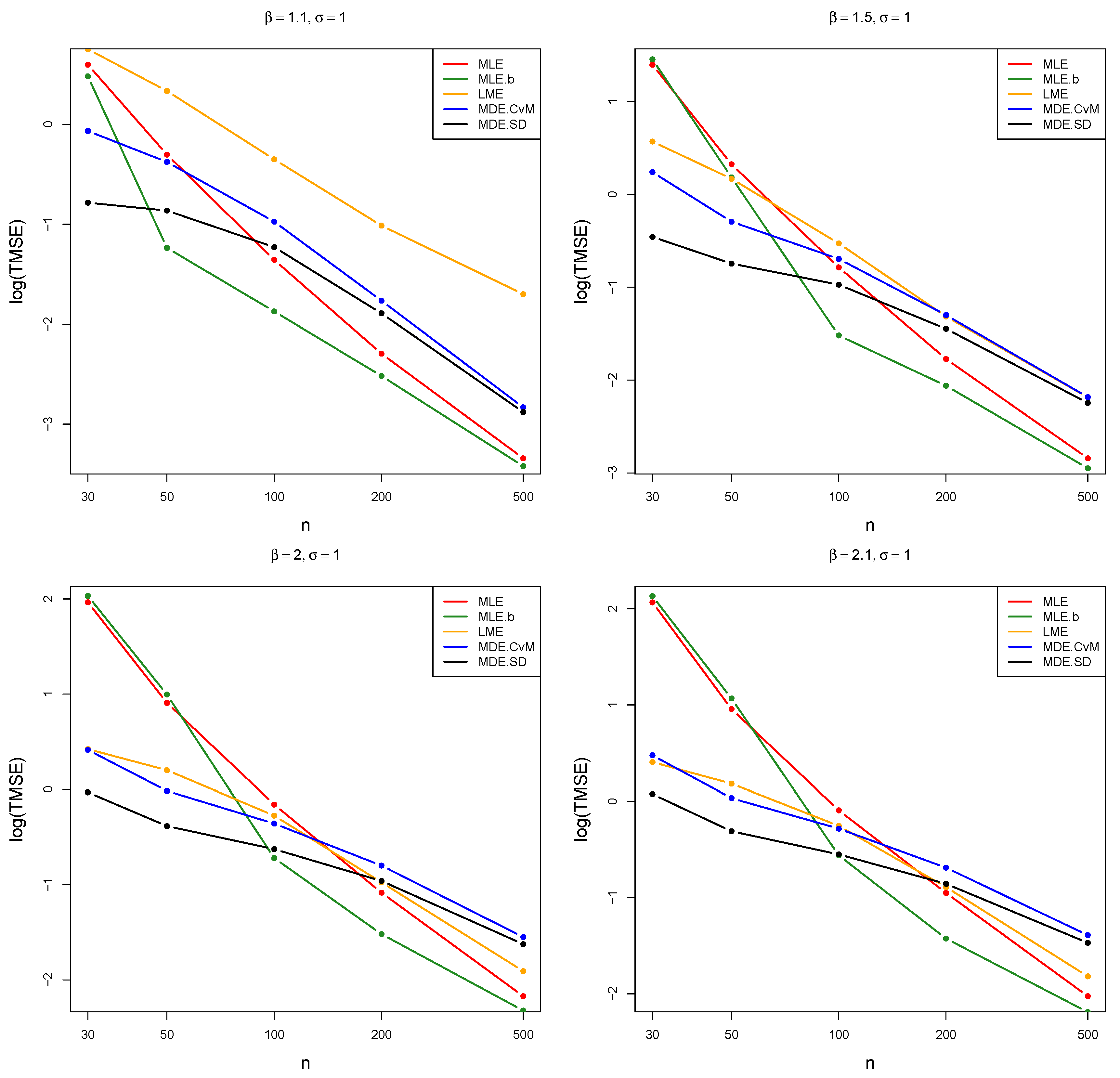
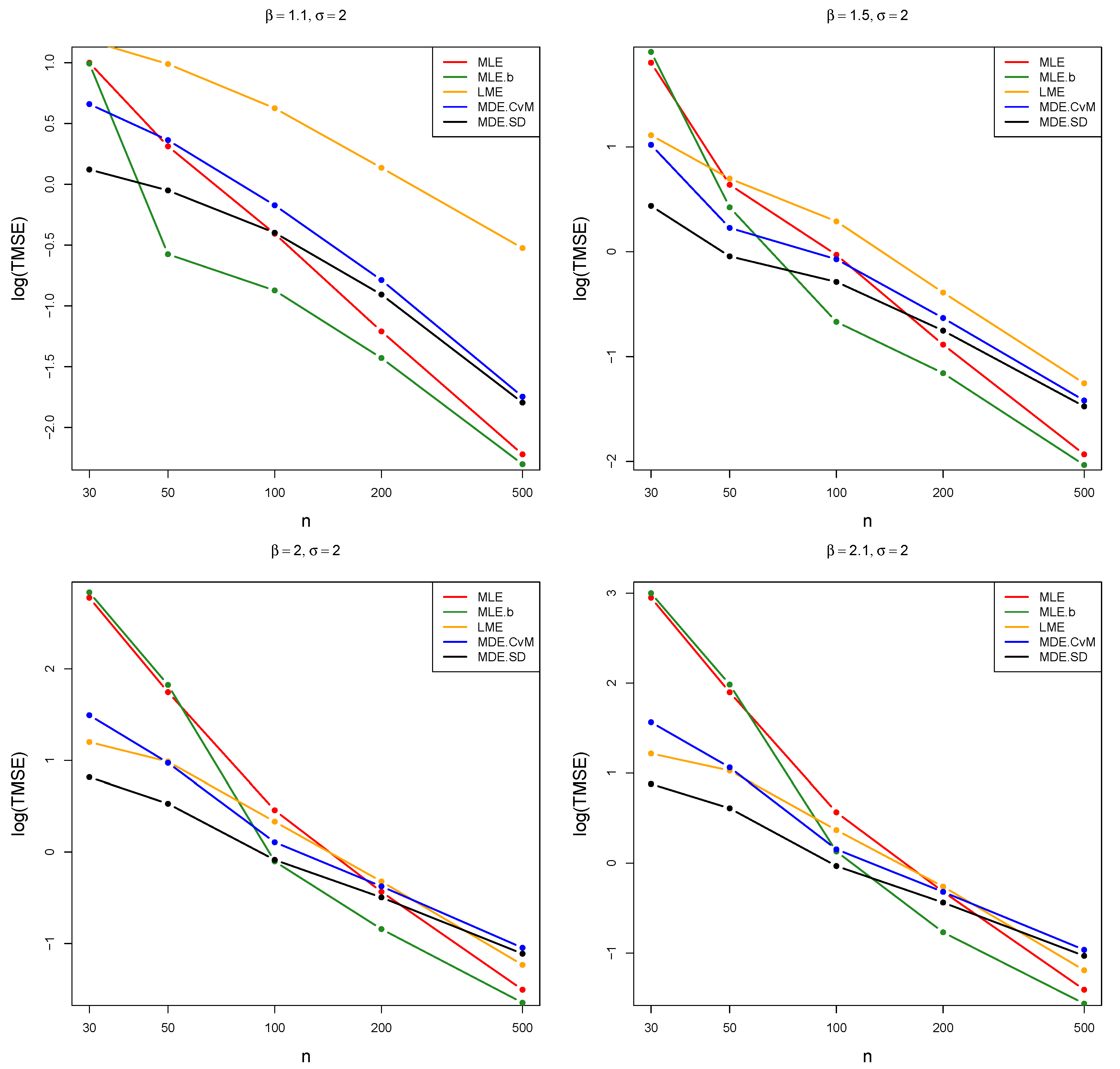
Figure 1 and Figure 2 show the logarithm of the TMSE as a function of sample size. We choose to use a logarithmic scale, as this increases the separation between the lines on the graph, which makes the figures easier to interpret.

Remark 3.

The reason for setting the number of Monte Carlo simulations to the relatively high number of 150,000 was due to the extreme sampling variation observed with the MLE and MLE.b estimators. This variability was exacerbated whenever using a particularly small sample size combined with a β value close to 2; therefore, we thought it best to make the number of simulations as large as possible in order to mitigate this issue. The variability is likely due to numerical issues related to the small sample sizes; note, however, that as the sample increases to $n=100$ and above this artefact disappears almost entirely. In addition, when considering the trimmed version of the measures calculated for each estimator in the simulation it is apparent that the sampling variability exhibited by these estimators is damped, which we feel is a more accurate reflection of the true value of these measures.

3.2. Results

To obtain a better understanding of the performance of the estimators considered in this study, we present a brief discussion of the simulation results presented in Table 1, Table 2, Table 3 and Table 4 and Table A1, Table A2, Table A3, Table A4, Table A5 and Table A6. We compare the trimmed versions of the variance, RB, and MSE performance of the estimators to one another in various parameter settings in the Monte Carlo study.

We start by first noting that the RB, variance, and MSE of each of the estimation methods improve when the sample size increases. The most notable improvements in overall MSE as the sample size increases from 30 to 500 are in the MLE, MDE.TV, and MME; however, as we mention later, the MME method should likely not be considered for estimation even for large samples. Interestingly, we find that the methods that perform well for smaller sample sizes do not always perform well for larger samples when compared to the competing methods. In particular, when the sample size is small ($n=30$ or $n=50$), it can be seen that in the majority of cases MDE.SD, MDE.CvM, and LME have the smallest variance, RB, and MSE values. Note that this small sample behaviour of the variance and MSE measures holds for all but the $\beta =1.1$ parameter. However, when considering the case in which the sample size is small and the parameter $\beta$ is specified to be small, there are instances where the MDE.CvM exhibits comparatively larger bias than MDE.SD, LME, and even MLE.b. Thus, it is clear that the underlying parameter values play a role in the relative performance of the various estimation techniques considered. Finally, when considering the RB for the various estimators, we note that MDE.SD most frequently gives rise to negative RB values for small samples. Based on the generally positive RB values associated with the remaining estimators, it seems that these other estimators tend to overestimate the true parameter value in these cases. This behaviour of MDE.SD (and indeed all other MDE-type estimators that we considered) is difficult to explain, as their distributional properties depend on the parameters and do not permit simple closed-form expressions.

Note that while MDE.KL, MDE.SD, and LME are relatively good estimators (in an MSE sense) when the sample size is large ($n=200$ or $n=500$), the MLE method now has the best performance among all methods considered in this setting.

Next, we consider the behaviour of the estimators as the parameter settings of the Monte Carlo change from one value to the next. As $\beta$ increases from 1.1 to 2, the values of the approximated variance, RB, and MSE of the estimators for both $\beta$ and $\sigma$ have the tendency to increase as well. However, these values then immediately start to decrease again when $\beta$ is strictly larger than 2.

When the value of $\sigma$ increases from 1 to 2, the simulation approximation of the variance of the estimators of $\sigma$ generally increases for all of the different estimation methods. The same is not necessarily true for the estimation of $\beta$, where we find that there are instances in which the approximated variance of the estimator of $\beta$ (using a given estimation method) decreases when the true $\sigma$ increases from 1 to 2, and increases in others.

When comparing the class of estimators based on minimum distance measures to the remaining methods, it can be readily seen that the MDE.SD and MDE.CvM estimators are the best performers in terms of the MSE for small to moderate samples. While LME is an excellent competitor, the MLE and MLE.b estimators perform relatively poorly in terms of the MSE in these cases. However, for larger sample sizes, the MLE and MLE.b clearly outperform the entire MDE class of estimators. Interestingly, the LME remains competitive here too, though it is almost never found to have the best MSE performance.

The performances of the estimators within the class of MDE methods differ wildly from one another. We have already noted that the MDE.SD and MDE.CvM methods generally have good MSE performance for small to moderate samples sizes; however, within this class we find that the MDE.TV and MDE.${\chi }^2$ are among the worst performances. The MDE.KL method is something of a mixed bag; certain parameter settings yield good MSE performance, while others yield extremely poor MSE performance. Generally, however, we can state that the MDE.KL method is a better performer than MDE.TV and MDE.${\chi }^2$, although this does not place this estimator near the top performers among the estimation methods considered.

The overall worst performing estimator is MME, regardless of which value of $\beta$ or $\sigma$ is considered. While this estimator improves with an increase in sample size, it nonetheless has the worst performance when compared to all other estimation methods.

In Figure 1 and Figure 2, the logarithm of the trimmed TMSE measure is plotted against the samples sizes in order to produce a more intuitive representation of the behaviour of a selection of estimators over varying sample sizes. The estimators MLE, MLE.b, LME, MDE.CvM, and MDE.SD are selected for inclusion in these figures, as according to the tables these estimators generally perform well (the TMSE and trimmed TMSE values of the remaining estimators can be found in the tables). It can be seen that, as expected, the trimmed TMSE measure’s value generally decreases as the sample size increases. Note, however, that the trimmed TMSE indicates that the MLE and MLE.b estimators are erratic for small samples (see for example the graphs associated with $\beta =2$ in Figure 1 and Figure 2). Furthermore, it is apparent that while the MLE and MLE.b estimators have among the worst trimmed TMSE performance for small sample sizes, this trend is reversed when the sample size increases. Conversely, it clear that the MDE.CvM and MDE.SD estimators perform well in terms of TMSE for smaller sample sizes, in many cases being outperformed only when the sample size increases to $n=100$ and higher. It should be noted that while the performance of LME is comparable to the performance of MDE.CvM for choices of $\beta$ larger than 2, it performs poorly for smaller $\beta$ values. Furthermore, these numerical results indicate that the relative performance of the estimators depends to a certain degree on the specific parameter values considered.

4. Practical Applications

We now apply the various Lomax parameter estimation techniques to a practical data set, namely, the airborne communication transceiver data shown in

Table 5. Repair times for the airborne communication transceiver dataset.

0.2	0.3	0.5	0.5	0.5	0.5	0.6	0.6	0.7	0.7	0.7	0.8
0.8	1.0	1.0	1.0	1.0	1.1	1.3	1.5	1.5	1.5	1.5	2.0
2.0	2.2	2.5	2.7	3.0	3.0	3.3	3.3	4.0	4.0	4.5	4.7
5.0	5.4	5.4	7.0	7.5	8.8	9.0	10.3	22.0	24.5

, originally discussed in [41], and previously analysed in [22].

The dataset contains 46 observed repair times (measured in hours) of airborne communication transceiver equipment recorded during active operation. Assuming a Lomax distribution for these data, we use each of the estimation techniques to obtain the parameter estimates of the distribution. The resulting parameter estimates, along with 95% parametric bootstrap confidence intervals using $B=1000$ bootstrap replications, are shown in

Table 6. Estimated parameters for the airborne communication transceiver dataset (with a 95% percentile bootstrap confidence interval).

Estimation Technique	$\widehat{\mathit{\beta }}$	${\mathbf{CI}}_{0.95}$	$\widehat{\mathit{\sigma }}$	${\mathbf{CI}}_{0.95}$
MLE	$3.549$	$[1.540;56.744]$	$9.236$	$[2.672;166.270]$
MLE.b	$3.549$	$[1.222;43.509]$	$9.236$	$[1.792;138.151]$
LME	$3.387$	$[1.692;16.621]$	$8.608$	$[3.171;52.699]$
MDE.CvM	$4.105$	$[0.965;34.123]$	$10.685$	$[1.223;112.835]$
MDE.SD	$3.399$	$[0.933;26.084]$	$8.670$	$[1.312;78.789]$
MDE.${\chi }^2$	$1.820$	$[0.583;19.904]$	$7.706$	$[5.077;178.639]$
MDE.TV	$2.402$	$[0.819;105.179]$	$9.732$	$[5.293;920.561]$
MDE.KL	$3.549$	$[1.474;52.620]$	$9.236$	$[2.653;191.968]$
MME	$4.385$	$[2.603;81.117]$	$12.209$	$[6.540;290.507]$

. Note that for each estimation method the parametric bootstrap samples used in these intervals are constructed by first estimating the parameters and then generating samples from a Lomax distribution with the estimators as the parameters [42]. The output in Table 6 indicates that the estimated parameter values are all reasonably close to one another, with the exception of MDE.CvM, MDE.${\chi }^2$, MDE.TV, and MME. The discrepancies observed for these four estimators relative to the other estimators considered is perhaps unsurprising in light of the irregular performance of these estimators observed in the Monte Carlo study presented earlier.

The code for this example can be found here: https://tinyurl.com/LomaxPracticalCode (accessed on 26 November 2023).

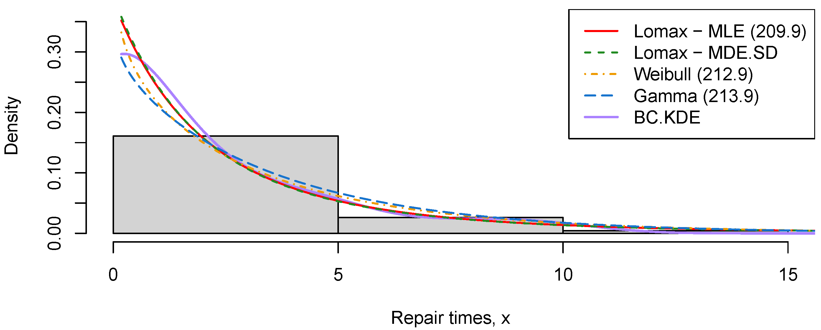
Figure 3 shows the boundary-corrected kernel density estimator (BC.KDE) of the data (obtained using the bckden suite of functions in R’s evmix package [43]) overlaid on a simple histogram. Two separate Lomax density functions are added to the plot using two different methods of parameter estimation, namely, MLE and MDE.SD, the latter being chosen because this method performed well for smaller sample sizes. In addition, the fitted two-parameter Weibull and gamma densities are added to the plot in order to facilitate comparison between the Lomax density and other theoretical densities containing two parameters. The parameters from both of these theoretical densities are estimated via maximum likelihood. Visual inspection of the graph indicates that the Lomax densities can be considered good candidate models, as they most closely match the empirical estimate of the density of these data, whereas the gamma distribution exhibits the greatest deviation from the others.

The Akaike information criterion (AIC) is calculated for each of the three distinct distributions by employing the maximum likelihood estimators, with the results presented in

Table 7. The AIC values for the fitted distributions of the airborne communications transceiver data.

Weibull	Gamma	Lomax ${}^{\ast }$
212.9	213.9	209.9

* The AIC value reported for the Lomax distribution employs the MLE.

. From Table 7, it can be seen that the Lomax distribution has the lowest AIC value, closely followed by the AIC of the Weibull and gamma distributions, which supports the conclusions made above.

5. Conclusions

In this study, different parameter estimation methods for the two parameters of the Lomax distribution have been explored and discussed. We have reviewed L-moment estimators, maximum likelihood estimators (with and without a bias adjustment), method of moments estimators, and three different minimum distance estimators. The specific goals of the study were to provide an overview of the different estimation methods as well as to determine whether the minimum distance estimators are feasible estimation alternatives for this distribution when compared to traditional methods of estimation such as maximum likelihood. In an attempt to ascertain the properties of these estimators, all of the methods were compared to one another in a comprehensive Monte Carlo simulation while assuming different parametric values for small to large samples. Unsurprisingly, this study showed that while the MLEs perform well in large samples, they yield severely biased answers in small samples. The bias correction outlined in [14], however, noticeably reduces the bias of the MLE estimates for moderate to large sample sizes.

The traditional MME is found to be a universally poor performer in terms of MSE for all settings of the $\beta$ and $\sigma$ parameters and the given sample sizes. Our simulation showed that LME is stable under different parameter settings, including varying values of $\beta$, $\sigma$, and sample size. Thus, while this estimator is almost never found to have the best performance in either small or large sample settings, it can be considered a ‘safe’ option for estimating of the parameters of the Lomax distribution.

Finally, several estimation methods based on distance measures were investigated, and were found to produce varied results. These methods all attempt to estimate the parameters of the Lomax distribution by considering different measures of distance measures that need to be minimised. The studied measures considered include the Cramér–von Mises (CvM), squared difference, and several phi-divergence measures (including the Kullback–Leibler (KL) divergence, total variation (TV) distance, and chi-square divergence). The results of the simulation study established that, for this class of MDE methods, the MDE.SD and MDE.CvM methods have the best overall MSE performance for small to moderate samples sizes; we would recommend either of these methods for the estimation of the Lomax parameters $\sigma$ and $\beta$ when sample sizes are smaller than 100. However, within this MDE class we find two of the worst performing methods, namely, the MDE.TV and MDE.${\chi }^2$ methods. The MDE.KL method produces reasonably good MSE performance for the moderate to large sample sizes, however, as with MLE, the quality of the estimator fluctuates tremendously for smaller samples.

These results show that while no single estimator has the best overall performance, we can identify the distance-based measure, that is, MDE.SD, as generally having the best MSE performance for small sample sizes ($n=30$ and $n=50$), whereas MLE.b is found to be the better choice for moderate and large sample sizes ($n=100$, $n=200$ and $n=500$) for almost all of the $\sigma$ and $\beta$ values considered here.

The related literature contains finds competing views about the usefulness of MDEs and MLEs. In the case of multivariate data (specifically estimators for the parameters of a copula), [44] advocates for the use of MDEs because MLEs have the disadvantage that of requiring the density of the copula, whereas MDEs only require its empirical distribution estimate. However, in an extensive overview paper comparing MDEs and MLEs for parameter estimation of copulas, [45] found that MLEs have a lower computational cost while producing lower estimation biases. Naturally, the other main advantages of the traditional MLEs are the ease with which asymptotic standard errors can be obtained, the fact that they have asymptotically normal distributions, and, consequently, that confidence intervals for the parameter being estimated are easy to obtain. In contrast, the standard errors of the other estimators considered in this paper require either complex analytical derivations (possibly with no tractable forms) or require the use of resampling methods.

Finally, we note that another important application of the Lomax distribution, not mentioned yet in this paper, is found in autoregressive conditional duration (ACD) models, which model high frequency financial data; in this context, the duration between market events are of great interest. Without discussing the details of the model, we briefly describe the role of the Lomax distribution in ACD models here; for an in-depth exposition of ACD models, see [46,47]. We only note that the error terms of the ACD model are historically assumed to be exponential or Weibull distributed; see, for example, [48]. However, in [49,50], it is found that these choices do not adequately describe the characteristics of the observed data. In [51], the authors advocate the use of infinite mixtures of exponential distributions to model the distribution of the error term, finding that this choice improves the fit of the model. If the scale parameter of this mixing exponential distribution follows an inverse Gaussian distribution, then the resulting distribution of the error term is Lomax. It is therefore important for the efficient implementation of these ACD models that we are able to accurately estimate the parameters of this distribution. Another important avenue for future research can be found in goodness-of-fit tests for the Lomax and related distributions, as these tests check the assumptions underlying the ACD models.

References

- Pareto, V. The new theories of economics. J. Political Econ. 1897, 4, 485–502. [Google Scholar] [CrossRef]
- Lomax, K. Business failures: Another example of the analysis of failure data. J. Am. Stat. Assoc. 1954, 49, 847–852. [Google Scholar] [CrossRef]
- Mitra, D.; Kundu, D.; Balakrishnan, N. Likelihood analysis and stochastic EM algorithm for left truncated right censored data and associated model selection from the Lehmann family of life distributions. Jpn. J. Stat. Data Sci. 2021, 4, 1019–1043. [Google Scholar] [CrossRef]
- Abujarad, M.H.A.; Khan, A.A. JMASM 57: Bayesian Survival Analysis of Lomax Family Models with Stan (R). J. Mod. Appl. Stat. Methods 2021, 19, 12. [Google Scholar] [CrossRef]
- Atkinson, A.B.; Harrison, A.J. Distribution of Personal Wealth in Britain; Cambridge University Press: Cambridge, UK, 1978. [Google Scholar]
- Harris, C.M. The Pareto distribution as a queue service discipline. Oper. Res. 1968, 2, 307–308. [Google Scholar] [CrossRef]
- Hassan, A.; Al-Ghamdi, A. Optimum step-stress accelerated life testing for Lomax distribution. J. Appl. Sci. Res. 2009, 12, 2153–2164. [Google Scholar]
- Holland, O.; Golaup, A.; Aghvami, A.H. Traffic characteristics of aggregated module downloads for mobile terminal reconfiguration. IEE Proc. 2006, 135, 683–690. [Google Scholar] [CrossRef]
- Hosking, J.R.M.; Wallis, J.R. Parameter and quantile estimation for the generalized Pareto distribution. Technometrics 1987, 29, 339–349. [Google Scholar] [CrossRef]
- de Zea Bermudez, P.; Kotz, S. Parameter estimation of the generalized Pareto distribution—Part I. J. Stat. Plan. Inference 2010, 140, 1353–1373. [Google Scholar] [CrossRef]
- Ramos, P.L.; Nascimento, D.C.; Ferreira, P.H.; Weber, K.T.; Santos, T.E.G.; Louzada, F. Modelling traumatic brain injury lifetime data: Improved estimators for the generalised gamma distribution under small samples. PLoS ONE 2019, 14, e0221332. [Google Scholar] [CrossRef] [Green Version]
- Teimouri, M.; Hoseini, S.M.; Nadarajah, S. Comparison of estimation methods for the Weibull distribution. Statistics 2013, 47, 93–109. [Google Scholar] [CrossRef]
- Dey, S.; Menezes, F.B.; Mazucheli, J. Comparison of estimation methods for unit-gamma distribution. J. Data Sci. 2019, 17, 768–801. [Google Scholar] [CrossRef]
- Giles, D.E.; Feng, H.; Godwin, R.T. On the bias of the maximum likelihood estimator for the two-parameter Lomax distribution. Commun. Stat. Methods 2013, 42, 1934–1950. [Google Scholar] [CrossRef] [Green Version]
- Shakeel, M.; Rehmat, N.; Haq, M.A. Comparison of the robust parameters estimation methods for the two-parameters Lomax distribution. Cogent Math. 2017, 4, 3–5. [Google Scholar] [CrossRef]
- Juaŕez, S.F.; Schucany, W.R. Robust and efficient estimation for the generalized Pareto distribution. Extremes 2004, 7, 237–251. [Google Scholar] [CrossRef]
- Basu, A.; Harris, I.R.; Hjort, N.L.; Jones, M.C. Robust and efficient estimation by minimising a density power divergence. Biometrika 1998, 85, 549–559. [Google Scholar] [CrossRef] [Green Version]
- Basu, A.; Shioya, H.; Park, C. Statistical Inference: The Minimum Distance Approach; Chapman and Hall: Boca Raton, FL, USA, 2011. [Google Scholar]
- Boos, D. Minimum distance estimators for location and goodness of fit. J. Am. Stat. Assoc. 1981, 76, 663–670. [Google Scholar] [CrossRef]
- Parr, W.C.; Schucany, W.R. Minimum distance and robust estimation. J. Am. Stat. Assoc. 1980, 75, 616–624. [Google Scholar] [CrossRef]
- Parr, W.C.; De Wet, T. On minimum Cramer-von Mises-norm parameter estimation. Commun. Stat. Methods 1981, 10, 1149–1166. [Google Scholar] [CrossRef]
- Ferreira, P.H.; Ramos, R.; Ramos, P.L.; Gonzales, J.F.B.; Tomazella, V.L.D.; Ehlers, R.S.; Silva, E.B.; Louzada, F. Objective Bayesian analysis for the Lomax distribution. Stat. Probab. Lett. 2020, 159, 108677. [Google Scholar] [CrossRef] [Green Version]
- He, D.; Sun, D.; Zhu, Q. Bayesian analysis for the Lomax model using noninformative priors. Stat. Theory Relat. Fields 2022, 1–8. [Google Scholar] [CrossRef]
- Son, Y.S.; Oh, M. Bayesian estimation of the two-parameter gamma distribution. Commun. Stat. Comput. 2006, 35, 285–293. [Google Scholar] [CrossRef]
- Hosking, J.R.M. L-moments: Analysis and estimation of distributions using linear combinations of order statistic. J. R. Stat. Soc. 1990, 52, 105–124. [Google Scholar] [CrossRef]
- Hosking, J.R.M. Maximum-likelihood estimation of the parameters of the generalized extreme-value distribution. J. R. Stat. Society. Ser. C Appl. Stat. 1985, 34, 301–310. [Google Scholar]
- Greenwood, J.A.; Landwehr, J.M.; Matalas, N.C.; Wallis, J.R. Probability weighted moments:Definition and relation to parameters of several distributions expressable in inverse form. Water Resour. Res. 1979, 52, 105–124. [Google Scholar]
- Asquith, W. Univariate Distributional Analysis with L-moment Statistics Using R; Create Space Independent Platform: Scotts Valley, CA, USA, 2011. [Google Scholar]
- Deville, Y. Renext: Renewal Method for Extreme Values Extrapolation, R package version 3.1-0; Institut de Radioprotection et de Sûreté Nucléaire: Fontenay-aux-Roses, France, 2016. [Google Scholar]
- R Core Team. R: A Language and Environment for Statistical Computing; R Foundation for Statistical Computing: Vienna, Austria, 2021. [Google Scholar]
- Cheng, R.; Amin, N. Maximum product of spacings estimation with application to the lognormal distribution. Math. Rep. 1979, 1, 79. [Google Scholar]
- Ranneby, B. The maximum spacing method. An estimation method related to the maximum likelihood method. Scand. J. Stat. 1984, 11, 92–112. [Google Scholar]
- Wolfowitz, J. Estimation by the minimum distance method. Ann. Inst. Stat. Math. 1953, 5, 9–23. [Google Scholar]
- Beran, R.J. Minimum Pareto distance estimates for parameter models. Ann. Stat. 1977, 5, 445–463. [Google Scholar] [CrossRef]
- Beran, R.J. An efficient and robust adaptive estimator of location. Ann. Stat. 1978, 6, 292–313. [Google Scholar]
- Broyden, C.G. The convergence of a class of double-rank minimization algorithms. J. Inst. Math. Its Appl. 1970, 6, 76–90. [Google Scholar] [CrossRef] [Green Version]
- Fletcher, R. A New Approach to Variable Metric Algorithms. Comput. J. 1970, 13, 317–322. [Google Scholar] [CrossRef] [Green Version]
- Goldfarb, D. A Family of Variable Metric Updates Derived by Variational Means. Math. Comput. 1970, 24, 23–26. [Google Scholar] [CrossRef]
- Shanno, D.F. Conditioning of quasi-Newton methods for function minimization. Math. Comput. 1970, 24, 647–656. [Google Scholar] [CrossRef]
- Silverman, B.W. Density Estimation for Statistics and Data Analysis; Chapman & Hall, Inc.: London, UK, 1986. [Google Scholar]
- Von Alven, W.H. Reliability Engineering; Prentice Hall: Hoboken, NJ, USA, 1964. [Google Scholar]
- Efron, B.; Tibshirani, R.J. An Introduction to the Bootstrap; Chapman & Hall, Inc.: New York, NY, USA, 1993. [Google Scholar]
- Hu, Y.; Scarrott, C. evmix: An R package for Extreme Value Mixture Modeling, Threshold Estimation and Boundary Corrected Kernel Density Estimation. J. Stat. Softw. 2018, 84, 1–27. [Google Scholar] [CrossRef] [Green Version]
- Liebscher, E.; Taubert, F.; Hetzer, J. Modelling multivariate data using product copulas and minimum distance estimators: An exemplary application to ecological traits. Environ. Ecol. Stat. 2022, 29, 1–24. [Google Scholar] [CrossRef]
- Weiss, G. Copula parameter estimation by maximum-likelihood and minimum-distance estimator: A simulation study. Comput. Stat. 2011, 26, 31–54. [Google Scholar] [CrossRef]
- Engle, R.F.; Russell, J.R. Autoregressive conditional duration: A new model for irregularly spaced transaction data. Econometrica 1998, 66, 1127–1162. [Google Scholar] [CrossRef] [Green Version]
- Thas, O. Comparing Distributions; Springer: New York, NY, USA, 2010. [Google Scholar]
- Meintanis, S.G.; Milosevic, B.; Obradovic, M. Goodness-of-fit tests in conditional duration models. Stat. Pap. 2020, 61, 123–140. [Google Scholar] [CrossRef]
- Bauwens, L.; Giot, P. Econometric Modelling of Stock Market Intraday Activity; Kluver Academic Publisher: Boston, MA, USA, 2001. [Google Scholar]
- Bauwens, L.; Giot, P.; Grammig, J.; Veredas, D. A comparison of financial duration models via density forecasts. Int. J. Forecast. 2005, 20, 589–609. [Google Scholar] [CrossRef]
- De Luga, G.; Gallo, G.M. Mixture processes for financial intradaily durations. Stud. Nonlinear Dyn. Econom. 2004, 8. [Google Scholar] [CrossRef]
Figure 1.
Plots of the log of the trimmed TMSE measure against sample size for five different estimation techniques when .
Figure 2.
Figure 3.
The kernel density estimate and fitted density functions based on the airborne communication transceiver repair time data (AIC values for the MLE estimated distributions provided in parentheses in the legend).