


Solutions of the Yang–Baxter Equation and Automaticity Related to Kronecker Modules
by
 ,
,
Agustín Moreno Cañadas
1,*,† ,
,
Pedro Fernando Fernández Espinosa
2,† and
Adolfo Ballester-Bolinches
3,† 1
Departamento de Matemáticas, Universidad Nacional de Colombia, Edificio Yu Takeuchi 404, Kra 30 No 45-03, Bogotá 11001000, Colombia
2
Departamento de Matemáticas, Universidad de Caldas, Cll 65 No 26-10, Manizales 170004, Colombia
3
Departament de Matemàtiques, Universitat de València, Dr. Moliner 50, Burjassot, 46100 València, Spain
*
Author to whom correspondence should be addressed.
†
These authors contributed equally to this work.
Computation 2023, 11(3), 43; https://doi.org/10.3390/computation11030043
Submission received: 17 January 2023
/
Revised: 6 February 2023
/
Accepted: 17 February 2023
/
Published: 21 February 2023
(This article belongs to the Special Issue Graph Theory and Its Applications in Computing)
Abstract
:The Kronecker algebra is the path algebra induced by the quiver with two parallel arrows, one source and one sink (i.e., a quiver with two vertices and two arrows going in the same direction). Modules over are said to be Kronecker modules. The classification of these modules can be obtained by solving a well-known tame matrix problem. Such a classification deals with solving systems of differential equations of the form , where A and B are , -matrices with an algebraically closed field. On the other hand, researching the Yang–Baxter equation (YBE) is a topic of great interest in several science fields. It has allowed advances in physics, knot theory, quantum computing, cryptography, quantum groups, non-associative algebras, Hopf algebras, etc. It is worth noting that giving a complete classification of the YBE solutions is still an open problem. This paper proves that some indecomposable modules over called pre-injective Kronecker modules give rise to some algebraic structures called skew braces which allow the solutions of the YBE. Since preprojective Kronecker modules categorize some integer sequences via some appropriated snake graphs, we prove that such modules are automatic and that they induce the automatic sequences of continued fractions.
Keywords:
automatic sequence; brace; Kronecker module; matrix problem; path algebra; Yang–Baxter equationMSC:
11B85; 16T25; 16G30; 16G601. Introduction
An automorphism R over a vector space V is a solution of the Yang–Baxter equation, if it satisfies the following identity (1) known as the braided equation, i.e.,
is satisfied on .
Equation (1) was introduced in 1967 by Yang in two short papers written with the purpose of generalizing previous works on theoretical physics. Shortly afterwards, Baxter introduced such an equation in a paper regarding statistical mechanics. It is worth noting that giving a complete classification of the YBE solutions remains an open problem [1,2].
YBE research is a trending topic in several fields of mathematics. Its investigation has influenced areas such as Hopf algebras, quantum computing, cryptography, knot theory, non-associative algebras, etc. For instance, Civino et al. [3] used the cryptanalysis of substitution–permutation networks to give a non-degenerate involutive set-theoretical solutions of the YBE via some algebraic structures named braces. YBE was used by Chen [4] to generate braiding quantum gates helpful in topological quantum computing and Kauffman et al. [5] proved that the solutions of the YBE give rise to universal gates in a quantum computer.
It is worth pointing out that Nichita et al. [6,7,8] introduced the Yang–Baxter operators of the form , such that , where for a field , is a unitary associative -algebra. Furthermore,
- if ;
- if ;
- if .
In particular, gives the universal quantum gate
Nichita [7] defined another Yang–Baxter operator, which generate identities in Jordan algebras after appropriated specializations.
On the other hand, the representation theory of the Kronecker algebra is a subject of great interest in the matrix problem theory. Kronecker and Weierstrass found out the indecomposable modules associated with this algebra by solving the following matrix problem over an algebraically closed field [9,10,11]. In this case, we denote by , , , a matrix M (called Kronecker matrix) consisting of two matrix blocks X and Y with the same size, the ith row of the matrix M, and the jth (kth) column of the matrix block X (Y).
| Kronecker Problem |
Finding the canonical Jordan forms of matrices of type M with respect to the following transformations:
- Row permutations;
- Additions of the form , with , ;
- Simultaneous column permutations of and within the matrix block X, and and within the matrix block Y;
- Multiplications of the form , where .
If the Kronecker matrices and can be transformed one into the other by means of elementary transformations, then they are said to be equivalent or isomorphic as Kronecker modules.
Recently, Espinosa [12] found new invariants associated with preprojective and pre-injective Kronecker modules (i.e., non-regular Kronecker modules) in their investigations regarding the categorization of real sequences in the sense of Ringel et al. [13,14]. So-called Kronecker snake graphs are examples of such invariants. This paper proves that some snake graphs arising from pre-injective Kronecker modules (called helices or pre-injective Kronecker snake graphs) induce skew braces. In other words, we prove that appropriated snake graphs associated with indecomposable Kronecker modules induce the solutions of YBE.
Automaticity associated with different algebraic structures is a widely studied topic. The seminal work by Turing regarding the classification of numbers is perhaps one of the most remarkable works regarding this subject [15]. He classified real numbers as computable or uncomputable. Accordingly, computable numbers are real numbers whose k-adic expansion () can be produced by a Turing machine. It is worth noting that automata are one of the most basic computation models, and that if a sequence is generated by a k-automaton, then the sequence is said to be automatic [16,17].
According to Shallit et al. [17], automatic sequences have strong relationships with number theory. These interactions allow many results in transcendence theory to be proven with positive characteristics. In particular, Adamczewski et al. [18] proved that Liouville numbers cannot be generated by a finite automaton, thus answering a conjecture proposed by Shallit [16].
Relationships between the theory of the representation of algebras and the automata theory were given by Rees [19], who proved that strings and bands (associated with indecomposable modules over monomial algebras) can be generated by an automaton. In this paper, it is proven that the preprojective Kronecker modules give rise to some automatic categories and that the sequences of some continued fractions associated with such modules are automatic.
1.1. Motivations
Since their introduction, Kronecker modules have been a source of a plethora of applications in diverse science fields [10,11]. Particularly, these have been used to solve differential equations [20]. The generalizations of the Kronecker matrix problem give rise to the well-known Krawtchouk matrices with applications in quantum computing, statistics, combinatorics, coding theory, probability, etc. [21]. On the other hand, relationships between automata theory, the number theory, and the theory of representation of algebras is a topic of great interest among many mathematicians [16,17].
It is worth noting that the categorization of integer sequences in the sense of Ringel et al. [13,14] allows interpreting numbers in sequences as the invariants of objects of a given category (for instance, modules over path algebras or quiver representations). Automatic sequences give rise to automatic objects in these categories. This paper proves that integer sequences categorized by preprojective Kronecker modules are automatic.
1.2. Contributions
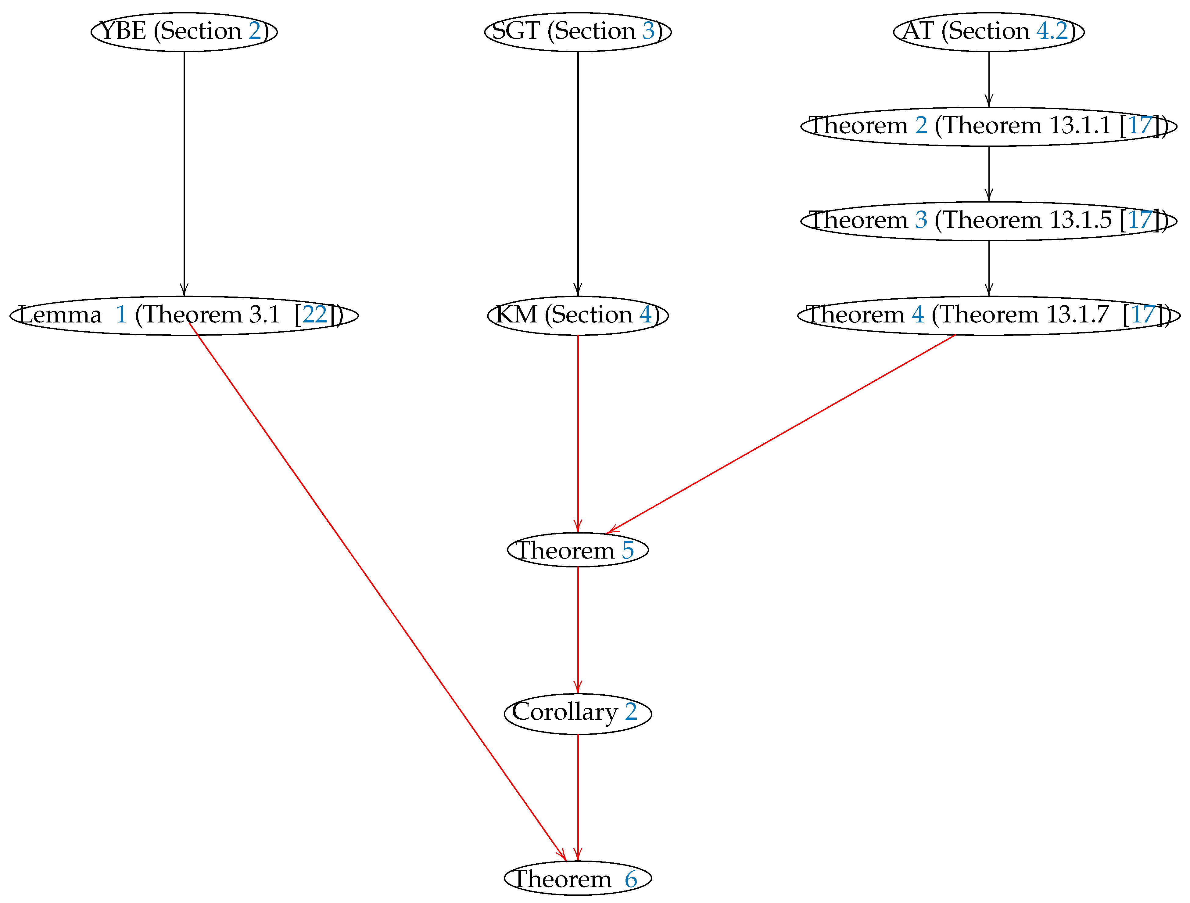
The main results of this paper are Theorem 5, Corollary 2, and Theorem 6. These are illustrated as the targets of red arrows in Figure 1, which shows how the different theories are related to each other to obtain our results. We use the acronyms AT, Cr, KM, Lm, Sect, SGT, Th, and YBE for automata theory, corollary, Kronecker modules, lemma, section, snake graph theory, theorem and Yang–Baxter equation, respectively.
Theorem 5 proves that the categories of type generated by a finite number of preprojective Kronecker modules are automatic. Corollary 2 proves that some sequences of continued fractions (arising from the preprojective Kronecker modules) are automatic. Theorem 6 proves that pre-injective Kronecker modules give rise to skew braces which, according to Vendramin et al. [22], generate solutions of the YBE.
The organization of this paper is as follows: the main definitions and notations are given in Section 2; we reiterate the definitions and notations regarding YBE in Section 2; the snake graphs are shown in Section 3; the Kronecker modules are elaborated in Section 4; and the automatic sequences and automatic categories are discussed in Section 4.2 and Section 4.3. Finally, we present the main results in Section 5 and the concluding remarks are given in Section 6.
Figure 1.
The main results presented in this paper (targets of red arrows) allow a connection to be established between YBE theory, the representation theory of the Kronecker algebra, the automata theory, and the snake graph theory. We use the acronyms AT, Cr, KM, Lm, Sect, SGT, Th, and YBE for automata theory, corollary, Kronecker modules, lemma, section, snake graph theory, theorem, and Yang–Baxter equation, respectively.

2. Preliminaries
This section recalls some basic definitions and results regarding YBE, braces, and Kronecker modules, which are helpful for a better understanding of this paper.
Yang–Baxter Equation and Its Solutions
This section makes a brief introduction to some of the methods used to solve the YBE [6,7,8,23,24,25,26,27].
Drinfeld [28] proposed that the set-theoretical YBE be solved. Solutions of these kinds of equations are given by quadratic sets, which are pairs of the form , where X is a set and is a bijective map that satisfies the corresponding braided Equation (2).
meaning that a solution written as , for all is said to be non-degenerate, provided that and are bijective maps for any . It is involutive if [24].
One of the best approaches to solve the non-degenerate involutive set-theoretical solutions of the YBE was introduced by Rump [25,26], who define some algebraic structures called braces. According to Cedó, Jespers and Oknińiski [23], a left brace is an Abelian group endowed with another group structure, defined by a rule that satisfies the compatibility conditions for all .
Right braces are defined in the same fashion. In such a case, the compatibility condition has the form .
Note that, if X is finite, then an involutive solution of the braided equation is right non-degenerate if and only if it is left non-degenerate. It is worth noticing that the non-degenerate involutive set-theoretical solutions of the YBE were given by Etingof et al. and Gateva-Ivanova and Van den Bergh [29,30] by associating a group with the solution [23]. Afterwards, Ballester-Bolinches et al. [27] used the Cayley graph of some subgroups (of the symmetric group on X denoted ) associated with the solutions of the YBE to define the left braces.
For , we define by
Rump proved the following result.
Lemma 1
- 1.
- ;
- 2.
- ;
- 3.
- The map defined by is a non-degenerate involutive set-theoretical solution of the YBE.
We remind that Vendramin and Guarnieri [22] introduced the notion of skew brace. According to them, a skew left brace A is a group (written multiplicatively) with an additional group structure given by such that
holds for all , where denotes the inverse of a with respect to the group structure given by .
Left braces are examples of skew braces.
The following results describes the non-degenerate involutive set-theoretical solutions of the YBE in terms of skew braces.
Theorem 1
(Theorem 3.1. [22]). Let A be a skew left brace. Then, , is a non-degenerate solution of the YBE. Furthermore, is involutive if and only if for all .
3. Snake Graphs
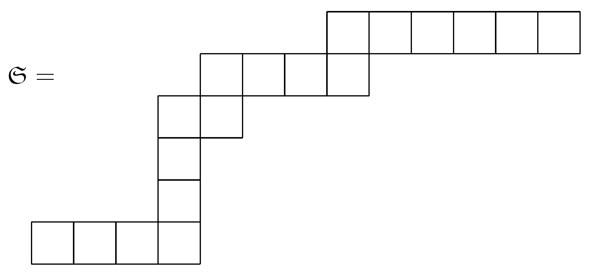
Snake graphs are finite-connected planar graphs consisting of uniform adjacent square tiles. Two consecutive tiles and are cemented by gluing either the northern edge of with the southern edge of or the eastern edge of with the western edge of [31,32,33].
A snake graph is said to be horizontal straight (vertical straight) if the gluing process is only applied to the eastern–western edges (northern–southern) of its tiles. Any snake graph is a union of a finite number of straight snake graphs , if , then we write . Figure 2 shows an example of the snake graph .
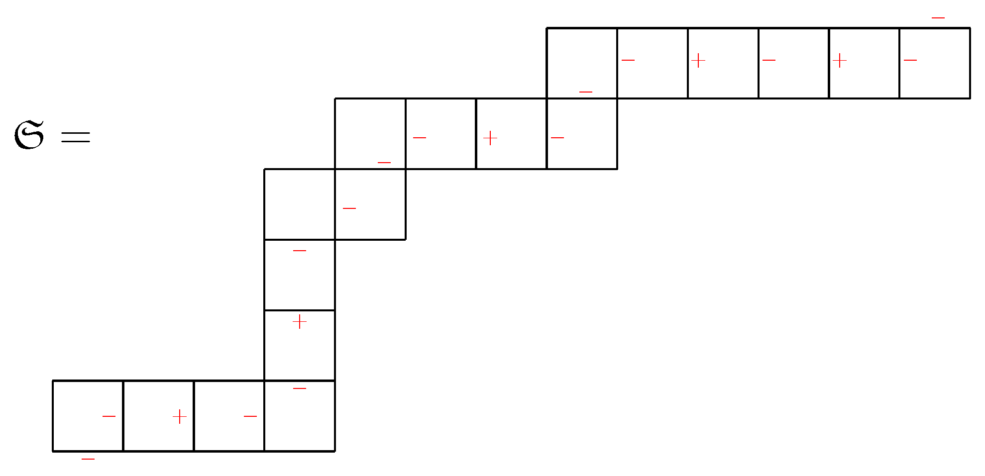
According to Schiffler et al. [31,32,33], if a snake graph consists of tiles . Then, there is an associated sequence of functions , such that , , , where , , , denote the west, south, east, and north edges of tile , respectively.
Note that the values of given by the internal edges, , , , and tiles completely determine the snake graph . For instance, if , then , and . Figure 3 shows an example of a sequence associated with the snake graph .
A positive finite continued fraction is a function
on n variables , .
Positive continued fractions are determined by their convergents denoted by , . Note that n is finite if and only if the continued fraction gives a rational number denoted by .
Schiffler et al. [31,32,33] proved that there is a bijective correspondence between the set of positive continued fractions and the set of snake graphs via sequence . They denoted by the unique snake graph defined by the continued fraction . As an example, the snake graph of the continued fraction is , as shown in Figure 3.
4. The Kronecker Problem
This section describes the solutions to the Kronecker problem formulated in the introduction. Snake graphs are invariants associated with such solutions.
The Kronecker problem was solved by Weierstrass in 1867 for some particular cases and by Kronecker in 1890 for the complex numbers field case. Solutions to this problem are classified as regular or non-regular (preprojective or pre-injective) [9,10,11].
Solutions to the Kronecker problem correspond to the indecomposable modules over the algebra , where is a field and the multiplication is given by the formula
Finite dimensional right -modules are called Kronecker modules, and every such a module can be identified with a quadruple , where and are the vector spaces , , and are linear maps defined by , , for , and is the standard basis of .
The category of Kronecker modules is categorically equivalent to the category of Kronecker matrices, so indecomposable Kronecker modules can be determined by solving the Kronecker matrix problem described in the introduction of this paper. Two Kronecker matrices and are said to be equivalent (or isomorphic as Kronecker modules) if one can be obtained from the other via matrix transformations.
It is worth noting that the Auslander–Reiten quiver associated with the Kronecker algebra has three components, which are the preprojective component containing all the indecomposable projective modules; the pre-injective component containing all the indecomposable injective modules; and the regular component. We let () denote a preprojective Kronecker module (pre-injective Kronecker module) whose associated Kronecker matrix has (n) rows and n () columns. The following matrices () show the standard form of the canonical pre-injective (preprojective) Kronecker modules.
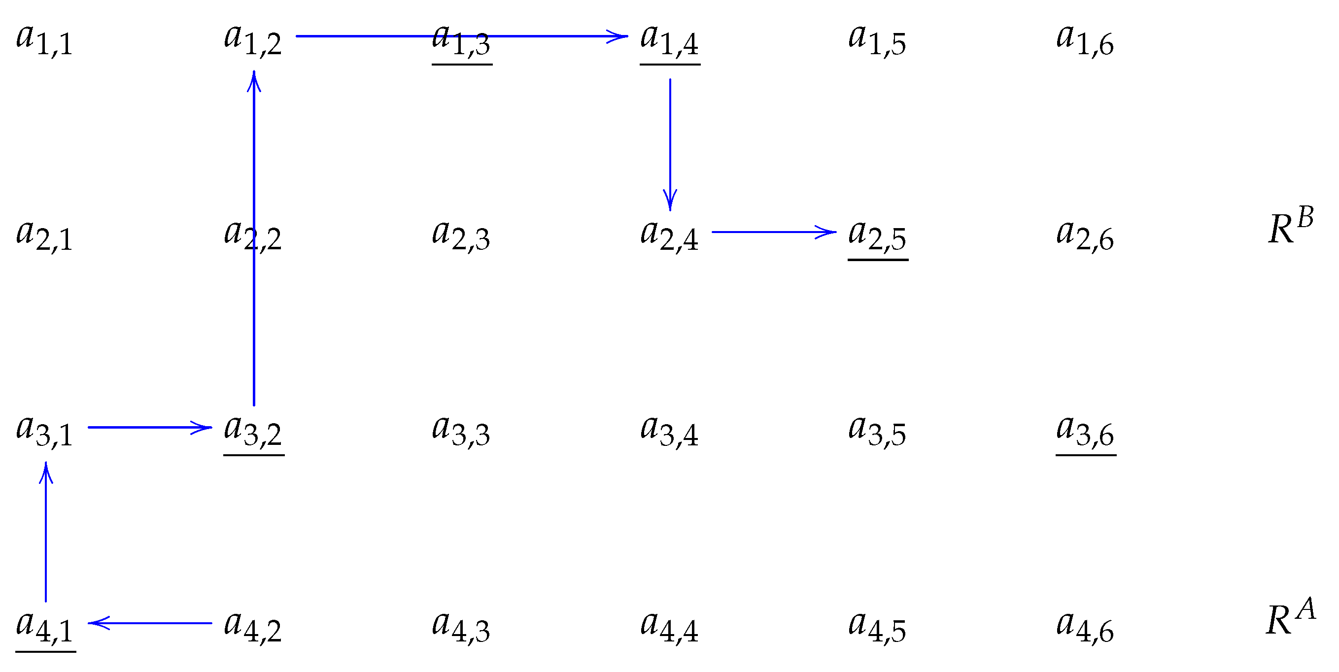
Each non-regular indecomposable Kronecker module has an associated finite set of directed graphs (directed paths) called helices by Espinosa [12]. To construct such graphs, the 1’s in the canonical non-regular Kronecker modules are called pivoting vertices or pivoting entries. Then, the helices are constructed by connecting with horizontal and vertical arrows alternatively two-element sets of entries. For instance, the sets with , , are connected first with a horizontal arrow then with a vertical arrow, and so on. In this case, the entries are pivoting entries and the process (of constructing the helix) ends once the helix has visited all the rows of the matrix M. The reader is referred to [9,12] for a more detailed description of a helix construction.
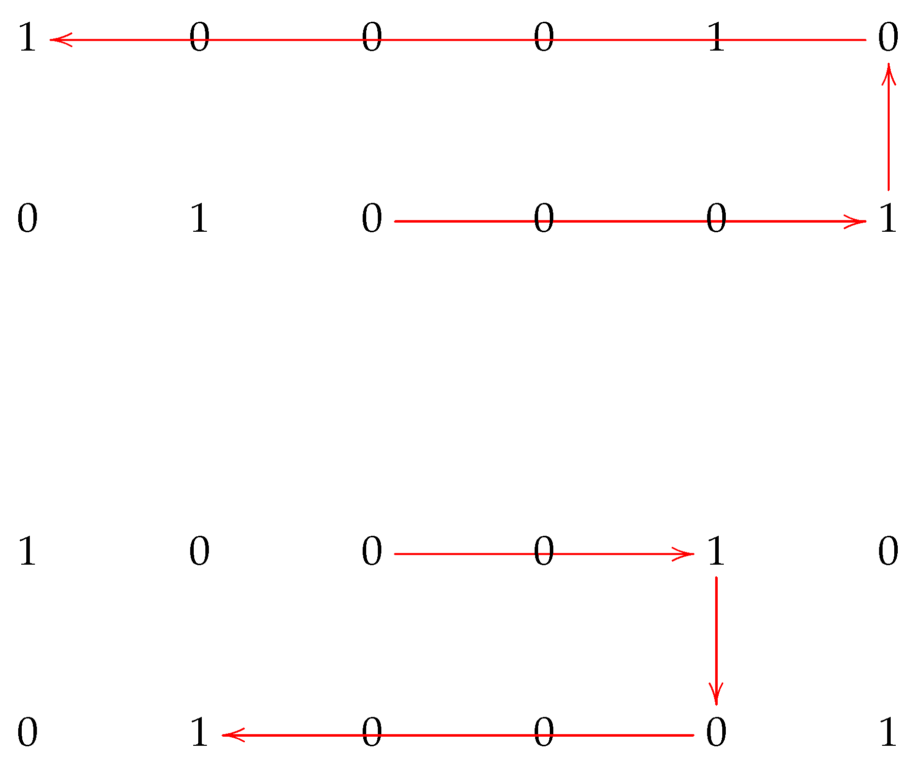
In [9], Espinosa et al. proved that the number of helices associated with the preprojective Kronecker module is , and they used this result to categorize the integer sequence A052558 in the sense of Ringel and Fahr [13,14]. They also noted that each helix is given by a word of the form defined by the way that the helix visits the entries of the matrix M. Figure 4 is an example of a helix given by the word .
Figure 5 shows examples of the helices associated with the indecomposable pre-injective Kronecker module .
Note that each helix defines a snake graph; in such a case, the first horizontal arrow induced a horizontal straight snake graph whose tiles are given by the entries occurring from to , the first vertical straight snake graph is given by the entries from to and so on. Henceforth, we assumed that the helices associated with preprojective and pre-injective Kronecker modules are snake graphs.
4.1. Automatic Sequences and Automatic Categories
A deterministic finite automaton (DFA) [17] is defined as a 5-tuple
where
- Q is a finite set of states;
- is the finite input alphabet;
- is the transition function;
- is the initial state;
- is the set of accepting states.
If the empty word , then for all . Furthermore, for all , , and . It holds that
The language accepted by M is defined in such a way that
A state q of a DFA is said to be reachable if there exists such that , and it is unreachable otherwise [16,17,18].
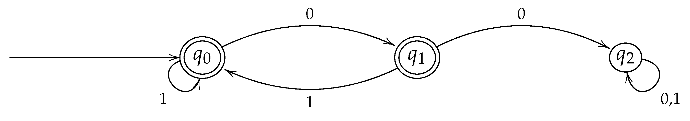
A DFA can be represented by a directed graph, a letter indicates the new state of the machine if the given letter is read. By convention, the initial state is drawn with an unlabeled arrow entering the state, and accepting states are drawn with double circles. For instance, let us consider the automaton for which
- ,
- ,
- , , , , .
- .
The following Figure 6 shows the graphical representation of the automaton , which accepts all strings over that do not contain two consecutive 0s.
4.2. Automatic Sequences
According to Shallit et al. [17], research on automatic sequences dates back to the 1960s with Büchi’s work [34], who attempted to prove that the set of powers of an integer is k-automatic if and only if n and k are multiplicatively dependent. They also reiterate that Cobham [35] was the first to study k-automatic sequences systematically and that Deshouillers coined the term automatic sequence in 1979.
A DFA with output (DFAO) is a DFA M with two additional parameters and , such that is the output alphabet and is the output function. This machine induces a function such that . is said to be a finite-state function.
Note that, if , is a DFAO then the set is a regular language.
A sequence over a finite alphabet is k-automatic if there is a k-DFAO, , such that for all and all w with , i.e., the set and if [17].
Let be integers . Let r be a real number, and suppose that for and . Then, r is said to be -automatic if the sequence of digits is a k-automatic sequence. We let denote the set of all -automatic reals.
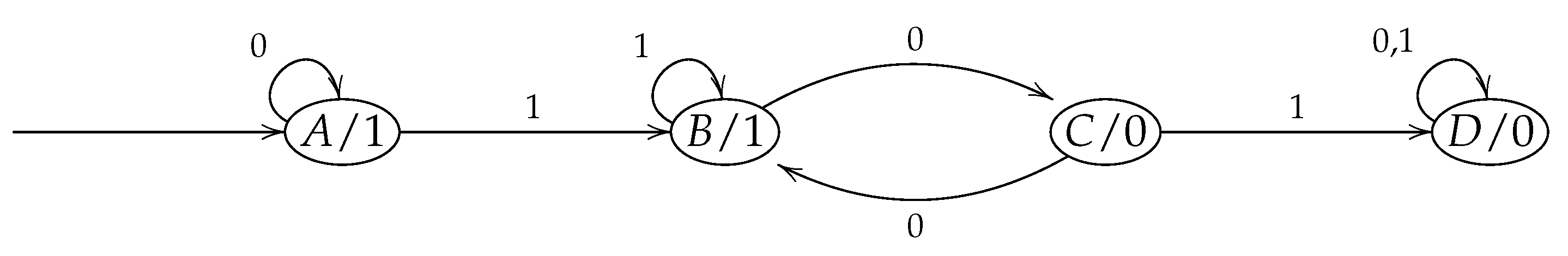
The Baum–Sweet sequence is an example of an automatic sequence (see Figure 7).
The sequence is 2-automatic. It coincides with the sequence of Catalan numbers modulo 4.
A subset is k-automatic if there exists a regular language such that .
The following results regard automatic sequences.
Theorem 2
(Theorem 13.1.1, [17]). If r is a rational number, then ; for all , i.e., r is a -automatic real number.
Theorem 3
(Theorem 13.1.5, [17]). If then .
Corollary 1
(Theorem 13.1.7, [17]). The set constitutes a vector space over the rational numbers.
Theorem 4
(Theorem 14.6.2, [17]). The sequence is k-automatic if and only if the integers d and k are powers of the same prime number p. In this case, the sequence is -automatic for any .
It is worth pointing out that the class of k-automatic sets is closed under union, intersection complement, and set addition.
4.3. Automatic Categories
Let be a Krull–Schmidt category whose indecomposable objects are automatic sets (i.e., they can be obtained as outputs of a DFA or a DFAO), then is said to be an automatic category. Particularly, suppose a k-automatic sequence of real numbers is categorized (in the sense of Ringel and Fahr [13,14]) by the indecomposable objects of the category . In that case, it is said to be an k-automatic category with respect to the sequence . For instance, Rees [19] proved that the string and band modules associated with a monomial algebra are automatic. To do that, she built an automaton that recognizes strings. It is worth pointing out that a unique band is associated with the Kronecker algebra. We recall that a sequence of letters (arrows) associated with a monomial algebra is a string (of length n) if the following conditions hold:
- , for all ;
- , note that , ;
- For all , neither the sequence nor the sequence is contained in I.
A string of length is cyclic if . If additionally, there is no string such that the m-fold concatenation equals . Then, is a primitive cyclic string. If a primitive cyclic string is such that for all and is also an inverse letter whilst is a direct letter, then is a band.
Given a Krull–Schmidt category , a full subcategory L of closed under direct sums and direct summands (and isomorphisms) will be called an object class in [10]. In such a case, L is a Krull–Schmidt category, and is uniquely determined by the indecomposable objects belonging to L. is the smallest object class containing M. is the smallest object classes, comprising as elements.
5. Main Results
This section gives the main results of this paper. Firstly, we prove that, for fixed, the category is automatic. In the last section, we introduce the skew brace induced by the helices associated with pre-injective Kronecker modules.
5.1. Automaticity Associated with Kronecker Modules
The following result proves that preprojective Kronecker modules give rise to automatic categories as a consequence of the Theorems 2—4 and Corollary 1.
Theorem 5.
For fixed, the category is automatic.
Proof.
For , each helix (associated with the preprojective Kronecker module ) starting and ending at the vertices ( and () if n is odd (even)) define a DFA such that
- The set of states Q is given by the entries of the preprojective Kronecker module . We assume that the helix starts in an entry and ends in a vertex , .
- The language .
- The transition function is given by the arrows in the helix . We let () be the corresponding set of vertices (arrows), , and denotes the word associated with the helix such that .
- The initial state .
- The set of final states .
Since, preprojective Kronecker modules can be obtained via the union of helices, which are isomorphic as graphs. □
Note that the automaton defined by the helix shown in Figure 4 is given by the following identities:
- .
- .
- .
- .
Let us now introduce the sequences of continued fractions such that, for fixed and , it holds that , , where the sequences , only consist of 1s and satisfy the following conditions:
- .
- .
- .
- .
Corollary 2.
For and , the sequence is automatic.
Proof.
For and , the fixed continued fraction
gives rise to a snake graph of the form
Vertical straight snake graphs of length 2 appear as transitions of the form .
Now, we fix a preprojective Kronecker module with the form and assume that its entries determine tiles in such a way that the snake graph corresponds to the helix with vertices
; ; ; ; ; ; ; ; , .
Sequence is generated by an automaton such that
- .
- .
- .
- .
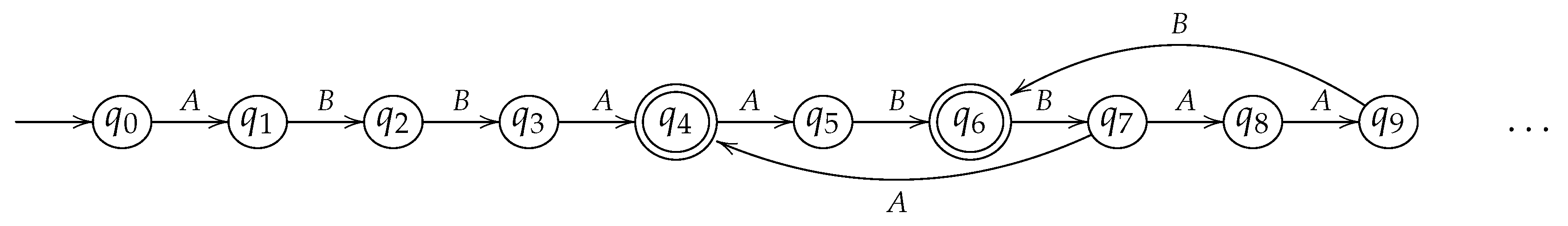
- The transition function is defined in such a way that for , it holds thatIn particular, if or and w does not encode a subpath of a helix associated with the sequence , (Figure 8 shows an example of an automaton that recognizes the sequence ).We note that the automaton recognizes words of the form or of length , . □
Figure 8.
Example of an automaton accepting the terms of the sequence . , , , and so on.

5.2. Skew Braces Associated with Kronecker Modules
The result presented in this section proves that helices associated with pre-injective Kronecker modules give rise to skew braces. In this case, we assume that the matrix form of such modules are given as in identities (8) and (9), i.e., a pre-injective module P can be written as a matrix block , where E and F are matrices.
We let denote the set of helices associated with the pre-injective Kronecker module endowed with an operation ∘ (multiplication). In such a case, each helix can be written in the form:
where starting vertices are entries in the null column of matrix E, the visit all the rows of the indecomposable, , if and .
∘ is defined in such a way that if then
then
with and or equivalently
It is possible to endow with another operation + (addition) by bearing in mind that the map f
defines a bijection between and the symmetric set . Henceforth, we assume that the notation , if .
+ is defined in such a way that, if , then if and with .
The following result proves that helices associated with pre-injective Kronecker modules induce a skew brace, thus constituting a solution of the Yang–Baxter equation according to Lemma 1 and Theorem 1.
Theorem 6.
For fixed, the set of helices endowed with the addition + and multiplication ∘ as defined above is a skew brace.
Proof.
Firstly, we will prove that and are groups. To do that, it suffices to note that, by definition, is closed under addition and multiplication. Since it is easy to see that these operations are associative. We will focus on the description of the corresponding units and inverses.
The identity element is a helix defined in the following fashion:
Note that, where is the identity of the symmetry group . The multiplicative inverse of a helix
is a helix defined in such a way that
where , for all .
On the other hand, provided that
For any with , it holds that
Thus, .
Finally, we note that for all helices with , , for some , it holds that;
Thus, is a skew brace. □
Remark 1.
We note that some details included in the proof of Theorem 6 can be omitted, taking into account that, according to Vendramin et al. [22], groups give rise to skew braces, also called almost trivial skew braces by Koch et al. [36]. However, for the sake of clarity, we prove that satisfies all the properties that make it a skew brace.
5.3. Discussion
This paper provides new applications of the non-regular modules over the Kronecker algebra. On the one hand, snake graphs associated with preprojective Kronecker modules allow proving the automaticity of some continued fraction sequences. On the other hand, snake graphs associated with pre-injective Kronecker modules give rise to particular classes of skew braces that define the set-theoretical solutions of the Yang–Baxter equation (see Lemma 1 and Theorem 1).
As an example, the following are the elements of , where denotes the helix associated with the permutation , denoted ;
Some products
The Cayley table of appears as follows:
| ∘ | ||||||
The Cayley table of has the following shape:
| + | ||||||
6. Concluding Remarks
This paper explored new interactions between the representation theory of the Kronecker algebra and studies dealing with the Yang–Baxter equation and automatic sequences. On the one hand, it is proven that preprojective Kronecker modules are automatic in the sense that a suitable automaton generates them. Actually, it is possible to conclude that Krull–Schmidt categories generated by a finite number of preprojective Kronecker modules are automatic. This result is obtained provided that any non-regular module over the Kronecker algebra has an associated set of snake graphs, as such snake graphs allow one to prove that some sequences of continued fractions are also automatic.
On the other hand, it is proven that the snake graphs associated with pre-injective Kronecker modules give rise to the solutions of the Yang–Baxter equation. To do that, such a set of snake graphs is endowed with two non-commutative operations, making it a skew brace.
Future Work
The following are interesting tasks to carry out in the future.
- To define automatic sequences based on invariants of indecomposable modules of different Krull–Schmidt categories.
- To determine the braces via solutions of generalized matrix problems.
Author Contributions
Investigation, writing, review and editing, A.M.C., P.F.F.E., and A.B.-B. All authors have read and agreed to the published version of the manuscript.
Funding
Seminar Alexander Zavadskij on Representation of Algebras and their Applications, Universidad Nacional de Colombia.
Institutional Review Board Statement
Not applicable.
Informed Consent Statement
Not applicable.
Data Availability Statement
Not applicable.
Conflicts of Interest
The authors declare no conflict of interest.
Abbreviations
The following abbreviations are used in this manuscript:
| (Category generated by objects ) | |
| (Continued fraction) | |
| DFA | (Deterministic finite automaton) |
| (Empty word) | |
| (Field) | |
| (Language associated with an automaton) | |
| (Preprojective Kronecker module) | |
| (Preinjective Kronecker module) | |
| (Set of helices associated with a pre-injective Kronecker module) | |
| (Snake graph) | |
| YBE | (Yang–Baxter equation) |
References
- Yang, C.N. Some exact results for the many-body problem in one dimension with repulsive delta-function interaction. Phys. Rev. Lett. 1967, 19, 1312–1315. [Google Scholar] [CrossRef]
- Baxter, R.J. Partition function for the eight-vertex lattice model. Ann. Phys. 1972, 70, 193–228. [Google Scholar] [CrossRef]
- Aragona, R.; Civino, R.; Gavioli, N.; Scoppola, C.M. Regular subgroups with large intersection. Ann. Mat. Pura Appl. 2018, 198, 2043–2057. [Google Scholar] [CrossRef] [Green Version]
- Chen, R. Generalized Yang-Baxter equations and braiding quantum gates. J. Knot Theory Ramif. 2012, 21, 1250087. [Google Scholar] [CrossRef] [Green Version]
- Kauffman, L.H.; Lomonaco, S.J. Braiding operators are universal quantum gates. New J. Phys. 2004, 6, 134. [Google Scholar] [CrossRef]
- Nichita, F.F. Introduction to the Yang-Baxter equation with open problems. Axioms 2012, 1, 33–37. [Google Scholar] [CrossRef] [Green Version]
- Nichita, F.F. Yang-Baxter equations, computational methods and applications. Axioms 2015, 4, 423–435. [Google Scholar] [CrossRef] [Green Version]
- Massuyeau, G.; Nichita, F.F. Yang-Baxter operators arising from algebra structures and the Alexander polynomial of knots. Commun. Algebra 2005, 33, 2375–2385. [Google Scholar] [CrossRef] [Green Version]
- Agudelo, N.; Cañadas, A.M.; Espinosa, P.F.F. Brauer configuration algebras defined by snake graphs and Kronecker modules. Electron. Res. Arch. 2022, 30, 3087–3110. [Google Scholar]
- Simson, D. Linear Representations of Partially Ordered Sets and Vector Space Categories; Gordon and Breach: London, UK, 1992. [Google Scholar]
- Zavadskij, A.G. On the Kronecker problem and related problems of linear algebra. Linear Algebra Appl. 2007, 425, 26–62. [Google Scholar] [CrossRef] [Green Version]
- Espinosa, P.F.F. Categorification of Some Integer Sequences and Its Applications. Ph.D. Thesis, Universidad Nacional de Colombia, Bogotá, Colombia, 2021. [Google Scholar]
- Fahr, P.; Ringel, C.M. Categorification of the Fibonacci numbers using representations of quivers. J. Integer Seq. 2008, 11, 12.2.1. [Google Scholar]
- Fahr, P.; Ringel, C.M. A partition formula for Fibonacci numbers. J. Integer Seq. 2012, 15, 08.14. [Google Scholar]
- Turing, A.M. On computable numbers with an application to the Entscheidungs problem. Proc. Lond. Math. Soc. 1937, 42, 230–265, Corrigendum in Proc. Lond. Math. Soc. 1937, 43, 544–546. [Google Scholar] [CrossRef]
- Shallit, J.O. Number theory and formal languages. In Emerging Applications of Number Theory, IMA; Springer: Berlin/Heidelberg, Germany, 1999; pp. 547–570. [Google Scholar]
- Allouche, J.-P.; Shallit, J.O. Automatic Sequences: Theory, Applications, Generalizations; Cambridge University Press: Cambridge UK, 2003. [Google Scholar]
- Adamczewski, B.; Cassaigne, J. Diophantine properties of real numbers generated by finite automata. Compos. Math. 2006, 142, 1351–1372. [Google Scholar] [CrossRef] [Green Version]
- Rees, S. The automata that define representations of monomial algebras. Algebr. Represent. Theory 2008, 11, 207–214. [Google Scholar] [CrossRef]
- Rye, A.-B. The 2-Kronecker Quiver and Systems of Linear Differential Equations. Master’s Thesis, Norwegian University of Science and Technology (NTNU), Trondheim, Norway, 2013. [Google Scholar]
- Feinsilver, P.; Kocik, J. Krawtchouk Polynomials and Krawtchouk Matrices. In Recent Advances in Applied Probability; Baeza-Yates, R., Glaz, J., Gzyl, H., Hüsler, J., Palacios, J.L., Eds.; Springer: Boston, MA, USA, 2005; pp. 115–141. [Google Scholar]
- Guarnieri, L.; Vendramin, L. Skew braces and the Yang-Baxter equation. Math. Comput. 2017, 85, 2519–2534. [Google Scholar] [CrossRef]
- Cedó, F.; Jespers, E.; Okniński, J. Braces and the Yang-Baxter equation. Commun. Math. Phys. 2014, 327, 101–116. [Google Scholar] [CrossRef] [Green Version]
- Cedó, F.; Jespers, E.; Okniński, J. Set-theoretical solutions of the Yang-Baxter equation, associated quadratic algebras and the minimality condition. Rev. Mat. Complut. 2020, 34, 99–129. [Google Scholar] [CrossRef] [Green Version]
- Rump, W. Modules over braces. Algebra Discret. Math. 2006, 2, 127–137. [Google Scholar]
- Rump, W. Braces, radical rings, and the quantum Yang-Baxter equation. J. Algebra 2007, 307, 153–170. [Google Scholar] [CrossRef] [Green Version]
- Ballester-Bolinches, A.; Esteban-Romero, R.; Fuster-Corral, N.; Meng, H. The structure group and the permutation group of a set-theoretical solution of the quantum Yang-Baxter equation. Mediterr. J. Math. 2021, 18, 1347–1364. [Google Scholar] [CrossRef]
- Drinfeld, V.G. On unsolved problems in quantum group theory. Lect. Notes Math. 1992, 1510, 1–8. [Google Scholar]
- Etingof, P.; Schedler, T.; Soloviev, A. Set-theoretical solutions to the quantum Yang-Baxter equation. Duke Math. J. 1999, 100, 169–209. [Google Scholar] [CrossRef] [Green Version]
- Gateva-Ivanova, T.; Van den Bergh, M. Semigroups of I-type. J. Algebra 1998, 308, 97–112. [Google Scholar] [CrossRef] [Green Version]
- Çanackçi, I.; Schiffler, R. Snake graphs calculus and cluster algebras from surfaces. J. Algebra 2013, 382, 240–281. [Google Scholar] [CrossRef]
- Çanackçi, I.; Schiffler, R. Cluster algebras and continued fractions. Compos. Math. 2018, 154, 565–593. [Google Scholar] [CrossRef] [Green Version]
- Çanackçi, I.; Schiffler, R. Snake graphs and continued fractions. Eur. J. Comb. 2020, 86, 103081. [Google Scholar] [CrossRef] [Green Version]
- Büchi, J.R. Weak secord-order arithmetic and finite automata. Z. Math. Log. Grundl. Math. 1960, 6, 66–92, Reprinted in The Collected Works of J. Richard Büchi; Lane, S.M., Siefkes, D., Eds.; Springer: New York, NY, USA, 1990; pp. 398–424. [Google Scholar] [CrossRef]
- Cobham, A. Uniform tag sequences. Math. Syst. Theory 1972, 6, 164–192. [Google Scholar] [CrossRef]
- Koch, A.; Truman, P.J. Opposite skew left braces and applications. J. Algebra 2020, 546, 218–235. [Google Scholar] [CrossRef] [Green Version]
Figure 2.
Snake graph of type .

Figure 3.
A sequence associated with the snake graph .

Figure 4.
Helix defined by the word . Numbers denote the pivoting entries.

Figure 5.
Helices associated with the pre-injective Kronecker module .

Figure 6.
Example of an automaton.

Figure 7.
2-DFAO generating the Baum–Sweet sequence. X/j means that the output associated with the state X is j [17].
Figure 7.
2-DFAO generating the Baum–Sweet sequence. X/j means that the output associated with the state X is j [17].

Disclaimer/Publisher’s Note: The statements, opinions and data contained in all publications are solely those of the individual author(s) and contributor(s) and not of MDPI and/or the editor(s). MDPI and/or the editor(s) disclaim responsibility for any injury to people or property resulting from any ideas, methods, instructions or products referred to in the content. |
© 2023 by the authors. Licensee MDPI, Basel, Switzerland. This article is an open access article distributed under the terms and conditions of the Creative Commons Attribution (CC BY) license (https://creativecommons.org/licenses/by/4.0/).
Share and Cite
MDPI and ACS Style
Cañadas, A.M.; Fernández Espinosa, P.F.; Ballester-Bolinches, A. Solutions of the Yang–Baxter Equation and Automaticity Related to Kronecker Modules. Computation 2023, 11, 43. https://doi.org/10.3390/computation11030043
AMA Style
Cañadas AM, Fernández Espinosa PF, Ballester-Bolinches A. Solutions of the Yang–Baxter Equation and Automaticity Related to Kronecker Modules. Computation. 2023; 11(3):43. https://doi.org/10.3390/computation11030043
Chicago/Turabian StyleCañadas, Agustín Moreno, Pedro Fernando Fernández Espinosa, and Adolfo Ballester-Bolinches. 2023. "Solutions of the Yang–Baxter Equation and Automaticity Related to Kronecker Modules" Computation 11, no. 3: 43. https://doi.org/10.3390/computation11030043
Note that from the first issue of 2016, this journal uses article numbers instead of page numbers. See further details here.