Article

Irradiance Non-Uniformity in LED Light Simulators

by
Vasiliki Naskari
*,
Gregory Doumenis
and
Ioannis Masklavanos
Department of Informatics and Telecommunications, University of Ioannina, GR47100 Arta, Greece
*
Author to whom correspondence should be addressed.
Information 2023, 14(6), 316; https://doi.org/10.3390/info14060316
Submission received: 6 April 2023 / Revised: 26 May 2023 / Accepted: 26 May 2023 / Published: 30 May 2023

Abstract

:
Photovoltaic (PV) cells are a technology of choice for providing power to self-sufficient Internet of Things (IoT) devices. These devices’ declining power demands can now be met even in indoor environments with low light intensity. Correspondingly, light simulation systems need to cover a wide spectrum of irradiance intensity to emulate a PV cell’s working conditions while meeting cost targets. In this paper, we propose a method for calculating the irradiance distribution for a given number and position of LED sources to meet irradiance and uniformity requirements in LED-based light simulators. In addition, we establish design guidelines for minimizing non-uniformity under specific constraints and utilize a function to evaluate the degree of non-uniformity and determine the optimal distance from the illuminated surface. We demonstrate that even with a small number of low-cost LED sources, high levels of irradiance can be achieved with bounded non-uniformities. The presented guidelines serve as a resource for designing tailored, low-cost light simulators that meet users’ area/intensity/uniformity specifications.

1. Introduction

The rapid expansion of industrialization, coupled with population growth and an increase in energy consumption per capita, has resulted in a surge in energy demand across the globe. However, the use of fossil fuels for energy production has reached saturation levels due to escalating environmental concerns and resource depletion [1]. To address this challenge, the focus has turned toward more economical, cost-effective, and environmentally friendly energy solutions, with renewable energy sources (RESs) being the most promising solution to meet the growing energy demand [2].
At the same time, the Internet of Things (IoT) has become an integral part of modern society, enabling the connectivity of physical devices through the internet and introducing new forms of communication between people and things, as well as between things themselves [3]. Through the exchange of data for remote monitoring and controlling devices, the IoT has become an essential technology in daily life around the world [4,5,6].
Solar energy is a clean and renewable source of energy, which makes it an attractive option for powering IoT nodes, especially those located in remote or inaccessible areas where it is difficult or expensive to run power lines. Solar-powered IoT nodes can be used for various applications, such as environmental monitoring, smart agriculture, and industrial automation, among others. Furthermore, advancements in solar technology have enabled the use of solar power to provide energy to small, low-power devices that consume very little energy, such as sensors and actuators. These devices can collect data and perform automated actions without the need for human intervention, thereby improving the efficiency and sustainability of energy consumption and reducing the overall carbon footprint of IoT networks [7,8].
Photovoltaic cells have been extensively studied and have resulted in high conversion efficiencies of up to 20% in optimal weather conditions [8]. However, research on the performance of photovoltaic cells under indoor lighting conditions is much less efficient than that under sunlight. The demand for an accurate description of these specialized photovoltaic cells has increased in recent years due to the growing interest in using indoor light as a power source for ultra-low-power Internet of Things devices [9].
The lack of information on the performance of indoor photovoltaic cells under low light conditions is a concern. It is not possible to guarantee their efficiency and reliability because their performance characteristics at lower light irradiances have not been defined. Datasheets for these cells often only provide information on their efficiency at high irradiance levels, which leads to differences between the values indicated on the datasheets and the final measured values, which can vary significantly when evaluating an indoor solar cell.
As shown in Figure 1, when evaluating MP3-37, the manufacturer provides I/V curves for both the conventional 1-sun and 1/4-sun irradiance [10]. Figure 2 illustrates a significant drop in power output at low irradiance levels. This information is crucial for determining the feasibility of using indoor PV cells for a specific application, as well as for optimizing their performance in low-light conditions. Therefore, there is a need for more comprehensive testing and reporting of indoor PV cell performance to ensure an accurate and reliable product evaluation.
To address the issue of the lack of detailed information on the performance of indoor PV cells under low-light conditions, light simulators are often used to evaluate such devices. Light simulators allow the precise control of the intensity, spectrum, and direction of the light source, which can be used to simulate a wide range of indoor lighting conditions. By testing PV cells under a variety of simulated lighting conditions, researchers and manufacturers can better understand the performance of these devices and provide more accurate efficiency ratings for different lighting conditions. Light simulators can also be used to optimize the design of indoor PV cells for specific indoor lighting conditions and to identify opportunities for improving the efficiency and performance of these devices [11]. However, these devices are expensive and bulky. The greatest drawback of these devices is their inability to uniformly illuminate a larger surface [12]. Increasing uniformity can be achieved by increasing the number of light sources or by sacrificing illuminance. Our method achieves the appropriate tradeoff of illumination/non-uniformity and minimizes the cost (due to a reduced amount of LEDs). Our work focuses on solving the PV validation problem from the perspective of desired illumination and non-uniformity. Other factors, such as spectral distribution, are not considered in the current work.

1.1. Related Work

Several studies have focused on the development of light simulator systems for various applications, such as photovoltaic (PV) cell testing and research, education, and indoor use. Many of these systems have aimed to reach a solar intensity of 1 sun, which is the standard measurement used to determine the output of PV cells under real sunlight conditions. However, some of these systems have sacrificed either the uniformity of the irradiance distribution or the cost resulting from the use of a large number of light-emitting diodes (LEDs).
One such system, developed by Lopez-Fraguas et al. [13], is a low-cost simulator that achieves sufficient uniformity to be classified as Class AAA in a 1 cm2 central area using a 34 LED array. Moria [14] developed a solar simulator using 8 500 W halogen lamps, which achieved high irradiance values between 500 and 1100 W/m2 for research and education purposes. Irwan et al. [15] constructed and fabricated a solar simulator system using 20 Philips halogen 500 W lamp bulbs. Elgendy et al. [16] developed 2 maximum power point tracking (MPPT) algorithms for PV arrays and verified them by fabricating a 40 Wp PV generator for indoor use by switching 60 low-cost halogen lamps. Landrock et al. [17] constructed a low-cost solar simulator using an array of 6 halogen spotlight bulbs (AC 50 W/120 V Halogena; General Electric) to improve tungsten light source systems for PV cell testing. Finally, Yandri et al. [18] developed a simple, low-cost, compact halogen solar simulator that consisted of 16 halogen lamps (50 W/110 V).
The utilization of solar simulators extends beyond their exclusive application in research endeavors. In recent years, there has been a noteworthy upsurge in the production of solar simulators tailored for commercial purposes. This burgeoning trend arises from the recognition of solar energy as a viable and sustainable alternative to conventional power sources, prompting industries to invest in technologies that facilitate the efficient testing and evaluation of solar devices. In Table 1, a few commercial solar simulators are presented as indicative examples that have been built to meet the diverse needs of the solar industry.
In summary, studies and industries have developed solar simulator systems using a variety of methods and light sources to achieve a 1-sun intensity for different applications. The systems vary in terms of cost, uniformity, and irradiance values, and each has its own unique advantages and limitations.

1.2. Problem Statement

Achieving maximum uniformity in an indoor photovoltaic (PV) rating system is of paramount importance for several reasons. Firstly, a uniform irradiance distribution across an entire PV panel surface ensures that each cell within the panel receives the same amount of irradiance, thereby maximizing the overall energy output of the system. This is especially crucial in indoor environments, where the available irradiance is typically lower than in outdoor environments, and any non-uniformity in the irradiance distribution can significantly impact the energy generation potential of the PV panel [19].
Furthermore, uniformity in the irradiance distribution is crucial for the accurate performance evaluation and comparison of different PV panels. In a rating system, the energy output of a PV panel is typically compared with its rated capacity, which assumes a uniform irradiance distribution. Any non-uniformity in the irradiance distribution can lead to inaccurate performance measurements, making it challenging to compare the energy output of different panels and assess their overall performance.
Due to all these factors, achieving the minimization of non-uniformity is one of the main interests in this work.

2. Methods for Irradiance Pattern Modeling of LED Sources

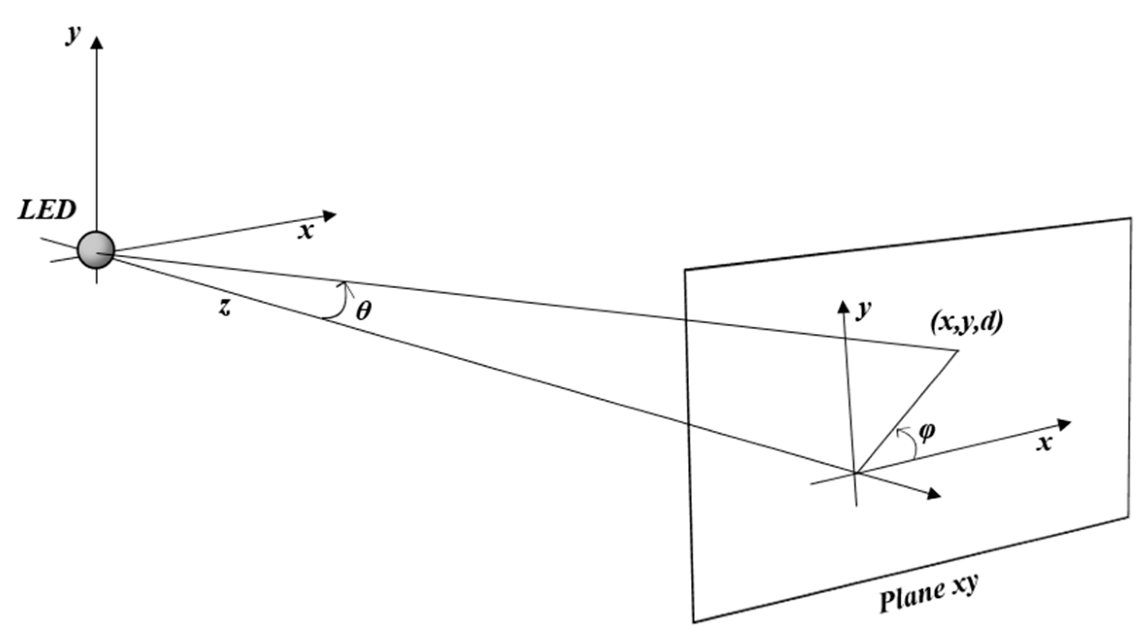
2.1. Modeling of Multisource Irradiance on a Plane

Our team was engaged in the (progressive) development of an economical artificial light simulation system that was specifically designed for the experimental verification of small-sized PV cells. The system should be able to adapt to a PV cell’s area and regulate the light intensity at the PV cell surface within a given range while keeping any non-uniformity at acceptable levels.
After considering various options, we opted to use LEDs as our light sources due to their widespread availability, their low cost, and the ease of regulating their intensity. Additionally, LEDs offer diverse spectral emissions, making it possible to simulate different artificial light sources by blending multiple LEDs.
In our study, we assumed that there was no optical diffusion added (with optical diffusers) and that irradiance variation from a point source was approximately described using the inverse-square law. Furthermore, we modeled each LED source as an imperfect Lambertian emitter.
To minimize any interference, we proposed an enclosed design, which does not have to be entirely reflection-free. In this design, the PV cell is attached (face up) to a horizontal plane (the illuminated surface), while the LED source(s) are attached (face down) to an opposing flat surface (the illumination head). The number of LEDs and their placements on the illumination head are significant parameters of our design. The distance between the two surfaces (the height) can be adjusted to provide additional control (and tradeoff) of the irradiance intensity and covered area (given that the covered area is proportional to the squared height and, as described in (1),the irradiance intensity is inversely proportional to the squared height).
Our modeling approach begins with a single centrally located LED source and aims to calculate the irradiance and uniformity on the illuminated surface, taking into account the LED’s design parameters and selecting the appropriate drive current to achieve the desired irradiance. If the irradiance, area coverage, and uniformity targets cannot be met with a single LED, we add more LEDs. Their number and topology are adjustable parameters in our model, and we select the lowest-cost topology that meets the set targets for intensity, area coverage, and uniformity.

2.2. Single-Source Irradiance

As shown in Figure 3, without loss of generality, we set the position of an LED at the point of intersection of the x, y, and z axes.
Assuming the polar angle to be θ and the azimuthal angle to be φ, we can mathematically express the radiant flux per solid angle (measured in units of W × sr-1) in a specific direction from the source. This quantity is defined as the intensity, which is denoted as I (θ, φ) and represents the radiant power per unit solid angle and can be obtained by summing the Gaussian functions or cosine-power functions. According to the inverse-square Law, the radiant flux that is incident on a surface per unit area, also known as the irradiance (in units of W × m−2), decreases proportionally to the square of the distance from the source. As light propagates outward from the light source, it spreads out over a larger area. Consequently, the radiant energy becomes more diluted, resulting in a decrease in the irradiance with an increasing distance. By considering this law, the irradiance (Ee) can be mathematically represented as [20]
E e d ,   θ ,   φ = cos m θ   ×   I   θ ,   φ d 2
where d is the distance between the irradiated surface and the light source, and m is a constant value that depends in the relative position of the LED emitting region and is given using the following formula:
m = ln 2 ln ( cos θ 1 2 )
Upon converting the coordinates from the spherical to the rectangular coordinate system and applying the same procedure while altering the location of the LED from (0, 0, 0) to (X, Y, 0), the following expression is obtained [21]:
E e x ,   y ,   z = z m I   θ x ,   y ,   z ,   φ   x ,   y ,   z x X 2 + y Y 2 + z 2 m + 2 2

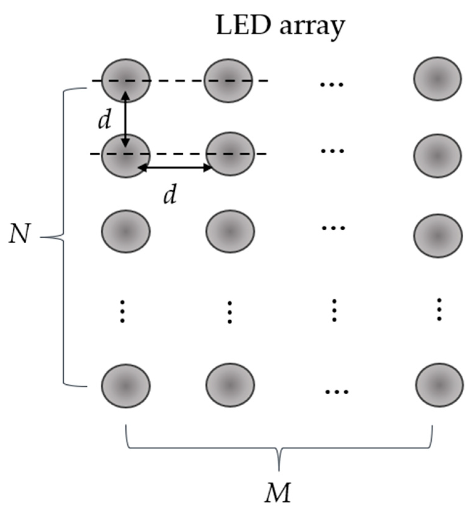
2.3. Multi-Source Irradiance

As previously noted, the distribution of irradiance stemming from a light source can be accurately represented by the summation of multiple Gaussian distributions. Therefore, when referring to a configuration of light sources, according to the principle of superposition, the irradiance at any point on the illuminated surface can be computed based on the summation of the irradiance received from each light source.
The current investigation involved an analysis of geometric LED placements with the aim of augmenting the uniformity of illumination while simultaneously elevating the maximum irradiance values. Previous study which was focused on evaluating several LED array topologies [22], including two-LED, linear, circular, square, triangular, and other arrays showed that the most efficient LED array topology was the square one. Thus, in this study special emphasis was placed on the square LED array configuration.
In the specific case of the square LED array configuration, a graphical representation can be constructed to visually illustrate this arrangement (Figure 4). The utilization of this configuration allows the evaluation of various parameters, including the number of LEDs needed to achieve the desired illumination, the distance between the LEDs, and the angle at which light emanates from each LED.
The irradiance Ee can be calculated as the summation of the irradiances of a matrix of N × M LEDs, as depicted in the following equation [23].
E e x ,   y ,   z = z m I θ x ,   y ,   z ,   φ   x ,   y ,   z i = 1 N j = 1 M x N + 1 2 i d / 2 2 + y M + 1 2 j d / 2 2 + z 2 m + 2 2
where d is the distance between the LEDs.

2.4. Multi-LED Light Simulator Design Guidelines

This work aimed to establish design guidelines that can be employed to minimize non-uniformity to the greatest extent possible, given a specific topology, height between surfaces, the available number of LEDs, and other potential constraints. As we were dealing with equations that involve several parameters, it was necessary to stabilize certain variables to approximate the solution to the problem at hand.
The process began by examining the irradiance along a randomly selected testing plane, assuming that the irradiance distribution could be calculated from a formula of the form Ee (x, y, z), where x and y represent the dimensions of the testing plane, and x ∈ [α, β] and y ∈ [γ, δ]. By analyzing the irradiance distribution for a given z, we obtained a matrix of x × y values, all of which were strictly positive. Thus, we considered the metric space (ℝ, E), where E: ℝ × ℝ → [0, +∞).
The most critical value that we must evaluate is the degree of non-uniformity, which for a two-dimensional space, ℝ2, is described with a single value belonging to the interval [0, 1] [22].
Critical   Value = sup x α , β y γ , δ E e x , y inf x α , β y γ , δ E e x , y sup x α , β y γ , δ E e x , y + inf x α , β y γ , δ E e x , y
In the current study, the procedure under consideration took place in a three-dimensional space, ℝ3. Given a fixed topology of the light sources, by changing only the distance z from the radiated surface, we can observe the change in the non-uniformity on the test plane. This results in the export of the function that describes the non-uniformity relative to the distance from the light source(s).
We observed that there exists an interval subset of the domain of the function critical value, [z1, z2], within which the function varies monotonically. This interval defines a set of optimal distances at which to place the illuminated surface from the surface where the light sources are arranged. Within this interval, we deliberately select a specific value, denoted as z0, in accordance with the predefined criteria pertinent to the problem at hand. For instance, if our objective is to emphasize maximum radiation, we opt for a z0 that is in closer proximity to z1.
Thus, we calculate the height(s) that provide both the targeted coverage and the necessary uniformity levels. Selecting the minimum height enables the surface to be radiated with maximum irradiance or, for a given irradiance requirement, minimizes the power consumption of the LED sources.
The findings are presented using 2D and 3D graphs. Interestingly, the arrangement that generated the greatest interest is the simplest (the square arrangement).

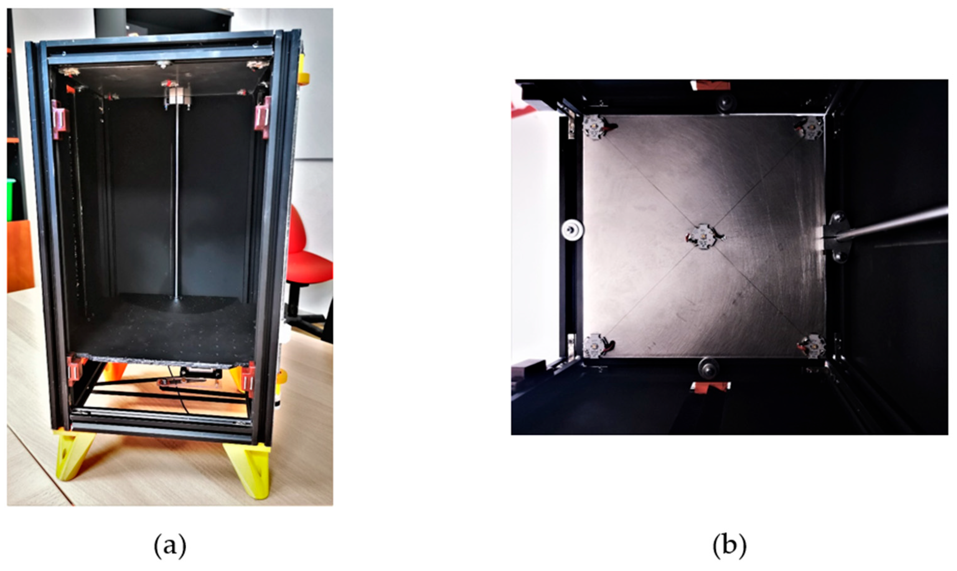
3. Experimental Implementation

3.1. Design of the Low-Cost Light Simulator Used

In this work, a device for evaluating indoor photovoltaic cells was used [24]. This device is equipped with a movable bed that can be adjusted to different heights ranging from 5 to 31 cm relative to the surface where the LEDs are situated, as depicted in Figure 5a. Furthermore, the device features a versatile design that can accommodate various array geometries, owing to the separate power supply of each LED. Specifically, this device can support from a single LED up to five LED light sources, as shown in Figure 5b.
Additionally, the bed was enclosed to mitigate the impact of external light interference, thereby blocking incoming light from the environment. Both the dimensions of the surface on which the LEDs were mounted and the illuminated area measured 18 × 18 cm. As for the light source, we used the low-cost LST1–01G03–4095–01 LED from Luminus [25], which can be purchased for as low as USD 3.7 per unit in large quantities (price sampled from Mouser on 20 May 2023).
To evaluate the experimental device’s performance, we conducted illuminance measurements (since there is no universally recognized standardized reporting condition (SRC) for indoor photovoltaic measurements or calibrated reference cells for low-light measurements). Many researchers rely on illumination meters to measure irradiance and report their findings in units of lux (lx = lm/m2) [26,27]. For our assessment, we utilized the commercially available E-SUN LX-101 instrument, which has a measurement range spanning from 1 up to 50,000 Lux and an accuracy level of ± 5%.

3.2. The Software Model

Previous work by the authors of this study [22] aimed to develop algorithms that are capable of calculating important quantities such as intensity, irradiance, and illuminance. The algorithms were also designed to determine the optimal arrangement of LEDs for a given number of LEDs, the dimensions of the surface, the dimensions of the luminous surface, and the distance between them, all of which are based on the uniformity.
The primary goal of this work was to find a technique for illuminating an area with the lowest possible number of sources.
The experimental measurements were represented and interpreted. In cases where multiple arrangements with similar uniformity were present, preference was given to the arrangement with the smallest number of LEDs, prioritizing cost. Restrictions on uniformity and maximum or minimum irradiance were also considered, and an algorithm extracted the corresponding result. If none of the defined assumptions were satisfied by any of the array configurations, the algorithm would extract the closest result based on the requirements. All algorithms were developed in the MATLAB environment [21].
In addition, an algorithm was developed that calculates the irradiance distribution over a test plane, as well as an interval for the height between the surfaces. This algorithm also extracts the turning point, which is the key factor for this specific case, as well as an analytical graphical representation of the critical value function (z).
Curve fitting, which is a widely used mathematical process in different scientific and technological fields, was used to approximate the irradiance distribution of both the single LED and its adaptation to the square arrangement using the Curve Fitting Tool from MATLAB.

4. Discussion

4.1. Evaluation

One of the most fundamental considerations in the design and development of an application utilizing light-emitting diodes (LEDs) is the efficient and effective distribution of light toward the target area. The optimal method of light distribution is essential for ensuring the desired functionality and overall effectiveness of the application. Therefore, careful evaluation of the light distribution is crucial in both the design and development stages of the application.
To this end, various methods of evaluating the results of the light distribution are utilized. These methods may include measuring intensity, irradiance, and illuminance, among other pertinent properties. The interpretation of such results can then provide valuable insight into the efficacy of the light distribution method and inform potential modifications or improvements of the application design.

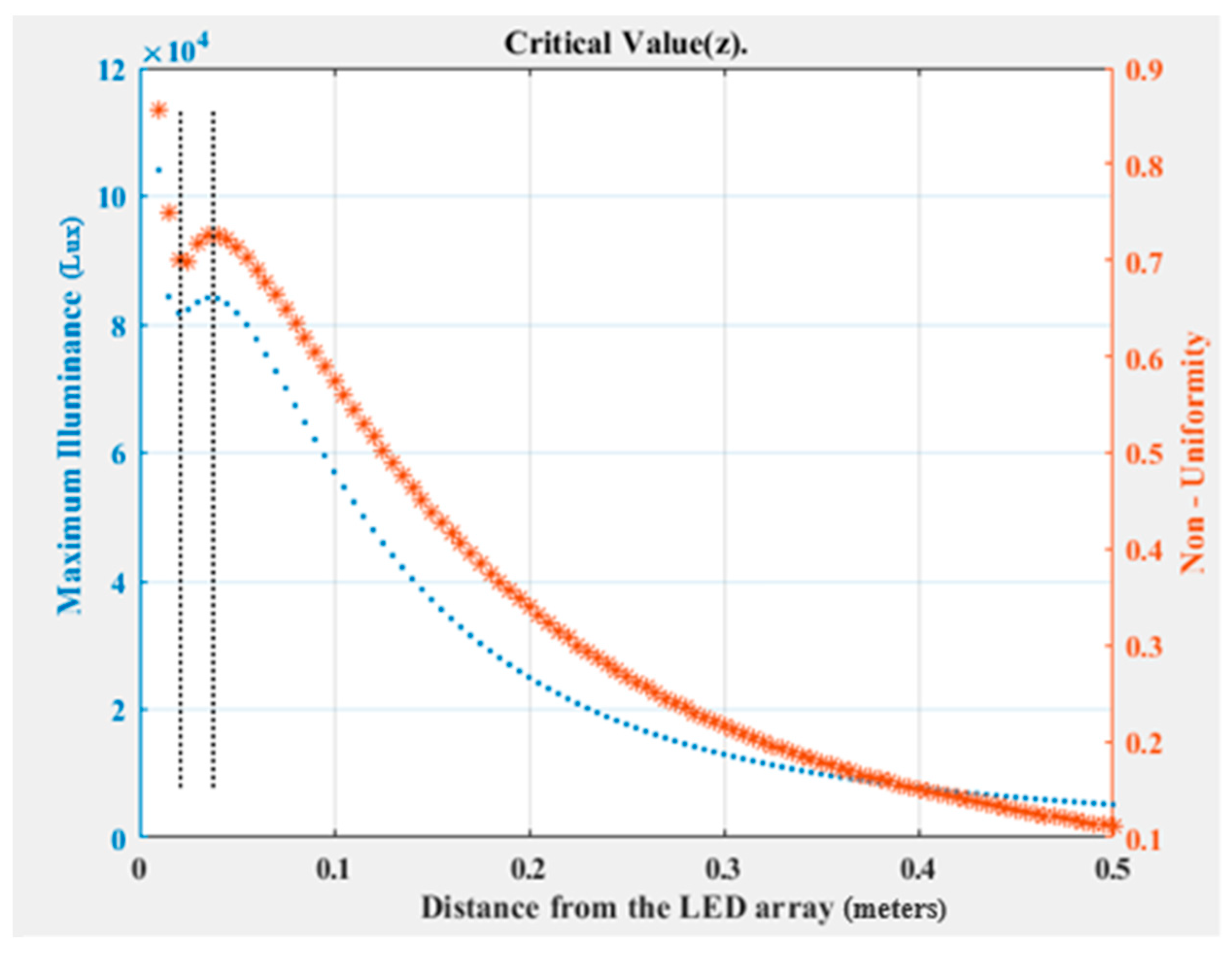
4.1.1. Uniformity of Illumination Distribution

The illumination of a given area is determined by the applied lighting, in accordance with the prescribed criteria for light uniformity. When evaluating the uniformity of illumination, the commonly used metric is the ratio of the minimum illumination to the maximum illumination across the area of interest. The degree of uniformity is determined using a formula that quantifies the ratio of the minimum illumination to the average illumination across the area of interest [28].
U 1 = E v m i n E v average  
U 2 = E v m i n E v max
where U and Ev stand for the uniformity and illuminance, respectively.

4.1.2. Non-Uniformity

Irradiance non-uniformity is a critical parameter that characterizes the degree of deviation from uniformity in the irradiance distribution across an entire test plane. It represents the maximum relative error between the measured irradiance values and their ideal, uniform distribution and can be mathematically expressed as [29]
Non - Uniformity = E e max     E e min E e max + E e min   ×   100 %
where Eemax and Eemin are the maximum and the minimum values of irradiance [W/m2] across the entire test plane.

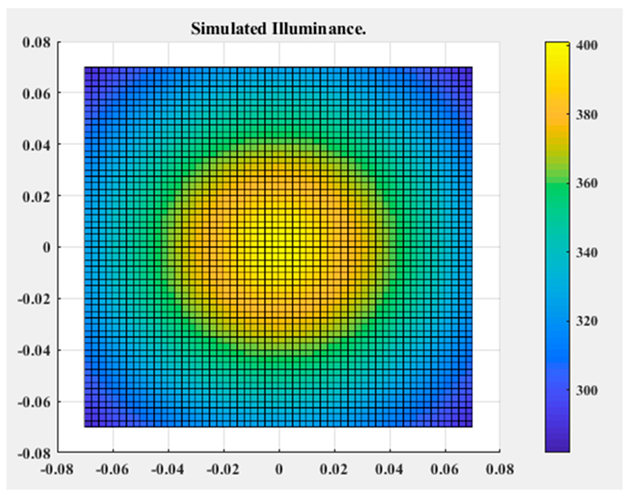
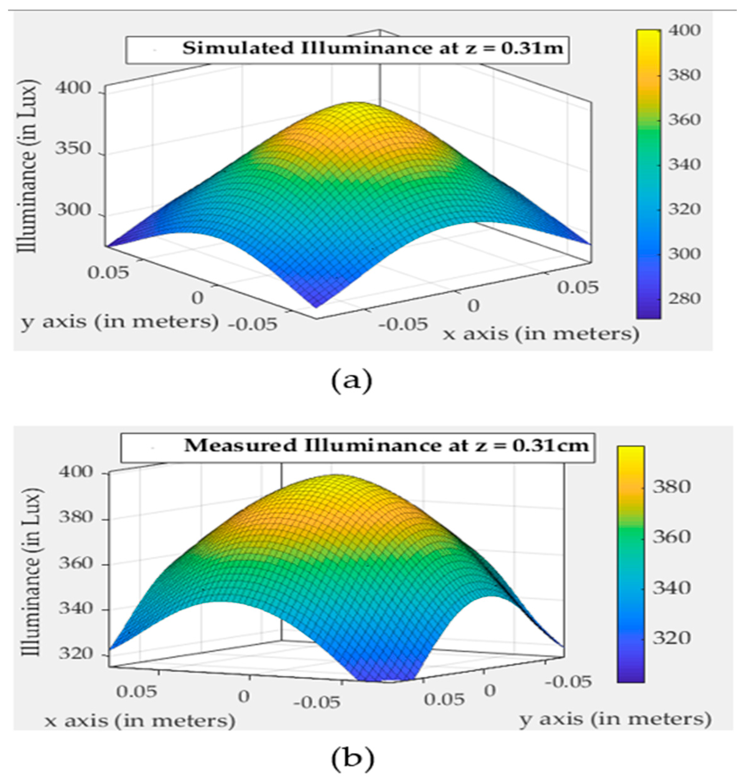
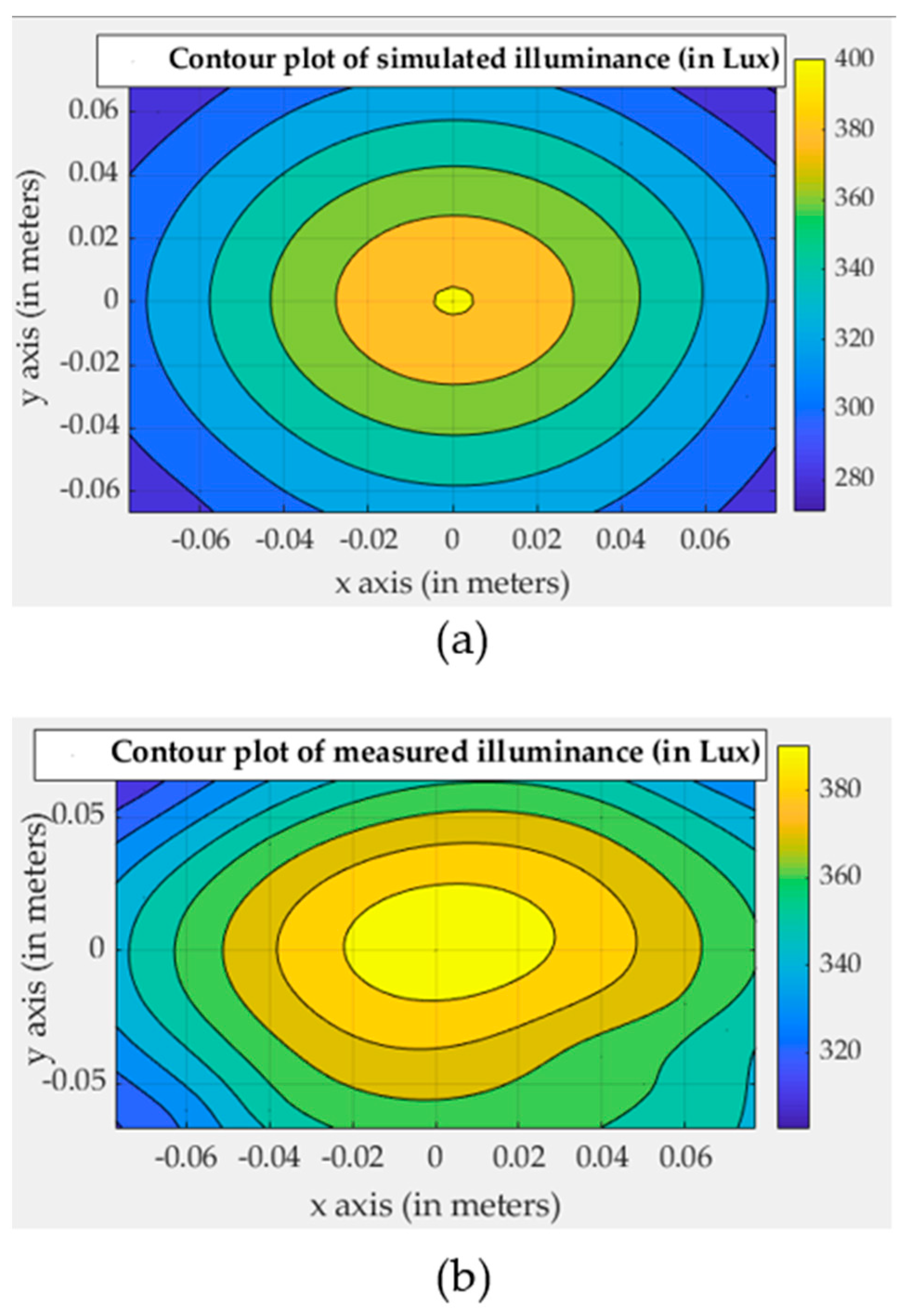
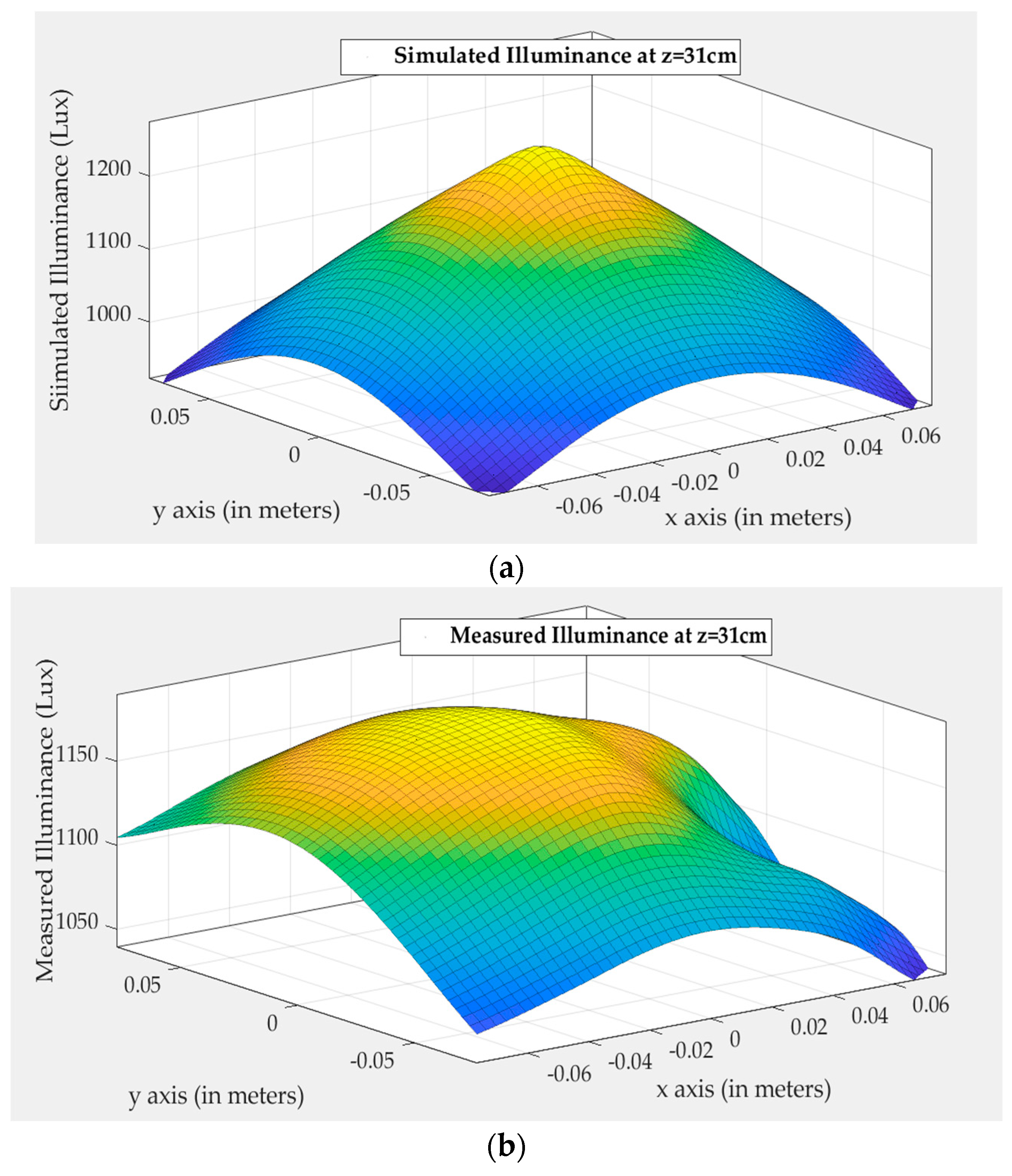
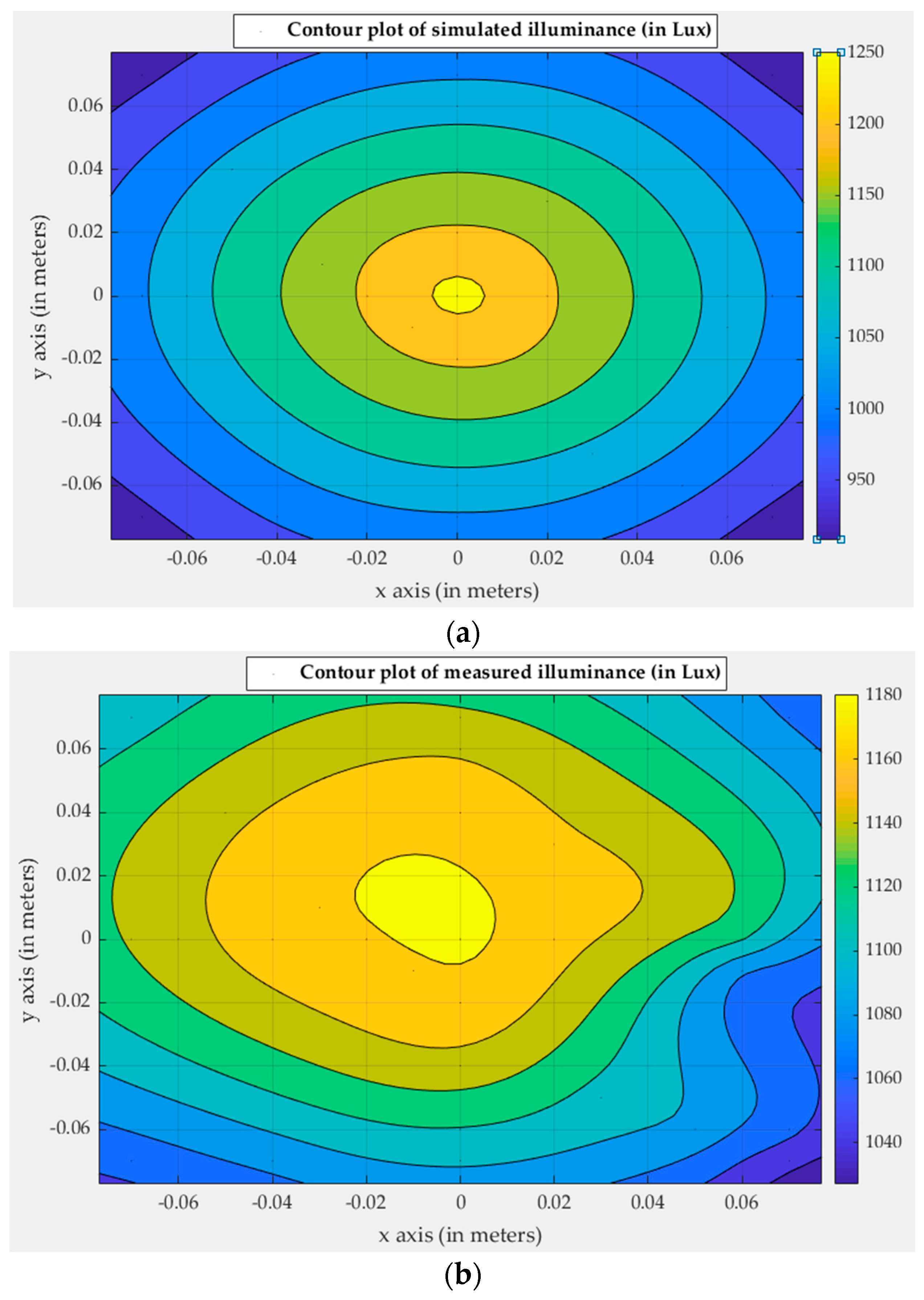
4.2. Simulations vs. Measurements

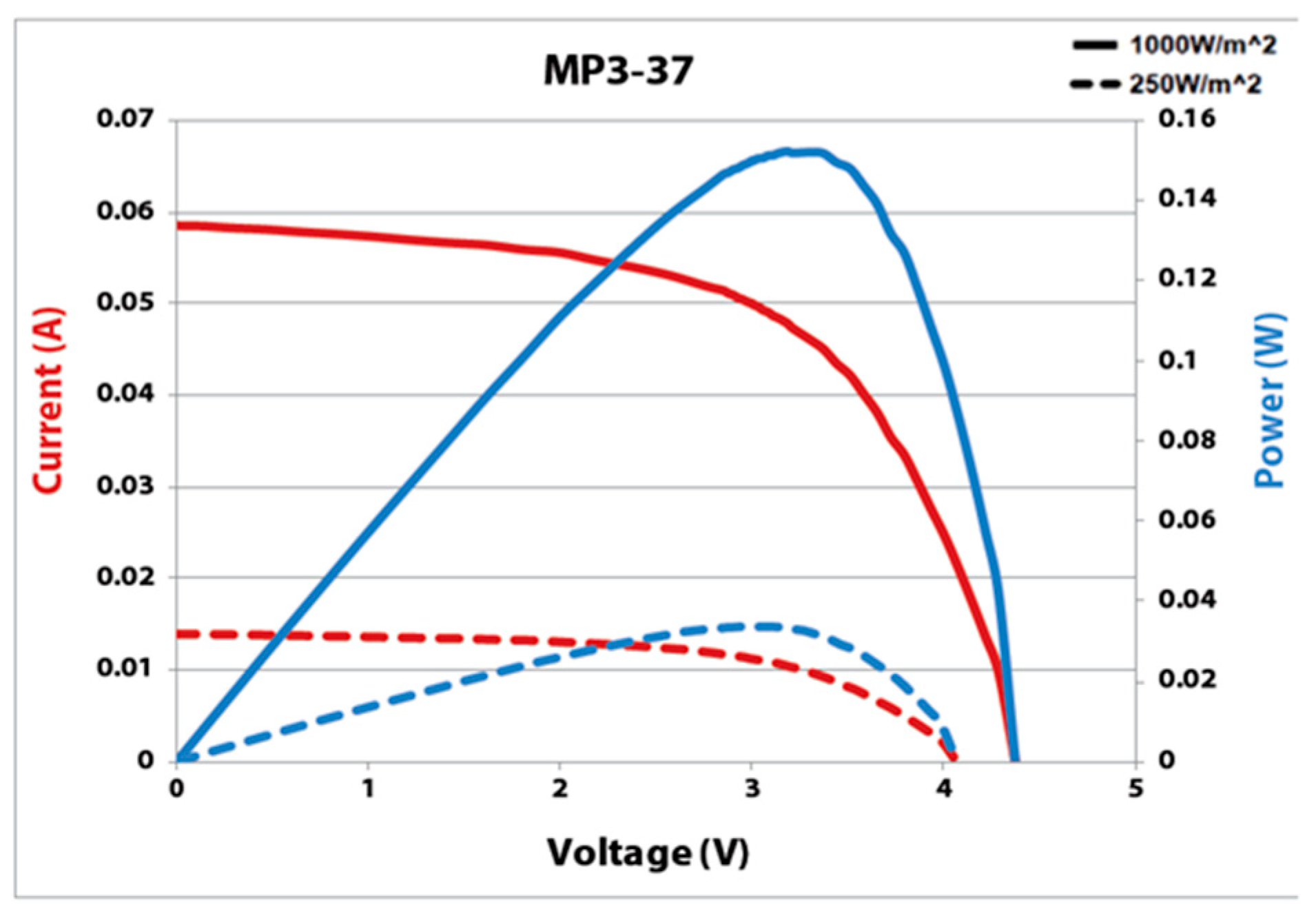
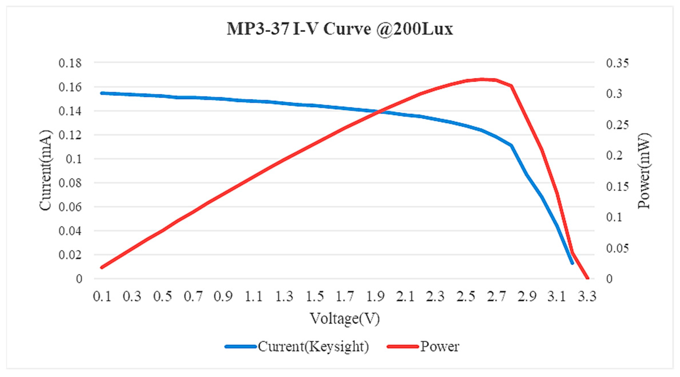
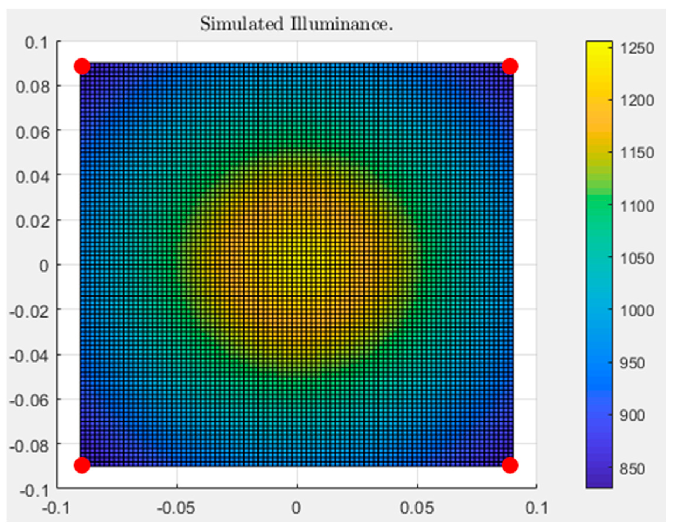
4.2.1. Single LED Measurements

In the first stage, an algorithm was developed with the capability to approximate and simulate all the quantities of interest. This algorithm takes as input the dimensions of the illuminated surface, the distance between the surface and the light source, and the full width at half maximum (FWHM) parameter and is capable of extracting the expected maximum and minimum values of irradiance and illuminance. Moreover, the algorithm can compute the non-uniformity of irradiance throughout the entire irradiated surface and determine the dimensions of the surface that can be illuminated for specific non-uniformity values. The latter is a fundamental criterion for the characterization and classification of light simulators. Additionally, it generates graphical representations of the irradiance and illuminance distributions for all the aforementioned cases.
The ensuing graphs depict the results obtained from a simulation performed considering the LED to be placed at the center of a surface with dimensions of 18 × 18 cm. The illuminated surface had dimensions of 14 × 14 cm, and a distance of 31 cm was maintained between the light source and the illuminated surface. All these variables are concentrated in Table 2.
In Figure 6 shows the simulated illuminance over the test plane. More specifically, the results obtained after comparing the simulation and the measurements are presented graphically in Figure 7. Figure 8 shows the contour plots for the same conditions.
Upon analysis of the graphs depicting the curves and contour plots of the measurements and simulations, it is evident that a significant level of convergence exists between the two. However, any observed deviations may be attributed to reflections caused by the light simulator.

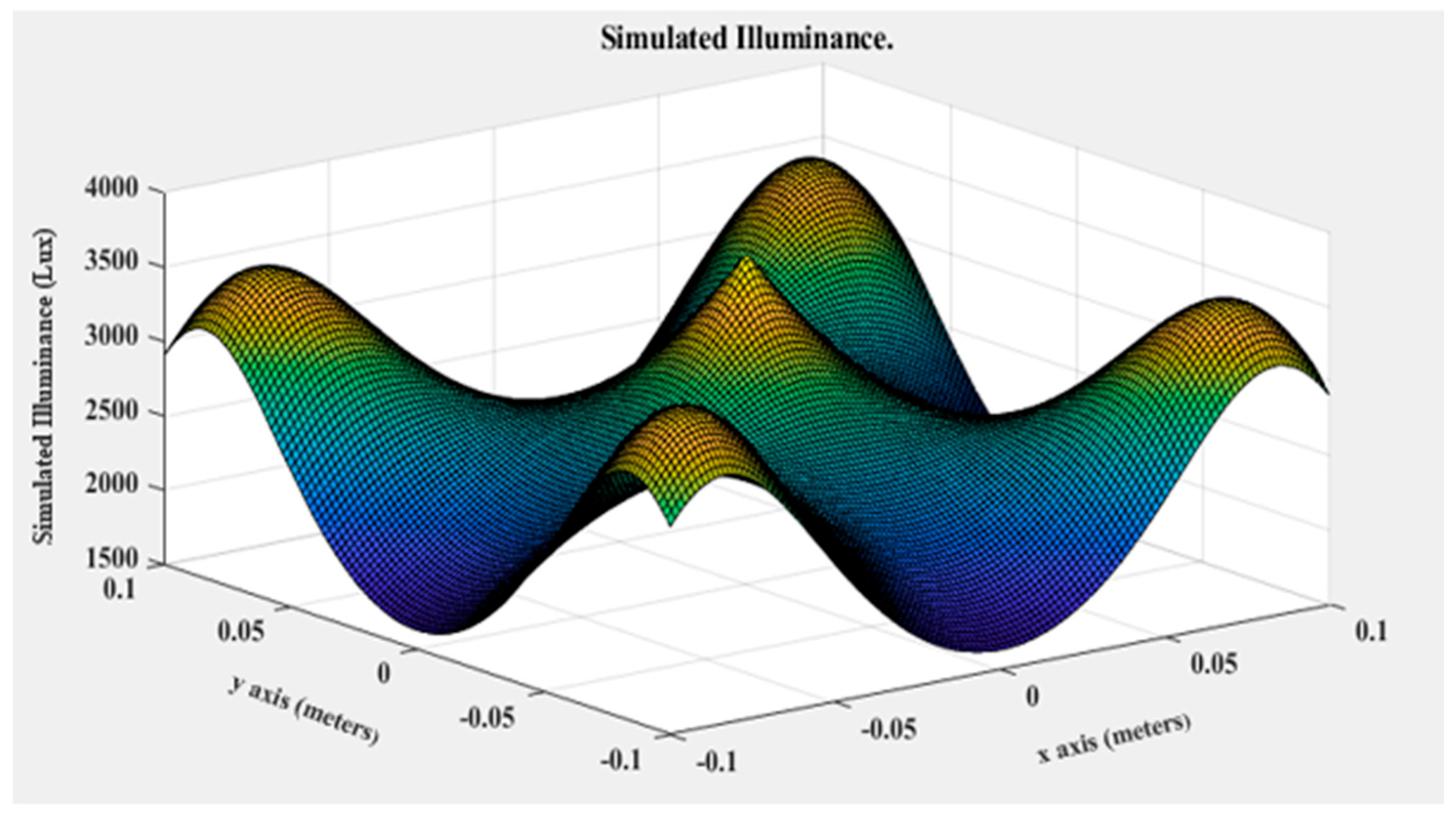
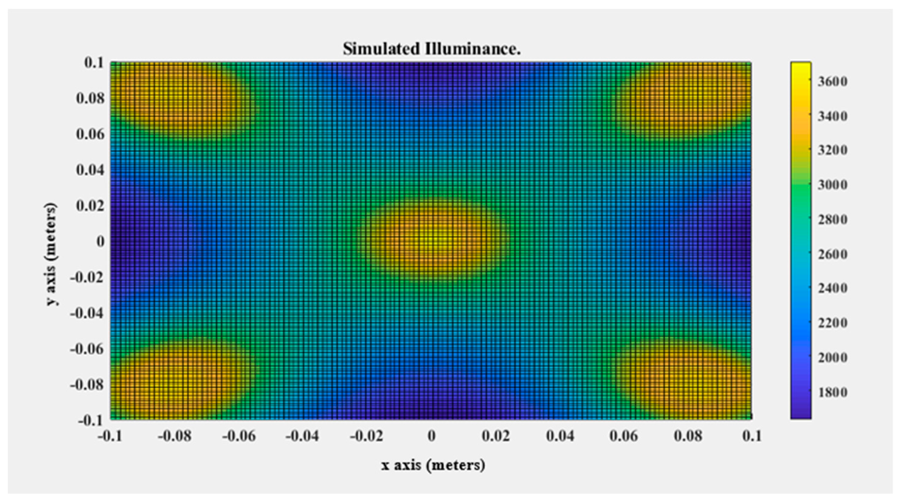
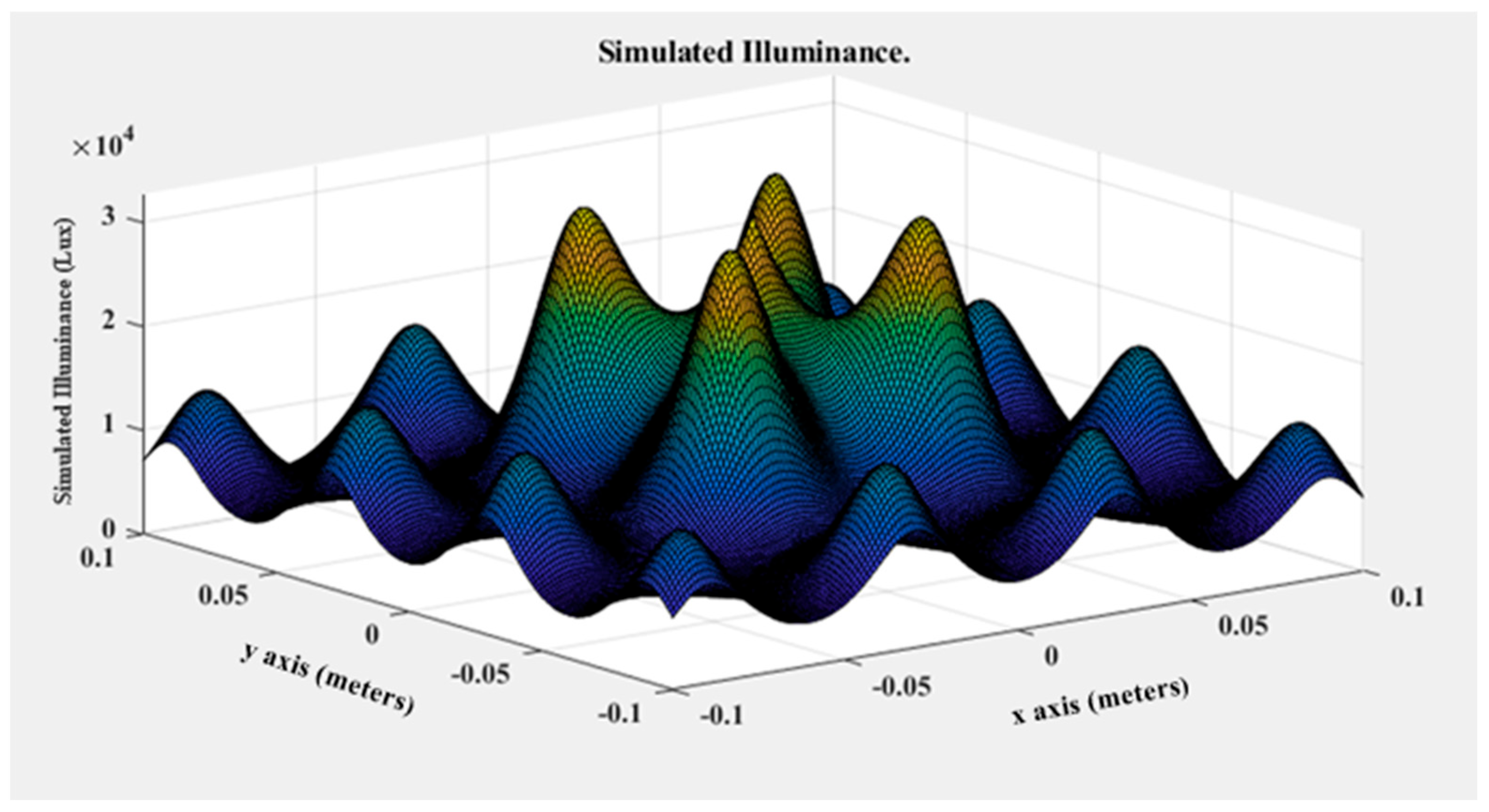
4.2.2. Multi-LED Measurements
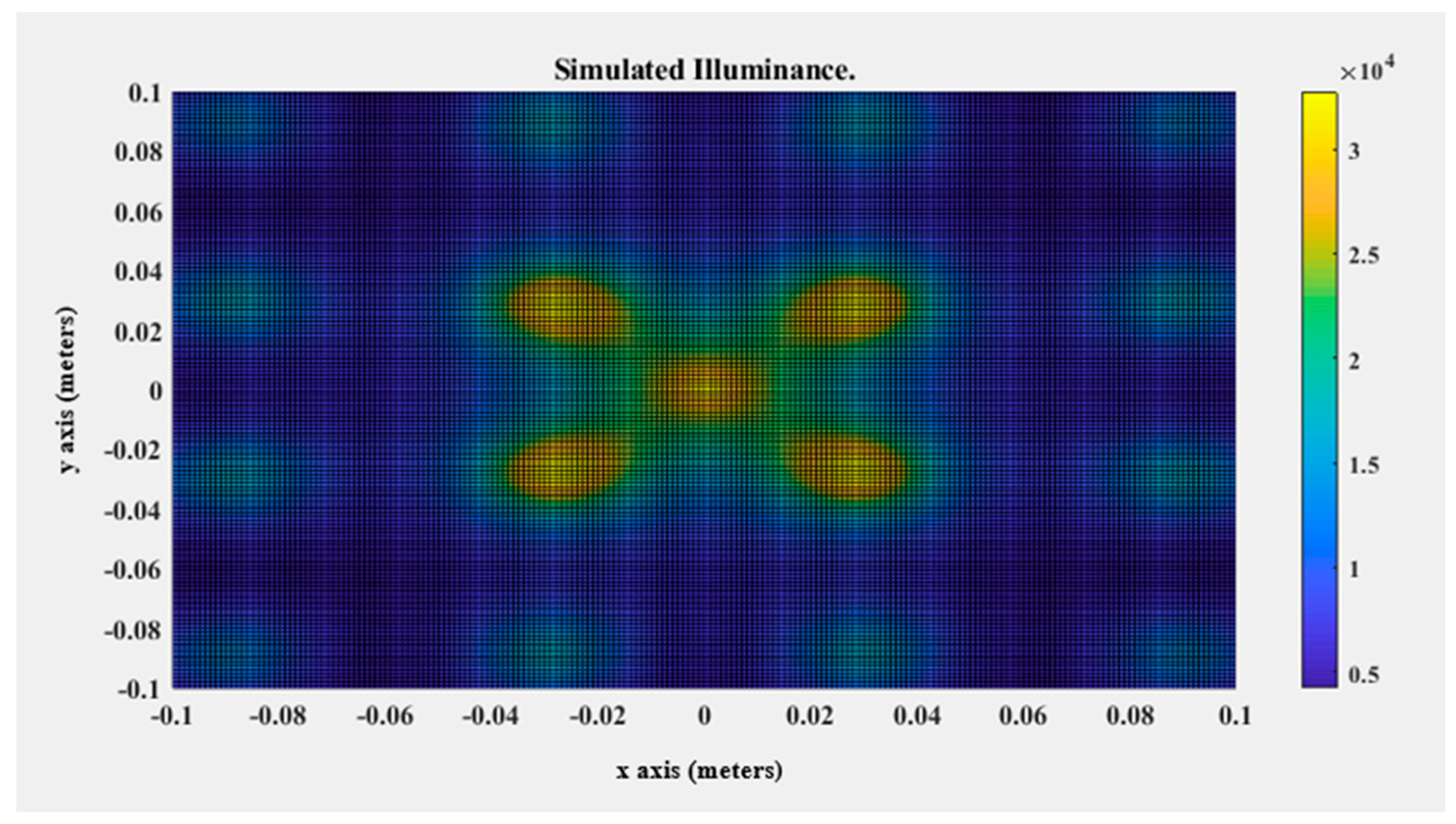
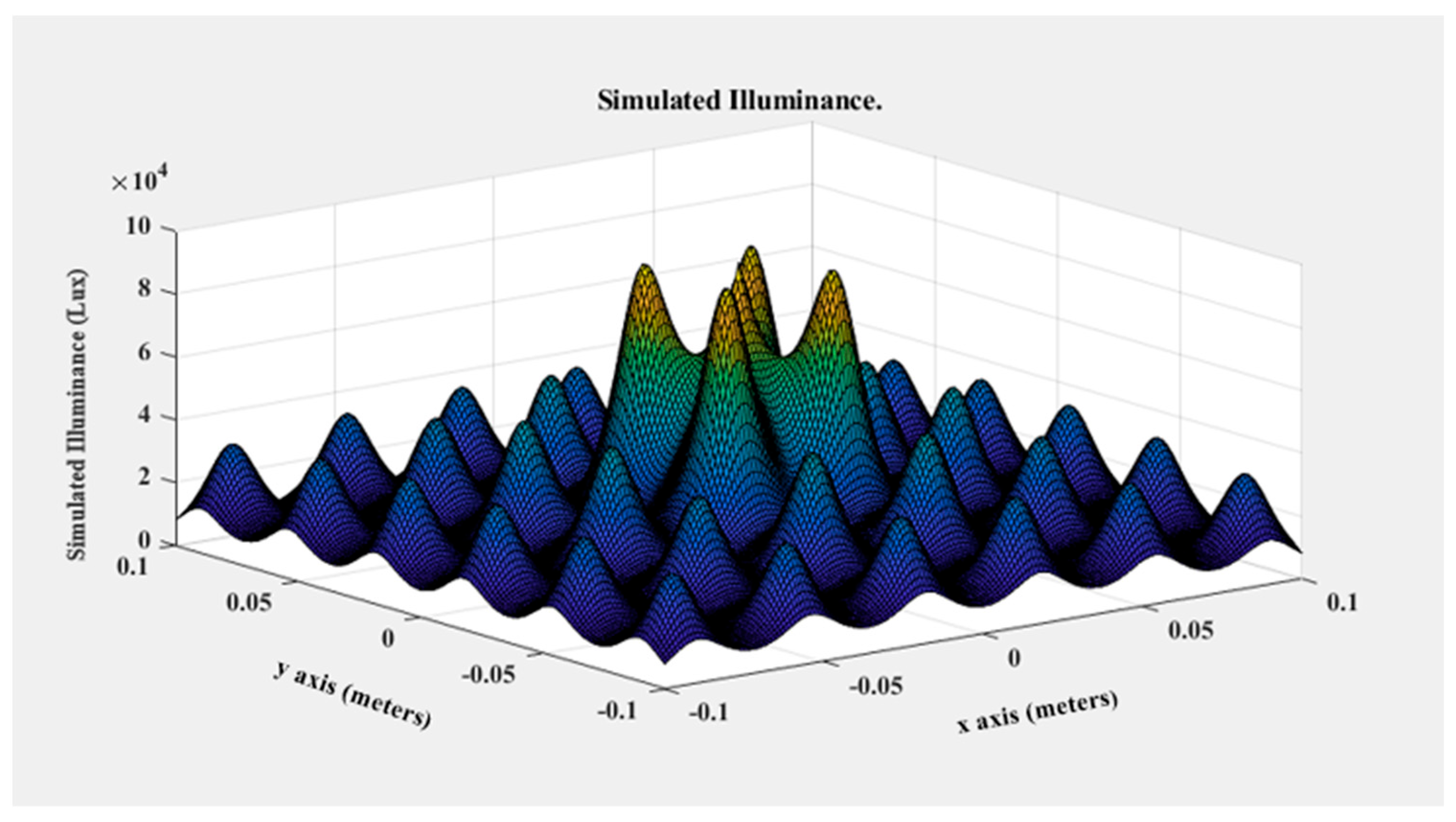
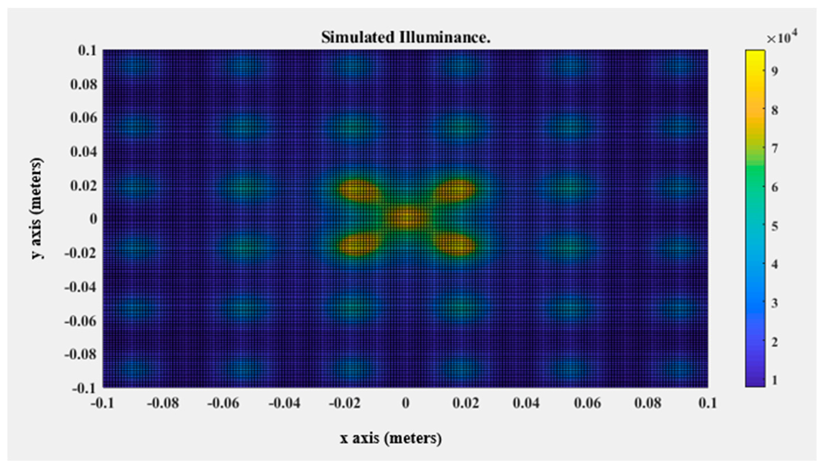
Square LED Topology

The decision to investigate the arrangement in which the LEDs are arranged squarely was made based on the results obtained from the algorithm already discussed. To determine the ideal (suitable) LED position, the algorithm was tested with the following assumptions. In Figure 9, the placement position of the light sources as well as the results of the lighting modeling and the LED array are shown.
The square LED array is 31 cm from the surface, which measures 18 × 18 cm. The red dots are used to indicate the location of the LEDs on the graph. Additionally, the LEDs were selected using a 2 × 2 LED square arrangement, wherein the distance between the LEDs is 18 cm.
To ensure the understanding of the conclusions drawn by comparing the simulations made with the resulting measurements, we present the illumination curves (Figure 10) along with the contour plots (Figure 11).
In comparison with the simulated non-uniformity, we observe a minor variation in Figure 10b. Reflections and other physical factors (such as the measurement instrument’s inaccuracy, the light sources’ temperature, etc.) might be blamed for this variance. Despite the deviations, we observe that the values of the anticipated illumination determined via the simulation test are remarkably near to the illumination that was ultimately measured. For instance, the difference between the predicted and measured values at (0, 0), the center of the testing plane, is less than 70 Lux.

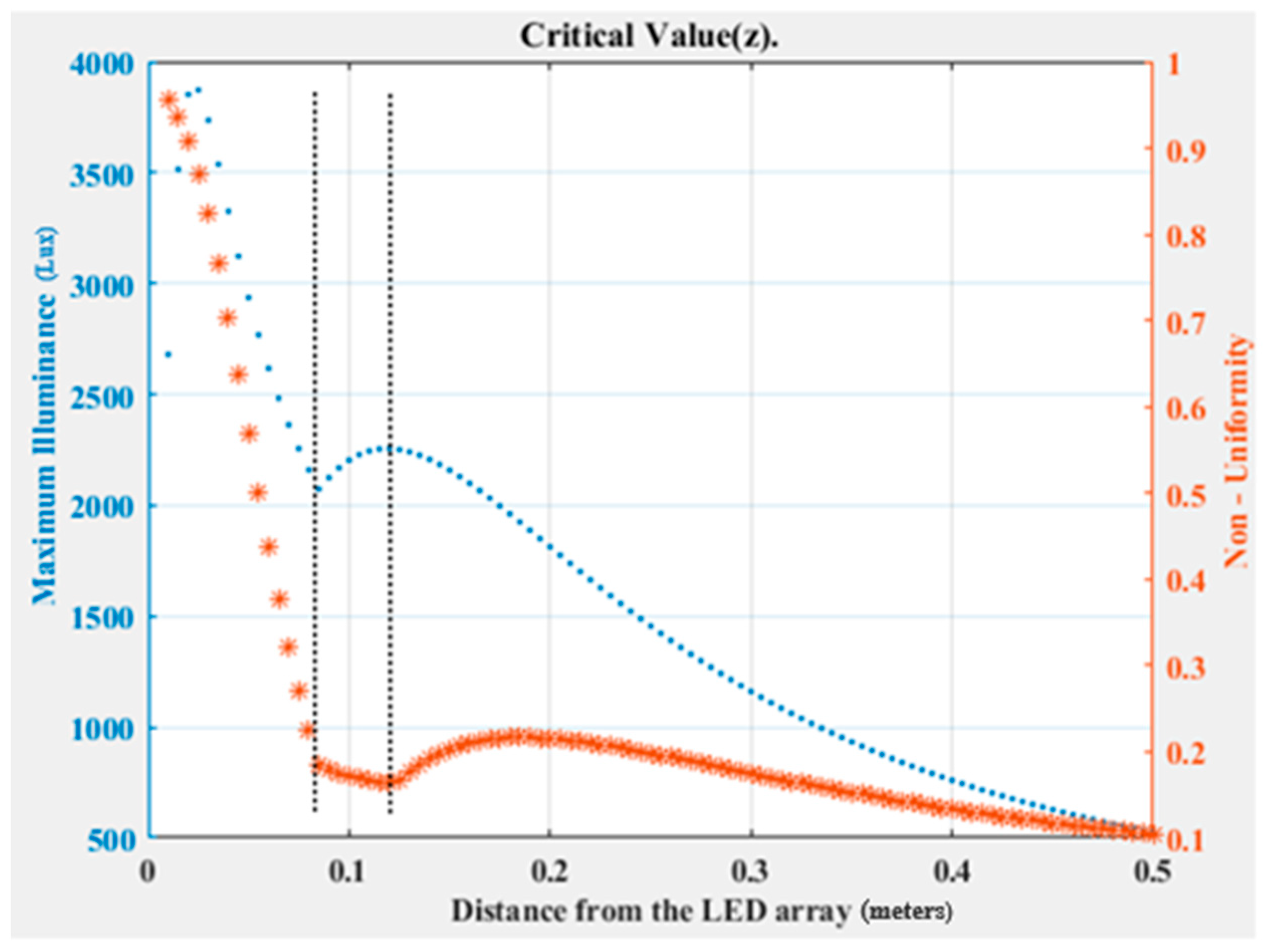
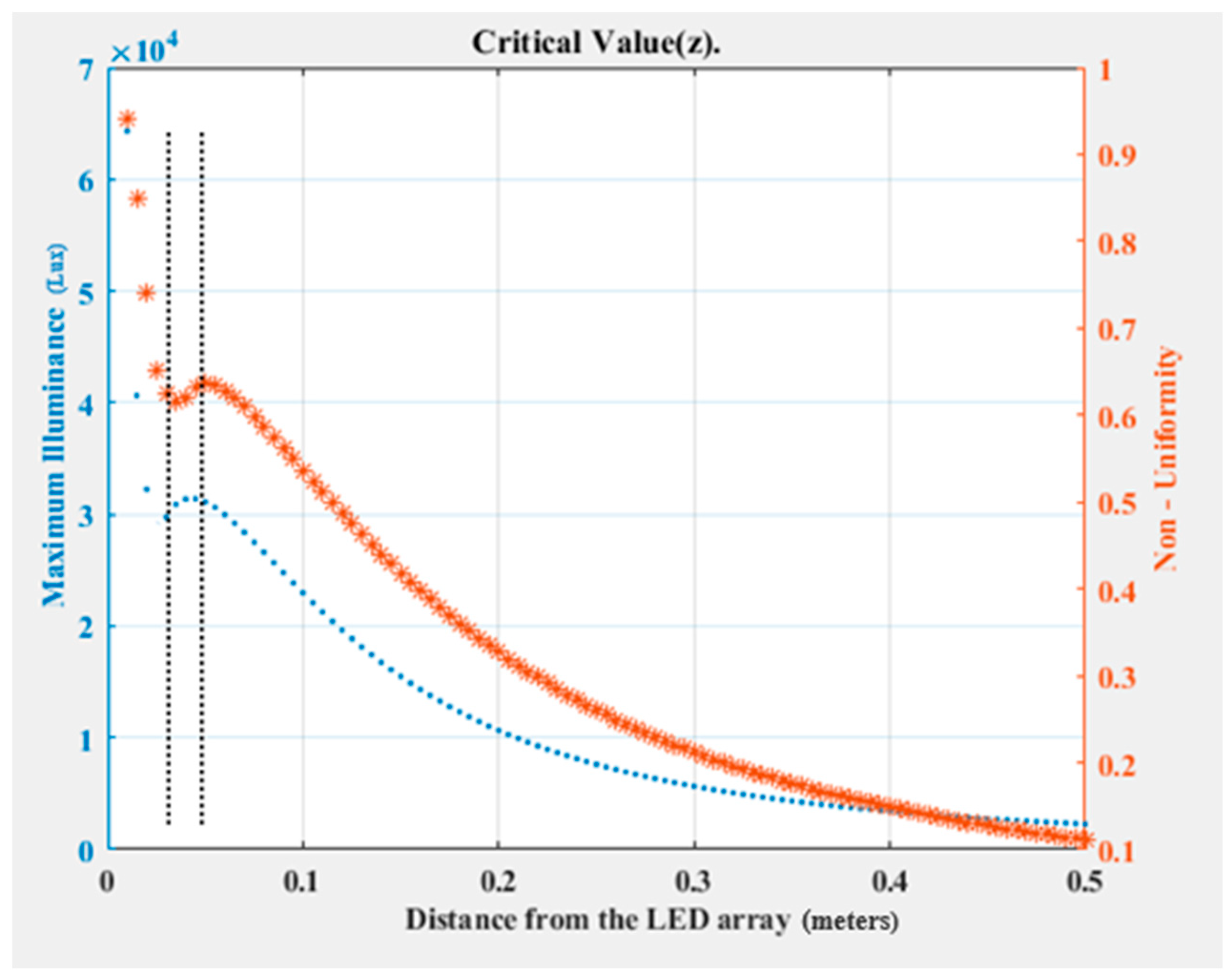
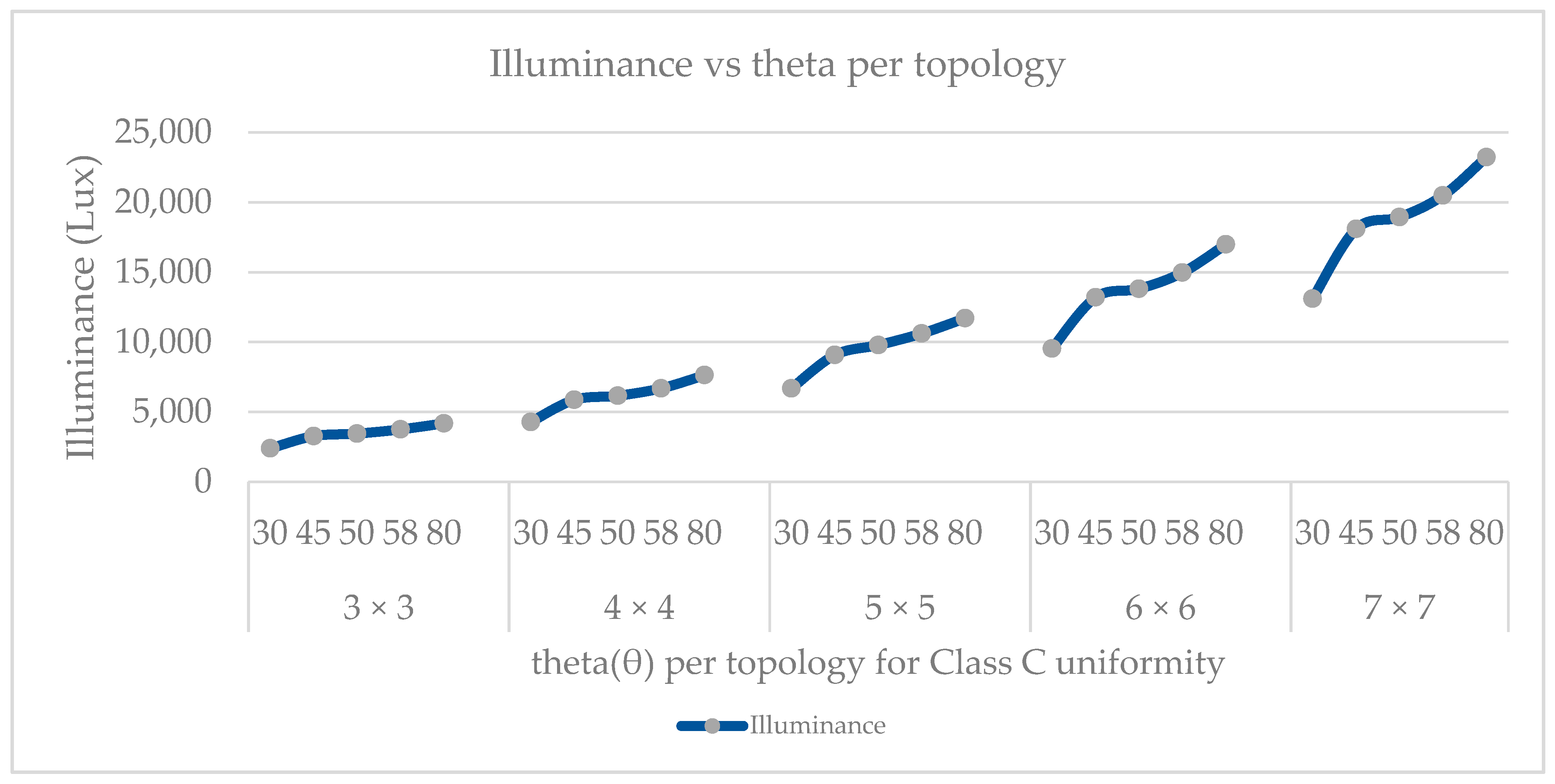
4.3. Multi-LED Light Simulator Design Guidelines’ Test

In order to verify the claims made regarding the design guidelines, we performed the test depicted in Table 3 [22]. As elucidated in Section 2.4, the examination of the critical value function (z) guided us to ascertain an interval denoted as [z1, z2], wherein the function exhibits monotonic changes.
First Case: Analysis of a Two × Two Light-Emitting Diode (LED) Array
During the examination, considering the available quantity of light sources, which was limited to four LEDs, the algorithm derives the optimal topology and the most suitable distance between them, complying with the restrictions imposed on the testing plane.
Subsequently, once the fundamental parameters have been established, the critical value function is evaluated. Through the analysis of this function, the turning point is determined which led to finding the interval [z1, z2] (shown by the black dashed lines) from which z0 was chosen (Figure 12).
Eventually, by substituting the turning point into the illuminance (or irradiance) distribution calculation algorithm, the graphical representation of the test plane under the calculated conditions is obtained (Figure 13 and Figure 14).
Second Case: Analysis of a Four × Four Light-Emitting Diode (LED) Array.
During the examination, the quantity of available light sources was limited to sixteen LEDs. The algorithm derives the optimal topology and the optimal inter-LED distance while adhering to the constraints imposed on the testing plane.
After setting the baseline parameters, the critical value function is evaluated, and subsequently, the turning point is obtained via analysis of the aforementioned function. This point led to finding the interval [z1, z2] (shown by the black dashed lines) from which z0 was chosen (Figure 15).
Subsequently, by substituting the turning point into the illuminance (or irradiance) distribution calculation algorithm, a graphical representation of the test plane under the calculated conditions is obtained (Figure 16 and Figure 17).
Third Case: Analysis of a Six × Six Light-Emitting Diode (LED) Array
In this investigation, a total of thirty-six LEDs were utilized as the available light sources. The algorithm successfully determines the optimal topology and inter-LED distance while considering the limitations imposed on the testing plane.
Once the baseline parameters have been established, the critical value function is evaluated. Through analysis of this function, the turning point is identified which led to finding the interval [z1, z2] (shown by the black dashed lines) from which z0 was chosen (Figure 18).
Subsequently, by substituting the turning point into the illuminance (or irradiance) distribution calculation algorithm, a graphical representation of the testing plane is generated based on the calculated conditions (Figure 19 and Figure 20).
After conducting an analysis of various LED array topologies, we came to several findings related to the optimization of illumination uniformity and maximum irradiance values. Through a series of rigorous tests and mathematical models, we identified the optimal non-uniformity that can be achieved while taking into account the maximum illuminance in specific intervals.
Our investigation demonstrated that a square LED array configuration provides the most favorable conditions for achieving optimal illumination uniformity and maximum irradiance values. The utilization of this configuration allowed us to evaluate different parameters, such as the number of LEDs required to achieve the desired illumination, the distance between the LEDs, and the angle at which light emanates from each LED. By taking these parameters into account, we were able to design LED arrays that produce light with the desired illuminance levels and uniformity ratios.
Based on the results of our analysis, we found that the target non-uniformity can be achieved by balancing the height and topology and associating the maximum irradiance values. The results are summarized in Table 4.
The next task was to identify the maximum illuminated surface for a given non-uniformity. The results of the experimentation are tabulated below, with the non-uniformity of a 12 × 12 cm area illuminated with a square 2 × 2 array as the baseline (Table 5). The results dictate a non-linear relationship between the area and the maximum illuminance.
Taking into consideration the experimental findings as a reference, our research sought to expand its scope by examining the performance of non-uniformity in square arrays with sources employing narrower illumination patterns. Specifically, via simulation we varied the viewing angle (theta) of the LEDs, obtaining the results presented in Figure 21. Our study focused on a 9 × 9 cm surface with a non-uniformity of less than 10%. Through experimentation, we determined that the appropriate distance for illuminating the surface fell within the range of [26.5 cm, 34.5 cm]. These first indications imply that narrow beam patterns do not improve the maximum illuminance. However, more research is required, and potentially different topologies may later alter this finding.

5. Conclusions and Future Work

In this work, we presented an analytical approach for modeling the light intensity distribution over a plane at a variable distance from multiple light sources. We utilized this approach to model a light simulator consisting of a limited number of LED sources. We specifically investigated the challenge of minimizing non-uniformity, leading to the stabilization of the irradiance distribution over a test area with specific dimensions. The above-mentioned findings were validated through experimentation conducted on a real light simulator setup.
We demonstrated that even with a small number of low-cost LED sources, high levels of irradiance can be achieved with bounded nonuniformities. The presented guidelines serve as a resource for designing tailored, low-cost light simulators that meet user-specific area/intensity/uniformity specifications. This work has the potential for application in various scientific and industrial domains including PV cell characterization, optics quality testing, education, DIY laboratory equipment, etc.
Future work should involve the incorporation of optics to examine light sources with varying viewing angles, including those with narrow and wide full width at half maximum (FWHM) angles, as well as investigating their potential synergistic effects. Building upon the conclusions derived from the present study, the inclusion of dimming LEDs in the center of the designated area is proposed as a promising improvement to achieve better uniformity smoothing.
Finally, a future study should involve the combination of LED sources with different spectrum responses, targeting the spectral emulation of different indoor light sources. This will improve the reliability of the estimation of PV cell performance in various indoor environments.

Author Contributions

Conceptualization, V.N., G.D. and I.M.; methodology, V.N., G.D. and I.M.; software, V.N., G.D. and I.M.; validation, V.N., G.D. and I.M.; formal analysis, V.N., G.D. and I.M.; investigation, V.N., G.D. and I.M.; resources, V.N., G.D. and I.M.; data curation, V.N., G.D. and I.M.; writing—original draft, V.N., G.D. and I.M.; writing—review & editing, V.N., G.D. and I.M.; visualization, V.N., G.D. and I.M.; supervision, G.D. All authors have read and agreed to the published version of the manuscript.

Funding

This research was co-financed by the European Regional Development Fund of the European Union and Greek national funds through the Operational Program Competitiveness, Entrepreneurship, and Innovation, under the call RESEARCH–CREATE–INNOVATE (project code: Τ2EDK-00350).

Data Availability Statement

The data are available on request.

Acknowledgments

The light simulator used for the measurements was constructed by postgraduate students Christos Koutsos and Leonidas Skaltsonis [24]. The authors would like thank Christos Koutsos for his assistance in the setup of the illumination head.

Conflicts of Interest

The authors declare no conflict of interest.

Abbreviation

AbbreviationDefinitionUnit
RESRenewable energy source-
IoTInternet of Things-
PV cellsPhotovoltaic cells-
LEDLight-emitting diode-
SRCStandardized reporting condition-
FWHMFull width at half maximum-
θPolar anglerad
φAzimuth anglerad
I(θ,φ)Radiant intensityW/sr
EeIrradianceW/m2
EvIlluminanceLux
mPosition-dependent constant value for LED emission region-
dDistancem
supSupremum
infInfimum
UUniformity
NUNon-uniformity

References

  1. Madeti, S.R.; Singh, S.N. Monitoring System for Photovoltaic Plants: A Review. Renew. Sustain. Energy Rev. 2017, 67, 1180–1207. [Google Scholar] [CrossRef]
  2. Rahman, M.M.; Selvaraj, J.; Rahim, N.A.; Hasanuzzaman, M. Global Modern Monitoring Systems for PV Based Power Generation: A Review. Renew. Sustain. Energy Rev. 2018, 82, 4142–4158. [Google Scholar] [CrossRef]
  3. Al-Fuqaha, A.; Guizani, M.; Mohammadi, M.; Aledhari, M.; Ayyash, M. Internet of Things: A Survey on Enabling Technologies, Protocols, and Applications. IEEE Commun. Surv. Tutor. 2015, 17, 2347–2376. [Google Scholar] [CrossRef]
  4. Zanella, A.; Bui, N.; Castellani, A.; Vangelista, L.; Zorzi, M. Internet of Things for Smart Cities. IEEE Internet Things J. 2014, 1, 22–32. [Google Scholar] [CrossRef]
  5. Xu, L.D.; He, W.; Li, S. Internet of Things in Industries: A Survey. IEEE Trans. Ind. Inform. 2014, 10, 2233–2243. [Google Scholar] [CrossRef]
  6. Tellawar, M.; Chamat, N. An Exclusive Review on IoT Based Solar Photovoltaic Remote Monitoring and Controlling Unit. Int. Res. J. Eng. Technol. (IRJET) 2019, 6, 1520–1525. [Google Scholar]
  7. Narendra, N.; Harshitha, P.; Layana Shree, N.; Sushmitha, M.; Harshavardana, D. SOLAR PANEL ANALYSIS USING IOT AND IMAGE PROCESSING. Int. Res. J. Eng. Technol. (IRJET) 2021, 8, 1452–1455. [Google Scholar]
  8. Best Research-Cell Efficiency Chart. Available online: https://www.nrel.gov/pv/cell-efficiency.html (accessed on 24 May 2023).
  9. Bouclé, J.; Ribeiro Dos Santos, D.; Julien-Vergonjanne, A. Doing More with Ambient Light: Harvesting Indoor Energy and Data Using Emerging Solar Cells. Solar 2023, 3, 161–183. [Google Scholar] [CrossRef]
  10. PowerFilm, S. Electronic Component Solar Panels, MP3-37. Available online: https://www.powerfilmsolar.com/products/electronic-component-solar-panels/classic-application-series/mp3-37 (accessed on 24 May 2023).
  11. IEC 60904-1:2006|IEC Webstore|Water Management, Smart City, Rural Electrification, Solar Power, Solar Panel, Photovoltaic, PV, LVDC. Available online: https://webstore.iec.ch/publication/3872 (accessed on 24 May 2023).
  12. Solar Simulator|Low Price, Class AAA, Small Area. Available online: https://www.ossila.com/en-eu/products/solar-simulator (accessed on 24 May 2023).
  13. López-Fraguas, E.; Sánchez-Pena, J.M.; Vergaz, R. A Low-Cost LED-Based Solar Simulator. IEEE Trans. Instrum. Meas. 2019, 68, 4913–4923. [Google Scholar] [CrossRef]
  14. Moria, H. Radiation Distribution Uniformization by Optimized Halogen Lamps Arrangement for a Solar Simulator. J. Sci. Eng. Res. 2016, 3, 29–34. [Google Scholar]
  15. Irwan, Y.M.; Leow, W.Z.; Irwanto, M.; Fareq, M.; Amelia, A.R.; Gomesh, N.; Safwati, I. Indoor Test Performance of PV Panel through Water Cooling Method. Energy Procedia 2015, 79, 604–611. [Google Scholar] [CrossRef]
  16. Elgendy, M.A.; Sundaram, V.M.; Surati, B.U. Design and Construction of a Low Cost Photovoltaic Generator for Laboratory Investigations. In Proceedings of the 2013 International Conference on Clean Electrical Power (ICCEP), Alghero, Italy, 11–13 June 2013; pp. 79–83. [Google Scholar]
  17. Landrock, C.; Omrane, B.; Aristizabal, J.; Kaminska, B.; Menon, C. An Improved Light Source Using Filtered Tungsten Lamps as an Affordable Solar Simulator for Testing of Photovoltaic Cells. In Proceedings of the 2011 IEEE 17th International Mixed-Signals, Sensors and Systems Test Workshop, Santa Barbara, CA, USA, 16–18 May 2011; pp. 153–158. [Google Scholar]
  18. Yandri, E. Uniformity Characteristic and Calibration of Simple Low Cost Compact Halogen Solar Simulator for Indoor Experiments. Int. J. Low-Carbon Technol. 2018, 13, 218–230. [Google Scholar] [CrossRef]
  19. Li, G.; Xuan, Q.; Pei, G.; Su, Y.; Ji, J. Effect of Non-Uniform Illumination and Temperature Distribution on Concentrating Solar Cell—A Review. Energy 2018, 144, 1119–1136. [Google Scholar] [CrossRef]
  20. Moreno, I. Configurations of LED Arrays for Uniform Illumination. In Proceedings of the 5th Iberoamerican Meeting on Optics and 8th Latin American Meeting on Optics, Lasers, and Their Applications; SPIE: Porlamar, Venezuela, 2004; Volume 5622, pp. 713–718. [Google Scholar]
  21. Naskari, V.; Doumenis, G.; Koutsos, C.; Masklavanos, I. Design and Implementation of an Indoors Light Simulator. In Proceedings of the 2022 7th South-East Europe Design Automation, Computer Engineering, Computer Networks and Social Media Conference (SEEDA-CECNSM), Ioannina, Greece, 23–25 September 2022; pp. 1–6. [Google Scholar]
  22. Naskari, V. Modeling of Artificial Light Pv Cell Evaluation System; University of Ioannina: Arta, Greece, 2022. [Google Scholar]
  23. Moreno, I.; Avendaño-Alejo, M.; Tzonchev, R.I. Designing Light-Emitting Diode Arrays for Uniform near-Field Irradiance. Appl. Opt. 2006, 45, 2265–2272. [Google Scholar] [CrossRef] [PubMed]
  24. Κουτσός, Χ.; Σκαλτσώνης, Λ. Σχεδίαση και ανάπτυξη συστήματος αξιολόγησης επιδόσεων Φ/Β στοιχείων; Bsc, University of Ioannina: Arta, Greece, 2021. [Google Scholar]
  25. Luminus SST-20-WxH High Power SST Product Datasheet 2021. Available online: https://download.luminus.com/datasheets/Luminus_SST-20-WxH_Datasheet.pdf (accessed on 23 May 2023).
  26. Nasiri, A.; Zabalawi, S.A.; Mandic, G. Indoor Power Harvesting Using Photovoltaic Cells for Low-Power Applications. IEEE Trans. Ind. Electron. 2009, 56, 4502–4509. [Google Scholar] [CrossRef]
  27. Shao, H.; Tsui, C.-Y.; Ki, W.-H. The Design of a Micro Power Management System for Applications Using Photovoltaic Cells With the Maximum Output Power Control. IEEE Trans. Very Large Scale Integr. VLSI Syst. 2009, 17, 1138–1142. [Google Scholar] [CrossRef]
  28. LedsMaster LED Lighting. What is Light Uniformity? How to Calculate Lux Level Lighting Uniformity. 2019. Available online: https://www.ledsmaster.com/what-is-light-uniformity-how-to-calculate-lux-level-lighting-uniformity.html (accessed on 23 May 2023).
  29. He, Y.; Xiong, L.; Meng, H.; Zhang, J.; Liu, D.; Zhang, J. Analysis of Non-Uniformity of Irradiance Measurement Uncertainties of a Pulsed Solar Simulator. In Proceedings of the Optical Metrology and Inspection for Industrial Applications II; SPIE: Beijing, China, 2012; Volume 8563, pp. 273–277. [Google Scholar]
Figure 1. MP3-37 I/V curve [10].
Information 14 00316 g001
Figure 2. MP3-37 I/V curve (measurements).
Information 14 00316 g002
Figure 3. Cartesian and spherical coordinate systems.
Information 14 00316 g003
Figure 4. Schematic of a square array.
Information 14 00316 g004
Figure 5. The light simulator used. (a) Experimental setup; (b) LED array’s arrangement.
Information 14 00316 g005
Figure 6. Simulated illuminance.
Information 14 00316 g006
Figure 7. Comparison of illumination curves. (a) Expected illumination curve; (b) measured illumination curve.
Information 14 00316 g007
Figure 8. Comparison of contour graphs. (a) Expected irradiance contour graph; (b) measured irradiance contour graph.
Information 14 00316 g008
Figure 9. Simulated illuminance distribution.
Information 14 00316 g009
Figure 10. Comparison of illumination curves for the 2 × 2 LED array. (a) Expected illumination curve; (b) measured illumination curve.
Information 14 00316 g010
Figure 11. Comparison of contour graphs for 2 × 2 LED array. (a) Expected illuminance contour graph; (b) measured illuminance contour graph.
Information 14 00316 g011
Figure 12. Two × two LED array’s illuminance and non-uniformity vs. LED array height.
Information 14 00316 g012
Figure 13. Illuminance distribution—critical value (0.081).
Information 14 00316 g013
Figure 14. Illuminance heatmap—critical value (0.081).
Information 14 00316 g014
Figure 15. Four × Four LED array’s critical value.
Information 14 00316 g015
Figure 16. Illuminance distribution—critical value (0.031).
Information 14 00316 g016
Figure 17. Illuminance heatmap—critical value (0.031).
Information 14 00316 g017
Figure 18. Six × six LED array’s critical value.
Information 14 00316 g018
Figure 19. Illuminance distribution—critical value (0.019).
Information 14 00316 g019
Figure 20. Illuminance heatmap—critical value (0.019).
Information 14 00316 g020
Figure 21. Illuminance vs. theta per topology.
Information 14 00316 g021
Table 1. Commercial solar simulators.
NameSpatial Non-Uniformity (Class)Target Size Square (Side cm)Working Distance (cm)Price (USD)Lamp Wattage (W)
Sciencetech SF-300-AClass AAA<5.5 × 5.510–136850300
Sciencetech PSS2Class AAA>50 × 507.590,000-
WaveLabs Sinus-70Class A+5.1 × 5.138-270
G2V Pico DIR-BASEClass AAA2.5 × 2.57-220
Oriel SOL-UV-6Class AAA15.2 × 15.215.24-1600
Table 2. System variables.
Dimensions of Illuminated Surface (m)Height (m)LED Array’s Dimensions (m)Radiometric Flux (mW)
φe442
x-axis[−0.07, 0.07]z-axisx-axis[−0.09, 0.09]Viewing Angle (degrees)
y-axis[−0.07, 0.07]0.31y-axis[−0.09, 0.09]2 ϑ/2120
Table 3. Square LED topological examination.
TopologyDistance between LEDs
(m)
Z0
(m)
2 × 20.180.078
4 × 40.060.031
6 × 60.0360.019
Table 4. Design guidelines results.
TopologyInterval of Distance from LED Array—Height (m) Interval of Non-UniformityInterval of
Max-Illuminance
(lux)
2 × 2[0.078, 0.121][0.162, 0.181][2080, 2270]
4 × 4[0.023, 0.048][0.62, 0.63][32,900, 30,800]
6 × 6[0.012, 0.041][0.71, 0.735][81,500, 83,000]
Table 5. Investigation of the results of design guidelines.
TopologyDistance from LED Array—Height (cm)Selected Centered Test Plane (cm)Non-Uniformity of the Selected Test Plane (%)Maximum Illuminance (lux)
2 × 212.112 × 1218.262270
3 × 397 × 717.5912,380
4 × 44.84 × 417.2930,800
5 × 54.553.3 × 3.317.2571,260
6 × 64.13 × 317.1283,000
Disclaimer/Publisher’s Note: The statements, opinions and data contained in all publications are solely those of the individual author(s) and contributor(s) and not of MDPI and/or the editor(s). MDPI and/or the editor(s) disclaim responsibility for any injury to people or property resulting from any ideas, methods, instructions or products referred to in the content.

