
Liver CT Image Recognition Method Based on Capsule Network

School of Computer & Information Engineering, Central South University of Forest & Technology, Changsha 410000, China
*
Author to whom correspondence should be addressed.
Information 2023, 14(3), 183; https://doi.org/10.3390/info14030183
Submission received: 19 January 2023
/
Revised: 13 February 2023
/
Accepted: 18 February 2023
/
Published: 15 March 2023
(This article belongs to the Special Issue Deep Learning for Human-Centric Computer Vision)
Abstract
:The automatic recognition of CT (Computed Tomography) images of liver cancer is important for the diagnosis and treatment of early liver cancer. However, there are problems such as single model structure and loss of pooling layer information when using a traditional convolutional neural network to recognize CT images of liver cancer. Therefore, this paper proposes an efficient method for liver CT image recognition based on the capsule network (CapsNet). Firstly, the liver CT images are preprocessed, and in the process of image denoising, the traditional non-local mean (NLM) denoising algorithm is optimized with a superpixel segmentation algorithm to better protect the information of image edges. After that, CapsNet was used for image recognition for liver CT images. The experimental results show that the average recognition rate of liver CT images reaches 92.9% when CapsNet is used, which is 5.3% higher than the traditional CNN model, indicating that CapsNet has better recognition accuracy for liver CT images.
1. Introduction
Liver cancer is currently the third leading cause of cancer death in men and the seventh leading cause of cancer death in women worldwide. According to statistics from related institutions, more than 700,000 people around the world die from liver cancer every year [1]. Early detection and effective treatment of liver cancer are important ways to increase the survival time of liver cancer patients. The CT examination has become one of the main methods for liver cancer detection because of the minor damage that it causes to the human body, its fast imaging, and its high accuracy. In the past, the processing of CT images relied on experienced doctors to give their judgment. However, through this method, the diagnosis will be affected by certain human uncertainties, which may cause misdiagnosis and delay the optimal treatment time for the patient. With the development of digital image processing technology [2,3] and pattern recognition technology [4] in recent years, more researchers have begun to research the application of computer recognition technology to CT images of liver cancer, achieving some results. Lee [5] used Gabor wavelet-generated texture features and SVM to distinguish normal tissues, cysts, hemangiomas, and carcinogenesis from CT images of liver cancer. Zhang [6] extracts the texture features of liver images from three aspects: first-order statistical features; gray-scale co-occurrence matrices; and gray-stroke matrices. Finally, the BP neural network designed by Zhang has a recognition rate of 91.08% for primary liver cancer. Liu [7] designed two kinds of classifiers for liver cancer identification through BP neural networks by extracting the texture and shape features of CT images of liver cancer, achieving a final recognition rate of 85%. Li [8] used the CNN model to identify liver tumors, ultimately also achieving relatively good recognition results. Meanwhile, Krishan [9] proposed two improved algorithms to enhance CT images before using SVM to classify liver CT images.
Based on the aforementioned references, past CT image recognition of liver cancer generally required researchers to specially design classifiers, which was time-consuming and provided different recognition accuracy depending on the researchers… The emergence of deep learning solves these aforementioned problems acceptably. Due to the characteristics that it possesses, such as local connectivity, weight sharing, and pooling operations, it allows for a significant reduction in the training network’s complexity and training parameters when compared with traditional liver cancer CT image identification methods [10,11]. However, the use of the CNN model to identify CT images of liver cancer results in the partial loss of useful feature information when employing the maximum pooling feature [12,13,14]. Furthermore, neurons are unable to characterize the spatial relationship between features. Thus, when the liver image is recognized using the CNN model, the overlapping of the images between the organs causes the deterioration of the learning feature’s effect, thereby affecting recognition accuracy. As a new framework for deep learning, CapsNet [15,16,17,18,19,20,21,22] encompasses many of the advantages of the CNN model. As CapsNet converts the scalar output of neurons into a vector output, the spatial relationship between liver tumor features can be well established by calculating the probability of the length and direction of the output vector. Therefore, this paper proposes a CT image recognition method based on the combination of an improved NLM and capsule networks. Firstly, the acquired liver images were pretreated. During the process of denoising the liver CT images, we improved strategic selection similar to the window of a traditional non-local mean denoising algorithm by introducing superpixel segmentation to protect the information on the edge of the image. Lastly, capsules were used to identify liver cancer in the CT images. The experiment’s results illustrate the effectiveness of this method.
2. Image Preprocessing
In the preliminary stage of liver CT image shooting and transmission, noise from the external environment will affect the image, so before recognition can be carried out on the image, it must be denoised to enhance the effect of recognition [23]. There are many traditional denoising methods, one of which is NLM. This is a denoising method based on the concept of image self-similarity [24,25,26,27,28,29,30,31,32,33,34,35,36]. Its main principle is that any one pixel is central to the whole of its similar neighborhood. The pixel value of the target in the image can then be measured against the weighted average of all the other pixels. Setting p(i) and q(i) as the target pixels before denoising and after denoising, respectively. With i as the current center’s pixel index, the relationship of pixel points before and after denoising can be expressed by Formula (1).
where I is the collection of the central pixel point i. ω(i,j) is a weight function used to measure the similarity between pixel points i and j. Its definition is shown in Formula (2).
represents the window with index i in a similar window. is the normalized factor. Meanwhile, H is the attenuation function of the weight function, its value is dependent on the noise intensity.
Since NLM can better preserve image details while denoising, we can use it to denoise liver CT images. The choice of a similar window size in the traditional NLM algorithm will affect the filtering effect. In the past, the choice of similar windows was often determined by experience, but this approach has great uncertainty. If the size of similar windows is too large, the denoising performance will be reduced and the computational complexity will be increased. If a similar window is too small, the color and structural features of the domain pixels are not well represented. To denoise the liver image effectively, we have improved the selection strategy of the similar window of the traditional NLM denoising method by introducing superpixel segmentation.
3. NLM Liver CT Image Denoising Method Based on SLIC Algorithm
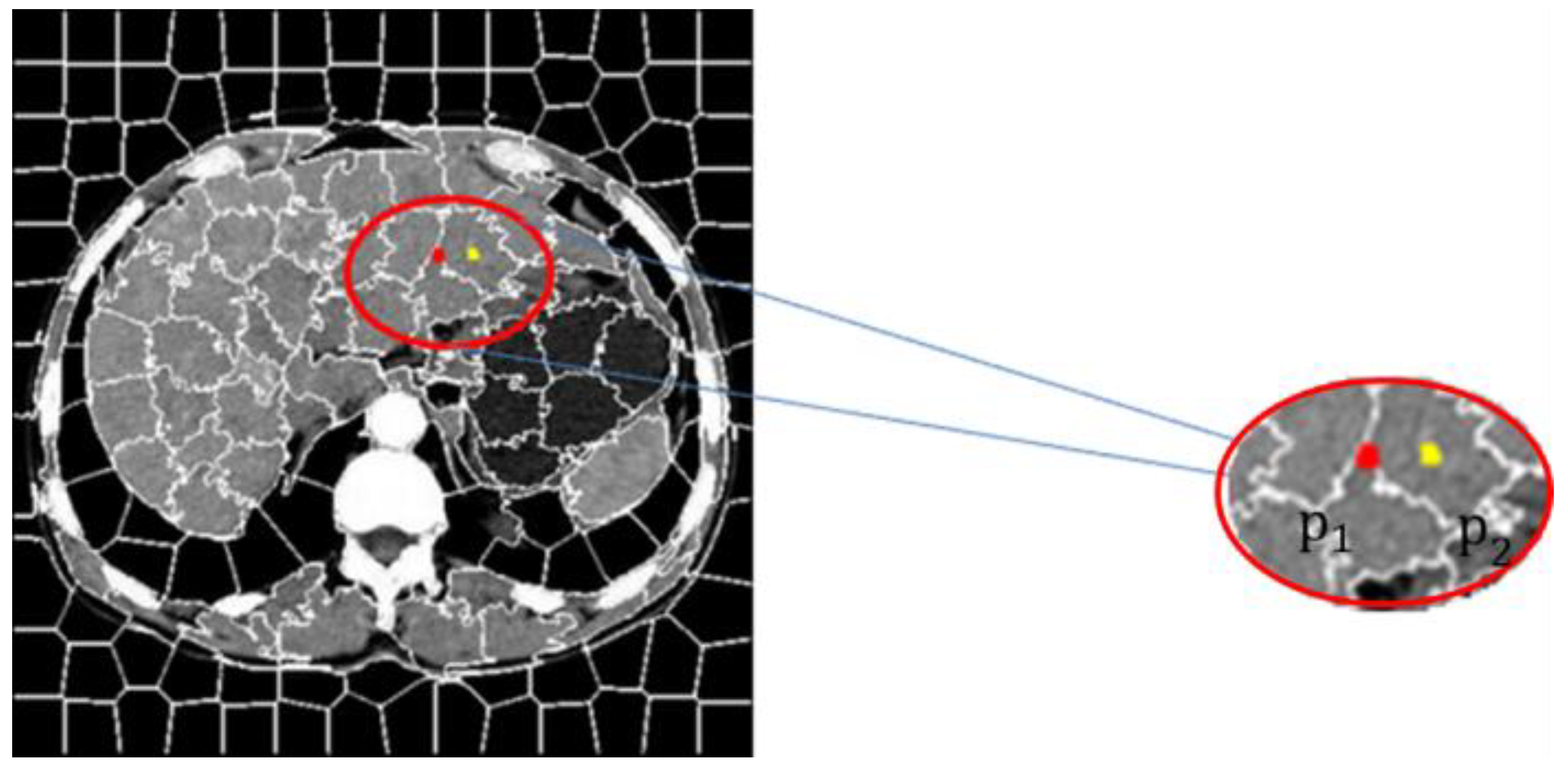
The SLIC segmentation algorithm was used to segment the liver CT image that contained noise with superpixel segmentation and a few image blocks that contained internal similarities from the original image was created, obtaining a textured outline of the image containing noise. The central target pixel to be restored, p(i) is selected to judge whether the center pixel point is located inside the superpixel segmentation block or on the outer line of it according to the texture contour map. As shown in Figure 1, p1 and p2 represent the central pixel points located at the edge of the superpixel and the inner pixel respectively.
Different similar window selection strategies and sizes are adopted according to the structural characteristics of the central pixel’s position. Finally, the calculation formula of Formula (3) is used to calculate the similarity between each similar window and the central pixel block. Formula (2) calculates the weight of each similar block, and Formula (1) averages the similar Windows to obtain the pixel value q(i) after denoising.
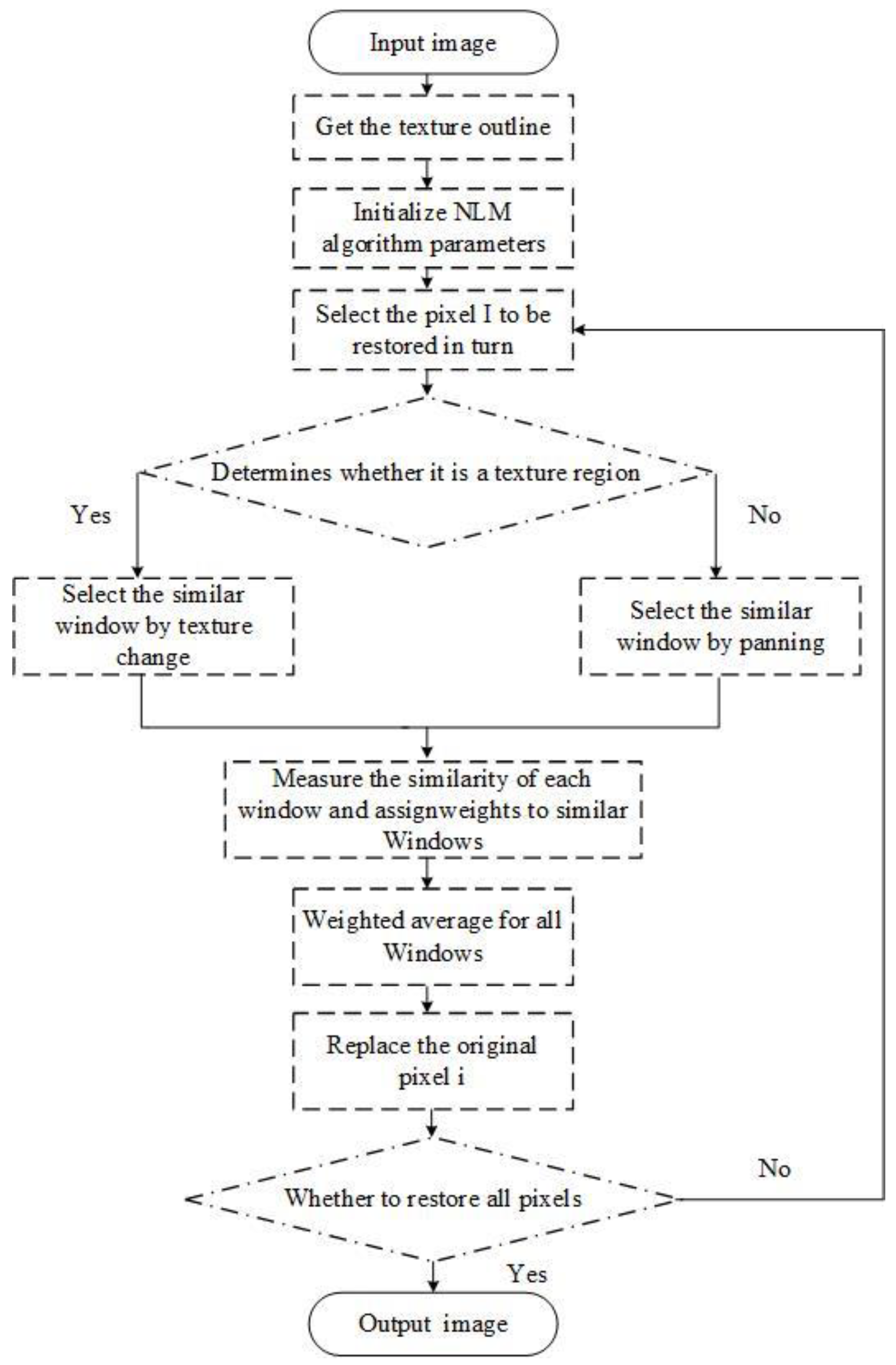
is the gaussian weighted Euclidean distance representing p(i) and q(i). a is the standard deviation of the gaussian kernel, a > 0. The flow chart of the entire algorithm is shown in Figure 2.
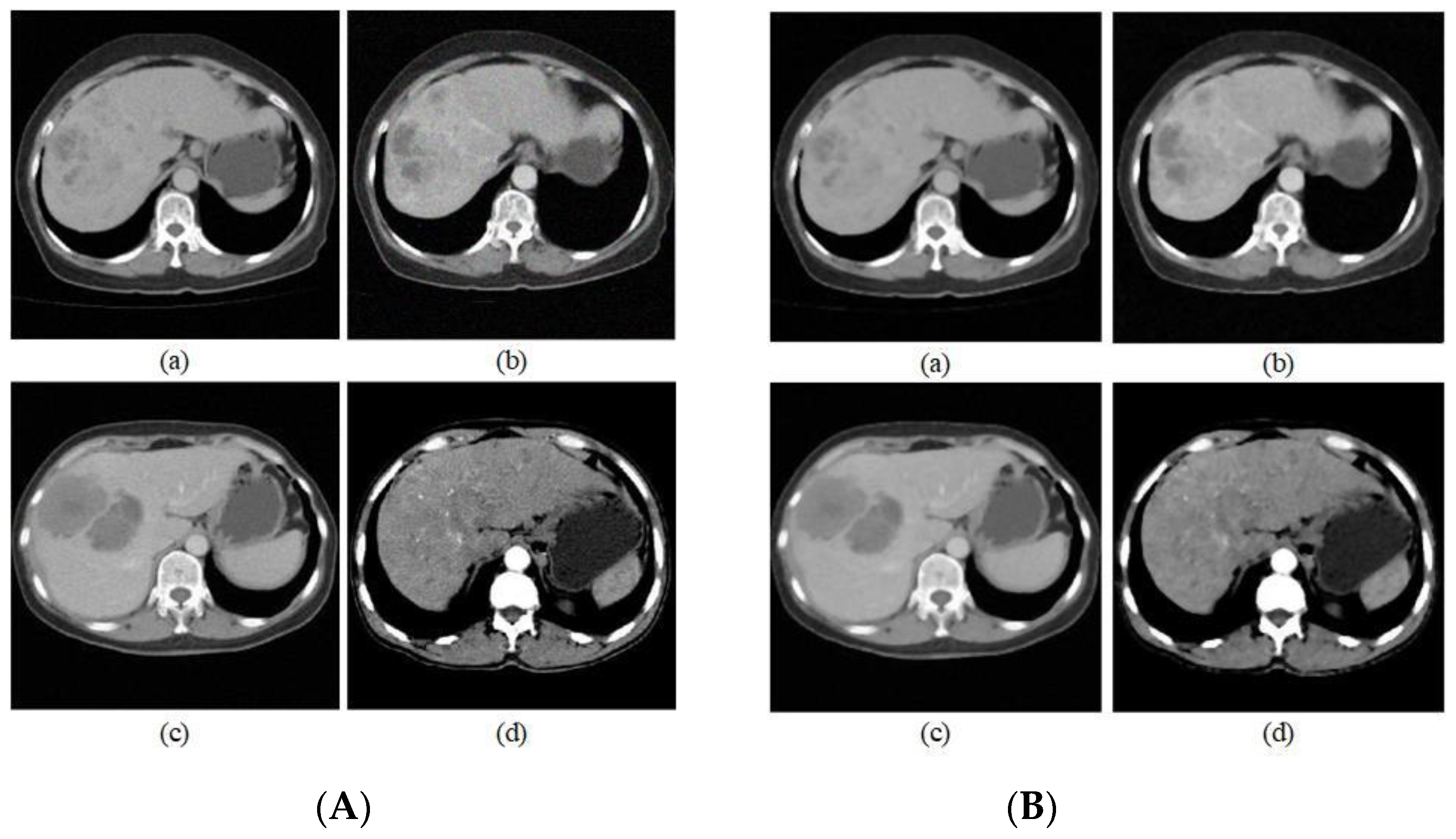
In the selection of the denoising parameters, we considered that a too large a window will result in too long a running time, thus we decided to use a 13 × 13-pixel size in consideration of time efficiency and set the smoothing parameter to 10. To more accurately measure similarity, when the central pixel was within a flat area, we selected a similar window of 7 × 7 and when the central pixel was on a contoured, outer line, we selected a similar window of 5 × 5. Figure 3 shows some CT images of the liver before and after denoising, respectively.
By comparing the CT images before and after denoising, the information at the edges of the images is well preserved compared with that before denoising, but the specific noise reduction effect cannot be observed by the human eye because the image size is small and the noise reduction effect exists at the pixel level. We verify the effectiveness of noise reduction by image noise reduction index. In addition, since the obtained liver CT images were of different sizes, they were all converted to 32 × 32 size after denoising for the convenience of subsequent operations.
PSNR (Peak Signal-to-Noise Ratio), is used to measure the difference between two images.
where MSE is the mean square error of the two images; MaxValue is the maximum value that can be obtained from the image pixels. And SSIM (Structural Similarity) assumes that the human eye will extract structured information from images, which is more consistent with human eye visual perception than the traditional approach.
where l(x,y) denotes the luminance share, c(x,y) denotes the contrast share, and s(x,y) denotes the structure share.
As can be seen from Table 1, the performance of this noise reduction algorithm is good, thanks to the combination of a realistic noise model and a realistic image. The PSNR/SSIM of this paper’s noise reduction algorithm is excellent for both PSNR and SSIM, and it performs well in terms of maintaining and balancing noise.
4. Liver Cancer Image Recognition
After the pretreatment of the liver cancer image is completed, it needs to be classified and identified. At present, existing image classification methods include recognition methods based on support vector machines and convolutional neural networks. This paper principally introduces the identification method based on capsule networks.
4.1. CapsNet
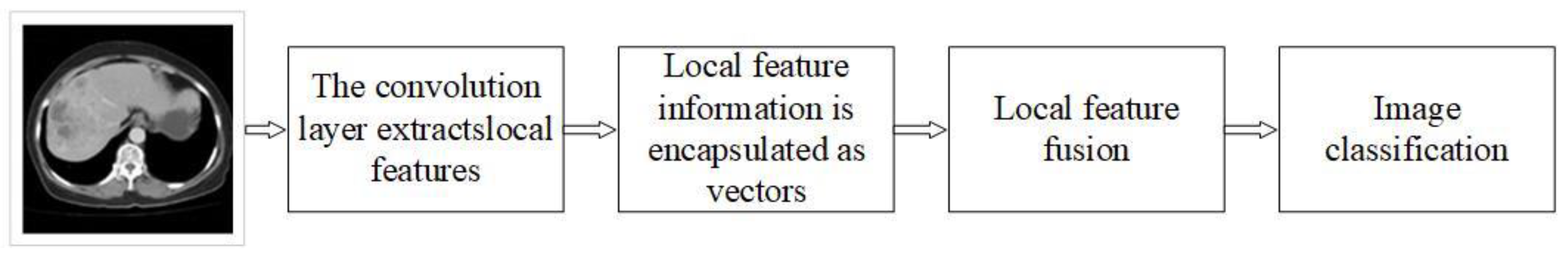
CapsNet [13] is a new deep-learning network framework proposed by Hinton. Similar to the traditional CNN model, CapsNet also extracts local features of liver images through convolutional layers. The difference is that CapsNet adds the Primary Caps layer after the convolutional layer, in which each local feature is converted to a vector containing spatial information and then imported into the next layer of capsules. Finally, the classification and reconstruction of the liver cancer images were achieved by fully connecting three layers. The entire identification process is shown in Figure 4.
In the selection of the activation function, unlike the activation functions ReLU and sigmoid in the convolutional neural network, the capsule network introduces a new nonlinear activation function squashing function to process the received vector to characterize the probability that the current entity exists in the current input. It not only scales the total input vector to a range of (0, 1), but also makes the direction of the input vector Sj and the output vector Vj consistent. The formula is as follows:
Vj represents the total output vector of j capsules, and Sj represents the total input vector of j capsules. The total output length of the squashing function represents the probability that the capsule will detect the specified feature.
On a hierarchical structure, the CapsNet covers the detected area by creating a higher-level capsule node. The active low-level capsule obtains the output vector by changing the scalar weight, before multiplying the weight and then sending the product to the high-level capsule; the high-level capsule then uses the received product as the input vector. The propagation formula of low-level capsules and high-rise capsules is shown in Equations (7) and (8).
Cij represents the weight between each lower layer capsule and its corresponding higher layer capsule, as determined by dynamic routing iterative selection, this weight is a non-negative scalar. For each lower layer capsule i, all weights Cij are determined by the softmax function in the dynamic routing algorithm employed. Its formula is as follows:
bij is a given temporary variable.
In terms of propagation mode, the dynamic routing algorithm between capsules adopts a forward propagation algorithm. The specific process is as follows:
Step 1: Determine the parameters of the algorithm and iteration times, r. To avoid excessive fitting in practical applications, an appropriate r value needs to be selected, the number of iterations selected in this paper is 3.
Step 2: At the beginning of training, a temporary variable Cij is first defined and initialized to 0. In the iterative process of the algorithm, bij will be updated continuously. After iterative acceptance, the value of bij is saved to Cij to update the routing coefficient between the lower capsule layer and the higher capsule layer.
Step 3: Iterate through the number of iterations of dynamic routing. In this process, the temporary variable bij, is first put into the softmax function to calculate the initial value of all low-level Cij capsules. Since bij is initialized to zero in the initialization process, all routing coefficients of Cij are equal when the weight is updated for the first time. In this process, all weights are guaranteed to be greater than or equal to 0, and the sum of all the weights of Cij is 1. Next, the output vector of all lower-layer capsules is determined with Sj. Next, the set output vector direction will remain unchanged, and the output vector’s modulus is scaled to within 1 neighborhood, this scaling process is determined by nonlinear function squashing. The resulting vector, Vj is the output of all high-level capsules. Finally, the essence of the dynamic routing algorithm between capsules is used to update the weights, primarily by obtaining the scalar product from the output, Vj of the high-level capsule, and the input, of the lower-layer capsule, before summing up the old weights to obtain new weights, the process of weight adjustment is to repeat the iteration r times. When the iteration is over, the low-level capsule determines its target high-level capsule and passes the output to the corresponding high-level capsule. By performing the above algorithm to train the capsule network, the scalar product of the vector is continuously used to update the routing coefficient, forward conduction can then be advanced to the higher layer network.
Similarly, to the convolutional neural network, the capsule network also needs to perform loss assessment to better improve the reconstruction speed and accuracy of the liver image. The loss function in the capsule network is similar to that of the SVM. When the input vector is classified and predicted using the length of the output vector in the digital capsule, the effect of the classifier will be better concurrently with a smaller loss value. Conversely, the classification effect is worse. The loss function used in the digital capsule layer is shown in Formula (10):
Lc represents the loss value of a single capsule, and λ is generally 0.5. Where Tc = 1 if a digit of class k is present 3 and m+ = 0.9 and m− = 0.1. The λ down-weighting of the loss for absent digit classes stops the initial learning from shrinking the lengths of the activity vectors of all the digit capsules. So, we set λ = 0.5. The total loss should be calculated by adding up the loss values of all individual capsules.
4.2. Network Structure
The capsule network structure used in this paper is based on the original capsule network proposed by Hinton, which can be divided into two parts: encoder and decoder. The encoder is primarily composed of convolution layers, a main capsule layer, and a digital capsule layer. The decoder consists of three fully connected layers. The structure is shown in Figure 5.
The first layer is the input layer, in which the CT image size of the liver is converted to 32 × 32 and binary data is input into the convolution layer. The second layer is the conventional convolution layer, this layer has 8 feature planes and 256 convolution verification images for feature extraction. The third layer is the main capsule layer, and the input of the main capsule layer is the convolution layer’s output after excitation function processing has been carried out. 32 capsules are used in this layer, each containing 8 parallel convolution units, sharing the weight, wij. The main capsule layer aggregates the features of the convolutional layer and determines the relative positional relationship of the individual features. During the process of selecting a convolution kernel, what must be considered is that if the convolution kernel is too small then the noise and the features will be enhanced together, and if the convolution kernel is too large, the quantity requiring calculation will be too great. To obtain a better recognition effect, during the experiment, we set the convolution kernel size of the conventional convolution layer and the main capsule layer as 8 × 8, 9 × 9, and 10 × 10 respectively before conducting a comparative experiment to explore the influence of convolution kernel size on the effect of liver image recognition. The fourth layer is a digital capsule layer. There are 2 capsules on this layer, each of which is a 16-dimensional vector. A dynamic routing algorithm is required between the primary capsule layer and the digital capsule layer to obtain a relationship between all of the capsules in the primary capsule layer and the capsules in the digital capsule layer that represent cancerous conditions in the liver. Through this method, all local features can be made to aid in characterizing the capsules in the digital capsule layer. In addition, for the output of the digital capsule layer, a function of introducing the loss function of Equation (8) is required to perform a loss assessment on the accuracy of the dynamic routing algorithm employed by the digital capsule layer. When the loss value is too large, the weight and routing parameters need to be adjusted, and then trained again to produce a better model.
5. Experiment
5.1. Experiment Preparation
The computer used in this article is a laptop with an Intel i5-CPU, 16GB of RAM, and a gtx1060-gpu. The software used is the Windows operating system with TensorFlow installed, which is used as a framework for deep learning. The data set used contained 1500 CT images of the liver pretreated by the improved algorithm above, with 750 images containing liver cancer, and 705 images containing a healthy liver. These liver datasets were collected from the Internet, most of them from LiTS—Liver Tumor Segmentation Challenge, https://competitions.codalab.org/competitions/17094 (accessed on 4 August 2017), and processed to obtain the final dataset for this paper.
5.2. Analysis of Experimental Results
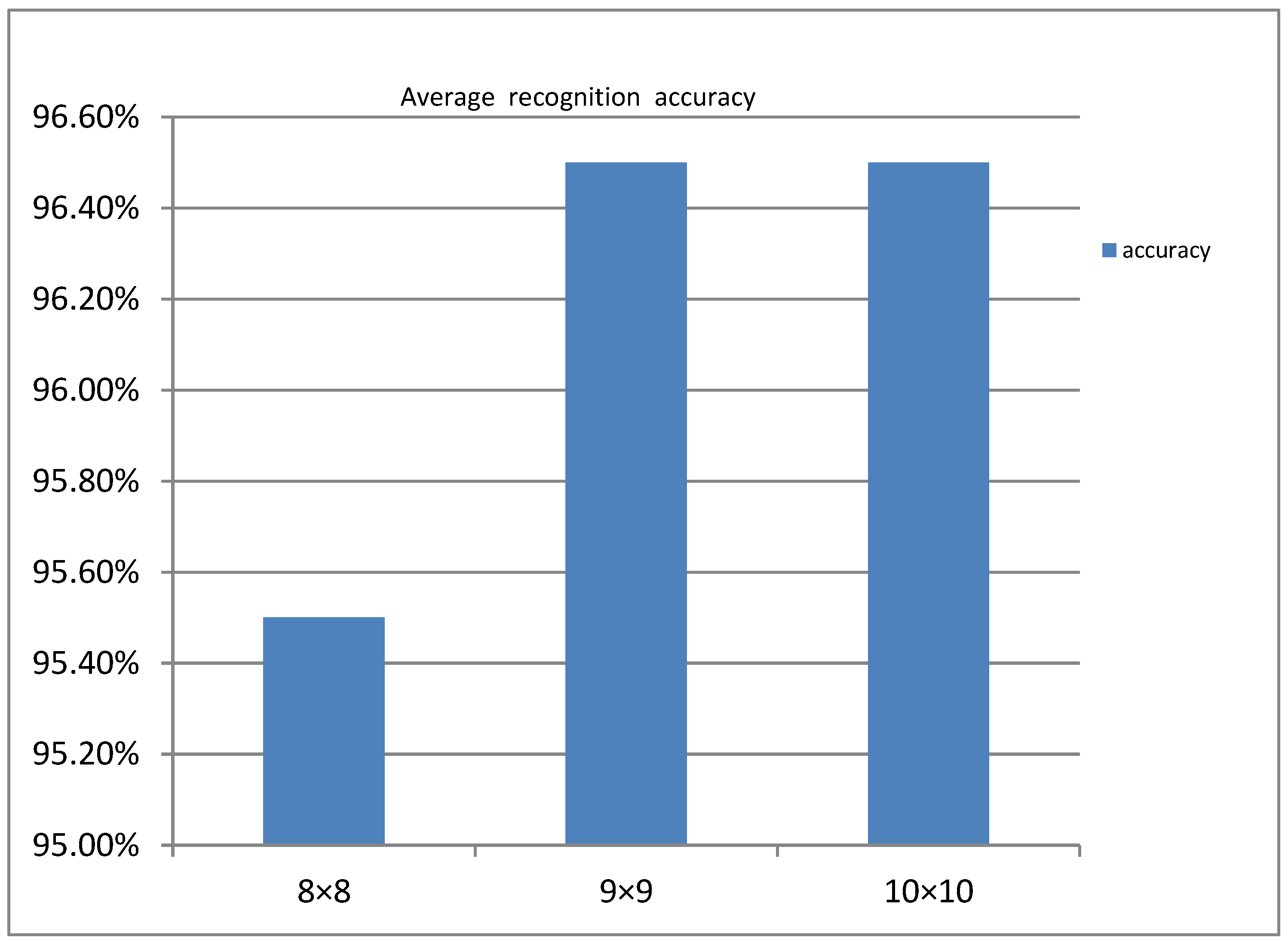
The convolution kernel size is set to 8 × 8, 9 × 9, or 10 × 10, with the convolution step set to 2. The model is then trained according to the network structure shown in Figure 6. After 3 iterations of routing and 8000 epochs. As shown in Figure 6 the relationship between the average recognition rate and the size of the convolution kernel was finally obtained.
From Figure 6, we can see that the average recognition rate when the convolution kernel size is 8 × 8 is lower than 9 × 9 and 10 × 10. However, the average recognition accuracy at 9 × 9 and 10 × 10 is not much different. For the calculation efficiency, the convolution kernel we finally chose was 9×9.
To compare CapsNet with the traditional CNN model, we used the traditional CNN model to train CT images of the liver 8000 epochs., where the CNN model selects a densely linked five-layer convolution as the control group for CapsNet.
Compared to CapsNet, the traditional CNN model’s training is relatively stable. After the number of iterations reached 2000, it basically stabilized and the training accuracy improved relatively slowly. By the end, the training accuracy had reached 87.6%. The relationship between the training accuracy of CapsNet and the number of iterations is not quite the same as that of the traditional CNN model. When CapsNet reaches 2000 iterations, the training accuracy starts to reach 90% and the loss value becomes as low as 0.2. As the number of iterations increases, the degree of oscillation gradually decreases and stabilizes. Finally, it converges to 92.9%, and the loss value eventually converges with it. Therefore, from the analysis of the variation of training accuracy in relation to the number of iterations, the use of CapsNet produced better recognition results for liver CT images.
To test and train the effect of the model on this basis, the experiment verified the accuracy of liver cancer recognition on 300 test sets and obtained two classification result tables, as shown in Table 2 and Table 3, respectively.
As can be seen from Table 2 and Table 3, CapsNet achieved an average recognition rate of 91.4% for the test set of liver CT images, which is close to the training accuracy, and improved the recall rate to around 96%. However, the traditional CNN model consisting of a densely linked five-layer convolution has an average recognition rate of only 74.6%, which differs significantly from the training results and has a recall rate of only 85%. This suggests that CapsNet has a better generalization capability than the traditional CNN model and is thus able to better recognize liver CT images.
6. Conclusions
Some characteristic information is neglected in the process of maximum pooling when using a convolutional neural network to recognize CT images. However, the capsule network’s spatial characteristics can better retain the feature information. Therefore, this paper proposes a capsule network-based method for liver cancer identification. Concurrently, we introduced a superpixel segmentation algorithm to improve the traditional NLM algorithm. To protect the information on the edge of the image better in the process of denoising the original image. Finally, the CT images of the liver were identified by a capsule network and the results were compared with a convolutional neural network. Ultimately, the CT images of the liver were identified by the capsule network and the results were compared with the convolutional neural network. In the end, the training accuracy of CT images of the liver by the capsule network and traditional CNN model reached 92.6% and 87.6%, respectively. Afterward, 300 images were randomly tested in our test set. In the end, the average recognition rates of the CapsNet and traditional CNN models were 91.4% and 74.6%, respectively, and the CapsNet improved the model recall to 95% compared to the recall rate of the traditional CNN model, which was a significant improvement. So, by comparing the test accuracy with the training accuracy, we found that CapsNet has better recognition results in the task of identifying CT images of liver cancer.
Author Contributions
Conceptualization, Q.W. and Y.X.; methodology, Q.W. and Y.X.; software, Q.W.; validation, Q.W.; formal analysis, Q.W.; investigation, Q.W. and Y.X.; resources, Q.W. and Y.X.; data curation, Q.W.; writing—original draft preparation, Q.W.; writing—review and editing, Q.W. and Y.X.; visualization, Q.W.; supervision, Y.X.; project administration, A.C.; funding acquisition, A.C. All authors have read and agreed to the published version of the manuscript.
Funding
This work was supported by Changsha Municipal & Natural Science Foundation (Grant No. kq2014160); in part by the National Natural Science Foundation in China (Grant No. 61703441); in part by the National Natural Science Foundation of Hunan Province (Grant No. 2020JJ4948); in part by the key projects of Department of Education Hunan Province (Grant No. 19A511).
Data Availability Statement
The code and data presented in this study are openly available at: https://github.com/VesperCi/Capsule-Network-for-Liver-CT-Images (accessed on 18 January 2022).
Conflicts of Interest
The authors declare no conflict of interest.
References
- Bray, F.; Ferlay, J.; Soerjomataram, I.; Siegel, R.L.; Torre, L.A.; Jemal, A. Global cancer statistics 2018: GLOBOCAN estimates of incidence and mortality worldwide for 36 cancers in 185 countries. CA A Cancer J. Clin. 2018, 68, 394–424. [Google Scholar] [CrossRef] [Green Version]
- Verma, A.; Khanna, G. A survey on digital image processing techniques for tumor detection. Indian J. Sci. Technol. 2016, 9, 15. [Google Scholar] [CrossRef]
- Anisha, P.R.; Reddy, C.K.K.; Prasad, L.V.N. A pragmatic approach for detecting liver cancer using image processing and data mining techniques; Signal processing and communication engineering systems (SPACES). In Proceedings of the 2015 International Conference on Signal Processing and Communication Engineering Systems, Guntur, India, 2–3 January 2015; pp. 352–357. [Google Scholar]
- Hu, Z.; Tang, J.; Wang, Z.; Zhang, K.; Zhang, L.; Sun, Q. Deep Learning for Image-based Cancer Detection and Diagnosis—A Survey. Pattern Recognit. 2018, 83, 134–149. [Google Scholar] [CrossRef]
- Lee, C.; Chen, S.H.; Tsai, H.M.; Chung, P.C.; Chiang, Y.C. Discrimination of liver diseases from CT images based on Gabor filters. In Proceedings of the 19th IEEE Symposium on Computer-Based Medical Systems (CBMS′06), Salt Lake City, UT, USA, 22–23 June 2006; pp. 203–206. [Google Scholar]
- Hao, T.; Zhang, Z. Texture analysis of CT images of primary liver cancer based on BP neural network. China Digit. Med. 2013, 8, 73–76. [Google Scholar]
- Liu, J.; Wang, J. Research on CT image diagnosis technology of liver cancer based on image processing. J. Tsinghua Univ. (Nat. Sci. Ed.) 2014, 54, 917–923. [Google Scholar]
- Li, W.; Jia, F.; Hu, Q. Automatic segmentation of liver tumor in CT images with deep convolutional neural networks. J. Comput. Commun. 2015, 3, 146. [Google Scholar] [CrossRef] [Green Version]
- Krishan, A.; Mittal, D. Detection and classification of liver cancer using CT images. Int. J. Recent Technol. Mech. Electr. Eng. 2015, 2, 93–98. [Google Scholar] [CrossRef]
- Li, Y.; Hao, Z.; Lei, H. Research review of convolutional neural network. Comput. Appl. 2016, 36, 2508–2515+2565. [Google Scholar]
- Luo, Y.; Zou, J.; Yao, C.; Li, T.; Bai, G. HSI-CNN: A Novel Convolution Neural Network for Hyperspectral Image. arXiv 2018, arXiv:1802.10478. [Google Scholar]
- Xi, E.; Bing, S.; Jin, Y. Capsule Network Performance on Complex Data. arXiv 2017, arXiv:1712.03480. [Google Scholar]
- Sabour, S.; Frosst, N.; Hinton, G.E. Dynamic routing between capsules. Adv. Neural Inf. Process. Syst. 2017, 30, 3856–3866. [Google Scholar]
- Yu, C.; Xiong, D. Research on finger vein recognition based on capsule network. Appl. Electron. Tech. 2018, 44, 15–18. [Google Scholar]
- Zhang, W.; Tang, P.; Zhao, L. Remote Sensing Image Scene Classification Using CNN-CapsNet. Remote Sens. 2019, 11, 494. [Google Scholar] [CrossRef] [Green Version]
- Yin, J.; Li, S.; Zhu, H.; Luo, X. Hyperspectral Image Classification Using CapsNet With Well-Initialized Shallow Layers. IEEE Geosci. Remote Sens. Lett. 2019, 16, 1095–1099. [Google Scholar] [CrossRef]
- Xiang, C.; Zhang, L.; Tang, Y.; Zou, W.; Xu, C. MS-CapsNet: A Novel Multi-Scale Capsule Network. IEEE Signal Process. Lett. 2018, 25, 1850–1854. [Google Scholar] [CrossRef]
- Wang, X.; Tan, K.; Du, Q.; Chen, Y.; Du, P. Caps-TripleGAN: GAN-Assisted CapsNet for Hyperspectral Image Classification. IEEE Trans. Geosci. Remote Sens. 2019, 57, 7232–7245. [Google Scholar] [CrossRef]
- Wang, D.; Liang, Y.; Xu, D. Capsule network for protein post-translational modification site prediction. Bioinformatics 2019, 35, 2386–2394. [Google Scholar] [CrossRef] [PubMed]
- Toraman, S.; Alakus, T.; Turkoglu, I. Convolutional capsnet: A novel artificial neural network approach to detect COVID-19 disease from X-ray images using capsule networks. Chaos Solitons Fractals 2020, 140, 110122. [Google Scholar] [CrossRef] [PubMed]
- Goceri, E. CapsNet topology to classify tumours from brain images and comparative evaluation. IET Image Process. 2020, 14, 882–889. [Google Scholar] [CrossRef]
- Chao, H.; Dong, L.; Liu, Y.; Lu, B. Emotion Recognition from Multiband EEG Signals Using CapsNet. Sensors 2019, 19, 2212. [Google Scholar] [CrossRef] [PubMed] [Green Version]
- Diwakar, M.; Kumar, M. CT image denoising using NLM and correlation-based wavelet packet thresholding. IET Image Process. 2018, 12, 708–715. [Google Scholar] [CrossRef]
- Zhu, H.; Wu, Y.; Li, P.; Wang, D.; Shi, W.; Zhang, P.; Jiao, L. A parallel Non-Local means denoising algorithm implementation with OpenMP and OpenCL on Intel Xeon Phi Coprocessor. J. Comput. Sci. 2016, 17, 591–598. [Google Scholar] [CrossRef]
- Xu, S.; Zhou, Y.; Xiang, H.; Li, S. Remote Sensing Image Denoising Using Patch Grouping-Based Nonlocal Means Algorithm. IEEE Geosci. Remote Sens. Lett. 2017, 14, 2275–2279. [Google Scholar] [CrossRef]
- Vignesh, R.; Oh, B.; Kuo, C. Fast Non-Local Means (NLM) Computation With Probabilistic Early Termination. IEEE Signal Process. Lett. 2010, 17, 277–280. [Google Scholar] [CrossRef]
- Verma, R.; Pandey, R. Grey relational analysis based adaptive smoothing parameter for non-local means image denoising. Multimed. Tools Appl. 2018, 77, 25919–25940. [Google Scholar] [CrossRef]
- Lv, J.; Luo, X. Image Denoising via Fast and Fuzzy Non-local Means Algorithm. J. Inf. Process. Syst. 2019, 15, 1108–1118. [Google Scholar]
- Luo, Y.; Huang, W.; Zeng, K.; Zhang, C.; Yu, C.; Wu, W. Intelligent Noise Reduction Algorithm to Evaluate the Correlation between Human Fat Deposits and Uterine Fibroids under Ultrasound Imaging. J. Healthc. Eng. 2021, 2021, 5390219. [Google Scholar] [CrossRef]
- Lai, R.; Yang, Y. Accelerating non-local means algorithm with random projection. Electron. Lett. 2011, 47, 182-U669. [Google Scholar] [CrossRef]
- Cheng, C.-C.; Cheng, F.-C.; Huang, S.-C.; Chen, B.-H. Integral non-local means algorithm for image noise suppression. Electron. Lett. 2015, 51, 1494-U1124. [Google Scholar] [CrossRef]
- Qian, D. Non-local mean filtering of images based on pixel selection. Foreign Electron. Meas. Technol. 2008, 37, 6–9. [Google Scholar]
- Rahim, T.; Usman, M.A.; Shin, S.Y. A survey on contemporary computer-aided tumor, polyp, and ulcer detection methods in wireless capsule endoscopy imaging. Comput. Med. Imaging Graph. 2020, 85, 101767. [Google Scholar] [CrossRef] [PubMed]
- Ning, X.; Tian, W.; He, F.; Bai, X.; Sun, L.; Li, W. Hyper-sausage coverage function neuron model and learning algorithm for image classification. Pattern Recognit. 2023, 136, 109216. [Google Scholar] [CrossRef]
- Ning, X.; Xu, S.; Nan, F.; Zeng, Q.; Wang, C.; Cai, W.; Jiang, Y. Face editing based on facial recognition features. IEEE Trans. Cogn. Dev. Syst. 2022, 1, 2379–8939. [Google Scholar] [CrossRef]
- Ning, X.; Tian, W.; Yu, Z.; Li, W.; Bai, X.; Wang, Y. HCFNN: High-order coverage function neural network for image classification. Pattern Recognit. 2022, 131, 108873. [Google Scholar] [CrossRef]
Figure 1.
Central pixel located at the edge and inside of the superpixel.

Figure 2.
Improved NLM algorithm flow chart.

Figure 3.
(A) Partial liver CT pictures before denoising; (B) Partial liver CT pictures after denoising.
Figure 3.
(A) Partial liver CT pictures before denoising; (B) Partial liver CT pictures after denoising.

Figure 4.
Image recognition process of liver cancer by CapsNet.

Figure 5.
The structure diagram of the capsule network.

Figure 6.
Average recognition rate under different convolution kernel sizes.


Table 1.
Effect of Denoise.
| a | b | c | d | |
|---|---|---|---|---|
| PSNR | 27.39 | 29.86 | 27.46 | 27.19 |
| SSIM | 93.70% | 89.51% | 94.46% | 94.96% |
Table 2.
CapsNet test results.
| Class | Samples | Identify | Precision | Recall |
|---|---|---|---|---|
| Normal | 164 | 149 | 90.8% | 95.3% |
| Cancer | 136 | 125 | 91.9% | 96.7% |
Table 3.
Traditional CNN model test results.
| Class | Samples | Identify | Precision | Recall |
|---|---|---|---|---|
| Normal | 164 | 122 | 74.3% | 84.7% |
| Cancer | 136 | 102 | 75.0% | 85.9% |
Disclaimer/Publisher’s Note: The statements, opinions and data contained in all publications are solely those of the individual author(s) and contributor(s) and not of MDPI and/or the editor(s). MDPI and/or the editor(s) disclaim responsibility for any injury to people or property resulting from any ideas, methods, instructions or products referred to in the content. |
© 2023 by the authors. Licensee MDPI, Basel, Switzerland. This article is an open access article distributed under the terms and conditions of the Creative Commons Attribution (CC BY) license (https://creativecommons.org/licenses/by/4.0/).
Share and Cite
MDPI and ACS Style
Wang, Q.; Chen, A.; Xue, Y. Liver CT Image Recognition Method Based on Capsule Network. Information 2023, 14, 183. https://doi.org/10.3390/info14030183
AMA Style
Wang Q, Chen A, Xue Y. Liver CT Image Recognition Method Based on Capsule Network. Information. 2023; 14(3):183. https://doi.org/10.3390/info14030183
Chicago/Turabian StyleWang, Qifan, Aibin Chen, and Yongfei Xue. 2023. "Liver CT Image Recognition Method Based on Capsule Network" Information 14, no. 3: 183. https://doi.org/10.3390/info14030183
Note that from the first issue of 2016, this journal uses article numbers instead of page numbers. See further details here.