An Attention-Based Deep Convolutional Neural Network for Brain Tumor and Disorder Classification and Grading in Magnetic Resonance Imaging

Abstract

This study proposes the integration of attention modules, feature-fusion blocks, and baseline convolutional neural networks for developing a robust multi-path network that leverages its multiple feature-extraction blocks for non-hierarchical mining of important medical image-related features. The network is evaluated using 10-fold cross-validation on large-scale magnetic resonance imaging datasets involving brain tumor classification, brain disorder classification, and dementia grading tasks. The Attention Feature Fusion VGG19 (AFF-VGG19) network demonstrates superiority against state-of-the-art networks and attains an accuracy of 0.9353 in distinguishing between three brain tumor classes, an accuracy of 0.9565 in distinguishing between Alzheimer’s and Parkinson’s diseases, and an accuracy of 0.9497 in grading cases of dementia.

1. Introduction

Deep learning (DL) [1] is a subset of artificial intelligence (A.I.) methods that has been gaining popularity in recent years, and it has been applied to various fields, including medical imaging, such as magnetic resonance imaging (MRI). MRI is a non-invasive imaging technique that uses a magnetic field and radio waves to produce detailed images of the body’s internal structures [2]. The technique provides high-resolution images and can diagnose a wide range of conditions.

DL algorithms have been used to improve the diagnostic accuracy and efficiency of MRI by automating the analysis of images and identifying patterns that are not visible to the human eye [3]. The algorithms can be trained to recognize specific patterns, such as tumors or abnormal brain structures, which can aid in diagnosing diseases [4].

One of the main advantages of using DL in MRI is that it can analyze large amounts of data quickly and accurately [5]. Traditional image analysis methods require manual interpretation by radiologists, which can be time-consuming and subjective. DL algorithms can be trained to analyze images, automatically saving time and improving diagnostic accuracy.

One of the main applications of DL in MRI is analyzing brain images [6]. Algorithms have been developed to detect and diagnose brain tumors, identify brain structures, and predict the progression of diseases such as Alzheimer’s [7]. This can aid in the early detection and treatment of brain diseases, leading to better patient outcomes. Another application of DL in MRI is the analysis of cardiac images [8]. Algorithms have been developed to detect and diagnose heart conditions, such as heart failure and arrhythmia. This can aid in the early detection and treatment of heart diseases.

DL algorithms have also been used to improve the diagnostic accuracy and efficiency of MRI in analyzing images of the prostate, liver, and pancreas; and to detect and diagnose prostate cancer, liver fibrosis, and pancreatic cancer [9].

One of the main challenges of using DL in MRI is the limited availability of labelled data. MRI images are often difficult to obtain and expensive to acquire, making it challenging to train DL algorithms. Additionally, the images can be of poor quality, making it difficult to detect specific patterns.

Another challenge is the variability in the MRI images. They can vary depending on the imaging protocol and the acquisition parameters. This can make it non-trivial to train generalized DL algorithms able to cope with variations in acquisition parameters.

Recent advances in the architecture and functions of convolutional neural networks (CNNs) [10] have allowed for a dramatic improvement in the performance of these models. Attention mechanisms [11] are a popular addition to CNNs, allowing for adaptive refinement of the feature maps to identify essential components of the image. Optimization strategies [12] such as batch normalization and dropout have enabled faster convergence and higher accuracy when applied to CNNs. In addition, feature fusion techniques such as sparse coding, autoencoders, and multi-resolution processing have been used to combine the strengths of multiple feature maps and have been shown to significantly improve the accuracy of CNNs.

The study proposes an innovative modification of a well-established CNN developed by the Virtual Geometry Group (VGG) [13] and named after it. We propose the integration of feature-fusion blocks and attention models to enrich the encapsulation of important image features that lead to more precise image classification. This network is employed to classify brain MRI images in brain tumor classification and brain disorder discrimination and grading.

The paper is structured as follows: In Section 2, we briefly describe the entities of DL, the attention modules, and feature-fusion blocks. The proposed network is described in detail. In addition, the employed datasets are presented. In the Section 3, the results of the study are presented. Discussion and concluding remarks take place in Section 5 and Section 6, respectively.

2. Related Work

Sadad et al. [14] utilized the Unet architecture with ResNet50 as a backbone to perform segmentation on the Figshare dataset, achieving an impressive intersection over union (IoU) score of 0.9504. The researchers also employed preprocessing and data augmentation techniques to improve classification accuracy. They used evolutionary algorithms and reinforcement learning in transfer learning to perform multi-classification of brain tumors. The study compared the performance of different DL models, such as ResNet50, DenseNet201, MobileNet V2, and InceptionV3; and demonstrated that the proposed framework outperformed the state-of-the-art methods. The study also applied various CNN models to classify brain tumors, including MobileNet V2, Inception V3, ResNet50, DenseNet201, and NASNet, achieving accuracies of 91.8%, 92.8%, 92.9%, 93.1%, and 99.6%, respectively. The NASNet model showed the highest accuracy among all the models.

Allah et al. [15] investigated the effectiveness of a novel approach to classify brain tumor MRI images using a VGG19 feature extractor and one of three different types of classifiers. To address the shortage of images needed for deep learning, the study employed a progressive, growing generative adversarial network (PGGAN) augmentation model to generate “realistic” brain tumor MRI images. The findings demonstrated that the proposed framework outperformed previous studies in accurately classifying gliomas, meningiomas, and pituitary tumors, achieving an accuracy rate of 98.54%.

In [16], a novel hybrid CNN-based architecture was proposed to classify three types of brain tumors using MRI images. The approach involves utilizing two methods of hybrid deep learning classification based on CNN. The first method combines a pre-trained Google-Net model of the CNN algorithm for feature extraction with SVM for pattern classification, while the second method integrates a finely tuned Google-Net with a soft-max classifier. The performance of the proposed approach was evaluated on a dataset containing a total of 1426 glioma images, 708 meningioma images, 930 pituitary tumor images, and 396 normal brain images. The results revealed that the finely tuned Google-Net model achieved an accuracy of 93.1%. However, the accuracy was improved to 98.1% when the Google-Net was combined with an SVM classifier as a feature extractor.

Kang et al. [17] applied transfer learning and utilized pre-trained deep convolutional neural networks to extract deep features from MRI images of the brain. These extracted features were evaluated using various machine learning classifiers, and the top three performing features were selected and combined to form an ensemble of deep features. This ensemble was then used as input to several machine learning classifiers to predict the final output. We evaluated the effectiveness of different pre-trained models as deep feature extractors, various machine learning classifiers, and the impact of the ensemble of deep features for brain tumor classification using three openly accessible brain MRI datasets. The experimental results revealed that using an ensemble of deep features significantly improved performance, and SVM with radial basis function kernel outperformed other machine learning classifiers, particularly for large datasets.

Sivaranjini et al. [18] used a DL neural network to classify MRI images of healthy individuals and those with Parkinson’s disease (PD). The researchers utilized the AlexNet convolutional neural network architecture to improve the accuracy of Parkinson’s disease diagnosis. By training the network with MRI images and testing it, the system was able to achieve an accuracy rate of 88.9%. This demonstrates that deep learning models can aid clinicians in diagnosing PD more objectively and accurately in the future.

Bhan et al. [19] successfully diagnosed PD from MRI images. The LeNet-5 architecture and a dropout algorithm achieved 97.92% accuracy using batch normalization on a large dataset consisting of 10,548 images. This method has the potential to accurately diagnose various stages of PD.

Hussain et al. [20] presented a 12-layer CNN for binary classification and detection of Alzheimer’s disease using brain MRI data. The proposed model’s performance is evaluated and compared to existing CNN models based on accuracy, precision, recall, F1 score, and receiver operating characteristic (ROC) curve using the open access series of imaging studies (OASIS) dataset. The model attained an accuracy of 97.75%, higher than any previously published CNN models on this dataset.

Salehi et al. [21] used to detect and classify Alzheimer’s Disease (AD) at an early stage by analyzing MRI images from the ADNI database. The dataset consisted of 1512 mild, 2633 normal, and 2480 AD images. The CNN model achieved a remarkable accuracy of 99%, surpassing the performance of several other studies.

3. Materials and Methods

3.1. Deep Learning

DL is a branch of machine learning that uses neural networks with many layers to learn patterns and features from data [10]. It is based on the idea that a neural network can learn to recognize data patterns like a human brain does [1].

DL algorithms comprise multiple layers of artificial neural networks, interconnected layers of nodes, or artificial neurons. These layers work together to extract features from the data and make predictions. The first layer of a DL network is typically responsible for recognizing simple features, such as edges or shapes, while the last layer makes the final prediction.

DL networks are trained using large amounts of data, fed into the network, and used to adjust the weights and biases of the artificial neurons. The goal is to adjust these weights and biases, so the network can correctly classify or predict the output for new input data. This process is known as supervised learning, where the network is trained on labelled data [22].

DL networks are also used in unsupervised learning, where the network is not provided with labelled data and has to find patterns and features on its own. This can be useful for image compression, anomaly detection, and generative models.

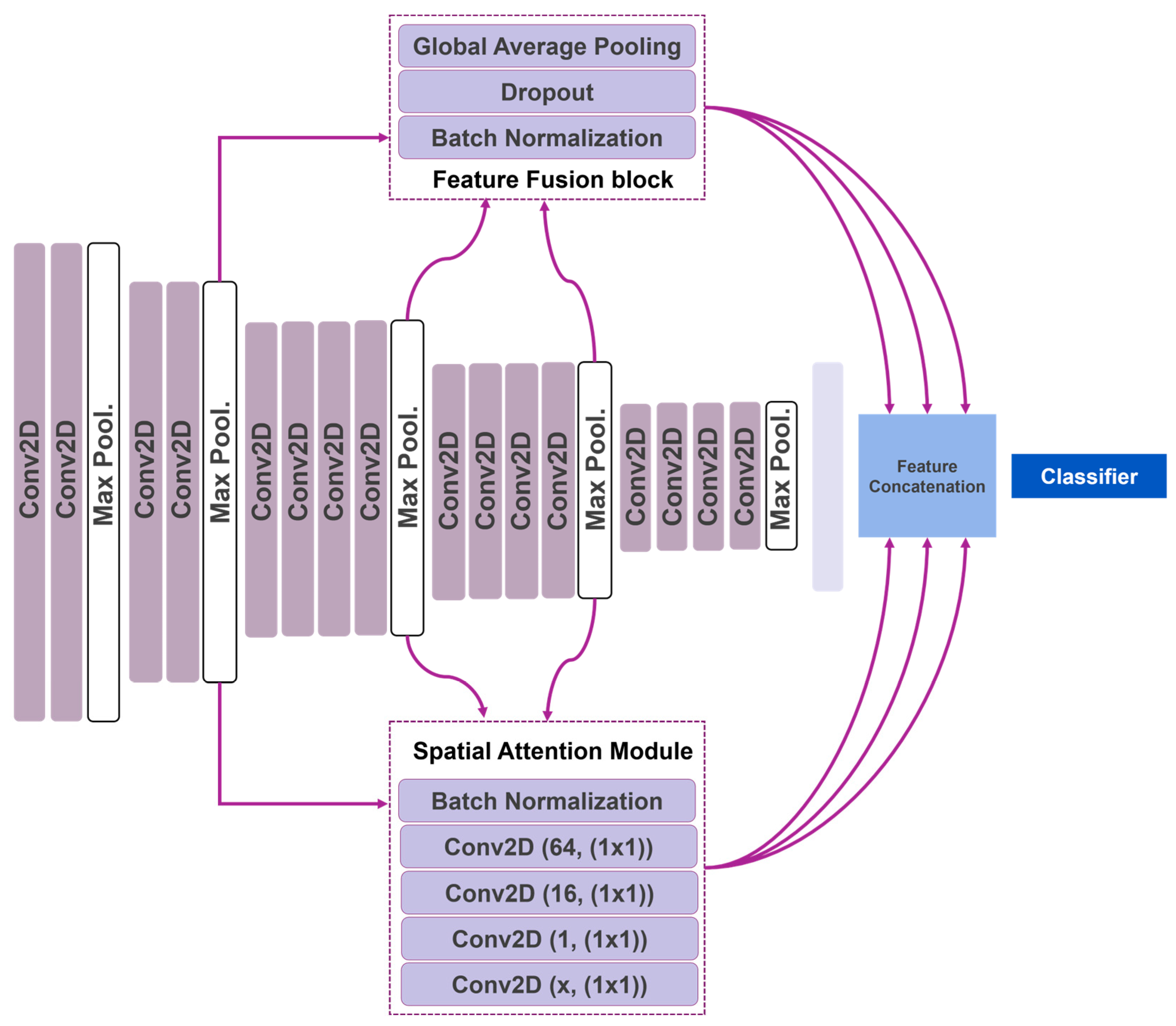
3.2. Attention Feature-Fusion VGG19

The study proposes an innovative expansion of the baseline VGG19 network. It circumvents the baseline’s hierarchical feature extraction method using handcrafted feature fusion blocks and feature concatenation. The latter modification led to the creation of the Feature-Fusion VGG19 network [23]. Here, we propose an extension of this network that leverages the attention modules. The components of the Attention Feature-Fusion VGG19 (AFF-VGG19) network are analytically described below.

3.2.1. Virtual Geometry Group

VGG19 is a CNN architecture developed by the Visual Geometry Group (VGG) at the University of Oxford in 2014 [13]. It is a deeper version of the VGG16 architecture known for its excellent performance in image classification tasks.

The VGG19 network architecture comprises 19 layers, including 16 convolutional layers and three fully connected layers. The convolutional layers extract features from the input image, while the fully connected layers are used for classification. The architecture uses a small 3 × 3 convolutional kernel size, which allows for a deeper architecture with more layers.

One of the critical features of the VGG19 architecture is its use of tiny convolutional filters, which allows the network to learn more fine-grained features from the input image [13]. Additionally, the network uses many filters in each convolutional layer, which allows it to learn many features from the input image.

The VGG19 network was trained on the ImageNet dataset, a large dataset of images labelled with one of 1000 different classes. The network was trained using the stochastic gradient descent (SGD) optimization algorithm with a batch size of 128 and a learning rate of 0.001.

The VGG19 network achieved state-of-the-art performance on the ImageNet dataset [24], with an accuracy of 92.7% on the validation set. This made it one of the most accurate CNNs at its release, and it is still considered a very accurate network today.

Training VGG19 from scratch involves learning 143 million parameters, a colossal number for small-scale datasets. Supplying such a network with inadequate amounts of data results in underfitting. Therefore, we considered the fine-tuning option, which borrows the architecture and some pre-assigned conditions to reduce the number of trainable parameters. The initial network training defined the untrainable weights, which were defined using the ImageNet database [24]. Though the latter dataset consists of irrelevant images (non-medical), successful training helps the network learn how to extract low-level image features (e.g., edges, shapes), which are met in medical images also. Therefore, it is fair to transfer this knowledge to other domains [25,26,27].

We propose that the VGG19 network of the study is fine-tuned to extract approximately 5 million trainable parameters to circumvent underfitting. We selected to train the deep convolutional layers and freeze the first ones because abstract and high-level features are learned from the deeper convolutional layers of the network.

3.2.2. Feature Fusion Modification

Feature fusion is a modification to the traditional CNN architecture that allows for extracting features from an input image in a non-hierarchical way. This modification is used to improve the performance of CNNs in tasks, such as image classification, object detection, and semantic segmentation.

In traditional CNNs, features are extracted hierarchically. Lower-level features are learned in the earlier layers, and higher-level features are learned in the later layers. However, feature fusion CNNs extract features from multiple layers simultaneously and combine to form a single set of features. This allows for extracting low-level and high-level features in a non-hierarchical way.

There are several different ways to implement feature fusion in a CNN. One standard method combines different layers, such as convolutional layers, pooling layers, and fully connected layers. These layers are trained to extract features from the input image at different levels of abstraction. The features from each layer are then combined to form a single set of features.

Another method is to use feature pyramid networks (FPN), which combines features from different layers of a CNN in a pyramid-like structure. This allows for the extraction of features at different scales, which can be helpful in tasks such as object detection, where the size of the object can vary greatly.

A third method is to use an attention-based feature fusion technique, which uses an attention mechanism to selectively focus on different regions of the input image when extracting features. This allows the network to pay more attention to the regions of the image that are most important for the task at hand.

We propose using simple feature-fusion blocks that solely connect the output of the convolutional blocks directly to the top of the network (Figure 1). A feature-fusion block involves a batch normalization, dropout, and global average pooling layers. These layers do not extract additional features. The feature-fusion blocks are placed after the second, third, and fourth convolutional groups and are connected to the output of the max pooling layers that follow (Figure 1). In this way, the extorted image features of each convolutional group are connected directly to the classification layer at the top of the network, ensuring that no further processing is applied. Therefore, the feature-fusion blocks negate the hierarchical feature-extraction manner of the VGG19.

3.2.3. Attention Mechanism

The attention mechanism is a technique used in convolutional neural networks (CNNs) to focus on the essential parts of an image when making predictions. It allows the network to selectively attend to different regions of the input image rather than treating the entire image as a single input.

The attention mechanism is typically implemented as an additional layer in the CNN, which is trained to learn the importance of different input image regions. This layer is often referred to as the attention layer. The attention layer is trained to learn a weighting for each region of the input image, which is used to determine the importance of that region when making predictions.

There are different attention mechanisms, but one of the most widely used is the “soft attention” mechanism. It is a different form of attention, which means it can be trained with backpropagation. This is accomplished by computing a set of attention weights for each region of the input image and then using these weights to weight the contributions of each region to the final prediction.

The attention mechanism can be applied differently in CNNs depending on the task. For instance, in image captioning, attention can focus selectively on different regions of an image when generating a text description of the image. In image classification, attention can be used to focus on specific regions of an image that are most relevant to the class of interest.

We propose using five-layered attention modules located after the second, third, and fourth convolutional groups and connected to the output of the following max pooling layers. The first layer is a batch normalization layer. The second, third, fourth, and fifth layers are convolutional operations utilizing 64, 16, 1, and x filters of 1 × 1 kernel size. The x number depends on the convolution group to which the attention module belongs. The attention module in the second group has an x of 128. Accordingly, the third and fourth groups have an x of 256 and 512, respectively. The extracted features are multiplied with the output of the convolutional group and connected to the network’s top.

3.3. Datasets of the Study

The study enrols three classification datasets derived from four repositories, as presented in

Table 1. Study’s datasets overview.

Dataset	Source (s)	Number of Images
Brain Tumors Dataset	https://www.kaggle.com/datasets/adityakomaravolu/brain-tumor-mri-images (accessed on 24 November 2022). https://www.kaggle.com/datasets/roroyaseen/brain-tumor-data-mri (accessed on 24 November 2022).	7023 and 19,226. Total 26,249
Brain Disorders Dataset	https://www.kaggle.com/datasets/farjanakabirsamanta/alzheimer-diseases-3-class (accessed on 24 November 2022).	7756
Dementia Grading Dataset	https://www.kaggle.com/datasets/sachinkumar413/alzheimer-mri-dataset (accessed on 24 November 2022).	6400

.

3.3.1. Brain Tumors Dataset

Glioma is a type of brain tumor that arises from glial cells, which are the supporting cells of the nervous system [28]. They can be benign or malignant, and the malignant forms can be very aggressive. Symptoms can include headaches, seizures, and changes in cognitive function. Meningioma is a type of brain tumor arising from the meninges, the protective membranes covering the brain, and spinal cord [28]. They are generally benign tumors, but can cause symptoms such as headaches, seizures, and changes in cognitive function. Pituitary tumors develop in the pituitary gland, a small gland located at the base of the brain that produces hormones that regulate growth, metabolism, and other bodily functions [28]. Pituitary tumors can be benign or malignant and can cause symptoms such as headaches, vision problems, and changes in hormone levels.

In the present study, the final brain tumors dataset combines two publicly available datasets (Table 1). The datasets contain MRI images of glioma (8208 images), meningioma (7866 images), pituitary tumors (8175 images), and controls (2000). Henceforth, the classes are addressed as follows: glioma (G), meningioma (M), and pituitary (P).

The images are preprocessed and converted into JPEG format. The dataset is suitable for training DL networks for discriminating the classes.

3.3.2. Brain Disorders Dataset

AD is a progressive brain disorder that affects memory, thinking and behavior [29]. It is the most common cause of dementia, a general term for a decline in cognitive function severe enough to interfere with daily life. AD symptoms typically develop slowly and worsen over time, eventually leading to severe cognitive impairment and the inability to carry out daily activities [29]. The cause of AD is not fully understood. However, it is thought to be related to genetic, lifestyle, and environmental factors.

PD is a progressive nervous system disorder that affects movement [29]. It is caused by the loss of dopamine-producing cells in the brain, leading to symptoms such as tremors, stiffness, slow movement, and difficulty with balance and coordination. Parkinson’s disease can also cause non-motor symptoms such as depression, anxiety, and cognitive impairment. The cause of PD is not fully understood. However, it involves a combination of genetic and environmental factors. There is no cure for PD, but medications and other treatments can help manage symptoms.

The study’s dataset contains 7756 MRI images separated into three classes: PD with 906 images, AD with 3200 images, and controls with 3650 images. All the images are 176 × 208 pixels in size and come in JPEG format. This dataset is used to teach the network to distinguish between these classes.

3.3.3. Dementia Grading Dataset

Dementia is a general term for a decline in cognitive function severe enough to interfere with daily life. The severity of dementia can be graded or classified in various ways, but the most widely used system is the clinical dementia rating (CDR) scale [30,31]. The CDR scale ranges from 0 to 3, with 0 indicating no dementia, 1 indicating very mild dementia, 2 indicating mild dementia, and 3 indicating moderate to severe dementia.

The CDR scale assesses six areas of cognitive function: memory, orientation, judgment and problem solving, community affairs, home and hobbies, and personal care. The score in each area is used to determine the overall CDR score.

The CDR scale is a widely used and accepted tool for evaluating the severity of dementia and tracking its progression over time. Other scales used to grade dementia are the global deterioration scale (GDS) and the global clinical impression of change (GCIC).

It is important to note that while grading or classifying the severity of dementia can be helpful for research and tracking the progression of the disease, it is not always a definitive measure of an individual’s cognitive or functional abilities.

The dataset of the particular study is collected from several websites/hospitals/public repositories and consists of MRI images of 128 × 128 pixel size. The total number of images is 6400. The distribution between classes is as follows: mildly demented (896 images), moderately demented (64 images), non-demented (3200 images), and very mildly demented (2240 images). Henceforth, the above classes are addressed as: mildly demented (Mi), moderately demented (Mo), and very mildly demented (VMi).

The images are preprocessed and converted into JPEG format.

3.4. Experiment Setup

The experiments were conducted on a workstation featuring an 11th Gen Intel® Core™ i9-11900KF @3.50GHz processor, an NVIDIA GeForce RTX 3080 Ti GPU and 64 GB of RAM, running a 64-bit operating system. Tensorflow 2.9.0 and Sklearn 1.0.2 were used during the experiments, both written in Python 3.9.

The assessment of the models was conducted using 10-fold cross-validation. During each fold, the accuracy (ACC), sensitivity (SEN), specificity (SPE), positive predicted value (PPV), negative predicting value (NPV), false positive rate (FPR), false negative rate (FNR), F-1 score (F1) of the run were calculated based on the recorded true positives (T.P.), false positives (FP), true negatives (TN), and false negatives (FN) of each class. In addition, from the predicted probabilities, we computed the area under curve score (AUC).

4. Results

Section 4.1 describes the classification performance of the AFF-VGG19 network on the brain tumor dataset. Section 4.2. presents the results of the network when classifying the brain disorders dataset. Accordingly, in Section 4.3., the performance of AFF-VGG19 in the dementia grading dataset is presented. Finally, Section 4.4. presents comparisons between the proposed AFF-VGG19 network and alternative state-of-the-art networks.

4.1. Brain Tumor Classification

The proposed network achieves an aggregated accuracy of 0.9353, computed based on the total true positives between the classes. The model shows excellent performance in distinguishing between tumor and non-tumor MRI images. Specifically, the network exhibits an accuracy of 0.9795 in the control class, with a very small FPR (0.0219), as

Table 2. Performance metrics of AFF-VGG19 on the brain tumor dataset. G stands for glioma, M for meningioma, P for pituitary.

	ACC	SEN	SPE	PPV	NPV	FPR	FNR	F1	AUC
G	0.9505	0.9676	0.9427	0.8849	0.9846	0.0573	0.0324	0.9244	0.9552
M	0.9304	0.9062	0.9408	0.8675	0.9591	0.0592	0.0938	0.8864	0.9235
P	0.9572	0.9161	0.9758	0.9449	0.9626	0.0242	0.0839	0.9303	0.9460
Control	0.9795	0.9960	0.9781	0.7895	0.9997	0.0219	0.0040	0.8808	0.9871

presents.

For the G class, the network achieves an accuracy of 0.9505, a sensitivity of 0.9676, and a specificity of 0.9427. The AUC score reaches 0.9552. For the M class, the network achieves an accuracy of 0.9304, a sensitivity of 0.9062, and a specificity of 0.9408. The AUC score reaches 0.9235. Accordingly, for the P class, the network achieves an accuracy of 0.9572, a sensitivity of 0.9161, and a specificity of 0.9758. The AUC score reaches 0.9460.

The relatively large FNR (0.0938) and accuracy (0.9304) in the M class indicate that the network performs sub-optimally in the discrimination of the M class from the rest (M versus ALL classification).

4.2. Brain Disorders Classification

AFF-VGG19 achieves an aggregated accuracy of 0.9565. The model shows excellent performance in distinguishing between AD-PD and control MRI images. Specifically, the network exhibits an accuracy of 0.9621 in the control class, with a very small FPR (0.0375), as

Table 3. Performance metrics of AFF-VGG19 on the brain disorders dataset. AD stands for Alzheimer’s disease and PD for Parkinson’s disease.

	ACC	SEN	SPE	PPV	NPV	FPR	FNR	F1	AUC
AD	0.9409	0.9222	0.9541	0.9339	0.9458	0.0459	0.0778	0.9280	0.9382
PD	0.9489	0.9860	0.9160	0.9125	0.9866	0.0840	0.0140	0.9479	0.9510
Control	0.9621	0.9592	0.9625	0.7718	0.9944	0.0375	0.0408	0.8553	0.9608

presents.

For the AD class, the network achieves an accuracy of 0.9409, a sensitivity of 0.9222, and a specificity of 0.9541. The AUC score reaches 0.9382. For the PD class, the network achieves an accuracy of 0.9489, a sensitivity of 0.9860, and a specificity of 0.9160. The AUC score reaches 0.9510.

AFF-VGG19 yields a relatively high FPR in PD detection and a larger FNR in AD detection (0.0840 and 0.0778, respectively).

4.3. Dementia Grading

AFF-VGG19 achieves an aggregated accuracy of 0.9497. The model shows excellent performance in distinguishing between Mo-Mi-VMi and control MRI images. Specifically, the network exhibits an accuracy of 0.9769 in the control class, with a very small FPR (0.0394), as

Table 4. Performance metrics of AFF-VGG19 on the dementia grading dataset. Mo stands for moderate, Mi for mild, and VMi for very mild.

	ACC	SEN	SPE	PPV	NPV	FPR	FNR	F1	AUC
Mo	0.9670	0.9531	0.9672	0.2268	0.9995	0.0328	0.0469	0.3664	0.9601
Mi	0.9264	0.8281	0.9424	0.7007	0.9712	0.0576	0.1719	0.7591	0.8853
VMi	0.9539	0.9362	0.9635	0.9324	0.9656	0.0365	0.0638	0.9343	0.9498
Control	0.9769	0.9931	0.9606	0.9619	0.9929	0.0394	0.0069	0.9772	0.9769

presents. In addition, a very low FNR is recorded (0.0069).

For the Mo class, the network achieves an accuracy of 0.9670, a sensitivity of 0.9531, and a specificity of 0.9672. The AUC score reaches 0.9601. For the Mi class, the network achieves an accuracy of 0.9264, a sensitivity of 0.8281, and a specificity of 0.9424. The AUC score reaches 0.8853. For the VMi class, the network yields an accuracy of 0.9539, a sensitivity of 0.9362, a specificity of 0.9635, and an AUC of 0.9498.

Figure 2 summarizes the performance of AFF-VGG19. Figure 2 presents the ROC curve, and the training and validation accuracy and loss for the brain tumor and brain disorder datasets.

4.4. Comparison with The State-Of-The-Art

AFF-VGG19 obtains the highest aggregated accuracy in every dataset (

Table 5. Accuracy of 17 state-of-the-art networks on the three datasets of the study.

	Brain Tumor	Brain Disorder	Dementia Grading
Xception	0.8850	0.8925	0.8786
VGG16	0.8897	0.8704	0.9088
VGG19	0.9108	0.8981	0.9022
ResNet152	0.8600	0.8646	0.8983
ResNet152V2	0.8801	0.8613	0.8984
InceptionV3	0.8713	0.8657	0.8961
InceptionResNetV2	0.8848	0.8605	0.8872
MobileNet	0.8689	0.8511	0.9091
MobileNetV2	0.8512	0.8312	0.9150
DenseNet169	0.8732	0.8442	0.9066
DenseNet201	0.8715	0.8495	0.8891
NASNetMobile	0.8594	0.8695	0.9011
EfficientNetB6	0.8734	0.8726	0.8975
EfficientNetB7	0.8606	0.8717	0.8892
EfficientNetV2B3	0.8804	0.8693	0.8814
ConvNeXtLarge	0.8732	0.8463	0.9095
ConvNeXtXLarge	0.8702	0.8422	0.8898
ATT-FF-VGG19	0.9353	0.9565	0.9497

) compared to state-of-the-art CNNs, which do not use attention modules. In addition, the baseline VGG19 network stands out among its competitors when comparing non-attention-based models. Specifically, VGG19 exhibits the best accuracy in the brain tumor dataset (accuracy of 0.9108), the best accuracy in the brain disorder dataset (accuracy of 0.8981), and the fourth-best accuracy in the dementia grading dataset (accuracy of 0.9022).

The results of Table 5 justify the selection of the baseline VGG19 as the main component for an attention-based feature-fusion network.

The study compares the proposed method and methods presented by recent related works on similar datasets.

Table 6. Comparisons with related research.

First Author	Ref. No.	Test Data Size	Classes	Method	ACC	SEN	SPE
Sadad	[14]	612 slices	G-M-P	NASNet	0.996	-	-
Allah	[15]	460 slices	G-M-P	VGG19	G: 0.9854 M: 0.9857 P: 1	G: 0.9777 M: 0.9804 P: 1	G: 0.9914 M: 0.9871 P: 1
Rasool	[16]	692 slices	G-M-P-controls	Google-Net	0.981	G: 0.978 M: 0.973 P: 0.989 N: 0.987
Kang	[17]	692 slices		DenseNet-169	0.9204	-	-
This study		26,249 slices	G-M-P-controls	AFF-VGG19	G: 0.9505 M: 0.9304 P: 0.9572	G: 9676 M: 0.9062 P: 0.9161	G: 0.9427 M: 0.9062 P: 0.9758
Bhan	[19]	1055 Slices	PD-controls	LeNet-5	0.9792	-	-
Sivaranjini	[18]	36 patients	PD-controls	AlexNet	0.889	-	-
Hussain	[20]	11 patients	AD-controls	CNN	0.9775	AD: 0.92 C: 1	-
This study		7756 slices	PD-AD-controls	AFF-VGG19	PD: 0.9409 AD: 0.9489	PD: 0.9222 AD: 0.9860	PD: 0.9541 AD: 0.9160
Salehi	[21]	7635 slices	Mi-VMi-controls	CNN	0.99	-	-
Mohammed	[32]	6400 slices	Mi-VMi-Mo-controls	AlexNet	94.8	93	97.75
This study		6400 slices	Mi-VMi-Mo-controls	AFF-VGG19	Mo: 0.967 Mi: 0.9264 VMi: 0.9539	Mo: 0.9531 Mi: 0.8281 VMi: 0.9362	Mo: 0.9672 Mi: 0.9424 VMi: 0.9635

summarizes the results.

Compared to recent literature, the present study utilized large-scale data (brain tumor and brain disorders datasets). Still, the results are consistent with the literature and verify that the proposed methodology is robust for big-data classification.

4.5. Reproducibility

This section presents the results of statistical significance tests to verify the reproducibility of the experiments and the stability of the proposed approach. For this purpose, AFF-VGG19 was trained and validated under a 10-fold cross-validation on each dataset 20 times, and a T-test was performed. The results verify that the model produces consistent outcomes without statistically significant deviations from the initially reported accuracy (

Table 7. Statistical significance test results.

	Brain Tumor	Brain Disorder	Dementia Grading
Mean	0.9355	0.9558	0.9491
Standard Deviation	0.002	0.002	0.001
t-statistic	0.4	−1.09	−1.9
Null Hypothesis	Mean = 0.9355	Mean = 0.9565	Mean = 0.9497
Result	At the 0.05 level, the population mean is NOT significantly different from the test mean (0.9353).	At the 0.05 level, the population mean is NOT significantly different from the test mean (0.9565).	At the 0.05 level, the population mean is NOT significantly different from the test mean (0.9497).

).

5. Discussion

DL will likely play an important role in disease diagnosis and classification from MRI images. With the ability to detect subtle changes in MRI images, accurately diagnose and classify diseases, detect and segment lesions, identify biomarkers, develop personalized medicine, and develop new diagnostic tools and therapies, deep learning has the potential to revolutionize medical imaging and improve patient outcomes.

The study proposed a modification of the baseline VGG19 network that improves its feature-extraction capabilities. Integrating the feature-fusion block and attention module avoided the hierarchical nature of the baseline model and improved the classification accuracy. The model was evaluated using three MRI datasets related to brain tumor discrimination, brain disorder classification, and dementia grading. The AFF-VGG19 network demonstrates superiority against state-of-the-art networks. It attains an accuracy of 0.9353 in distinguishing between three brain tumor classes, an accuracy of 0.9565 in distinguishing between AD and PD, and an accuracy of 0.9497 in grading cases of dementia. The high FPR in PD detection and high FNR in AD detection may have their cause in the fact that these two classes may give similar findings and patterns in specific parts of the image, such that they confuse the model as there are no distinct differences. For this purpose, it would be useful in future research to also consider clinical data that would probably help to better and more accurately determine the image classes.

Without integrating the attention and feature-fusion blocks, the baseline VGG19 network proved superior to the rest of the pretrained networks (Table 5). Therefore, the attention and feature-fusion blocks were implemented using the baseline VGG19 architecture as the main feature-extraction pipeline.

The study has limitations that the authors aim to tackle in the future. Firstly, the proposed network needs further evaluation using more MRI datasets to verify its effectiveness. Secondly, more fine-tuning and hyper-parameter tuning may be required depending on the particular dataset and classification task. In the present study, the same parameters were used for each dataset, which may decrease the efficiency. Thirdly, the attention modules can be further improved and attached to other state-of-the-art networks.

A CNN can be trained to identify features such as edges, textures, and shapes in an image associated with a particular disease or abnormality. By visualizing the intermediate representations of the network, medical experts can gain insights into which features the network is using to make its predictions. This can help to validate the network’s predictions and provide additional information that can be used to support medical decision-making. In this context, the lack of post-hoc explainability-enhancing algorithms in the present study is a limitation and an opportunity for future studies.

Nevertheless, the proposed network achieves a top accuracy in every task. It proves to be superior to the baseline VGG19 model and other pretrained networks.

6. Conclusions

Recent advances in the architecture and functions of CNNs have allowed for a dramatic improvement in the performance of these models. The study proposes an innovative modification of VGG19 with integration of feature-fusion blocks and attention models to enrich the encapsulation of important image features that lead to more precise image classification. The AFF-VGG19 network demonstrated obtained an accuracy of 0.9353 in distinguishing between three brain tumor classes, an accuracy of 0.9565 in distinguishing between AD and PD, and an accuracy of 0.9497 in grading cases of dementia from MRI images. Future research should focus on evaluating the network using more datasets, enhancing the explainability of the framework, and tuning the attention modules to obtain more precise results.

References

1. Goodfellow, I.; Bengio, Y.; Courville, A.; Bengio, Y. Deep Learning; MIT Press: Cambridge, MA, USA, 2016; Volume 1. [Google Scholar]
2. Plewes, D.B.; Kucharczyk, W. Physics of MRI: A Primer. J. Magn. Reson. Imaging 2012, 35, 1038–1054. [Google Scholar] [CrossRef]
3. Lundervold, A.S.; Lundervold, A. An Overview of Deep Learning in Medical Imaging Focusing on MRI. Z. Med. Phys. 2019, 29, 102–127. [Google Scholar] [CrossRef] [PubMed]
4. Turkbey, B.; Haider, M.A. Deep Learning-Based Artificial Intelligence Applications in Prostate MRI: Brief Summary. Br. J. Radiol. BJR 2022, 95, 20210563. [Google Scholar] [CrossRef] [PubMed]
5. Noor, M.B.T.; Zenia, N.Z.; Kaiser, M.S.; Mamun, S.A.; Mahmud, M. Application of Deep Learning in Detecting Neurological Disorders from Magnetic Resonance Images: A Survey on the Detection of Alzheimer’s Disease, Parkinson’s Disease and Schizophrenia. Brain Inf. 2020, 7, 11. [Google Scholar] [CrossRef] [PubMed]
6. Mostapha, M.; Styner, M. Role of Deep Learning in Infant Brain MRI Analysis. Magn. Reson. Imaging 2019, 64, 171–189. [Google Scholar] [CrossRef]
7. Akkus, Z.; Galimzianova, A.; Hoogi, A.; Rubin, D.L.; Erickson, B.J. Deep Learning for Brain MRI Segmentation: State of the Art and Future Directions. J. Digit. Imaging 2017, 30, 449–459. [Google Scholar] [CrossRef] [Green Version]
8. Tao, Q.; Lelieveldt, B.P.F.; van der Geest, R.J. Deep Learning for Quantitative Cardiac MRI. Am. J. Roentgenol. 2020, 214, 529–535. [Google Scholar] [CrossRef]
9. Schelb, P.; Kohl, S.; Radtke, J.P.; Wiesenfarth, M.; Kickingereder, P.; Bickelhaupt, S.; Kuder, T.A.; Stenzinger, A.; Hohenfellner, M.; Schlemmer, H.-P.; et al. Classification of Cancer at Prostate MRI: Deep Learning versus Clinical PI-RADS Assessment. Radiology 2019, 293, 607–617. [Google Scholar] [CrossRef] [Green Version]
10. LeCun, Y.; Bengio, Y.; Hinton, G. Deep learning. Nature 2015, 521, 436–444. [Google Scholar] [CrossRef]
11. Vaswani, A.; Shazeer, N.; Parmar, N.; Uszkoreit, J.; Jones, L.; Gomez, A.N.; Kaiser, L.; Polosukhin, I. Attention Is All You Need. arXiv 2017. [Google Scholar] [CrossRef]
12. Le, Q.V.; Ngiam, J.; Coates, A.; Lahiri, A.; Prochnow, B.; Ng, A.Y. On optimization methods for deep learning. In Proceedings of the ICML, Bellevue, WA, USA, 28 June–2 July 2011. [Google Scholar]
13. Simonyan, K.; Zisserman, A. Very Deep Convolutional Networks for Large-Scale Image Recognition. arXiv 2015, arXiv:1409.1556. [Google Scholar]
14. Sadad, T.; Rehman, A.; Munir, A.; Saba, T.; Tariq, U.; Ayesha, N.; Abbasi, R. Brain tumor detection and multi-classification using advanced deep learning techniques. Microsc. Res. Tech. 2021, 84, 1296–1308. [Google Scholar] [CrossRef]
15. Gab Allah, A.M.; Sarhan, A.M.; Elshennawy, N.M. Classification of Brain MRI Tumor Images Based on Deep Learning PGGAN Augmentation. Diagnostics 2021, 11, 2343. [Google Scholar] [CrossRef] [PubMed]
16. Rasool, M.; Ismail, N.A.; Boulila, W.; Ammar, A.; Samma, H.; Yafooz, W.M.S.; Emara, A.-H.M. A Hybrid Deep Learning Model for Brain Tumour Classification. Entropy 2022, 24, 799. [Google Scholar] [CrossRef] [PubMed]
17. Kang, J.; Ullah, Z.; Gwak, J. MRI-Based Brain Tumor Classification Using Ensemble of Deep Features and Machine Learning Classifiers. Sensors 2021, 21, 2222. [Google Scholar] [CrossRef] [PubMed]
18. Sivaranjini, S.; Sujatha, C.M. Deep learning based diagnosis of Parkinson’s disease using convolutional neural network. Multimed. Tools Appl. 2020, 79, 15467–15479. [Google Scholar] [CrossRef]
19. Bhan, A.; Kapoor, S.; Gulati, M.; Goyal, A. Early Diagnosis of Parkinson’s Disease in brain MRI using Deep Learning Algorithm. In Proceedings of the 2021 Third International Conference on Intelligent Communication Technologies and Virtual Mobile Networks (ICICV), Tirunelveli, India, 4–6 February 2021; IEEE: Tirunelveli, India, 2021; pp. 1467–1470. [Google Scholar]
20. Hussain, E.; Hasan, M.; Hassan, S.Z.; Hassan Azmi, T.; Rahman, M.A.; Zavid Parvez, M. Deep Learning Based Binary Classification for Alzheimer’s Disease Detection using Brain MRI Images. In Proceedings of the 2020 15th IEEE Conference on Industrial Electronics and Applications (ICIEA), Kristiansand, Norway, 9–13 November 2020; IEEE: Kristiansand, Norway, 2020; pp. 1115–1120. [Google Scholar]
21. Salehi, A.W.; Baglat, P.; Sharma, B.B.; Gupta, G.; Upadhya, A. A CNN Model: Earlier Diagnosis and Classification of Alzheimer Disease using MRI. In Proceedings of the 2020 International Conference on Smart Electronics and Communication (ICOSEC), Trichy, India, 10–12 September 2020; IEEE: Trichy, India, 2020; pp. 156–161. [Google Scholar]
22. Alloghani, M.; Al-Jumeily, D.; Mustafina, J.; Hussain, A.; Aljaaf, A.J. A Systematic Review on Supervised and Unsupervised Machine Learning Algorithms for Data Science. In Supervised and Unsupervised Learning for Data Science; Unsupervised and Semi-Supervised Learning; Berry, M.W., Mohamed, A., Yap, B.W., Eds.; Springer International Publishing: Cham, Switzerland, 2020; pp. 3–21. ISBN 978-3-030-22474-5. [Google Scholar]
23. Apostolopoulos, I.D.; Papathanasiou, N.D. Classification of lung nodule malignancy in computed tomography imaging utilizing generative adversarial networks and semi-supervised transfer learning. Biocybern. Biomed. Eng. 2021, 41, 1243–1257. [Google Scholar] [CrossRef]
24. Deng, J.; Dong, W.; Socher, R.; Li, L.-J.; Li, K.; Fei-Fei, L. Imagenet: A large-scale hierarchical image database. In Proceedings of the 2009 IEEE Conference on Computer Vision and Pattern Recognition, Miami, FL, USA, 20–25 June 2009; IEEE: New York, NY, USA; pp. 248–255. [Google Scholar]
25. Huh, M.; Agrawal, P.; Efros, A.A. What makes ImageNet good for transfer learning? arXiv 2016, arXiv:1608.08614. [Google Scholar]
26. Weiss, K.; Khoshgoftaar, T.M.; Wang, D. A Survey of Transfer Learning. J. Big Data 2016, 3, 9. [Google Scholar] [CrossRef] [Green Version]
27. Apostolopoulos, I.D.; Pintelas, E.G.; Livieris, I.E.; Apostolopoulos, D.J.; Papathanasiou, N.D.; Pintelas, P.E.; Panayiotakis, G.S. Automatic classification of solitary pulmonary nodules in PET/CT imaging employing transfer learning techniques. Med. Biol. Eng. Comput. 2021, 59, 1299–1310. [Google Scholar] [CrossRef]
28. Falkenstetter, S.; Leitner, J.; Brunner, S.M.; Rieder, T.N.; Kofler, B.; Weis, S. Galanin System in Human Glioma and Pituitary Adenoma. Front. Endocrinol. 2020, 11, 155. [Google Scholar] [CrossRef] [PubMed] [Green Version]
29. Coskun, P.; Wyrembak, J.; Schriner, S.E.; Chen, H.-W.; Marciniack, C.; LaFerla, F.; Wallace, D.C. A Mitochondrial Etiology of Alzheimer and Parkinson Disease. Biochim. Biophys. Acta BBA-Gen. Subj. 2012, 1820, 553–564. [Google Scholar] [CrossRef] [Green Version]
30. O’Bryant, S.E.; Lacritz, L.H.; Hall, J.; Waring, S.C.; Chan, W.; Khodr, Z.G.; Massman, P.J.; Hobson, V.; Cullum, C.M. Validation of the New Interpretive Guidelines for the Clinical Dementia Rating Scale Sum of Boxes Score in the National Alzheimer’s Coordinating Center Database. Arch. Neurol. 2010, 67, 746–749. [Google Scholar] [CrossRef] [PubMed]
31. Coley, N.; Andrieu, S.; Jaros, M.; Weiner, M.; Cedarbaum, J.; Vellas, B. Suitability of the Clinical Dementia Rating-Sum of Boxes as a Single Primary Endpoint for Alzheimer’s Disease Trials. Alzheimer’s Dement. 2011, 7, 602–610.e2. [Google Scholar] [CrossRef]
32. Mohammed, B.A.; Senan, E.M.; Rassem, T.H.; Makbol, N.M.; Alanazi, A.A.; Al-Mekhlafi, Z.G.; Almurayziq, T.S.; Ghaleb, F.A. Multi-Method Analysis of Medical Records and MRI Images for Early Diagnosis of Dementia and Alzheimer’s Disease Based on Deep Learning and Hybrid Methods. Electronics 2021, 10, 2860. [Google Scholar] [CrossRef]
Figure 1. Attention Feature-Fusion VGG19 network.
Information 14 00174 g001
Figure 2. Training–validation accuracy–losses and ROC curve of AFF-VGG19.
Information 14 00174 g002