Quickening Data-Aware Conformance Checking through Temporal Algebras ^†

Abstract

A temporal model describes processes as a sequence of observable events characterised by distinguishable actions in time. Conformance checking allows these models to determine whether any sequence of temporally ordered and fully-observable events complies with their prescriptions. The latter aspect leads to Explainable and Trustworthy AI, as we can immediately assess the flaws in the recorded behaviours while suggesting any possible way to amend the wrongdoings. Recent findings on conformance checking and temporal learning lead to an interest in temporal models beyond the usual business process management community, thus including other domain areas such as Cyber Security, Industry 4.0, and e-Health. As current technologies for accessing this are purely formal and not ready for the real world returning large data volumes, the need to improve existing conformance checking and temporal model mining algorithms to make Explainable and Trustworthy AI more efficient and competitive is increasingly pressing. To effectively meet such demands, this paper offers KnoBAB, a novel business process management system for efficient Conformance Checking computations performed on top of a customised relational model. This architecture was implemented from scratch after following common practices in the design of relational database management systems. After defining our proposed temporal algebra for temporal queries (xtLTL_f), we show that this can express existing temporal languages over finite and non-empty traces such as LTL_f. This paper also proposes a parallelisation strategy for such queries, thus reducing conformance checking into an embarrassingly parallel problem leading to super-linear speed up. This paper also presents how a single xtLTL_f operator (or even entire sub-expressions) might be efficiently implemented via different algorithms, thus paving the way to future algorithmic improvements. Finally, our benchmarks highlight that our proposed implementation of xtLTL_f (KnoBAB) outperforms state-of-the-art conformance checking software running on LTL_f logic.

1. Introduction

(Temporal) conformance checking is increasingly at the heart of Artificial Intelligence activities: due to its logical foundation, assessing whether a sequence of distinguishable events (i.e., a trace) does not conform to the expected process behaviour (process model) reduces to the identification of the specific unfulfilled temporal patterns, represented as logical clauses. This leads to Explainable AI, as the process model’s violation becomes apparent. Clauses are the instantiation of a specific behavioural pattern (i.e., template) that expresses temporal correlation between actions being carried out (activations) and their expected results (targets). These, therefore, differ from traditional association rules [1], as they can also describe complex temporal requirements: e.g., whether the target should immediately follow (ChainResponse) or precede (ChainPrecedence) the activation, if the former might happen any time in the future (Response), or if the target should have never happened in the past (Precedence). These temporal constraints can be fully expressed in a Linear Temporal Logic over Finite Traces (LTL_f) and its extensions; this logic is referred to as linear as it assumes that, in a given sequence of events of interest, only one possible future event exists immediately following a given one. This differs from stochastic process modelling, where each event is associated with a probabilistic distribution of possibly following events [2,3]. Such a formal language can be extended to express correlations between activations and targets through binary predicates correlating data payloads. Events are also associated with either an action or a piece of state information represented as an activity label. Collections of traces are usually referred to as log.

Despite its theoretical foundations, state-of-the-art conformance checking techniques for entire logs expose sub-optimal run-time behaviour [4]. The reasons are the following: while performing conformance checking over relational databases requires computing costly aggregation conditions [5], tailored solutions do not exploit efficient query planning and data access minimisation, thus requiring scanning the traces multiple times [6]. Efficiency becomes of the uttermost importance after observing that conformance checking’s run-time enhancement has a strong impact on a whole wide range of practical use case scenarios (Section 1.1). To make conformance checking computations efficient, we synthesise temporal data derived from a system (be it digital or real) to a simplified representation in the Relational Database model. In this instance, we use xtLTL_f, our proposed extension of LTL_f, to represent process models. While the original LTL_f merely asserts whether a trace is conformant to the model, our proposed algebra returns all of the traces satisfying the temporal behaviour, as well as activated and targeted events. As a temporal representation in the declarative model provides a point-of-relativity in the context of correctness (i.e., time itself may dictate if traces maintain correctness throughout the logical declarations expressed by the model), the considerations of such temporal issues significantly increase the checking requirement. This is due to a need to visit logical declarations for correctness in the context of each temporal instance.

This paper extends our previous work [4], where we clearly showed the disruptiveness of the relational model for efficiently running temporal queries outperforming state-of-the-art model checking systems. While our original work [4] provided just a brief rationale behind the success of KnoBAB (The acronym stands for KNOwledge Base for Alignments and Business process modelling). The Business Process Mining literature often uses the term Knowledge Base differently from customary database literature: while in the former, the intended meaning is a customary relational representation for trace data, in the latter, we often require that such representation provides a machine-readable representation of data in order to infer novel facts or to detect inconsistencies., this paper wants to dive deep into each possible contribution leading to our implementation success.

• As an extension from our previous work, we fully formalise the logical data model (Section 3.1) and characterise the physical one (Section 4) in order to faithfully represent our log. This will prelude the full formalisation of the xtLTL_f algebra;
• Contextually, we also show for the first time that the xtLTL_f algebra (Section 3.2) can not only express declarative languages such as Declare [7] as in our previous work but can express the semantics of LTL_f formula by returning any non-empty finite trace satisfying the latter if loaded in our relational representation (see Appendix A.2). We also show for the first time a formalisation for data correlation conditions associated with binary temporal operators;
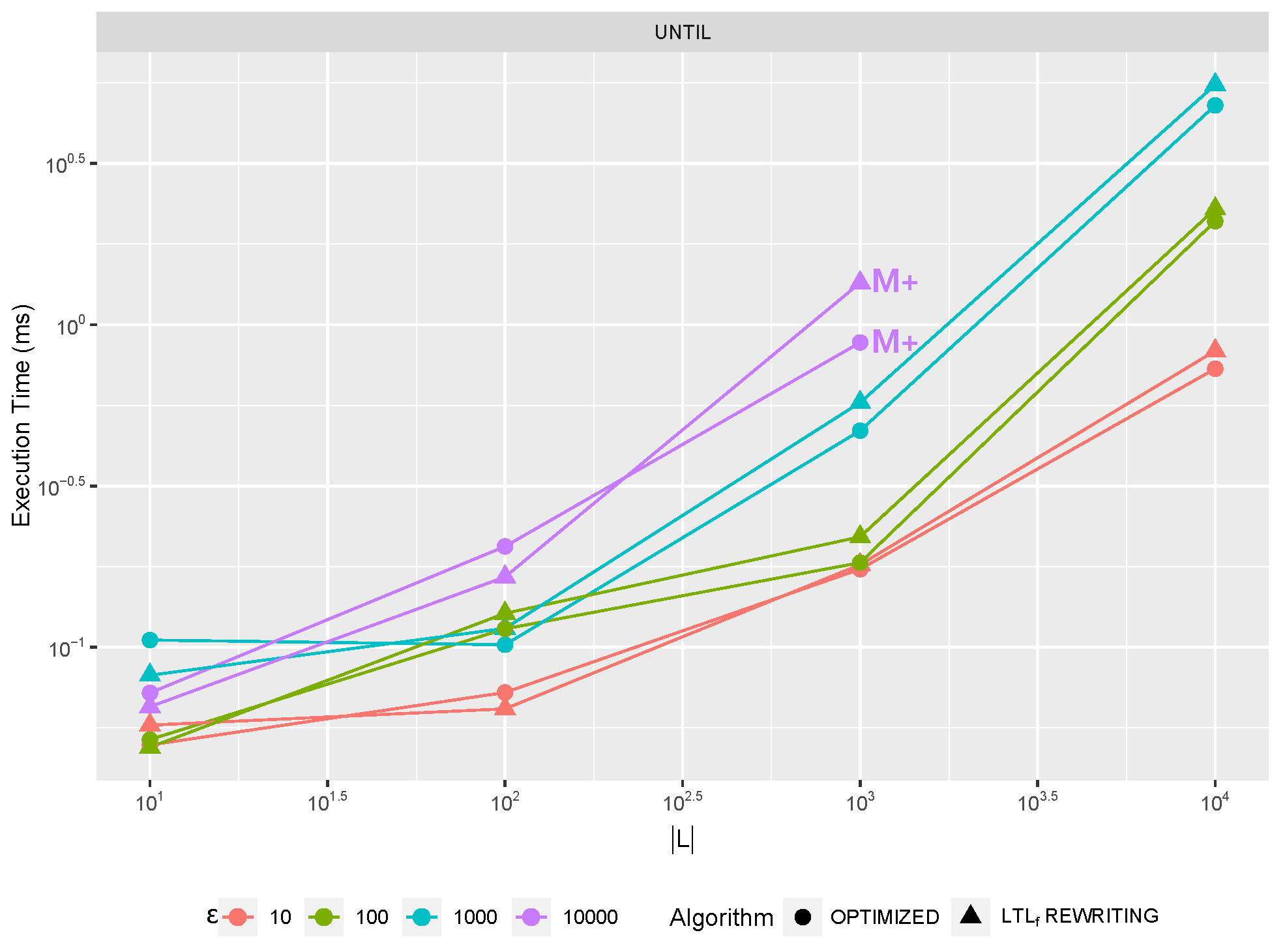
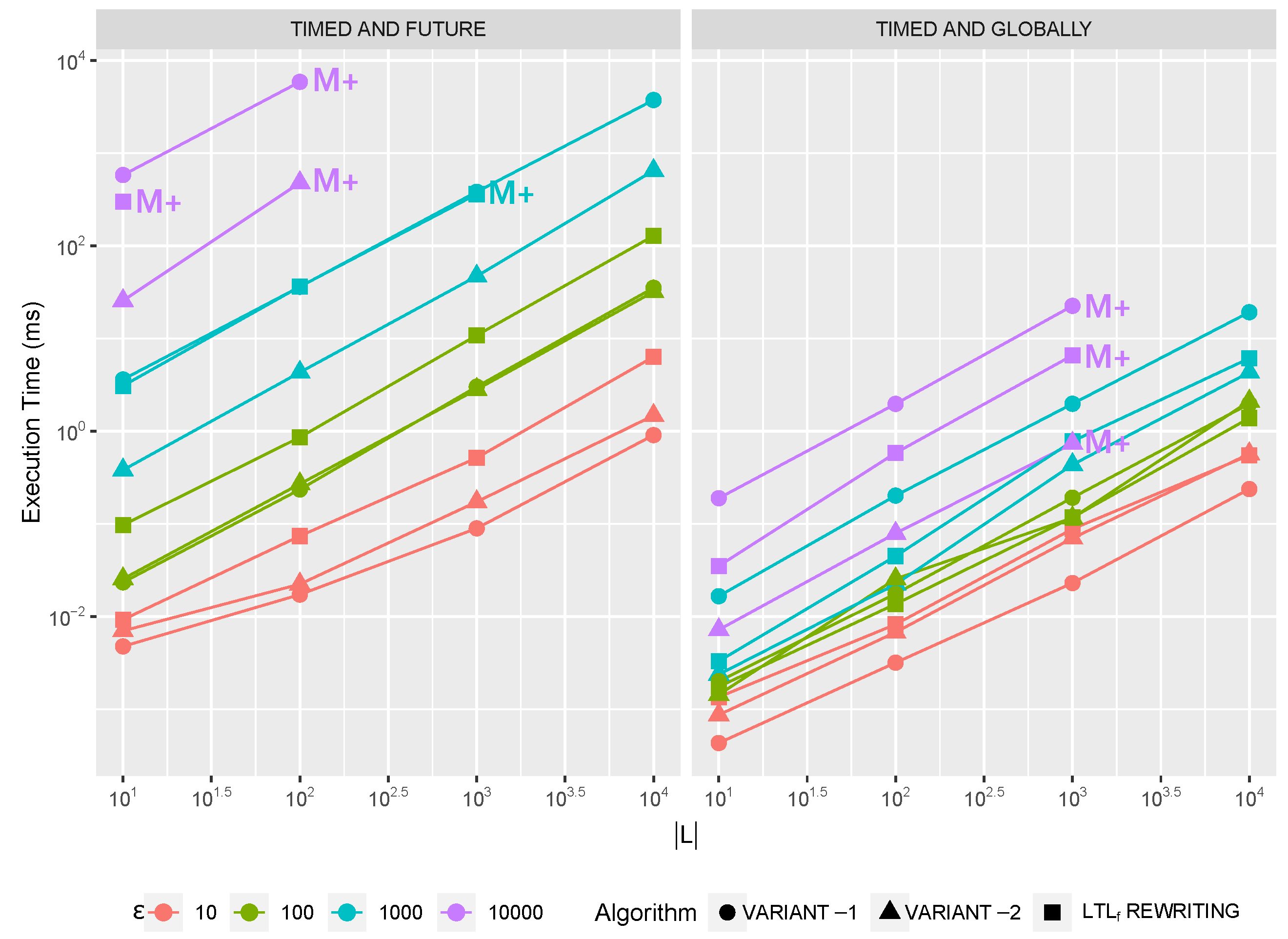
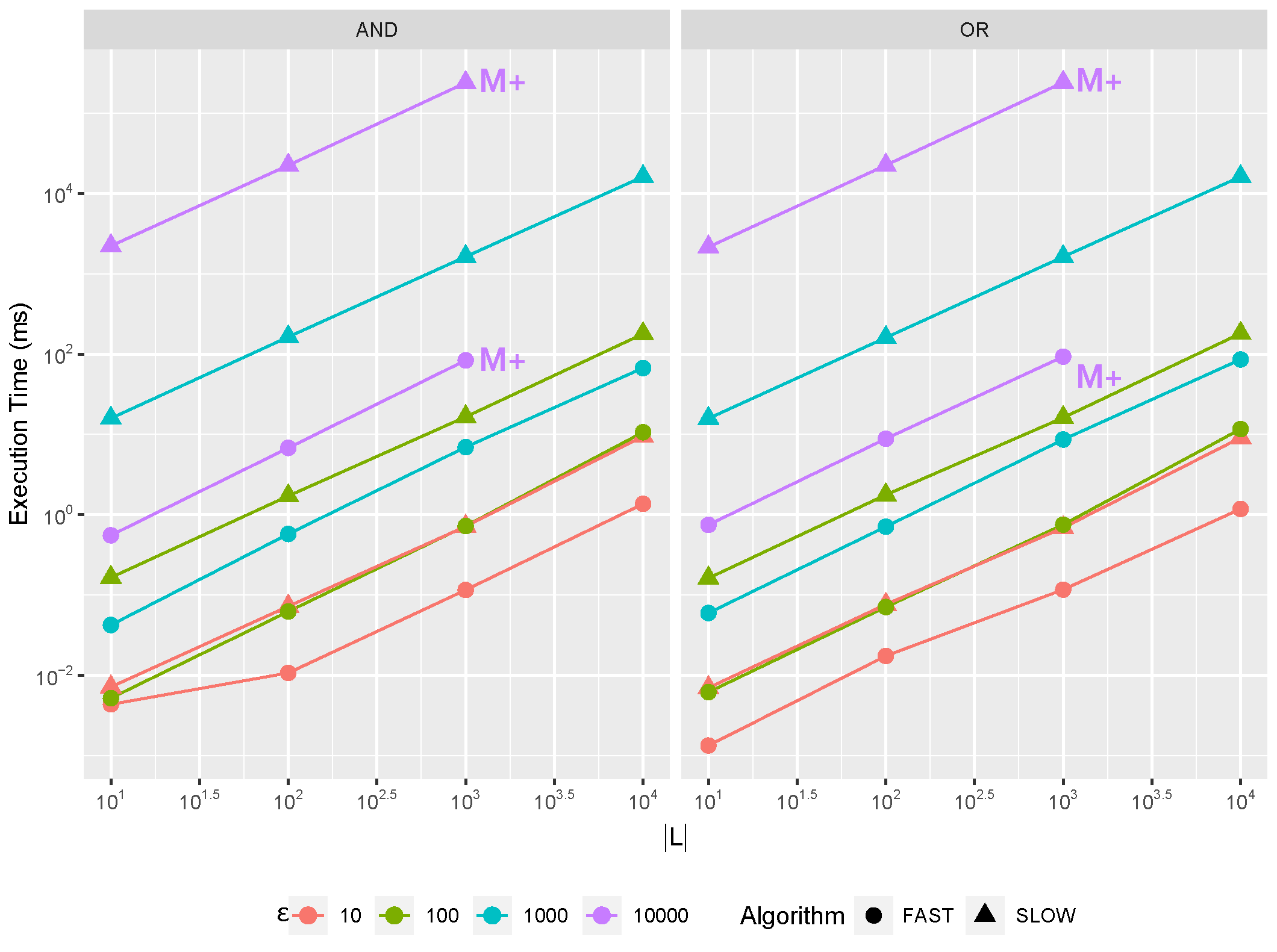
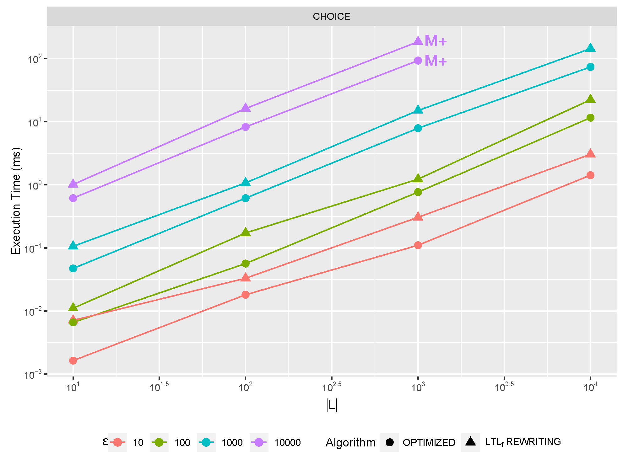
• Differently from our previous work, where we just hinted at the implementation of each operator with some high level, we now propose different possible algorithms for some xtLTL_f operators (Section 6), and we then discuss both theoretically (Supplement II.2) and empirically (Section 7.1) which might be preferred under different trace length $ϵ$ or log size $\left|\mathcal{L}\right|$ conditions. This leads to the definition of hybrid algorithms [8];
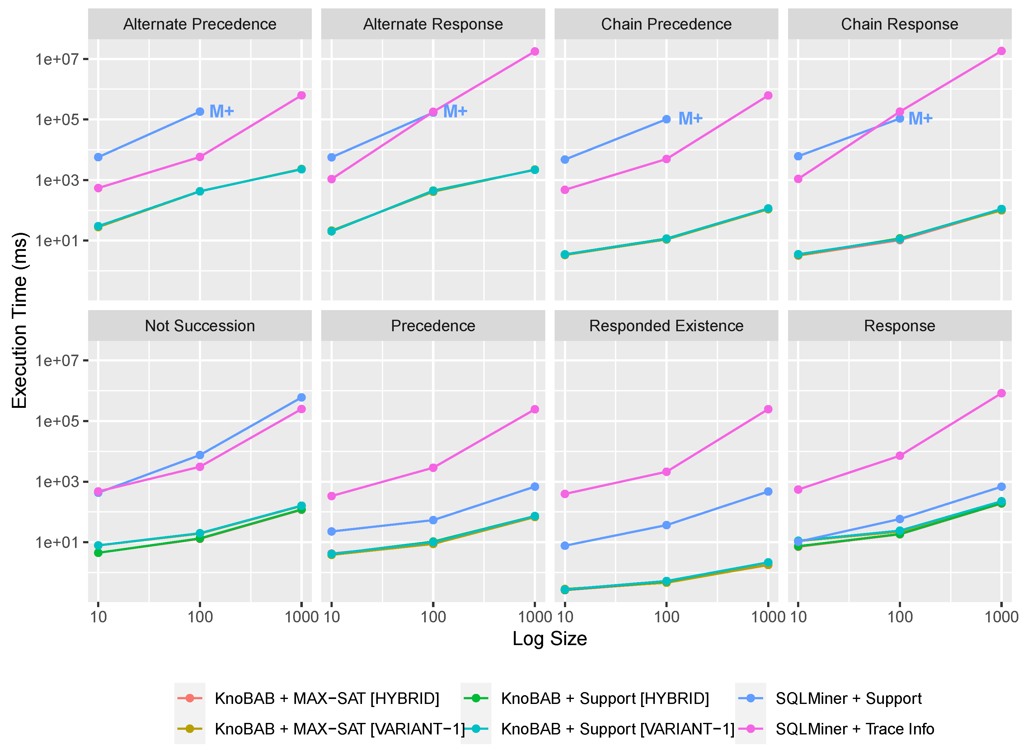
• Our benchmarks demonstrate that our implementation outperforms conformance checking techniques running on both relational databases (Section 7.2) and on tailored solutions (Section 7.5) when customary algorithms are chosen for implementing xtLTL_f  operators;
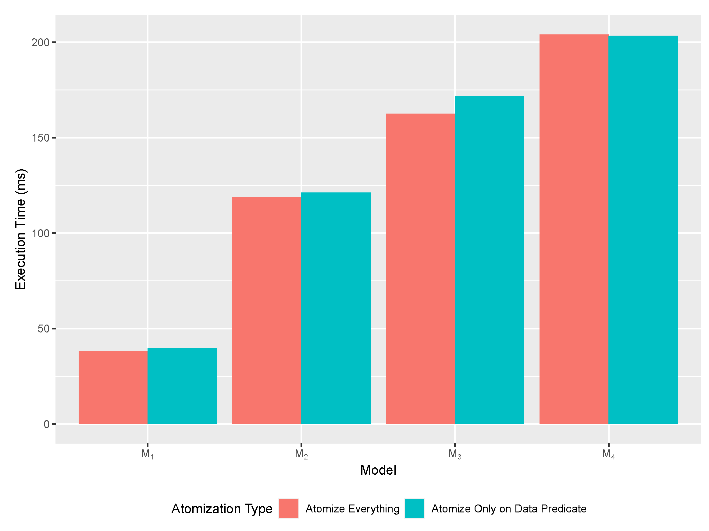
• Finally, this paper considerably extends the experimental section from our previous work. First, we show (Section 7.3) how the query plan’s execution might be parallelised, thus further improving with super-linear speed-up our previous running time results. Then, we also discuss (Section 7.4) how different data accessing strategies achievable through query rewriting might affect the query’s running time.

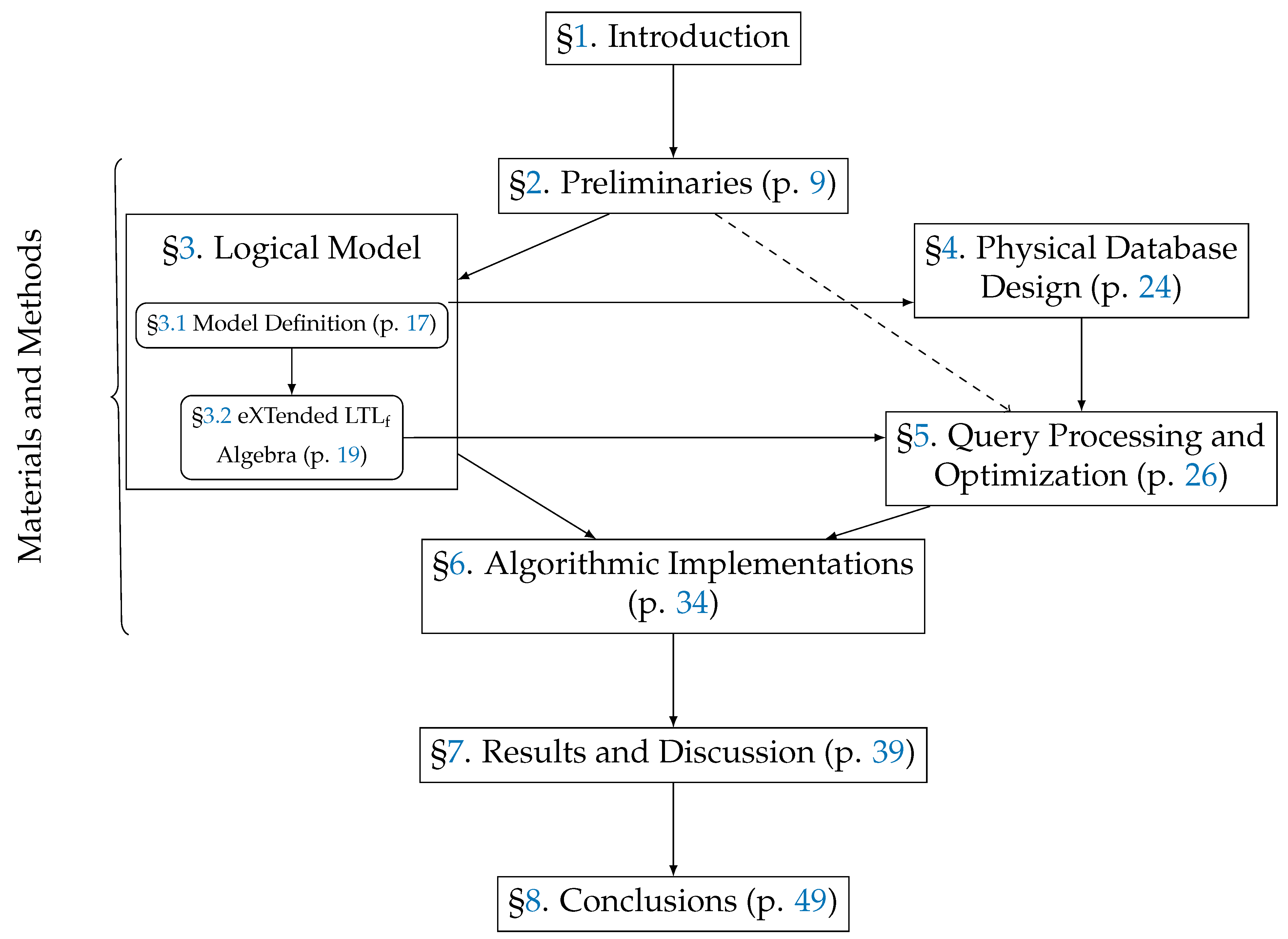
Figure 1 provides a graphical depiction of this paper’s table of contents, with the mutual dependencies between its sections. Appendices and Supplements start from p. 50.

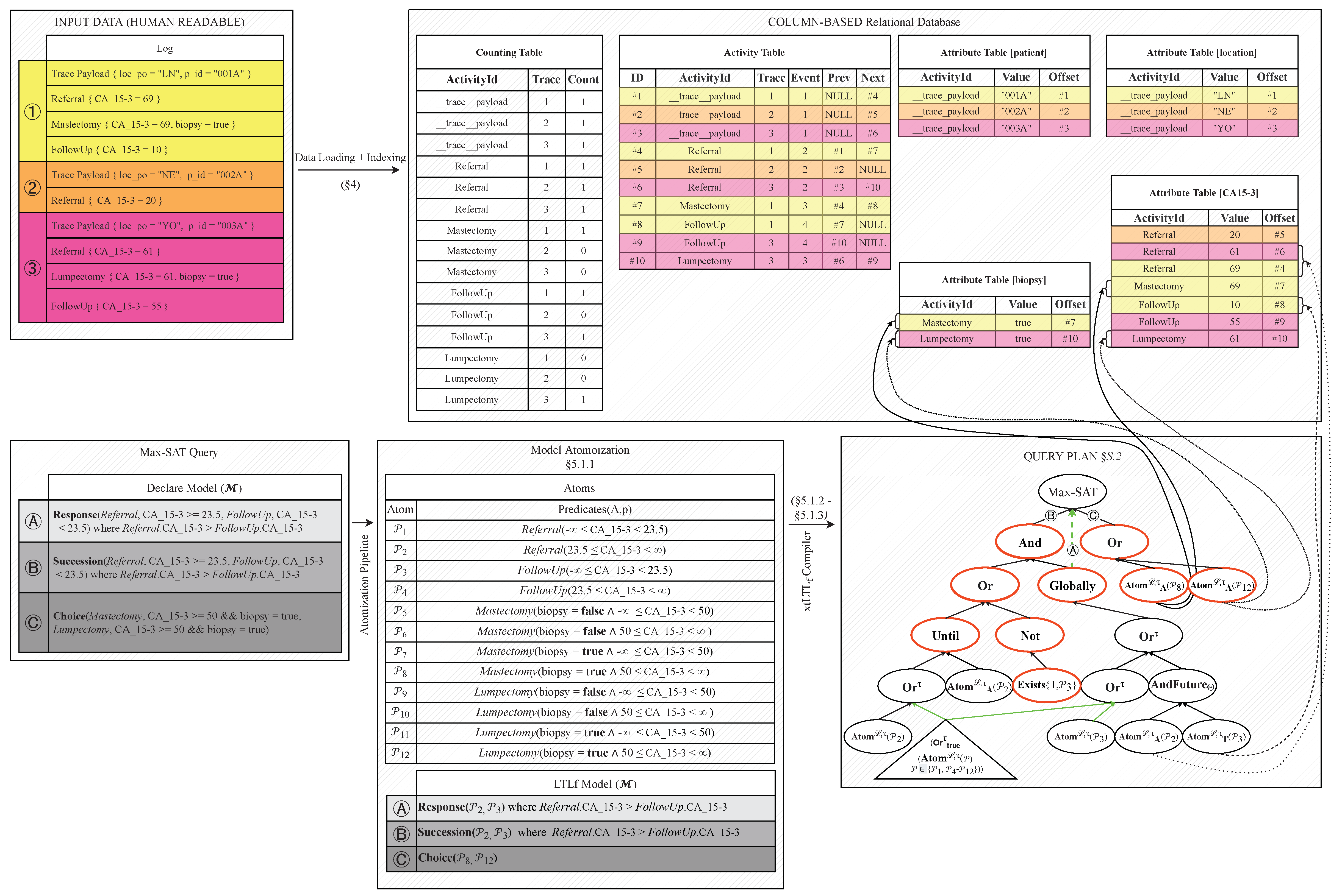
Figure 2 provides a bird-eye view of the overall KnoBAB architecture: in the upper half, we show how a log is loaded in our business process management system as a series of distinct tables providing some activity statistics (CountingTable) and full payload information (AttributeTable) in addition to reconstructing the unravelling of the events as described by their traces (ActivityTable). On the other hand, the lower half shows the main steps of the query engine transforming a declarative model into a DAG query plan accessing the previously-loaded relational tables. The most recent version of our system is on GitHub ( https://github.com/datagram-db/knobab as accessed the 5 March 2023). When not explicitly stated, all the links were last accessed the 5 March 2023.

1.1. Case Studies

The present section shows a broad-ranging set of real case studies requiring efficient conformance checking computations in LTL_f. This, therefore, motivates the need for our proposed approach in a practical sense.

1.1.1. Cyber Security

Intrusion detection for cyber security aims at auditing an environment for identifying potential flaws that can be remedied and fixed later. While anomaly-based approaches raise an alarm if the observed behaviour differs significantly from the expected one, signature-based approaches check whether attack patterns might be recognised from the environment. The latter are often used to mitigate the high false-alarm rates of the former [10]. Expected behaviour might be encoded as process models expressed in LTL_f, which, when violated, lead to the detection of an attack: such a language can be directly exploited to represent several different kinds of attacks, such as Denial Of Service, Buffer Overflows, and Password Guessing [10]. In his dissertation [11], Ray shows how malware can be detected by determining LTL_f formulae discriminating between system–calls patterns generated by malicious software from expected run-time behaviour. Recent developments [12,13] showed that it is possible to perform prediction (and therefore reasoning) on potentially infinite sequences by analysing a finite subsequence of the overall behaviour within a sliding window; Buschjäger et al. [12] predict future events not covered by the sliding window by correlating them to the patterns observed in such a window. By associating a positive label to each finite subsequence preceding or containing an attack, and a negative one otherwise, we can also extract temporal models detecting subsequences containing attacks [14]. This entails that real-time verification boils down, to some extent, to offline monitoring, as we guarantee that it is sufficient to analyse currently-observed behaviours to predict and detect an attack. The learned model, once validated, can be exploited in the aforementioned real-time verification systems [10].

Example 1.

The Cyber Kill Chain® framework (https://www.lockheedmartin.com/en-us/capabilities/cyber/cyber-kill-chain.html as accessed the 5 March 2023) allows the identification and prevention of intrusion activities on computer systems. This framework is based on a military tactic simply known as a kill chain (https://en.wikipedia.org/wiki/Kill_chain, 5 March 2023), which breaks down the attack into the following phases: target identification, marshalling and organizing forces towards the target, starting an attack, and target neutralisation. Lockheed Martin reformulated these steps to be transferred to the IT world and redirected the attack against a virtual target. These phases were reformulated as follows:

• Reconnaissance (rec): An attacker observes the situation from the outside in order to identify targets and tactics. As the attacker mainly collects information regarding the system’s vulnerabilities, this is the hardest part to detect.
• Weaponisation (weap): After gathering the information, the cybercriminal implements his strategy through a software artefact. This detection will have greater chances of success in the future after post-mortem analysis, when either a temporal model is mined over the collected attack data or the strategy is directly inferred from available artefacts (e.g., malaware).
• Payload or Delivery (del): The cybercriminal devises a way to infiltrate the host system that hides the previously produced artefact (e.g., a Trojan). This must sound as harmless as possible to fool the system.
• Exploitation (expl): The cybercriminal exploits the system’s vulnerabilities and infiltrates it through the previous “cover”. At this stage, the defensive system should raise the alarm if any kind of unusual behaviour is detected while increasing the security level.
• Installation (inst): The weapon escapes the payload and gets installed into the host computer system. At this point, any kind of suspected behaviour might be detected by malicious system calls.
• Command & Control (comm): The weapon establishes a communication with the cybercriminal for receiving orders from the attacker. The system should detect any kind of suspicious network communication and should attempt to break the communication channel.
• Action (act): The intruder starts the attack on the system. At this stage, the attack should be more evident, and the Industrial IoT Shields (iiot_sh), such as network devices protection, should be activated.

Figure 3a describes the actions (and therefore activity labels) of interest. Having defined the actions that should be monitored, records of activities can be stored as traces within a log. This is represented in Figure 3b, where we define three distinct attacks as distinct traces (${\sigma }_1,{\sigma }_2,{\sigma }_3$). Each trace contains the event information leading up to the completion of an attack attempt (which may be (un)successful). Data payload information is also considered, and here this is provided as the unique timestamp (ts) associated with each event. Trace payload information is not simulated here but is described and applied in Example 2.

A temporal model might describe a completely successful attack. The occurrence of the aforementioned phases can be described through a temporal declarative language Declare [7], where each constraint is an instantiated Declare clause (see

Table 1. Declare templates illustrated as exemplifying clauses. $A\wedge p$ ($B\wedge q$) represents the activation (target) condition, A (B) denotes the activity label, and p (q) is the data payload condition.

Type	Exemplifying Clause (${\mathit{c}}_{\mathit{l}}$)	Natural Language Specification for Traces	LTLf Semantics ($〚{\mathit{c}}_{\mathit{l}}〛$)
Simple	Init($A,p$)	The trace should start with an activation	$A\wedge p$
	Exists($A,p,n$)	Activations should occur at least n times	$\left\{\begin{array}{cc}\diamond (A\wedge p\wedge ◯(〚\mathtt{Exists}(A,p,n-1)〛\left)\right)\hfill & n>1\hfill \\ \diamond (A\wedge p)\hfill & n=1\hfill \end{array}\right.$
	Absence($A,p,n+1$)	Activations should occur at most n times	$\neg 〚\mathtt{Exists}$($A,p,n+1$)〛
	Precedence($A,p,B,q$)	Events preceding the activations should not satisfy the target	$\neg (B\wedge p)\mathcal{W}(A\wedge p)$
(Mutual) Correlation	ChainPrecedence($A,p,B,q$)	The activation is immediately preceded by the target.	$\square \left(◯\right(A\wedge p)\Rightarrow (B\wedge q\left)\right)$
	Choice($A,p,A^{\prime },p^{\prime }$)	At least one of the two activation conditions must appear.	$\diamond (A\wedge p)\vee \diamond (A^{\prime }\wedge p^{\prime })$
	Response($A,p,B,q$)	The activation is either followed by or simultaneous to the target.	$\square \left(\right(A\wedge p)\Rightarrow \diamond (B\wedge q\left)\right)$
	ChainResponse($A,p,B,q$)	The activation is immediately followed by the target.	$\square \left(\right(A\wedge p)\Rightarrow ◯(B\wedge q\left)\right)$
	RespExistence($A,p,B,q$)	The activation requires the existence of the target.	$\diamond (A\wedge p)\Rightarrow \diamond (B\wedge q)$
	ExclChoice($A,p,A^{\prime },p^{\prime }$)	Only one activation condition must happen.	$〚\mathtt{Choice}(\mathtt{A},p,{\mathtt{A}}^{\prime },p^{\prime })〛\wedge 〚\mathtt{NotCoExistence}(\mathtt{A},p,{\mathtt{A}}^{\prime },p^{\prime })〛$
	CoExistence($A,p,B,q$)	RespExistence, and vice versa.	$〚\mathtt{RespExistence}(\mathtt{A},p,\mathtt{B},q)〛\wedge 〚\mathtt{RespExistence}(\mathtt{B},q,\mathtt{A},p)〛$
	Succession($A,p,B,q$)	The target should only follow the activation.	$〚\mathtt{Precedence}(\mathtt{A},p,\mathtt{B},q)〛\wedge 〚\mathtt{Response}(\mathtt{A},p,\mathtt{B},q)〛$
	ChainSuccession($A,p,B,q$)	Activation immediately follows the target, and the target immediately preceeds the activation.	$\square \left(\right(A\wedge p)\iff ◯(B\wedge q\left)\right)$
	AltResponse($A,p,B,q$)	If an activation occurs, no other activations must happen until the target occurs.	$\square \left(\right(A\wedge p)\Rightarrow (\neg (A\wedge p)\mathcal{U}(B\wedge q)\left)\right)$
	AltPrecedence($A,p,B,q$)	Every activation must be preceded by an target, without any other activation in between	$〚\mathtt{Precedence}(\mathtt{A},p,\mathtt{B},q)〛\wedge \square \left(\right(A\wedge p)\Rightarrow ◯(\neg (A\wedge p)\mathcal{W}(B\wedge q))$
Not.	NotCoExistence($A,p,B,q$)	The activation nand the target happen.	$\neg (\diamond (A\wedge p)\wedge \diamond (B\wedge q\left)\right)$
	NotSuccession($A,p,B,q$)	The activation requires that no target condition should follow.	$\square \left(\right(A\wedge p)\Rightarrow \neg \diamond (B\wedge q\left)\right)$

). Our declarative language should be able to state the following requirements: Ⓐ all reconnaissance events should be followed by a weaponisation, Ⓑ there should be no IoT shields in place, and Ⓒ either command and control or action should occur.

On blockchains, each trace event represents a proper blockchain event, thus including function or event invocations issued by one or more smart contracts. In particular, smart contracts are sets of conditions specified in self-executing programs [15], which include protocols within which the parties will fulfil some promises [16]. Given that smart contracts can also be seen as postconditions activated upon the occurrence of specified pre-conditions [17], they are also exploited as security measures reducing malicious and accidental exceptions [15]. As per previous considerations, we can directly encode the smart contract premises in LTL_f, as well as represent the whole smart contract as a whole LTL_f formula under the assumption that the blockchain guarantees its execution [17]. Therefore, we can perform post-mortem analysis checking whether a given run-time abides by the rules imposed by the system.

1.1.2. Industry 4.0

Smart factories enable the collection and analysis of data through advanced sensors and embedded software for better decision-making. These enable monitoring each phase of the entire production process in both real-time and domain-specific applications where the safety of both autonomous cyber-physical systems as well as human workers is at stake [18]. This is of the uttermost importance, as both humans and machines cooperate in the same environment where a minimal violation of safety requirements might damage the overall production process, thus reflecting in maintenance costs. This calls for logical-based formal methods providing correctness guarantees [19]. Run-time verification [19] and prediction [13] have started gaining momentum against customary static analysis tools: in fact, real complex systems such as factories are often hard to predict and analyse before execution. As run-time verification can be deployed as a permanent testing condition on the environment, Mao et al. [19] show that this approach is complete, thus reducing the complicated model-checking problem into a simpler conformance checking one. Programmable Logic Controllers (PLC) are at the heart of this mechanism, where controllers can make decisions over previously-observed events. PLC work is similar to smart contracts in the previous scenario: at each “scan cycle”, the controllers perceive through sensors the status change of the environment (e.g., variations of temperature and pressure). This information is then fed to the internal logic, which, on the other hand, might decide to intervene directly in the environment by sending signals to some actuators (e.g., controlling the pressure and temperature on the system). Due to the similarity of PLC to smart contracts, these might also exploit LTL_f for determining security requirements: when a safety condition is violated, the PLC might activate an alarm while ensuring that the system works within safe operation ranges [19]. Please observe that ptLTL, also defined in [19], is a version of LTL allowing reasoning on past events so as to avoid semi-decidable computations for traces of infinite length, might be still represented through an equivalent LTL_f formula evaluated over a finite sliding window [13] bounded by the first and the latest event. Please observe that the difference between LTL and LTL_f  is that only the latter considers traces of finite length.

In some other industrial scenarios, we might be interested in detecting unexpected variations in time series reflecting the fluctuation of some perceived variables (e.g., variations in temperature and pressure). The latest developments [13] showed that (industrial) time series could also be represented as traces: we might assign to each event an activity label $\varpi$ if the current event has a data payload whose values upper bound the ones from immediately preceding event’s payload, and $\neg \varpi$ otherwise. Consequently, we can encode disparate data variation patterns in LTL_f reflecting different types of data volatility or steep increases/decreases [13]. This shows how LTL_f can also represent anomaly-based problems by reducing them to the identification of anomaly patterns [20].

1.1.3. Healthcare

A medical process describes clinical-related procedures as well as organisational management ones (e.g., registration, admission, and discharge) [21]. The renowned openEHR (https://www.openehr.org/ accessed the 5 March 2023) standard distinguishes the former in four main archetypes: an observation, recording patients’ clinical symptoms (e.g., body temperature, blood pressure); an evaluation, providing preliminary diagnosis and assessing the patient’s health based on the former results; and an instruction, the execution of the treatment plan proposed by a physician (e.g., prescribing, examining, and testing). An action describes the way to intervene or treat medical patients according to the treatment plan (e.g., drug administration, blood matching). Once encoded as such, each process representing an instantiation of a medical process, i.e., a patient’s clinical course, can be then collected and represented in a log. As such, each action is going to be represented as a distinct activity label of a given event [22] that might contain relevant payload information recording the outcome of the clinical procedures, as well as demographical information related to the patient [21] for future socio-clinical analyses [23].

Declarative temporal languages such as Declare can then be exploited to provide a descriptive approach specifying temporal constraints among activities without strictly enforcing their order of completion, thus restricting the order of application of a specific set of activities [21]. As these models come with temporal semantics expressed in LTL_f, these are, for all intents and purposes, process models. As such, these might be applied to detect discrepancies between clinical guidelines, expressed by the aforementioned model, and the actual process executions collected in a log. This is of the utmost concern as often deviations represent errors compromising the patient recovery [22], which, if efficiently and identified in advance, lead to an increased patient satisfaction as well a reduction of healthcare costs (e.g., due to mismanagement) [21].

Example 2.

To minimise costs and unrequired procedures, only ill patients should receive treatment. Thus, sufferers not receiving treatment (false negatives) and non-sufferers receiving treatment (false positives) need to be minimised. Figure 2 proposes a simplified scenario where we consider two event payload keys: CA 15-3 (cancer antigen concentration in a patient’s blood) and biopsy (biopsies should be taken before any procedure is acted upon). Our model targets only breast cancer patients with successful therapies that describe a medical protocol and the desired patients’ health condition at each step. Ⓒ states that two possible surgical operations for breast tumours are mastectomy or lumpectomy if the biopsy is positive and the CA-13.5 is way above ($\ge 50$) the guard level, being 23.5 units per mL, and Ⓐ–Ⓑ any successful treatment should decrease the CA-13.5 levels, which should be below the guard level; such correlation data condition is expressed via a Θ condition (introduced by a $\mathsf{where}$). A twinned negative model (not in Figure) might better discriminate healthy patients from patients where the therapy was unsuccessful. Novel situations can be represented as a log. For example, in Figure 2, we have three patients: ➀ a cancer patient with a successful mastectomy, ➁ a healthy patient, and ➂ an unsuccessful lumpectomy, thus suggesting that the patient might still have some cancerous cells. Given the aforementioned model, patient ➀ will satisfy the model as the surgical operation was successful, ➁ will not satisfy the model because neither a mastectomy nor a lumpectomy was required ($\mathcal{M}$ is only fulfilled for successful procedures), and ➂ will not satisfy the target condition, even though the correlation condition was met. Our model of interest should only return ➀ as an outcome of the conformance checking process.

2. Preliminaries

eXtensible Event Stream (XES). This paper relies on temporal data represented as a temporally ordered sequence of events (trace or streams), where events are associated with at most one action described by a single activity label [24]. In this paper, we formally characterize payloads as part of both events and traces while, in our previous work, we only considered payloads from events [25].

Given an arbitrarily ordered set of keys K and a set of values V, a tuple [26] is a finite function $p:K\to V$ (also $p\in V^K$), where each key is either associated with a value in V or is undefined. After denoting ⊥ as a null element missing from the set of values ($\perp \notin V$), we can express that $\kappa$ is not associated with a value in p as $p\left(\kappa \right)=\perp$, thus $\kappa \notin dom\left(p\right)$. An empty tuple $\epsilon$ has an empty domain.

(Data) payloads are tuples, where values can represent either categorical data or numerical data. An event ${\sigma }_j^i$ is a pair $〈\mathtt{a},p〉\in \Sigma \times V^K$, where $\Sigma$ is a finite set of activity labels, and p is a finite function describing the data payload. A trace ${\sigma }^i$ is an ordered sequence of distinct events ${\sigma }_1^i,\cdots ,{\sigma }_n^i$, which is distinguished from the other traces by a case id i; n represents the trace’s length ($n=|{\sigma }^i|$). If a payload is also associated with the whole trace, this can be easily mimicked by adding an extra initial event containing such a payload with an associated label of __trace_payload. A log$\mathcal{L}$ is a finite set of traces $\left\{{\sigma }^1,\cdots ,{\sigma }^m\right\}$. In this paper, we further restrict our interest to the traces containing at least one event, as empty traces are meaningless as they are not describing any temporal behaviour of interest. Finally, we denote as $\beta :\Sigma \leftrightarrow \left\{1,\cdots ,|\Sigma |\right\}$ the bijection mapping each activity label occurring in the log to an unique id.

Example 3.

The log $\mathcal{L}$ in Figure 2 comprises three distinct traces $\mathcal{L}=\left\{{\sigma }^1,{\sigma }^2,{\sigma }^3\right\}$. In particular, the second trace comprises two events ${\sigma }^2={\sigma }_1^2{\sigma }_2^2$, where the first event represents the trace payload, and therefore ${\sigma }_1^2=\langle \_\_\mathsf{trace}\_\mathsf{payload},p\rangle$ having $p(\mathit{loc}\_\mathit{po})=NE$ and $p(\mathit{p}\_\mathit{id})=002A$. The other event is ${\sigma }_2^2=\langle \mathsf{Referral},\tilde{p}\rangle$, where payload $\tilde{p}$ is only associated with the CA-13.5 levels as $\tilde{p}(\mathit{CA}-\mathit{13}.\mathit{5})=20$. Similar considerations can be carried out for the other log traces.

Linear Temporal Logic over finite traces (LTL_f). LTL_f is a well-established extension of modal logic considering the possible worlds as finite traces, where each event represents a single relevant instant of time. The time is thereby linear, discrete, and future-oriented. This entails that that the events represented in each trace are totally ordered and, as LTL_f quantifies only on events reported in the trace, all the events of interest are fully observable. The syntax of an well-formed LTL_f formula $\phi$ is defined as follows:

$$\phi ::=\mathtt{a}|\neg \phi |\phi \vee {\phi }^{\prime }|\phi \wedge {\phi }^{\prime }\left|{\displaystyle ◯}\phi \right|\square \phi |\diamond \phi |\phi \mathcal{U}{\phi }^{\prime }$$

(1)

where $\mathtt{a}\in \Sigma$. Its semantics is usually defined in terms of First Order Logic [27] for a given trace ${\sigma }^i$ at a current time j (e.g., for event ${\sigma }_j^i$) as follows:

• An event satisfies the activity label $\mathtt{a}$ iff. its activity labels is $\mathtt{a}$: ${\sigma }_j^i\vDash \mathtt{a}\iff {\sigma }_j^i=\langle \mathtt{a},p\rangle$;
• An event satisfies the negated formula iff. the same event does not satisfy the non-negated formula: ${\sigma }_j^i\vDash \neg \phi \iff {\sigma }_j^i⊭\phi$;
• An event satisfies the disjunction of LTL_f sub-formulæ iff. the event satisfies one of the two sub-formulæ: ${\sigma }_j^i\vDash \phi \vee {\phi }^{\prime }\iff {\sigma }_j^i\vDash \phi \vee {\sigma }_j^i\vDash {\phi }^{\prime }$;
• An event satisfies the conjunction of LTL_f formulæ iff. the event satisfies all of the sub-formulæ: ${\sigma }_j^i\vDash \phi \wedge {\phi }^{\prime }\iff {\sigma }_j^i\vDash \phi \wedge {\sigma }_j^i\vDash {\phi }^{\prime }$;
• An event satisfies a formula at the next step iff. the formula is satisfied in the incoming event if present: ${\sigma }_j^i\vDash ◯\phi \iff i<\left|{\sigma }_j\right|\wedge {\sigma }_{j+1}^i\vDash \phi$;
• An event globally satisfies a formula iff. the formula is satisfied in all the following events, including the current one: ${\sigma }_j^i\vDash \square \phi \iff \forall j\le x\le \left|{\sigma }^i\right|.{\sigma }_x^i\vDash \phi$;
• An event eventually satisfies a formula iff. the formula is satisfied in either the present or in any future event: ${\sigma }_j^i\vDash \diamond \phi \iff \exists j\le x\le \left|{\sigma }^i\right|.{\sigma }_x^i\vDash \phi$;
• An event satisfies $\phi$ until ${\phi }^{\prime }$ holds iff. $\phi$ holds at least until ${\phi }^{\prime }$ becomes true, which must hold at the current or a future position: ${\sigma }_j^i\vDash \phi \mathcal{U}{\phi }^{\prime }\iff \exists j\le y\le \left|{\sigma }^i\right|.{\sigma }_y^i\vDash {\phi }^{\prime }\wedge \left(\forall x\le z<y.{\sigma }_z^i\vDash \phi \right)$

Other operators can be seen as syntactic sugar: Weak-Until is denoted as $\phi \mathcal{W}{\phi }^{\prime }:=\phi \mathcal{U}{\phi }^{\prime }\vee \square \phi$, while the implication can be rewritten as $\phi \Rightarrow {\phi }^{\prime }:=(\neg \phi )\vee (\phi \wedge {\phi }^{\prime })$. Generally, binary operators bridge activation and target conditions appearing in two distinct sub-formulæ. The semantics associated with activity labels, consistently with the literature on business process execution traces [25], assumes that, in each point of the sequence, one and only one element from $\Sigma$ holds. We state that a trace ${\sigma }^i$ is conformant to an LTL_f formula iff. it satisfies it starting from the first event: ${\sigma }^i\vDash \phi \iff {\sigma }_1^i\vDash \phi$, and is deviant otherwise [25]. The Declare language described in the next paragraph provides an application for such logic. As relational algebra describes the semantics for SQL [28,29], LTL_f is extensively applied [30] as a semantics for formally expressing temporal and human-readable declarative constraints such as Declare.

At the time of the writing, different authors proposed several extensions for representing data conditions in LTL_f. The simplest extensions are compound conditions $\mathtt{a}\wedge q$, which are the conjunction of data predicate $q\in \mathbf{Prop}$ to the activity label a [25]. Nevertheless, this straightforward solution is not able to express correlation conditions in the data which might be relevant in business scenarios [31], as representing correlations as single atoms requires decomposing the former into disjunctions of formulae [32]. Despite prior attempts to define a temporal logic expressing correlation conditions, no explicit formal semantics on how this can be evaluated was provided [6]. This poses a problem to the current practitioner, as this hinders the process of both checking formally the equivalence among two languages expressing correlation conditions, as well as providing a correct implementation of such an operator. We, on the other hand, propose a relational representation of xtLTL_f, where the semantics of all of the operators, thus including the ones requiring correlation conditions, is clearly laid out and implemented.

Declare. Temporal declarative languages pinpoint highly variable scenarios, where state machines provide complicated graph models that can be hardly understandable by the common business stake-holder [33]. Among all possible temporal declarative languages, we constrain our interest to Declare, originally proposed in [7]. Every single temporal pattern is expressed through templates (i.e., an abstract parameterised property: Table 1 column 2), which are parametrised over activation, target, or correlation conditions. Template names induce the semantic representation in LTL_f $〚c_l〛$ of each model clause $c_l$. Therefore, a trace ${\sigma }^i$ is conformant to a Declare clause iff. it satisfies its associated semantic representation in LTL_f (${\sigma }^i\vDash c_l\iff {\sigma }^i\vDash 〚c_l〛$). At this stage, activation (and target) conditions are predicates $A\wedge p$ (and $B\wedge q$) in such a clause asserting required properties for the events’ activity label ($A$ and $B$) and payload (p and q). An event in a given trace activates (or targets) a given clause if they satisfy the activation (or target) condition. Please observe that neither activation nor target conditions postulate the temporal (co)occurrence between activating or targeting events, as this is duty is transferred to the specific LTL_f semantics of the clause. A trace vacuously satisfies a clause if the trace satisfies the clause despite no event in the trace satisfied the activation condition. After this, we state that a trace non-vacuously satisfies the declarative clause if the trace satisfies the clause and one of the following conditions is satisfied:

• The clause provides no target condition and it exists at least one activating event;
• The clause provides a target condition but no binary (payload) predicate $\Theta$, and the declarative clause establishes a temporal correlation between (at least one) activating event and (at least one) targeting one;
• The clause provides both a target condition and a binary predicate $\Theta$, while the activating and targeting events satisfying the temporal correlation as in the previous case also satisfy a binary $\Theta$ predicate over their payloads; in this situation, we state that the activating and targeting event match as they jointly satisfy the correlation condition $\Theta$.

Finally, the presence of activating events is a necessary condition for non-vacuous satisfiability.

We can then categorize each Declare template from [30] through these conditions and the ability to express correlations between two temporally distant events happening in one trace: simple templates (Table 1, rows 1–3) only involving activation conditions; (mutual) correlation templates (rows from 4 to 15), which describe a dependency between activation and target conditions, thus including correlations between the two; and negative relation templates (last 2 rows), which describe a negative dependency between two events in correlation. Despite these templates possibly appearing quite similar, they generate completely different finite state machines, thus suggesting that these conditions are not interchangeable (http://ltlf2dfa.diag.uniroma1.it/, 5 March 2023). 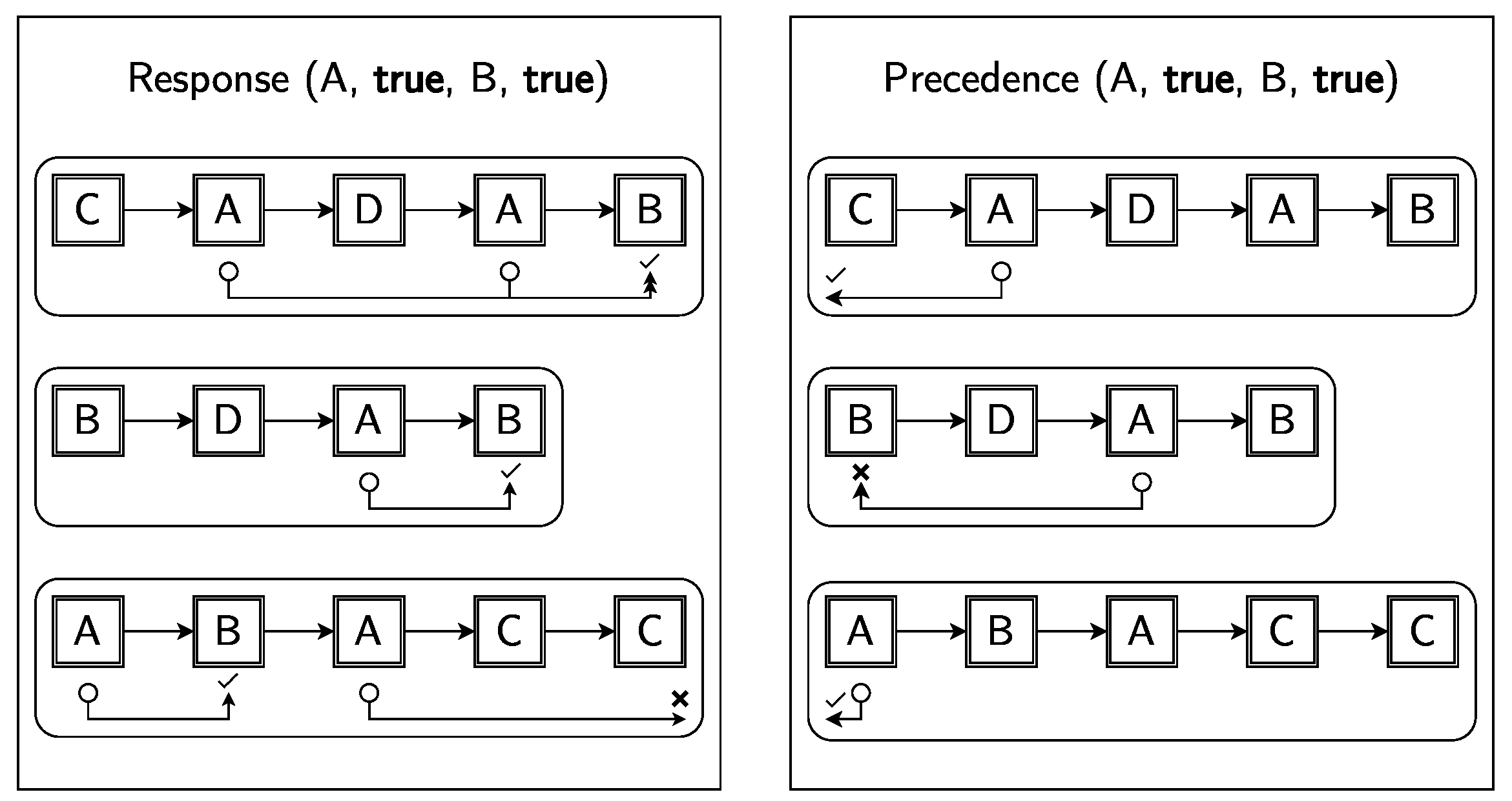Figure 4 exemplifies the behavioural difference between two clauses differing only on the template of choice.

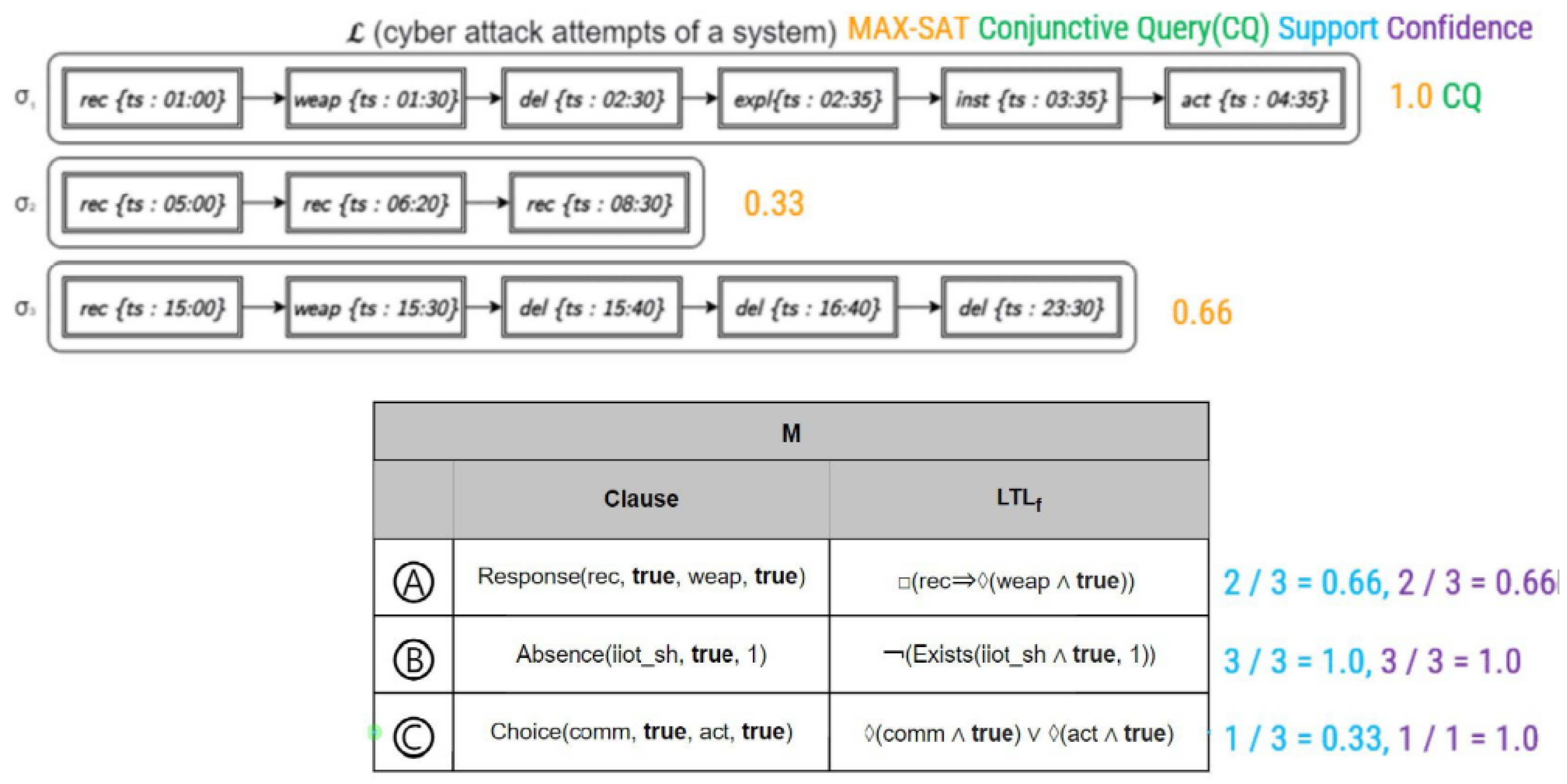
A Declare Model is composed of a set of clauses $\mathcal{M}={\left\{c_l\right\}}_{l\le n,n\in \mathbb{N}}$ which have to be contemporarily satisfied in order to be true. A trace ${\sigma }^i$ is conformant to a model $\mathcal{M}$ iff. such a trace satisfies each LTL_f formula $〚c_l〛$ associated with the model clause $c_l\in \mathcal{M}$. Consequently, a Declare model can be represented as a finitary conjunction of the LTL_f representation of each of its clauses, $〚\mathcal{M}〛:={\bigwedge }_{c_l\in \mathcal{M}}〚c_l〛$: for this, the Maximum-SATisfiability problem (Max-SAT) for each trace counts the ratio between the satisfied clauses over the whole model size. This consideration can be extended later on to also data predicates through predicate atomisation [25], as discussed in the next paragraph.

Relational Models and Algebras. The relational model was firstly introduced by Codd [34] to compactly operate over tuples grouped into tables. Such tables are represented as mathematical n-ary relations ℜ that can be handled through a relational algebra. Upon the effective implementation of the first Relational Database Management Systems (RDBMS), such algebra expressed the semantics of the well-known declarative query language, SQL. The rewriting of SQL in algebraic terms allowed the efficient execution of the declarative queries through abstract syntax tree manipulations [28]. Our proposed xtLTL_f (Section 3.2) takes inspiration from this historical precedent, in order to run conformance checking and temporal model mining queries over an relational representation of the log via relational tables (Section 3.1).

More recently, column-oriented DBMS such as MonetDB [35] proposed a new way to store data tables: instead of representing these per row, these were stored by column. There are several advantages to this approach, including better access to data when querying only a subset of columns (by eliminating the need to read columns that are not relevant) as well as discarding null-valued cells. This is achieved by representing each relation $\Re (\mathtt{id},A_1,\cdots ,A_n)$ in the database schema as distinct binary relations ${\Re }_{A_i}(\mathtt{id},A_i)$ for each attribute $A_i$ in ℜ. As this decomposition guarantees that the full-outer natural join ${\bowtie }_{1\le i\le n}{\Re }_{A_i}$ over the decomposed tables is equivalent to the initial relation $\Re$, we can avoid representing NULL values in each single binary relation, thus limiting our space allocation to the values effectively present in the data. We therefore took inspiration from this intuition for representing the payload information, thus storing one single table per payload attribute. To further optimise the query engine, it is also possible to boost the query performance by guaranteeing that the results always have a fixed schema, mainly listing the record ids satisfying the query conditions [36]. As we will see while introducing our temporal operators (Section 3.2), we will also guarantee that each operator returns the output in the same schema, thus guaranteeing time and memory optimality.

Finally, the nested relational model [37] extends the relational model by relaxing its first normal form (1NF), thus allowing table cells to contain tables and relations as values. Relaxing this 1NF allows for storing data in a hierarchical way in order to access an entire sub-tree with a single read operation. We will leverage this representation for our intermediate result representation, in order to associate multiple activation, target, or correlation conditions to one single event, thus including any relevant future event occurring after it.

Common Subquery Problem. Query caching mechanisms [38] are customary solutions for improving query runtime by holding partially-computed results in temporary tables referred to as materialised views, under the assumption that the queries sharing common data are pipelined [39]. Recently, Kechar et al. [9] proposed a novel approach that can also be run when queries are run contemporarily: it is sufficient to find the shared subqueries before actually running them so that, when they are run, their result is stored into materialised views thus guaranteeing that these are computed at most once.

Example 4.

Figure 2 shows how this idea might be transferred to our use case scenario requiring running multiple declarative clauses: Response is both a subquery of Succession as well as a distinct declarative clause of interest. Green arrows indicate operators’ output shared among operators expressed in our proposed xt LTL_f extension of xt LTL_f. Please also observe that operators with the same name and arguments but marked either with activation, target, or no specification are considered different as they provide different results, and therefore are not merged together. This includes distinctions between timed and untimed operators, which will be discussed in greater detail in Section 3.2.

To further minimize tables’ access times, it is possible to take this reasoning to its extreme by minimising the data access per data predicate in order to avoid accessing the same table multiple times. In order to do so, we need to partition the data space according to the queries at our disposal as in our previous work [25]. This process can be eased if we assume that each payload condition p and $p^{\prime }$ for the declarative clauses within a model $\mathcal{M}$ is represented in Disjunctive Normal Form (DNF) [40]: in this scenario, data predicates q are in DNF if they are a disjunction of one or more conjunctions of one or more data intervals referring to just one payload key.

Example 5.

The model illustrated in Figure 3a and discussed in former Example 1 comes with data conditions associated with neither activation nor target conditions. Therefore, no atomisation process is performed. Thus, each event in a log might just be distinguished by its activity label [25].

Given an LTL_f expression $\phi$ containing compound conditions, we denote ${\mathcal{D}}_{\phi }$ as the set of distinct compound conditions in $\phi$. We refer to the items in ${\mathcal{D}}_{\phi }$ as atoms iff. for each pair of distinct compound conditions in it, they never jointly satisfy any possible payload p (More formally, $\forall p.\forall \mathtt{a}\in \Sigma .\forall \mathtt{a}\wedge q,\mathtt{a}\wedge q^{\prime }\in {\mathcal{D}}_{\phi }.(q\ne q^{\prime })\Rightarrow (q\left(p\right)\Rightarrow \neg q^{\prime }\left(p\right))$). Ref. [25] shows a procedure showing how any formula $\phi$ can be rewritten into an equivalent one ${\phi }^{\prime }$ by ensuring that ${\mathcal{D}}_{{\phi }^{\prime }}$ contains atoms. This can be achieved by constructing ${\mathcal{D}}_{{\phi }^{\prime }}$ first from $\phi$ (Algorithm 1), and then converting each compound conditions in $\phi$ as disjunctions of atoms in ${\mathcal{D}}_{{\phi }^{\prime }}$, thus obtaining ${\phi }^{\prime }$.

Algorithm 1 Atomisation: ${\mathcal{D}}_{\phi }$-encoding pipeline.

1: global $\mu \leftarrow \left\{\right\}$; $ad\leftarrow \left\{\right\}$; $ak\leftarrow \left\{\right\}$       2: procedure CollectIntervals($\mathtt{a}$, DNF)$$ ▹ DNF$:={\bigvee }_{1\le i\le n}{\bigwedge }_{1\le k\le m\left(i\right)}{\mathit{low}}_{i,k}\le k_{i,k}\le {\mathit{up}}_{i,k}$   3:     for all  $\mathit{conj}\in DNF$ and $\mathit{low}\le k\le \mathit{up}\in \mathit{conj}$ do   4:         $\mu (\mathtt{a},k).\mathtt{put}\left(\right[\mathit{low},\mathit{up}\left]\right)$   5:     end for       6: procedure CollectIntervals($\mathcal{M}$)$$ ▹$\mathcal{M}:={\bigwedge }_{1\le i\le \left|\mathcal{M}\right|}{\mathtt{clause}}_i(\mathtt{A},p,\mathtt{B},p^{\prime })$   7:     for all ${\mathtt{clause}}_i(\mathtt{A},p,\mathtt{B},p^{\prime })\in \mathcal{M}$ do   8:         if $p\ne \mathbf{True}$ then CollectIntervals($\mathtt{A},p$)   9:         if $p^{\prime }\ne \mathbf{True}$ then CollectIntervals($\mathtt{B},p^{\prime }$) 10:     end for     11: procedure ${\mathcal{D}}_{\phi }$-encoding( ) 12:     for all $\mathtt{a}\in \Sigma$ do 13:         for all $k\in K$ do 14:            $\mu (\mathtt{a},k)\leftarrow$SegmentTree($\mu (\mathtt{a},k)$) 15:         end for 16:         for all $\mathit{partition}{\in }_{k\in K}\mu (\mathtt{a},k).\mathtt{elementaryIntervals}\left(\right)$ do$$ ▹$\mathit{partition}:={\left({\mathit{low}}_k\le k\le {\mathit{up}}_k\right)}_{k\in K}$ 17:            $p_i\leftarrow$new atom() 18:            $p_i:=\mathtt{a}\wedge \mathit{partition}$ 19:            $ak\left(\mathtt{a}\right).\mathtt{put}\left(p_i\right)$ 20:            for all ${\mathit{low}}_k\le k\le {\mathit{up}}_k\in \mathit{partition}$ do 21:                $ad(\mathtt{a},{\mathit{low}}_k\le k\le {\mathit{up}}_k).\mathtt{put}\left(p_i\right)$ 22:            end for 23:         end for 24:         if $ak\left({a}\right)=\varnothing$ then 25:            $ak\left(\mathtt{a}\right)\leftarrow \left\{\mathtt{a}\right\}$ 26:         end if 27:     end for

We collect all the conjunctions referring to the same payload key into a map μ(a,κ) (Line 4). After doing so, we can construct a Segment Tree [41] from the intervals in μ(a,κ), thus identifying the elementary intervals partitioning the collected intervals (Line 14). These elementary intervals also partition the payload data space associated with events for each activity label a. This can be achieved by combining each elementary interval in each dimension $\kappa$ for a (Line 16) and then associating it with a new atom representing such a partition (Line 18) that is then guaranteed to be an atom by construction. This entails that each interval ${\mathit{low}}_{\kappa }\le \kappa \le {\mathit{up}}_{\kappa }$ will be characterised by the disjunction of all of the atoms $p_i$ comprising such interval (Line 21). Given this, we can then associate to each activation condition A that is associated with an activation payload condition p the disjunction of atoms that are collected by the following formula:

$${\mathtt{Atom}}_{\mu ,\mathtt{a}d}(\mathtt{A},p):=\bigcup _{conj\in p}\bigcap _{\left(\mathit{low}\le \kappa \le \mathit{up}\right)\in \mathit{conj}}\bigcup _{\mathit{I}\in \mu (\mathtt{A},\kappa ).\mathtt{findElementaryIntervals}(\mathit{low},\mathit{up})}\mathtt{a}d(\mathtt{A},\mathit{I})$$

(2)

If we assume that the dimension of $\mu (\mathtt{a},\kappa )$ for each $\mathtt{a}\in \Sigma$ and $\kappa \in K$ is at most m, our implementation available at https://github.com/datagram-db/knobab/blob/main/include/yaucl/structures/query_interval_set/structures/segment_partition_tree.h (5 March 2023) builds such trees in ${\sum }_{1\le i\le m}log\left(i\right)+m\in O(m·log\left(m\right))$ time, as we first insert the intervals into the data structure and then we guarantee to minimise the tree representation, requiring a linear visit cost to the whole tree data structure. The time complexity of ${\mathcal{D}}_{\phi }$-Encoding() is $m\left|K\right|(1+logm+|\Sigma \left|\right)\in O\left(m\right|K\left|\right|\Sigma \left|\right)$.

Example 6.

Each distinct payload conditions associated with either activation or target conditions in Figure 2 can be expressed as one single atom, as there are no overlapping data conditions associated with the same activity label, and each data condition can be mapped into one single elementary interval associated with an activity label. The next example will provide another use case example and a different model on the same dataset leading to a decomposition of payload conditions into a disjunction of several atoms.

Table 2. Definition of the atoms from Figure 2 in terms of partitioning over the elementary intervals.

Referral	$\mathit{CA}-\mathit{15}.\mathit{3}<23.5$	$\mathit{CA}-\mathit{15}.\mathit{3}\ge 23.5$
	$p_1$	$p_2$
Mastectomy	$\mathit{CA}-\mathit{15}.\mathit{3}<50$	$\mathit{CA}-\mathit{15}.\mathit{3}\ge 50$
$\mathit{biopsy}=\mathbf{false}$	$p_5$	$p_6$
$\mathit{biopsy}=\mathbf{true}$	$p_7$	$p_8$
FollowUp	$\mathit{CA}-\mathit{15}.\mathit{3}<23.5$	$\mathit{CA}-\mathit{15}.\mathit{3}\ge 23.5$
	$p_3$	$p_4$
Lumpectomy	$\mathit{CA}-\mathit{15}.\mathit{3}<50$	$\mathit{CA}-\mathit{15}.\mathit{3}\ge 50$
$\mathit{biopsy}=\mathbf{false}$	$p_9$	$p_{10}$
$\mathit{biopsy}=\mathbf{true}$	$p_{11}$	$p_{12}$

shows the partitioning of the data payloads associated with each activity label in the log by the elementary interval of interest.

Example 7.

Let us suppose to return all the false negative and false positive Mastectomy cases that are not caused by data imputation errors. For this, we want to obtain all of the negative biopsies having CA15.3 levels greater than the guard level of 50 and positive biopsies having CA15.3 below the same threshold. Under the assumption that biopsy values were imputed through numerical numbers thus leading to more imputation errors, we are ignoring cases where both CA15.3 and biopsy values are out of scale, that is, we want to ignore the data where CA15.3 levels are negative or above 1000, and where the biopsy values are neither true ($1.0$) nor false ($0.0$). For this, we can outline the following model:

$$\begin{array}{cc}\hfill {\mathcal{M}}^{\prime }=\{& \mathsf{Choice}(\mathtt{Mastectomy},\mathit{biopsy}=0.0\wedge \mathit{CA}\mathit{15}.\mathit{3}\ge 50,\mathtt{Mastectomy},\mathit{biopsy}=1.0\wedge \mathit{CA}\mathit{15}.\mathit{3}<50),\hfill \\ \hfill & \mathsf{Absence}(\mathtt{Mastectomy},\mathit{CA}\mathit{15}.\mathit{3}>1000\vee \mathit{CA}\mathit{15}.\mathit{3}<0),\hfill \\ \hfill & \mathsf{Absence}(\mathtt{Mastectomy},\mathit{biopsy}\ne 1.0\vee \mathit{biopsy}\ne 0.0)\}\hfill \end{array}$$

(3)

This implies that we are interested in decomposing the intervals pertaining to both CA-15.3 and biopsy into elementary intervals:

Table 3. Intermediate steps to generate distinct atoms for the Referral data predicates from Example 7.

(a) Interval decomposition in basic intervals $\mathit{\mu }(\mathtt{Mastectomy},·)$.
$\mu (\mathtt{Mastectomy},\mathit{CA}-\mathit{15}.\mathit{3})$
$\mathit{CA}-\mathit{15}.\mathit{3}<0$	$\mathit{CA}\mathit{15}.\mathit{3}<0$
$\mathit{CA}-\mathit{15}.\mathit{3}<50$	$\mathit{CA}\mathit{15}.\mathit{3}<0,0\le \mathit{CA}-\mathit{15}.\mathit{3}<50$
$\mathit{CA}-\mathit{15}.\mathit{3}\ge 50$	$50\le \mathit{CA}\mathit{15}.\mathit{3}\le 1000,\mathit{CA}-\mathit{15}.\mathit{3}>1000$
$\mathit{CA}-\mathit{15}.\mathit{3}>1000$	$\mathit{CA}\mathit{15}.\mathit{3}>1000$
$\mu (\mathtt{Mastectomy},\mathit{biopsy})$
$\mathit{biopsy}=0$	$\mathit{biopsy}=0$
$\mathit{biopsy}=1$	$\mathit{biopsy}=1$
$\mathit{biopsy}\ne 0$	$\mathit{biopsy}<0,0<\mathit{biopsy}<1,\mathit{biopsy}=1,\mathit{biopsy}>1$
$\mathit{biopsy}\ne 0$	$\mathit{biopsy}<0,\mathit{biopsy}=0,0<\mathit{biopsy}<1,\mathit{biopsy}>1$
(b) Atom generation by partitioning the data space ${✕}_{\kappa \in K}\mu (\mathtt{Mastectomy},\kappa ).\mathtt{elementaryIntervals}\left(\right)$ with $K=\left\{\mathit{biopsy},\mathit{CA}-\mathit{15}.\mathit{3}\right\}$.
	$\mathit{biopsy}<0$	$\mathit{biopsy}=0$	$0<\mathit{biopsy}=<1$	$\mathit{biopsy}=1$	$\mathit{biopsy}>1$
$\mathit{CA}\mathit{15}.\mathit{3}<0$	$p_1$	$p_2$	$p_3$	$p_4$	$p_5$
$0\le \mathit{CA}\mathit{15}.\mathit{3}<50$	$p_6$	$p_7$	$p_8$	$p_9$	$p_{10}$
$50\le \mathit{CA}\mathit{15}.\mathit{3}\le 1000$	$p_{11}$	$p_{12}$	$p_{13}$	$p_{14}$	$p_{15}$
$\mathit{CA}\mathit{15}.\mathit{3}>1000$	$p_{16}$	$p_{17}$	$p_{18}$	$p_{19}$	$p_{20}$

a shows that only $\mathit{CA}-\mathit{15}.\mathit{3}<50$ and $\mathit{CA}-\mathit{15}.\mathit{3}\ge 50$ are decomposed into two elementary intervals, as the former also includes the range $\mathit{CA}-\mathit{15}.\mathit{3}<0$, while the latter also includes $\mathit{CA}-\mathit{15}.\mathit{3}>1000$. Elementary intervals not occurring in the initially collected ones are not reported in this graphical representation. Table 3b shows the partitioning of the Mastectomy data payload induced by the elementary intervals of interest; the former data conditions can be now rewritten after Equation (2) in the Supplement as follows:

1. 

$\bigvee {\mathsf{Atom}}_{\mu ,\mathtt{a}d}(\mathtt{Mastectomy},\mathit{biopsy}=0.0\wedge \mathit{CA}\mathit{15}.\mathit{3}\ge 50)=p_{12}\vee p_{17}$

2. 

$\bigvee {\mathsf{Atom}}_{\mu ,\mathtt{a}d}(\mathtt{Mastectomy},\mathit{biopsy}=1.0\wedge \mathit{CA}\mathit{15}.\mathit{3}<50)=p_4\vee p_9$

3. 

$\bigvee {\mathsf{Atom}}_{\mu ,\mathtt{a}d}(\mathtt{Mastectomy},\mathit{CA}\mathit{15}.\mathit{3}>1000\vee \mathit{CA}\mathit{15}.\mathit{3}<0)=p_1\vee \cdots \vee p_5\vee p_{16}\vee \cdots \vee p_{20}$

4. 

$\bigvee {\mathsf{Atom}}_{\mu ,\mathtt{a}d}(\mathtt{Mastectomy},\mathit{biopsy}\ne 0.0\vee \mathit{biopsy}\ne 1.0)=p_1\vee p_3\vee p_5\vee p_6\vee p_8\vee p_{10}\vee p_{11}\vee p_{13}\vee p_{15}\vee p_{16}\vee p_{18}\vee p_{20}$

where each atom is defined as a conjunction of compound conditions defined upon the previously collected elementary intervals. Some examples are then the following:

• $p_1:=\mathit{biopsy}<0\wedge \mathit{CA}-\mathit{15}.\mathit{3}<0$
• $p_2:=\mathit{biopsy}=0\wedge \mathit{CA}-\mathit{15}.\mathit{3}<0$

This decomposition will enable us to reduce the data access time while scanning the tables efficiently.

Further Notation. We represent relational tables as a sequence of records indexed by id as per the physical relational model: given a relational table T, $T\left[i\right]$ represents the i-th record in T counting from 1. We denote $f=[x\mapsto y,z\mapsto t]$ as a finite function such that $f\left(x\right)=y$ and $f\left(z\right)=t$.

Table 4. Table of Notation for symbols $\chi \in \mathcal{T}$ defined as ($\chi :=\mathcal{E}$) or characterised by ($\mathcal{E}\left(\chi \right)$) $\mathcal{E}$.

Symbol ($\mathit{\chi }$)	Definition ($\mathcal{E}$)	Type ($\mathcal{T}$)	Comments
Set Theory
∅		Set	An empty set contains no items.
$(⪯,S)$			A partially ordered set (poset) is a relational structure for which ⪯ is a partial ordering over S [40]. ⪯ over S might be represented as a lattice, referred to as the Hasse diagram.
${\top }_S$	$\forall \mathtt{a}\in S.\mathtt{a}⪯{\top }_S$	S	Given a poset $(⪯,S)$, ${\top }_S$ is the unique greatest element of S.
$\complement C$	$\mathcal{U}\backslash C$	Set	Complement set: given an universe $\mathcal{U}$, the complement returns all of the elements that do not belong to C.
${✕}_{\kappa \in K}f\left(\kappa \right)$	$f\left({\kappa }_1\right)\times \cdots \times f\left({\kappa }_n\right)$	$dom{\left(f\right)}^{\left|K\right|}$	Generalised cross product for ordered sets K where ${\kappa }_1\prec \cdots \prec {\kappa }_n$
$\left|C\right|$	${\sum }_{c\in C}1$	$\mathbb{N}$	The cardinality of a finite set indicates the number of contained items.
$\wp \left(C\right)$	$\left\{T\right|T\subseteq C\}$	Set	The powerset of C is the set whose elements are all of the subsets of C.
XES Model & LTLf
$\Sigma$		Set	Finite set of activity labels
K		Set	Finite set of ordered (payload) keys, $\kappa$
V		Set	Finite set of (payload) values
p	$[{\kappa }_1\mapsto v_1,\cdots ]$	$V^K$	Tuple (or finite function) mapping keys ${\kappa }_1\in K$ to values in $v_1\in V$
⊥	$\perp \notin V$		NULL value
${\sigma }_j^i$	$\langle p,\mathtt{a}\rangle$	$\Sigma \times V^K$	Event
${\sigma }^i$	${\sigma }_1^i,\cdots ,{\sigma }_n^i$	Sequence	Trace, sequence of temporarily ordered events.
$\mathcal{L}$	$\{{\sigma }^1,\cdots ,{\sigma }^m\}$	Set	Log, set of traces.
$\beta$		$\Sigma \leftrightarrow \{1,\cdots ,|\Sigma \left|\right\}$	Bijection mapping each activity label to its unique identifier.
$\phi$	Equation (1)	Expression	An LTLf expression.
⊧			$\Gamma \vDash \phi$ denotes that $\phi$ is satisfied for the world/environment $\Gamma$.
xtLTLf
$\psi$	Section 3.2	Expression	eXTended LTLf Algebra expression.
$A\left(k\right)/T\left(k\right)/M(h,k)$		$\omega$	Marks associated with activation/target/matching conditions.
$\rho$	$\left\{\langle i,j,L\rangle ,\cdots \right\}$	$\Omega =\{\wp (\mathbb{N}\times \mathbb{N}\times S\left)\right|S\in \wp \left(\omega \right)\}$	Intermediate representation returned by each xtLTLf operator
$T\left[i\right]$		$T\left[i\right]\in T$	Accessing the i-th record of a sequence T.
$\Theta (x,y)$		Binary Predicate	Correlation condition between activated and targeted events.
${\Theta }^{-1}(y,x)$	$\Theta (x,y)$	Binary Predicate	Inverted/Flipped correlation condition.
$\mathbf{True}$		Binary Predicate	Always-true binary predicate.
$E_{\Theta }^i(M_1,M_2)$	Equation (S1)	Algorithm 7	Existential matching condition for which there exists at least one event in $M_1,M_2$ providing a match.
$A_{\Theta }^i(M_1,M_2)$	Equation (S2)	Algorithm 9	Universal matching condition returning a non-empty set if each event expressed in the maps $M_1,M_2$ provides a match.
${\mathcal{T}}_{\Theta }^{F,i}(M_1,M_2)$	Equation (S3)	${\mathcal{T}}_{\Theta }^{F,i}(M_1,M_2)\in \wp \left(\omega \right)\cup \left\{\mathbf{False}\right\}$	Testing functor returning False iff., despite the maps containing activated and targeted events, the matching condition $F_{\Theta }^i(M_1,M_2)$ is empty. It returns $F_{\Theta }^i(M_1,M_2)$ otherwise.
Pseudocode
↑			Null pointer or terminated iterator.
$\mathbf{Iterator}\left(\rho \right)$		Pointer	On $\rho$ non-empty, it returns the iterator pointing to the first record in $\rho$
$\mathtt{current}\left(\mathit{it}\right)$		Dereference	Element pointer by the pointer/iterator it.
LowerBound($d,b,e,\nu$)		Binary Search	Given a beginning b and end e iterator range within a sequential and sorted data structure by increasing order, LowerBound returns either the first location in this range pointing at a value greater or equal to $\nu$ or e otherwise.
UpperBound($d,b,e,\nu$)		Binary Search	Given a beginning b and end e iterator range within a sequential and sorted data structure by increasing order, UpperBound returns either the first location in this range pointing to a value strictly less to $\nu$ or e otherwise.
Time Complexity
$ϵ$		$\mathbb{N}$	Maximum trace length.
ℓ		$\mathbb{N}$	Maximum length of the third component of the intermediate representation.

https://en.cppreference.com/w/cpp/algorithm/lower_bound as accessed the 5 March 2023. https://en.cppreference.com/w/cpp/algorithm/upper_bound as accessed the 5 March 2023.

collects the notation used throughout the paper.

3. Logical Model

Differently from our previous work [4], we provide a full definition of the (logical) model, thus describing the relational schema and how such tables are instantiated in order to fully represent the original log $\mathcal{L}$ (Section 3.1). This is a required preliminary step, as this will provide the required background to understand the definitions for the xt LTL_f operators (Section 3.2). These operators, differently from the LTL_f ones, are defined over the aforementioned model and assess the satisfiability of multiple traces loaded in such a model.

The discussion on how such tables are loaded and indexed is postponed when discussing the physical model (Section 4), as well as the different algorithms associated with the different operators (Section 6).

3.1. Model Definition

KnoBAB provides a tabular (i.e., relational) representation of the log $\mathcal{L}$, in order to efficiently query it through tailored relational operators (xtLTL_f). If the log does not contain data payloads, the entire log can be represented in two relational tables, ${\mathtt{CountingTable}}_{\mathcal{L}}$(Activity,Trace,Count) and ${\mathtt{ActivityTable}}_{\mathcal{L}}$(Activity,Trace,Event,Prev,Next). While the former can efficiently assess how many events in the same given trace share the same activity label, the latter allows a faithful reconstruction of the activity label associated with the traces. In particular, we use the former to assess whether a trace contains a given activity label at all. Such tables are then defined as follows:

Definition 1

(CountingTable). Given a log $\mathcal{L}$, the ${\mathsf{CountingTable}}_{\mathcal{L}}$(Activity,Trace,Count) counts for each trace in $\mathcal{L}$ how many times each activity label occurs. More formally:

$${\mathsf{CountingTable}}_{\mathcal{L}}=\left[\langle \beta \left(\mathtt{a}\right),i,|\{{\sigma }_j^i\in {\sigma }^i|{\sigma }_j^i=\langle \mathtt{a},p\rangle \}|\rangle |\mathtt{a}\in \Sigma ,{\sigma }^i\in \mathcal{L}\right]$$

A record $\langle \beta \left(\mathtt{a}\right),i,n\rangle$ states that the i-th trace from the log ${\sigma }^i\in \mathcal{L}$ contains n occurrences of $\mathtt{a}$-labelled events with id $\beta \left(\mathtt{a}\right)$.

Definition 2

(ActivityTable). Given a log $\mathcal{L}$, the ActivityTable(Activity,Trace,Event,Prev,Next) lists all of the possible events occurring in each log trace, where Prev (π) and Next (ϕ) are offsets pointing to the row representing the immediately preceding or following event in the trace if any. More formally:

$${\mathsf{ActivityTable}}_{\mathcal{L}}=\left[\langle \beta \left(\mathtt{a}\right),i,j,\pi ,\varphi \rangle |\mathtt{a}\in \Sigma ,{\sigma }^i\in \mathcal{L},{\sigma }_j^i\in {\sigma }^i,{\sigma }_j^i=\langle \mathtt{a},p\rangle \right]$$

A record $\langle \beta \left(\mathtt{a}\right),i,j,\pi ,\varphi \rangle$ states that the j-th event of the i-th log trace (${\sigma }_j^i\in {\sigma }^i$, ${\sigma }^i\in \mathcal{L}$) has an activity label $\mathtt{a}$ and that its preceding and following events (if any) are respectively located on the π-th and ϕ-th record of the same table. Each record of this table should also satisfy the following integrity constraints:

• $(j=1\wedge \pi =\perp )\vee (\exists h,{\pi }^{\prime },{\varphi }^{\prime }.\langle h,i,j-1,{\pi }^{\prime },{\varphi }^{\prime }\rangle \in {\mathsf{ActivityTable}}_{\mathcal{L}}\left[\pi \right])$;
• $(j=|{\sigma }^i|\wedge \varphi =\perp )\vee (\exists h,{\pi }^{\prime },{\varphi }^{\prime }.\langle h,i,j+1,{\pi }^{\prime },{\varphi }^{\prime }\rangle \in {\mathsf{ActivityTable}}_{\mathcal{L}}\left[\varphi \right])$

Please observe that Prev and Next are computed after bulk inserting while loading and indexing the data (see LoadingAndIndexing from Algorithm 2). If a log is associated with either trace or event payloads, we must store for each payload the values associated with keys k in an ${\mathtt{AttributeTable}}_{\mathcal{L}}^k$(Activity,Value,Offset), where Offset points to the event described in the ${\mathtt{ActivityTable}}_{\mathcal{L}}$.

Definition 3

(AttributeTable). Given a log $\mathcal{L}$, for each attribute $\kappa \in K$ associated with at least one value in a payload, we define a table ${\mathsf{AttributeTable}}_{\mathcal{L}}^{\kappa }$(Activity,Value,Offset) associating each value to the pertaining event’s payload as follows:

$${\mathsf{AttributeTable}}_{\mathcal{L}}^{\kappa }=\left[\langle \beta \left(\mathtt{a}\right),p\left(\kappa \right),\pi \rangle |{\sigma }^i\in \mathcal{L},{\sigma }_j^i\in {\sigma }^i,{\sigma }_j^i=\langle \mathtt{a},p\rangle ,p\left(\kappa \right)\ne \perp \right]$$

A record $\langle \beta \left(\mathtt{a}\right),v,\pi \rangle$ states that the event ${\sigma }_j^i=\langle \mathtt{a},p\rangle$ stored in the ActivityTable associated with the π-th offset contains a payload p associating κ to a value v ($p\left(\kappa \right)=v$).

Please observe that, similarly to the former table, the offset $\pi$ is also computed while loading and indexing the data: this is discussed in greater detail in Section 4.2.2.

Algorithm 2 Populating the Knowledge Base (Section 4.2)

1: procedure BulkInsertion($\mathcal{L}$)   2:     $\Sigma ,K\leftarrow \varnothing$   3:     for all ${\sigma }^i\in \mathcal{L}$ do   4:         $\Sigma \leftarrow \Sigma \cup \left\{\mathtt{a}\right\}$   5:         for all ${\sigma }_j^i=\langle \mathtt{a},p\rangle \in {\sigma }^i$ do   6:            $\mathtt{CountBulkMap}\left[\beta \right(\mathtt{a}\left)\right]\left[i\right]=\mathtt{CountBulkMap}\left[\beta \right(\mathtt{a}\left)\right]\left[i\right]+1$   7:            $\mathtt{ActToEventBulkVector}\left[\beta \right(\mathtt{a}\left)\right].\mathtt{put}\left(\langle i,j\rangle \right)$   8:            $\mathtt{TraceToEventBulkVector}\left[i\right]\left[j\right]=j$   9:            for all $\kappa \in dom\left(p\right)$ do 10:                $K\leftarrow K\cup \left\{\kappa \right\}$ 11:                ${\mathtt{AttBulkMap}}_k\left[\beta \left(\mathtt{a}\right)\right]\left[p\left(\kappa \right)\right].\mathtt{put}\left(\langle i,j\rangle \right)$ 12:            end for 13:         end for 14:     end for     15: procedure LoadingAndIndexing($\mathcal{L}$) 16:     $\mathtt{actTableOffset}\leftarrow 1$ 17:     for all $\beta \left(\mathtt{a}\right)\in \{1,\cdots ,|\Sigma \left|\right\}$ do 18:         ${\mathtt{ActivityTable}}_{\mathcal{L}}.\mathtt{primary}\_\mathtt{index}\left[\beta \left(\mathtt{a}\right)\right]\leftarrow \mathtt{actTableOffset}$ 19:         for all ${\sigma }^i\in \mathcal{L}$ do 20:            ${\mathtt{CountingTable}}_{\mathcal{L}}.\mathtt{load}\left(\langle \beta \left(\mathtt{a}\right),i,\mathtt{CountBulkMap}\left[\beta \right(\mathtt{a}\left)\right]\left[i\right]\rangle \right)$ 21:         end for 22:         for all $\langle i,j\rangle \in \mathtt{ActToEventBulkVector}\left[\beta \right(\mathtt{a}\left)\right]$ do 23:            ${\mathtt{ActivityTable}}_{\mathcal{L}}.\mathtt{load}\left[\langle \beta \left(\mathtt{a}\right),i,j,\uparrow ,\uparrow \rangle \right]$ 24:            $\mathtt{TraceToEventBulkVector}\left[i\right]\left[j\right]=\mathtt{actTableOffset}$ 25:            $\mathtt{actTableOffset}\leftarrow \mathtt{actTableOffset}+1$ 26:         end for 27:     end for 28:     for all $\kappa \in K$ and $\beta \left(\mathtt{a}\right)\in \{1,\cdots ,|\Sigma \left|\right\}$ do 29:         $\mathtt{begin}\leftarrow |{\mathtt{AttributeTable}}_{\mathcal{L}}^{\kappa }|,\mathtt{map}\leftarrow \left\{\right\}$ 30:         for all $\langle \nu ,\mathit{lst}\rangle \in {\mathtt{AttBulkMap}}_k\left[\beta \left(\mathtt{a}\right)\right]$ and $\langle i,j\rangle \in \mathit{lst}$ do $$ ▹${\sigma }_j^i=\langle \mathtt{a},p\rangle$ with $\nu =p\left(\kappa \right)$ 31:            offset$\leftarrow \mathtt{TraceToEventBulkVector}\left[i\right]\left[j\right]$ 32:            ${\mathtt{AttributeTable}}_{\mathcal{L}}^{\kappa }.\mathtt{load}\left(\langle \beta \left(\mathtt{a}\right),\nu ,\mathtt{offset}\rangle \right)$ 33:            ${\mathtt{AttributeTable}}_{\mathcal{L}}^{\kappa }.\mathtt{secondary}\_\mathtt{index}\left[\mathtt{offset}\right]\leftarrow \left|{\mathtt{AttributeTable}}_{\mathcal{L}}^{\kappa }\right|$ 34:         end for 35:         ${\mathtt{AttributeTable}}_{\mathcal{L}}^{\kappa }.\mathtt{primary}\_\mathtt{index}\left[\beta \left(\mathtt{a}\right)\right]\leftarrow \langle \mathtt{begin},|{\mathtt{AttributeTable}}_{\mathcal{L}}^{\kappa }|\rangle$ 36:     end for 37:     for all ${\sigma }^i\in \mathcal{L}$ and ${\sigma }_j^i\in {\sigma }^i$ do 38:         $\mathtt{curr}\leftarrow \mathtt{TraceToEventBulkVector}\left[i\right]\left[j\right]$ 39:         if $j=1$ then 40:            ${\mathtt{ActivityTable}}_{\mathcal{L}}.\mathtt{secondary}\_\mathtt{index}\left[i\right]\leftarrow \langle \mathtt{curr},\mathtt{TraceToEventBulkVector}\left[i\right]\left[\right|{\sigma }^i\left|\right]\rangle$ 41:         else 42:            ${\mathtt{ActivityTable}}_{\mathcal{L}}\left[\mathtt{curr}\right]\left(\mathtt{Prev}\right)\leftarrow \mathtt{TraceToEventBulkVector}\left[i\right][j-1]$ 43:         end if 44:         if $j<|{\sigma }^i|$ then 45:            ${\mathtt{ActivityTable}}_{\mathcal{L}}\left[\mathtt{curr}\right]\left(\mathtt{Next}\right)\leftarrow \mathtt{TraceToEventBulkVector}\left[i\right]\left[j1\right]$ 46:         end if 47:     end for     48: function ReconstructLog($\mathcal{L}$) 49:     ${\mathcal{L}}^{\prime }\leftarrow \varnothing$ 50:     for all $\langle i,\langle \mathtt{begin},\mathtt{end}\rangle \rangle \in {\mathtt{ActivityTable}}_{\mathcal{L}}.\mathtt{secondary}\_\mathtt{index}$ do 51:         ${\varsigma }^i\leftarrow \left[\right];j\leftarrow 1$ 52:         repeat 53:            $r\leftarrow {\mathtt{ActivityTable}}_{\mathcal{L}}\left[\mathtt{begin}\right]$ 54:            $\mathtt{a}\leftarrow {\beta }^{-1}\left(r\left(\mathtt{Activity}\right)\right)$ 55:            $p\leftarrow \left\{\right\}$ 56:            for all $\kappa \in K$ s.t. $\exists o.\langle \mathtt{begin},o\rangle \in {\mathtt{AttributeTable}}_k$.secondary_index do 57:                $p\left(\kappa \right)\leftarrow {\mathtt{AttributeTable}}_k\left[o\right]\left(\mathtt{Value}\right)$$$▹${\mathtt{AttributeTable}}_k\left[o\right]\left(\mathtt{Offset}\right)=\mathtt{begin}$ 58:            end for 59:            ${\varsigma }_j^i\leftarrow \langle \mathtt{a},p\rangle ;{\sigma }^i.\mathtt{put}\left({\varsigma }_j^i\right)$ 60:            begin $\leftarrow r\left(\mathtt{Next}\right);j\leftarrow j+1$ 61:         until begin$\ne \uparrow$ 62:         ${\mathcal{L}}^{\prime }.\mathtt{put}\left({\varsigma }^i\right)$ 63:     end for 64:     return ${\mathcal{L}}^{\prime }$

Example 8.

Figure 2 provides a graphical depiction of the tables storing our data. The records are also sorted by ascending order induced by the first three cells of each record, as required by our Physical Database Design (Section 4). For representation purposes, the first cell of each row shows the activity label $\mathtt{a}$ rather than its associated unique id $\beta \left(\mathtt{a}\right)$.

3.2. eXTended LTL_f Algebra (xt LTL_f)

We extend the operators provided in our previous work [4] into more minimal ones, thus better describing the data access on the relational model. Furthermore, we provide a full formal characterisation for each of these operators via their access to the aforementioned relational tables. Please observe that, similarly to the relational algebra, each xt LTL_f operator might come with different possible algorithms [42], which are discussed in Section 6.

Our operators, assessing the behaviour of non-empty traces, come in two flavours: timed and untimed. While the former are marked by a $\tau$ and return all of the traces’ events for which a given condition holds, the latter guarantee that such a condition will hold any time from the beginning of the trace. Furthermore, these operators assess the satisfiability of all the log traces simultaneously and not only one trace at a time as per LTL_f.

Each xtLTL_f operator returns a nested relational table $\rho$ with schema $\mathtt{IntermediateResult}(\mathtt{Trace},\mathtt{Event},\mathtt{MarkList}(\mathtt{Mark}\left)\right)$ implemented as an ordered set of triplets $\langle i,j,L\rangle$, where each triplet states that an event ${\sigma }_j^i$ from trace ${\sigma }^i$ satisfies a condition specified by the returning operator. If L (MarkList(Mark)) is not empty, the current event ${\sigma }_j^i$ might have observed events ${\sigma }_k^i$ and ${\sigma }_h^i$ satisfying either an activation ($\mathtt{A}\left(k\right)\in L,k\ge j$), a target ($T\left(k\right)\in L,k\ge j$), or a correlation condition ($M(h,k)\in L,k,h\ge j$). The nested relation L is implemented as a vector ordered by mark type and referenced event id. $\rho$ is implemented as a vector and sorted by increasing Trace and Event id, as sorted vectors guarantee efficient intersection and union operations, as well as efficient event counting within the same trace through linear scanning. Binary operators associated with a non-True binary predicate $\Theta$ return matching/correlation conditions $M(h,k)\in L$ if at least one activation and one target condition were matched, depending on the definition of the operator. As we are going to see next, if the output comes from a base operator, as defined in the next section, L might contain a single activation or target corresponding to the immediately returned event.

3.2.1. Base Operators

First, we discuss the base operators directly accessing the tables. These might have an associated marker specifying whether the event of interest is considered an activation (A) or a target (T) condition; if none is required, the mark can be omitted from the operator. The ${\mathtt{Activity}}^{\tau }{\left(\mathtt{a}\right)}_{\mathtt{A}/T}^{\mathcal{L}}$ operator lists all of the events associated with an activation label $\mathtt{a}$. As the ${\mathtt{ActivityTable}}_{\mathcal{L}}$ directly provides this information, this operator is defined as follows:

$${\mathtt{Activity}}_{\mathtt{A}/T}^{\mathcal{L},\tau }\left(\mathtt{a}\right)=\left\{\langle i,j,\{A/T(j\left)\right\}\rangle |\exists \pi ,\varphi .\langle \beta \left(\mathtt{a}\right),i,j,\pi ,\varphi \rangle \in {\mathtt{ActivityTable}}_{\mathcal{L}}\right\}$$

We can also make similar considerations for single elementary interval representable as an LTL_f compound condition $\mathtt{a}\wedge \mathit{lower}\le \kappa \le \mathit{upper}$, which can be run as a single range query over an ${\mathtt{AttributeTable}}_{\mathcal{L}}^{\kappa }$. As each of its records has an offset $\pi$ to the ${\mathtt{ActivityTable}}_{\mathcal{L}}$, this resolves the trace id and event id information required for the intermediate result. This operator can therefore be formalised as follows:

$$\begin{array}{cc}\hfill {\mathtt{Compound}}_{\mathtt{A}/T}^{\mathcal{L},\tau }(\mathtt{a},\kappa ,[\mathit{lower},\mathit{upper}])=\left\{\langle i,j,\{A/T(j\left)\right\}\rangle \right|& \exists \pi ,{\pi }^{\prime },\varphi ,v.\mathit{lower}\le v\le \mathit{upper},\langle \beta \left(\mathtt{a}\right),v,\pi \rangle \in {\mathtt{AttributeTable}}_{\mathcal{L}}^{\kappa },\hfill \\ & {\mathtt{ActivityTable}}_{\mathcal{L}}\left[\pi \right]=\langle \beta \left(\mathtt{a}\right),i,j,{\pi }^{\prime },\varphi \rangle \}\hfill \end{array}$$

If we want to list all of the initial (or terminal) events of a trace, we can directly access the ActivityTable and provide a linear scan over the number of the possible traces through its associated secondary index. If we are not interested in whether the trace starts with a specific activity label, then we can define the ${\mathtt{First}}_{\mathtt{A}}^{\mathcal{L},\tau }$ (and ${\mathtt{Last}}_{\mathtt{A}}^{\mathcal{L},\tau }$) operators as follows:

$${\mathtt{First}}_{\mathtt{A}}^{\mathcal{L},\tau }=\left\{\langle i,1,\left\{A\right(1\left)\right\}\rangle |\exists \mathtt{a},\varphi .\langle \beta \left(\mathtt{a}\right),i,1,\perp ,\varphi \rangle \in {\mathtt{ActivityTable}}_{\mathcal{L}}\right\}$$

$${\mathtt{Last}}_{\mathtt{A}}^{\mathcal{L},\tau }=\left\{\langle i,|{\sigma }^i|,\{\mathtt{A}\left(\right|{\sigma }^i\left|\right)\}\rangle |\exists \mathtt{a},\pi .\langle \beta \left(\mathtt{a}\right),i,|{\sigma }^i|,\pi ,\perp \rangle \in {\mathtt{ActivityTable}}_{\mathcal{L}}\right\}$$

On the other hand, $\mathtt{Init}$ (and $\mathtt{Ends}$) are the specific refinements of the former operators if we are also interested in retrieving events with a specific activity label. These can be defined as follows:

$${\mathtt{Init}}_A^{\mathcal{L}}\left(\mathtt{a}\right)=\left\{\langle i,1,\left\{A\right(1\left)\right\}\rangle |\exists \varphi .\langle \beta \left(\mathtt{a}\right),i,1,\perp ,\varphi \rangle \in {\mathtt{ActivityTable}}_{\mathcal{L}}\right\}$$

$${\mathtt{Ends}}_A^{\mathcal{L}}\left(\mathtt{a}\right)=\left\{\langle i,1,\left\{\mathtt{A}\right(|{\sigma }^i\left|\right)\}\rangle |\exists \pi .\langle \beta \left(\mathtt{a}\right),i,|{\sigma }^i|,\pi ,\perp \rangle \in {\mathtt{ActivityTable}}_{\mathcal{L}}\right\}$$

Given a natural number n, $\mathtt{Exists}{(\mathtt{a},n)}_{\mathtt{A}}^{\mathcal{L}}$ lists the traces containing at least n events with an activity label $\mathtt{a}$. As $\mathtt{Absence}{(\mathtt{a},n)}_{\mathtt{A}}^{\mathcal{L}}$ is the substantial negation of the former, this lists the traces containing at most $n-1$ events with an activity label $\mathtt{a}$. Please observe that these operators directly provide the formal semantics for the homonym Declare template. As the CountingTable precisely contains the counting information required to solve this query, these operators can be formalised as follows for $n\in {\mathbb{N}}_{>0}$:

$${\mathtt{Exists}}_A^{\mathcal{L}}(\mathtt{a},n)=\left\{\langle i,1,\left\{A\right(1\left)\right\}\rangle |\exists m\ge n.\langle \beta \left(\mathtt{a}\right),i,m\rangle \in {\mathtt{CountingTable}}_{\mathcal{L}}\right\}$$

$${\mathtt{Absence}}_A^{\mathcal{L}}(\mathtt{a},n)=\left\{\langle i,1,\left\{A\right(1\left)\right\}\rangle |\exists m<n.\langle \beta \left(\mathtt{a}\right),i,m\rangle \in {\mathtt{CountingTable}}_{\mathcal{L}}\right\}$$

The following paragraph shows how these last two operators can be generalised for counting the salient event information returned by any sub-expression returning an operand $\rho$.

3.2.2. Unary Operators

The unary xtLTL_f operators come in two flavours: the first ones extend some of the former operators for compound conditions or atoms not necessarily associated with activity labels, while the second ones directly extend the unary operators from LTL_f.

Base Operators’ generalisations. We extend the definition of Init/Ends or Exists/Absence for any possible set of events of interest listed in an intermediate result $\rho$, not necessarily associated with the same activity label. We first define Exists and Absence operator as such: instead of exploiting the counting table, we now actually need to count the events returned in $\rho$ for each trace and return an intermediate result triplet iff. they satisfy the counting condition. These can be then defined as follows for $n\in {\mathbb{N}}_{>0}$:

$${\mathtt{Exists}}_n\left(\rho \right)=\left\{\langle i,1,{\cup }_{\langle i,j,L_j\rangle \in \rho }{L}_j\rangle |n\le \left|\right\{\langle i,j,L^{\prime }\rangle \in \rho \left\}\right|\right\}$$

$${\mathtt{Absence}}_n\left(\rho \right)=\left\{\langle i,1,{\cup }_{\langle i,j,L_j\rangle \in \rho }{L}_j\rangle |n>\left|\right\{\langle i,j,L^{\prime }\rangle \in \rho \left\}\right|\right\}$$

Similarly, while the operators accessing the CountingTable (Exists/Absence) return the result by linearly scanning such a table, their generalised counterparts require scanning their operand $\rho$ as returned from a subexpression of choice, and then creaming them off depending on how many events per trace were in $\rho$. As we might observe, we might exploit the previously provided operators when we want to evaluate conditions only associated with activity labels, while we might need to exploit the former if we are interested in results associated with compound conditions whose evaluation is returned in $\rho$.

Finally, we refine Init and Ends for a given operand $\rho$, to keep only the events at the beginning or end of a given trace:

$$\mathtt{Init}\left(\rho \right)=\left\{\langle i,j,L\rangle \in \rho |j=1\right\}$$

$$\mathtt{Ends}\left(\rho \right)=\left\{\langle i,1,L\rangle |\langle i,|{\sigma }^i|,L\rangle \in \rho \right\}$$

Further details on our intended notion of these operators’ generality if compared to the corresponding base operators can be found in Appendix A.1.

LTL_fextensions. The unary xtLTL_f operators work differently from the corresponding ones in LTL_f: while the latter compute the semantics from the first occurring operator appearing in the formula towards the leaves, the former assume to receive intermediate results from the leaves.

This structural difference also imposes an explicit distinction between timed and untimed operators. This is required as each operator is completely agnostic from the semantics associated with the upstream operator, and therefore the downstream operator has to combine the incoming intermediate results appropriately. This motivates why LTL_f operators do not have to provide such an explicit distinction from their syntactical standpoint.

Such a premise motivates the counter-intuitive definition of the timed ${\mathtt{Next}}^{\tau }$ operator if compared to the homonym in LTL_f: as this needs to return the events for which desired temporal constraints happen immediately after them, it needs to assume that the desired forthcoming temporal behaviour is the one received as an input $\rho$, for which all the events preceding the ones listed in $\rho$ are the ones of interest. As per the previous statement, it also follows that this operator shall never possess an equivalent untimed flavour. From these considerations, ${\mathtt{Next}}^{\tau }$ is formally defined as follows:

$${\mathtt{Next}}^{\tau }\left(\rho \right)=\left\{\langle i,j-1,L\rangle |\langle i,j,L\rangle \in \rho ,j>1\right\}$$

where L fulfils the role of preserving the information of the events satisfying an activation, target, or correlation condition independently from the event stated in the second component of the intermediate representation record. Therefore, $\langle i,j,L\rangle$ shall be interpreted as follows: ${\sigma }_j^i$ witnesses the satisfaction of any activation, target, or correlation condition by the events collected in L.

We now discuss the definition of “globally”. As per previous considerations, checking that all of the events in a trace satisfy a given condition corresponds to retrieving all of the events satisfying such a condition, for then counting if the length of the returned events corresponds to the trace length. Similarly, the timed version of the same operator shall test the same condition for each possible event and return the points in the trace after which the desired condition always happens in the future. These operators are therefore defined as follows:

$${\mathtt{Globally}}^{\tau }\left(\rho \right)=\left\{\langle i,j,{\cup }_{\begin{array}{c}j\le k\le |{\sigma }^i|\\ \langle i,k,L_k\rangle \in \rho \end{array}}{L}_k\rangle |\langle i,j,L_j\rangle \in \rho ,|{\sigma }^i|-j+1=|\{\langle i,k,L_k\rangle \in \rho |j\le k\le |{\sigma }^i\left|\right\}|\right\}$$

$$\mathtt{Globally}\left(\rho \right)=\left\{\langle i,1,{\cup }_{\langle i,j,L_k\rangle \in \rho }{L}_k\rangle ||{\sigma }^i|=|\{\langle i,k,L_k\rangle \in \rho \}|\right\}$$

The operators expressing the eventuality that a condition shall happen in the future undergo similar considerations, with the only difference that these do not require to test that all of the trace events from a given point in time will satisfy a given condition, as it suffices that at least one event will satisfy it. The $\mathtt{Future}$ operator with its timed counterpart are then formally defined as follows:

$${\mathtt{Future}}^{\tau }\left(\rho \right)=\left\{\langle i,j,{\cup }_{\begin{array}{c}j\le k\le |{\sigma }^i|\\ \langle i,k,L_k\rangle \in \rho \end{array}}{L}_k\rangle |\exists h\ge j,L.\langle i,h,L\rangle \in \rho \right\}$$

$$\mathtt{Future}\left(\rho \right)=\left\{\langle i,1,{\cup }_{\begin{array}{c}\langle i,k,L_k\rangle \in \rho \end{array}}{L}_k\rangle |\exists j,L.\langle i,j,L\rangle \in \rho \right\}$$

Timed and untimed negations are implemented dissimilarly by design. While the timed negation returns all of the events that are in the log but which were not returned in the previous computation $\rho$, the untimed version returns the traces containing no events associated with the provided input. These operators are therefore defined as follows:

$${\mathtt{Not}}^{\tau }\left(\rho \right)=\left\{\langle i,j,\varnothing \rangle |(\nexists L.\langle i,j,L\rangle \in \rho )\wedge \exists \alpha ,\pi ,\varphi .\langle \alpha ,i,j,\pi ,\varphi \rangle \in {\mathtt{ActivityTable}}_{\mathcal{L}}\right\}$$

$$\mathtt{Not}\left(\rho \right)=\left\{\langle i,1,\varnothing \rangle |(\nexists j,L.\langle i,j,L\rangle \in \rho )\wedge \exists \alpha ,j,\pi ,\varphi .\langle \alpha ,i,j,\pi ,\varphi \rangle \in {\mathtt{ActivityTable}}_{\mathcal{L}}\right\}$$

3.2.3. Binary Operators

Differently from the LTL_f binary operators, the xtLTL_f binary operators are specifically tailored to express data correlation conditions $\Theta$ between activation and target payloads. This requires that one of the two operands, either $\rho$ or ${\rho }^{\prime }$, returns activated events while the other provides targeted ones. Supplement I discusses the formal definition of predicates assessing whether an event $\langle i,j,L\rangle \in \rho$ matches with another event $\langle i,j^{\prime },L^{\prime }\rangle \in {\rho }^{\prime }$ on the basis of their matched and activated events in L and $L^{\prime }$. After this, we have the definition of our required binary operators.

The until operators work similarly to the other LTL_f-derived unary operators. The timed until returns all of the events within the trace satisfying the until condition, expressed by returning all of the “activated” events ${\sigma }_j^i$ listed in the right operand (as they trivially satisfy the until condition) alongside all of the “targeted’ events ${\sigma }_j^i$ from the left operand with $k<j$ at a distance $j-k+1$ from the second operand’s event while guaranteeing that all the events in ${\sigma }_k^i,\cdots ,{\sigma }_{j-1}^i$ appear in the first operand while satisfying the matching condition within this temporal window. The untimed version of this operator performs such considerations only from the beginning of the trace. These are defined as follows:

$$\begin{array}{cc}\hfill {\mathtt{Until}}_{\Theta }^{\tau }({\rho }_1,{\rho }_2)=& {\rho }_2\cup \hfill \\ & \left\{\langle i,k,\tau \rangle \right|\exists j>k.\langle i,j,L\rangle \in {\rho }_2,(\forall k\le h<j.\langle i,h,L\rangle \in {\rho }_1),\hfill \\ & \tau :={\mathcal{T}}_{\Theta }^{A,i}({[k\mapsto L]}_{k\le h<j},{[h\mapsto L_h]}_{k\le h<j,\langle i,h,L_h\rangle \in {\rho }_1}),\tau \ne \mathbf{False}\}\hfill \end{array}$$

$$\begin{array}{cc}\hfill {\mathtt{Until}}_{\Theta }({\rho }_1,{\rho }_2)=& \left\{\langle i,j,L\rangle \in {\rho }_2|j=1\right\}\cup \hfill \\ & \left\{\langle i,1,\tau \rangle \right|\exists j>1,L.\langle i,j,L\rangle \in {\rho }_2,(\forall 1\le k<j.\langle i,k,L_k\rangle \in {\rho }_1),\hfill \\ & \tau :={\mathcal{T}}_{\Theta }^{A,i}({[k\mapsto L]}_{i\le k<j},{[k\mapsto L_k]}_{i\le k<j,\langle i,k,L_k\rangle \in {\rho }_1}),\tau \ne \mathbf{False}\}\hfill \end{array}$$

where ${\mathcal{T}}_{\Theta }^{A,i}$ performs (Please see Supplement I for more details.) the correlation tests and returns the set of the matches if any and, if no match was successful, it returns False. Differently from Until${}_{\Theta }^{\tau }$ and Until${}_{\Theta }$, the rest of the binary operators assume to receive “activated” (or “targeted”) events from the left (right) operand. The timed conjunction states that a join condition effectively happens in a given event ${\sigma }_j^i$ if both operands return such an event and their associated activation and target conditions match. Thus, we only care for activation and target conditions at the same event ${\sigma }_j^i$. For its untimed counterpart, we state that a trace satisfies the conjunction of events if at least one activation condition from the left operand matching with a target from the right operand, if any, exists; this corresponds to coalescing the activations and target conditions on the first event while requiring that at least one of them occurs. These two operators can then be defined as follows:

$$\begin{array}{c}\hfill {\mathtt{And}}_{\Theta }^{\tau }({\rho }_1,{\rho }_2)=\left\{\langle i,j,\tau \rangle |\exists L_1,L_2.\langle i,j,L_1\rangle \in {\rho }_1,\langle i,j,L_2\rangle \in {\rho }_2,\tau :={\mathcal{T}}_{\Theta }^{E,i}([j\mapsto L_1],[j\mapsto L_2]),\tau \ne \mathbf{False}\right\}\end{array}$$

$$\begin{array}{cc}\hfill {\mathtt{And}}_{\Theta }({\rho }_1,{\rho }_2)=\left\{\langle i,1,\tau \rangle \right|& \exists j,j^{\prime },L,L^{\prime }.(\langle i,j,L\rangle \in {\rho }_1\wedge \langle i,j^{\prime },L^{\prime }\rangle \in {\rho }_2),\hfill \\ & \tau :={\mathcal{T}}_{\Theta }^{E,i}([1\mapsto \cup \left\{L_j\right|\langle i,j,L_j\rangle \in {\rho }_1\}],[1\mapsto \cup \left\{L_j\right|\langle i,j,L_j\rangle \in {\rho }_2\}]),\hfill \\ & \tau \ne \mathbf{False}\}\hfill \end{array}$$

The disjunctive version of the timed conjunctive operator returns either the result of the conjunctive operator or the events that did not temporally match from each respective operator. The only difference with its untimed version is that the latter merges all potential activation or target conditions from either of the two operands:

$$\begin{array}{cc}\hfill {\mathtt{Or}}_{\Theta }^{\tau }({\rho }_1,{\rho }_2)={\mathtt{And}}_{\Theta }^{\tau }({\rho }_1,{\rho }_2)& \cup \left\{\langle i,j,L\rangle \in {\rho }_1|\nexists L^{\prime }.\langle i,j,L^{\prime }\rangle \in {\rho }_2\right\}\hfill \\ & \cup \left\{\langle i,j,L\rangle \in {\rho }_2|\nexists L^{\prime }.\langle i,j,L^{\prime }\rangle \in {\rho }_1\right\}\hfill \end{array}$$

$$\begin{array}{cc}\hfill {\mathtt{Or}}_{\Theta }({\rho }_1,{\rho }_2)={\mathtt{And}}_{\Theta }({\rho }_1,{\rho }_2)& \cup \left\{\langle i,1,\cup \left\{L\right|\exists j.\langle i,j,L\rangle \in {\rho }_1\}\rangle |\nexists j,L^{\prime }.\langle i,j,L^{\prime }\rangle \in {\rho }_2\right\}\hfill \\ & \cup \left\{\langle i,1,\cup \left\{L\right|\exists j.\langle i,j,L\rangle \in {\rho }_2\}\rangle |\nexists j,L^{\prime }.\langle i,j,L^{\prime }\rangle \in {\rho }_1\right\}\hfill \end{array}$$

As we will see, the choice of characterizing Or with an $E_{\Theta }^i$ match while coalescing the activation and target conditions on the first trace event allows us to express the Choice template from Declare with one single operator while preserving its expected LTL_f semantics.

3.2.4. Derived Operators

Similarly to relational algebra, we can now compose some frequently occurring operators together for enhancing the overall time complexity associated with the execution of frequently appearing subqueries in Declare.

Appendix A.3 will show that computing these operators is equivalent to computing their semantically equivalent xtLTL_f expression containing multiple operators.

$$\begin{array}{cc}\hfill {\mathtt{AndFuture}}_{\Theta }^{\tau }({\rho }_1,{\rho }_2)=\left\{\langle i,j,\tau \rangle \right|& \exists L.\langle i,j,L\rangle \in {\rho }_1,(\exists L^{\prime },k\ge j.\langle i,k,L^{\prime }\rangle \in {\rho }_2),\hfill \\ & \tau :={\mathcal{T}}_{\Theta }^{E,i}([j\mapsto L],[j\mapsto {\cup }_{h\ge j,\langle i,h,L_h\rangle \in {\rho }_2}{L}_h]),\tau \ne \mathbf{False}\}\hfill \end{array}$$

$$\begin{array}{cc}\hfill {\mathtt{AndGlobally}}_{\Theta }^{\tau }({\rho }_1,{\rho }_2)=\left\{\langle i,j,\tau \rangle \right|& \exists L.\langle i,j,L\rangle \in {\rho }_1,(\forall |{\sigma }^i|\ge k\ge j.\exists L^{\prime }.\langle i,k,L^{\prime }\rangle \in {\rho }_2),\hfill \\ & \tau :={\mathcal{T}}_{\Theta }^{A,i}([j\mapsto L],[j\mapsto {\cup }_{h\ge j,\langle i,h,L_h\rangle \in {\rho }_2}{L}_h]),\tau \ne \mathbf{False}\}\hfill \end{array}$$

For easing the pseudocode readability, we can also define an ${\mathtt{Atom}}_{A/T}^{\mathcal{L},\tau }\left(p_i\right)$ operator computing the conjunction of all of the compound conditions characterizing each atom:

$${\mathtt{Atom}}_{A/T}^{\mathcal{L},\tau }\left(p_i\right)=\underset{\kappa \in K}{{\mathtt{And}}_{\mathbf{True}}^{\tau }}{\mathtt{Compound}}_{A/T}^{\mathcal{L},\tau }(\mathtt{a},\kappa ,[{\mathit{low}}_{\kappa },{\mathit{up}}_{\kappa }])\mathrm{s}.\mathrm{t}.p_i:=\mathtt{a}\wedge \underset{\kappa \in K}{\bigwedge }{\mathit{low}}_{\kappa }\le \kappa \le {\mathit{up}}_{\kappa }$$

Properties of thextLTL_f Algebra. We furnish the previous definitions with some formal proofs, which, so as not to burden the reader, are postponed to the Appendix A. We show that xtLTL_f is as expressive as traditional LTL_f, as we can show that each LTL_f expression evaluated over a finite and non-empty trace $\sigma$ corresponds to an xtLTL_f expression evaluated over the representation of such a trace within the proposed logical model; as the proofs of Lemmas A5 and A6 in Appendix A.2 are constructive, they show the translation process from LTL_f formulæ  to equivalent xtLTL_f expressions.

Next, we also show that the timed and untimed operators correspond to the intended semantics: that is, for each timed operator having a corresponding untimed operator if the former states that the timed formula is satisfied by the i-th trace starting from time j, it follows that the sub-trace of i starting from time j will satisfy the corresponding untimed formula. This shows the correctness of the untimed operators concerning their timed definitions (Lemma A7).

In Appendix A.3, we show that the Declare template $\mathtt{Choice}$ can be fully implemented by exploiting an untimed $\mathtt{Or}$ operator (Corollary A1) while the latter still abides to the rules of LTL_f semantics. We also motivate the need of the derived operators in terms of equivalence to the intended xtLTL_f expressions (Lemmas A9 and A10) as well as in terms of improved computational complexity (Section 6.4) and run time (Section 7.1). The latter is discussed after describing the physical model in more detail alongside the algorithms associated with each operator, which is introduced in the following section.

4. Physical Database Design

This section shows how the defined model (Section 3.1) is represented in primary memory in terms of indices and data structures (Section 4.1). We also illustrate the algorithm loading a log in such representation of choice (Section 4.2).

4.1. Primary Memory Data Structures

At the time of the writing, KnoBAB is primarily an in-memory database. This is a common assumption in the conformance checking domain where most of the log datasets are quite compact and nicely fit in primary memory.

In order to be both memory and time efficient in our operations, the sub-record referring to the first three columns of both the ${\mathtt{CountingTable}}_{\mathcal{L}}$ and the ${\mathtt{ActivityTable}}_{\mathcal{L}}$ are fully stored in primary memory as an unsigned 64-bit unsigned integer, while the Prev and Next are more efficiently stored as pointers to the table records rather than being an offset. After sorting the ${\mathtt{CountingTable}}_{\mathcal{L}}$, we directly obtain the occurrence of each activity label $\mathtt{a}$ within the log by accessing the records in the range $\left[\right|\mathcal{L}|·(\beta \left(\mathtt{a}\right)-1)+1,|\mathcal{L}|·\beta (\mathtt{a}\left)\right]$.

Indexing data structures, on the other hand, eases the access to the ${\mathtt{ActivityTable}}_{\mathcal{L}}$, as different traces might have different lengths, and activity labels might be differently distributed among the traces. Therefore, we exploit a clustered and sparse primary index for determining which is the first event associated with a given activity label; as the traces in such a table are represented as a doubly linked list, its secondary index maps each trace-id to a block that, in turn, points to the head (first event of the trace) and the tail (last event of the trace) of such a doubly linked list.

The deduplication of trace and event payloads in distinct ${\mathtt{AttributeTable}}_{\mathcal{L}}^{\kappa }$ for each key $\kappa$ follows the prescriptions of the query and memory-efficient representation of columnar-based storages [35]. In our implemnetation, such tables are sorted in ascending order by their three first columns. Each ${\mathtt{AttributeTable}}_{\mathcal{L}}^{\kappa }$ is also associated with two indices: the clustered and sparse primary index maps each activity label’s id $\beta \left(\mathtt{a}\right)$ to the records referring to values contained in $\mathtt{a}$-labelled events, and a dense secondary index associates an ${\mathtt{ActivityTable}}_{\mathcal{L}}$ record offset to an ${\mathtt{AttributeTable}}_{\mathcal{L}}^{\kappa }$ record offset if and only if the event described in ${\mathtt{ActivityTable}}_{\mathcal{L}}$ has a payload containing a value associated with a key $\kappa$. While data range queries leverage the former, the latter is used for reconstructing the payload associated with a given event when identified by its offset in the ${\mathtt{ActivityTable}}_{\mathcal{L}}$. A relevant use case for doing so is the reconstruction of the event payload information while performing the $\Theta$ correlation condition, as well as reconstructing the original log leading to the loading of the internal database. ReconstructLog function in Algorithm 2 shows the computation of the latter.

Example 9.

With reference to Figure 2, let us consider some events with activity label $\mathtt{Mastectomy}$ associated with an unique id $\beta \left(\mathtt{Mastectomy}\right)=3$. The offsets for accessing the records in the ${\mathsf{CountingTable}}_{\mathcal{L}}$ defining the number of events per trace with such a label is $[3·(3-1)+1,3·3]=[7,9]$.

The ${\mathsf{ActivityTable}}_{\mathcal{L}}$’s primary index allows the access to the first record within the table recording a $\mathtt{Mastectomy}$ event, i.e., ${\mathsf{ActivityTable}}_{\mathcal{L}}.\mathit{primary}\_\mathit{index}\left[\beta \left(\mathtt{Mastectomy}\right)\right]=7$; the index implicitly returns the last event associated with such an activity label by decreasing the offset to the following activity label by one, i.e., ${\mathsf{ActivityTable}}_{\mathcal{L}}.\mathit{primary}\_\mathit{index}[\beta \left(\mathtt{Mastectomy}\right)+1]-1=7$: please remember that, if the activity label is such that $\beta \left(\mathtt{a}\right)=|\Sigma |$, then the final offset to be considered corresponds to the ${\mathsf{ActivityTable}}_{\mathcal{L}}$ size. This indicates that there exists only one event throughout the whole log associated with such an activity label. We will exploit this mechanism for returning the events associated with ${\mathsf{Activity}}_{A/T}^{\mathcal{L},\tau }\left(\mathtt{Mastectomy}\right)$. As the seventh record of such a table refers to the third event of the first trace, ${\mathsf{Activity}}_A^{\mathcal{L},\tau }\left(\mathtt{Mastectomy}\right)$ will then return $\left\{\langle 1,3,\left\{A\right(3\left)\right\}\rangle \right\}$.

Finally, we discuss how we can leverage ${\mathsf{AttributeTable}}_{\mathcal{L}}^{\kappa }$’s primary indices for returning results associated with an ${\mathsf{Atom}}_{A/T}^{\mathcal{L},\tau }$ operator. Let us consider atom $p_{12}$: we can see that this is associated with the elementary intervals $\mathrm{Lumpectomy}\wedge \mathit{biopsy}=\mathit{true}$ and $\mathrm{Lumpectomy}\wedge 50\le \mathit{CA}\_\mathit{15}.\mathit{3}<+\infty$. By definition of the operator of interest, we then have that:

$$\begin{array}{cc}\hfill {\mathsf{Atom}}_A^{\mathcal{L},\tau }\left(p_{12}\right)={\mathsf{And}}_{\mathit{True}}^{\tau }(& {\mathtt{Compound}}_A^{\mathcal{L},\tau }(\mathrm{Lumpectomy}\wedge \mathit{biopsy}=\mathit{true}),\hfill \\ \hfill & {\mathtt{Compound}}_A^{\mathcal{L},\tau }(\mathrm{Lumpectomy}\wedge \mathit{CA}\_\mathit{15}.\mathit{3}\ge 50))\hfill \end{array}$$

The first Compound operator will access the primary index from ${\mathsf{AttributeTable}}_{\mathcal{L}}^{\mathit{biopsy}}$ while the second one will access the one from ${\mathsf{AttributeTable}}_{\mathcal{L}}^{\mathit{CA}\_\mathit{15}.\mathit{3}}$. Then, the primary index of each table maps each activity to the offsets of the first and last record: ${\mathsf{AttributeTable}}_{\mathcal{L}}^{\mathit{biopsy}}.\mathit{primary}\_\mathit{index}$$\left[\beta \right(\mathrm{Lumpectomy}\left)\right]=\langle 2,2\rangle$ and ${\mathsf{AttributeTable}}_{\mathcal{L}}^{\mathit{CA}\_\mathit{15}.\mathit{3}}.\mathit{primary}\_\mathit{index}\left[\beta \right(\mathrm{Lumpectomy}\left)\right]=\langle 7,7\rangle$. Then, within these returned record offsets, we perform range queries respectively looking for records satisfying $\mathit{biopsy}=\mathit{true}$ and $50\le \mathit{CA}\_\mathit{15}.\mathit{3}<+\infty$. All of the ${\mathsf{ActivityTable}}_{\mathcal{L}}\kappa$’s records satisfying these conditions point to the tenth record of the ${\mathsf{ActivityTable}}_{\mathcal{L}}$ referring to the third event of the third trace. Therefore, ${\mathsf{Atom}}_A^{\mathcal{L},\tau }\left(p_{12}\right)$ returns $\left\{\langle 3,3,\left\{A\right(3\left)\right\}\rangle \right\}$.

4.2. Populating the Database

We discuss two subsequent steps for loading a log in our proposed relational model: we preliminarily sort the data by activity label id, event id, and values (Section 4.2.1) for then loading the sorted record in the tables while generating their primary and secondary indices (Section 4.2.2). These are computed in quasi-linear time with respect to the full log size.

4.2.1. Bulk Insertion

KnoBAB uses BulkInsertion to pre-load the tables’ data into an intermediate representation by pre-sorting it according to the ascending order induced by the first column of the tables of interest. Algorithm 2 shows the loading of the following three maps referring to the aforementioned tables. (i) CountBulkMap counts the occurrence of each activity label per track, implying that the absence of a trace identifier for a given $\beta \left(\mathtt{a}\right)$ value presupposes the absence of a given activity label $\mathtt{a}$ within a trace; as the name suggests, we use this to later on populate the CountingTable. (ii) The ActToEventBulkVector prepares the insertion of sorted data in ${\mathtt{ActivityTable}}_{\mathcal{L}}$ by associating an activity label to each event and its associated trace containing it. (iii) Similarly to the ActToEventBulkMap, the AttBulkMap${}_k$ associates to each key $\kappa$ the values $p\left(\kappa \right)$ for each event ${\sigma }_j^i$ with payload p and activity label $\mathtt{a}$, in order to prepare the insertion of sorted records in ${\mathtt{AttributeTable}}_{\mathcal{L}}^{\kappa }$. Please observe that, by construction, the set of pairs associated with each activity id $\beta \left(\mathtt{a}\right)$ is already sorted by increasing trace and event id.

We also pre-allocate a TraceToEventBulkVector map (represented as a vector of vectors) which will later associate each event trace to an offset on the ${\mathtt{ActivityTable}}_{\mathcal{L}}$ where such event is stored. KnoBAB will later use this to calculate Prev and Next in the ActivityTable. After this, KnoBAB knows the number of the traces within the log $\left|\mathcal{L}\right|$, the length $|{\sigma }^j|$ for each trace ${\sigma }^j$, and the number of distinct activity labels $|\Sigma |$ is known, as well as their associated unique id $\beta \left(\mathtt{a}\right)$ for each $\mathtt{a}\in \Sigma$. We can show that this procedure might be computed in quasi-linear time with respect to the full log size (Lemma S1).

4.2.2. Loading and Indexing

We continue our discussion with LoadingAndIndexing. First, we can iterate over the activity labels in ascending order of appearance (Line 17). All the tables including the ${\mathtt{CountingTable}}_{\mathcal{L}}$ have activity ids $\beta \left(\mathtt{a}\right)$ as their first cell: by further iterating by increasing trace id, we can immediately orderly store the records in ${\mathtt{CountingTable}}_{\mathcal{L}}$ (Line 20).

Second, we start populating the ${\mathtt{ActivityTable}}_{\mathcal{L}}$ (Line 23) where each record is associated with an increasing offset of the table (Line 25). We can populate its primary index in order to point at the record representing the first event of the first trace with the currently considered activity label. We store such information in the pre-allocated traceToEventBulkVector (Line 24), in order to later set the currently null pointer (↑) Next and Prev fields.

Third, we start populating each ${\mathtt{AttributeTable}}_{\mathcal{L}}^{\kappa }$ for each key $\kappa \in K$ associated with at least one value in a payload: as per the previous discussion, each record associates the offset of event ${\sigma }_j^i=\langle \mathtt{a},p\rangle$ in the ${\mathtt{ActivityTable}}_{\mathcal{L}}$ with a value $\nu =p\left(\kappa \right)$ and the activity label id $\beta \left(\mathtt{a}\right)$ (Line 32). We also populate its secondary index by associating each event offset in the ${\mathtt{ActivityTable}}_{\mathcal{L}}$ to the current position in the ${\mathtt{AttributeTable}}_{\mathcal{L}}^{\kappa }$ (Line 33). The last iteration finally populates each ${\mathtt{ActivityTable}}_{\mathcal{L}}$’s secondary index (Line 50) and sets the Next (Line 45) and Prev (Line 42) fields through the offset via TraceToEventBulkVector. After this, the relational database is fully loaded in primary memory. The overall time complexity grows linearly to the whole log representation (Lemma S2).

5. Query Processing and Optimisation

This section shows how a declarative model $\mathcal{M}$ is compiled to a query plan consisting of xt LTL_f operators (Section 5.1) so it can be run (Section 5.2) on top of the primary memory data described in the previous section.

5.1. Query Compiler

The conversion of a declarative model $\mathcal{M}$ into its corresponding xt LTL_f query plan is structured into three main phases. First, the atomisation pipeline calls the preliminary ${\mathcal{D}}_{\phi }$-encoding from [25] for rewriting the data predicates appearing in each declarative clause as a disjunction of mutually exclusive atoms (Section 5.1.1). Second, we (ii) rewrite each Declare constraint as a xt LTL_f formula from which we obtain a preliminary query plan represented as a Direct Acyclic Graph (DAG) (Section 5.1.2). Third, we compute the scheduling order for the operators’ execution over the DAG, thus preparing the execution to a potential parallel evaluation of the query (Section 5.1.3).

5.1.1. Atomisation Pipeline

The atomisation pipeline (Algorithm 3) represents each activation and target condition as a set of disjunct atoms or activity labels. KnoBAB can always be configured in two ways: to either fully represent each possible activation (or target) condition with activity label $\mathtt{a}$ as a disjunction of atoms (or activity labels) if there exists at least one declarative clause where $\mathtt{a}$ is also associated with a non-trivial payload condition (strategy=AtomizeEverything), or to restrict atomisation to data conditions appearing in a clause (strategy=AtomizeOnlyOnDataPredicates). Both can be set through the AtomisationPipeline procedure in Algorithm 3. The ${\mathcal{D}}_{\phi }$-encoding step guarantees that each activation or target condition will be associated with at least one atom or activity label. While the former approach will maximise the access to the AttributeTable${}_{\mathcal{L}}$, the latter will maximise the access to the ActivityTable${}_{\mathcal{L}}$. Correlation conditions do not undergo this rewriting step. We discuss the effects of each different strategy on the query runtime via empirical benchmarks in Section 7.4. We can show that this step has a polynomial complexity with respect to the model, key set, and element intervals’ maximum size (Lemma S3).

Algorithm 3 Atomisation Pipeline (Section 5.1.1)

1: procedure AtomisationPipeline($\mathcal{M},\mathrm{strategy}$)   2:     CollectIntervals($\mathcal{M}$)$$▹ See Algorithm 1   3:     ${\mathcal{D}}_{\phi }$-encoding( ) $$▹ See Algorithm 1   4:     for all ${\mathtt{clause}}_l(\mathtt{A},p,\mathtt{B},p^{\prime })\mathtt{where}\Theta \in \mathcal{M}$ do   5:         if p=True and (strategy=AtomizeOnlyOnDataPredicates or $ak\left(\mathtt{A}\right)=\left\{\mathtt{A}\right\}$) then $$▹ Defining $S_A$ for clause${}_l$   6:            ${\mathtt{clause}}_l.\mathtt{left}\leftarrow \left\{\mathtt{A}\right\}$   7:         else   8:            ${\mathtt{clause}}_l.\mathtt{left}\leftarrow ak\left(\mathtt{A}\right)\cap {\mathtt{Atom}}_{\mu ,ad}(\mathtt{A},p)$▹ Equation (2)   9:         end if 10:         if p′=True and (strategy=AtomizeOnlyOnDataPredicates or $ak\left(\mathtt{B}\right)=\left\{\mathtt{B}\right\}$) then $$▹ Defining $S_T$ for clause${}_l$ 11:            ${\mathtt{clause}}_l.\mathtt{right}\leftarrow \left\{\mathtt{B}\right\}$ 12:         else 13:            ${\mathtt{clause}}_l.\mathtt{right}\leftarrow ak\left(\mathtt{B}\right)\cap {{Atom}}_{\mu ,ad}(\mathtt{B},p^{\prime })$▹ Equation (2) 14:         end if 15:     end for

Example 10.

With reference to Figure 3a, we might observe that, as no activation or target is ever associated with payload conditions, the atomisation pipeline will never express each activation or target condition as a disjunction of atoms, as no elementary interval is collected. Therefore, these will be only associated with activity labels.

Example 11.

With reference to Example 6, Figure 2 shows the atomised version of the declarative model, where each activation and target condition is associated, in this case, with just one atom.

Example 12.

Continuing with Example 7, where we discussed the outcome of the ${\mathcal{D}}_{\phi }$-encoding phase for a model ${\mathcal{M}}^{\prime }$ in Equation (3), we obtain the following atomisation:

$$\begin{array}{cc}\hfill \{& {\mathtt{Choice}}_1(\mathsf{left}=\{p_{12},p_{17}\},\mathsf{right}=\{p_4,p_9\}),\hfill \\ & {\mathtt{Absence}}_2(\mathsf{left}=\{p_1,\cdots ,p_5,p_{16},\cdots ,p_{20}\},\mathsf{n}=1),\hfill \\ & {\mathtt{Absence}}_3(\mathsf{left}=\{p_1,p_3,p_5,p_6,p_8,p_{10},p_{11},p_{13},p_{15},p_{16},p_{18},p_{20}\},\mathsf{n}=1)\}\hfill \end{array}$$

5.1.2. Query Optimiser

The query optimiser consists of three steps: (i) loading the xt LTL_f formulæ  associated with each declarative clause at warm-up, (ii) exploiting the outcome of the Atomisation Pipeline to instantiate the xt LTL_f formulæ, (iii) and coalescing the single xt LTL_f into one compact abstract syntax DAG. Our query plan will not be represented as a tree as we merge as many nodes computing the same result as possible, thus computing the same sub-expression at most once.

First, we load the translation map xtTemplates (

Table 5. Declare templates illustrated as their associated xtLTL_f semantics. $S_A$ (and $S_T$) denote the disjunction of collected atoms and activity labels (represented as sets) associated with the activation (and target) condition. The Atomisation Pipeline will return these sets. For declarative clauses that can be directly represented as xtLTL_f operators, we might have two different possible operators depending on the atomisation result.

Exemplifying Clause (${\mathit{c}}_{\mathit{l}}$)	xtLTLf Semantics
	${\mathit{S}}_{\mathit{A}}=\left\{\mathsf{A}\right\},{\mathit{S}}_{\mathit{T}}=\left\{\mathsf{B}\right\}\mathsf{A},\mathsf{B}\in \mathbf{\Sigma }$	Otherwise (e.g., Atomisation)
Init($S_A$)	${\mathtt{Init}}_A^{\mathcal{L}}\left(A\right)$	$\mathtt{Init}\left(S_A\right)$
$\mathbf{Exists}(S_A,n)$	${\mathtt{Exists}}_A^{\mathcal{L}}(A,n)$	${\mathtt{Exists}}_n\left(S_A\right)$
$\mathbf{Absence}(S_A,n+1)$	${\mathtt{Absence}}_A^{\mathcal{L}}(A,n)$	${\mathtt{Absence}}_{n+1}\left(S_A\right)$
$\mathbf{Precedence}(S_A,S^{\prime })$	${\mathtt{Or}}_{\mathbf{True}}(\mathtt{Until}(\complement S^{\prime },S_A),\mathbf{Absence}(S^{\prime },1))$
ChainPrecedence($S_A,S_T$) where $\Theta$	$\mathtt{Globally}\left({\mathtt{Or}}_{\mathbf{True}}^{\tau }({\mathtt{Or}}_{\mathbf{True}}^{\tau }({\mathrm{Last}}^{\mathcal{L},\tau },{\mathtt{Next}}^{\tau }(\complement S_T)),{\mathtt{And}}_{\Theta }^{\tau }({\mathtt{Next}}^{\tau }\left(S_A\right),S_T))\right)$
Choice($S_A,S_{A^{\prime }}$)	${\mathtt{Or}}_{\mathbf{True}}(S_A,S_{A^{\prime }})$
$\mathbf{Response}(S_A,S_T)$ where$\Theta$	$\mathtt{Globally}\left({\mathtt{Or}}_{\mathbf{True}}^{\tau }(\complement S_A,{\mathtt{AndFuture}}_{\Theta }^{\tau }(S_A,S_T))\right)$
ChainResponse($S_A,S_T$) where $\Theta$	$\mathtt{Globally}\left({\mathtt{Or}}_{\mathbf{True}}^{\tau }(\complement S_A,{\mathtt{And}}_{\Theta }^{\tau }(S_A,{\mathtt{Next}}^{\tau }\left(S_T\right)))\right)$
$\mathbf{RespExistence}(S_A,S_T)$ where$\Theta$	${\mathtt{Or}}_{\mathbf{True}}(\mathbf{Absence}(S_A,1),{\mathtt{And}}_{\Theta }(S_A,S_T))$
ExclChoice($S_A,S_{A^{\prime }}$)	${\mathtt{And}}_{\mathbf{True}}({\mathtt{Or}}_{\mathbf{True}}(\mathbf{Exists}(S_A,1),\mathbf{Exists}(S_{A^{\prime }},1)),{\mathtt{Or}}_{\mathbf{True}}(\mathbf{Absence}(S_A,1),\mathbf{Absence}(S_{A^{\prime }},1)))$
CoExistence($S_A,S_T$) where $\Theta$	${\mathtt{And}}_{\mathbf{True}}(\mathbf{RespExistence}(S_A,S_T)\mathbf{where}\Theta ,\mathbf{RespExistence}(S_{A^{\prime }},S_{T^{\prime }}){where}{\Theta }^{-1})$ s.t. $S_{A^{\prime }}=S_T$ and $S_{T^{\prime }}=S_A$
Succession($S_A,S_T$) where $\Theta$	${\mathtt{And}}_{\mathbf{True}}(\mathbf{Precedence}(S_A,S^{\prime }),\mathbf{Response}(S_A,S_T){where}\Theta )$ s.t. $S^{\prime }=S_T$
ChainSuccession($S_A,S_T$) where $\Theta$	$\begin{array}{cc}\hfill \mathtt{Globally}({\mathtt{And}}_{\mathbf{True}}^{\tau }(& {\mathtt{Or}}_{\mathbf{True}}^{\tau }({\mathtt{Or}}_{\mathbf{True}}^{\tau }({\mathrm{Last}}^{\mathcal{L},\tau },{\mathtt{Next}}^{\tau }(\complement S_{T^{\prime }})),{\mathtt{And}}_{{\Theta }^{-1}}^{\tau }({\mathtt{Next}}^{\tau }\left(S_{A^{\prime }}\right),S_{T^{\prime }})),\hfill \\ & {\mathtt{Or}}_{\mathbf{True}}^{\tau }(\complement S_A,{\mathtt{And}}_{\Theta }^{\tau }(S_A,{\mathtt{Next}}^{\tau }\left(S_T\right)))\left)\right)\mathrm{s}.\mathrm{t}.S_{A^{\prime }}=S_T\mathrm{and}{S}_{T^{\prime }}=S_A\hfill \end{array}$
AltResponse($S_A,S_T$) where $\Theta$	$\mathtt{Globally}\left({\mathtt{Or}}_{\mathbf{True}}^{\tau }(\complement S_A,{\mathtt{And}}_{\Theta }^{\tau }(S_A,{\mathtt{Next}}^{\tau }\left({\mathtt{Until}}_{\mathbf{True}}^{\tau }(\complement S_A,S_T)\right)))\right))$
AltPrecedence($S_A,S_T$) where $\Theta$	${\mathtt{And}}_{\mathbf{True}}(\mathbf{Precedence}(S_A,S_T),\mathtt{Globally}\left({\mathtt{Or}}_{\mathbf{True}}^{\tau }(\complement S_A,{\mathtt{And}}_{\Theta }^{\tau }(S_A,{\mathtt{Next}}^{\tau }\left({\mathtt{Or}}_{\mathbf{True}}^{\tau }({\mathtt{Until}}^{\tau }(\complement S_A,S_T),{\mathtt{Globally}}^{\tau }(\complement S_A))\right)))\right))$
NotCoExistence($S_A,S_T$) where $\Theta$	$\mathtt{Not}\left({\mathtt{And}}_{\Theta }(S_A,S_T)\right)$
NotSuccession($S_A,S^{\prime }$)	$\mathtt{Globally}\left({\mathtt{Or}}_{\mathbf{True}}(\complement S_A,{\mathtt{AndGlobally}}_{\mathbf{True}}^{\tau }(S_A,\complement S_T))\right)$

) at warm-up through an external script providing the temporal semantics associated with the clauses of interest via partially-instantiated xtLTL_f expressions. Such representation also supports negated activation or target conditions, thus avoiding the need to compute a Not operator stripping the information of either activation or target conditions. These are marked in the previous table via set complementation, ∁. At the time of the writing, the scripts provide the xtLTL_f semantics for Declare templates. Future investigations will express other temporal declarative languages such as [43] in xtLTL_f, as well as other LTL_f extensions including “past” operators [17,19].

Second, we exploit the aforementioned map to convert each declarative clause into its xtLTL_f semantics $\psi$. If the clause is met for the first time, we proceed with its instantiation by recursively visiting $\psi$ until the leaves are reached: at this level, we potentially replace the activation and target placeholders with the associated set of atoms. Disjunctions of atoms and activity labels associated with leaf nodes as returned by the previous pipeline are minimised by ensuring that each shared ${\mathtt{Or}}_{\mathbf{True}}$ computation across all of the atoms and activity labels is computed at most once. If an atom is met, we decompose it into its defining compound conditions (Line 14), thus guaranteeing that each compound condition is evaluated via Compound${}_{A/T}^{\mathcal{L},\tau }$ at most once across all of the atoms occurring in the xtLTL_f formula when running the query (Section 5.2.1).

Third, we complete the process by coalescing shared disjunct sub-expressions via a map (queryCache) guaranteeing that all of the equivalent sub-expressions are all replaced by just one instance of these. Finally, we associate each sub-expression referring to each clause to the final query operator representing the expression’s root (queryRoot), either presenting an aggregation or a conjunctive query.

Example 13.

The model in Figure 3a, when compiled and associated with a conjunctive query, might produce the following xLTLf expression:

$$\begin{array}{cc}\hfill {\mathsf{And}}_{\mathit{True}}(& \mathsf{Globally}\left({\mathsf{Or}}^{\tau }({\mathsf{Not}}^{\tau }\left({\mathsf{Activity}}^{\mathcal{L},\tau }\left(\mathtt{rec}\right)\right),{\mathsf{AndFuture}}_{\mathit{True}}^{\tau }\left({\mathsf{Activity}}_A^{\mathcal{L},\tau }\left(\mathtt{rec}\right)\right),{\mathsf{Activity}}_T^{\mathcal{L},\tau }\left(\mathtt{weap}\right))\right)),\hfill \\ & {\mathsf{And}}_{\mathit{True}}(\mathsf{Absence}(\mathtt{iiot}\_\mathtt{sh},1),\hfill \\ & {\mathsf{Or}}_{\mathit{True}}({\mathsf{Activity}}^{\mathcal{L}}\left(\mathtt{comm}\right),{\mathsf{Activity}}^{\mathcal{L}}\left(\mathtt{act}\right))\left)\right)\hfill \end{array}$$

We might observe that this expression cannot be further minimised, as there are neither shared atoms nor sub-expression in common. This can neither be achieved by rewriting ${\mathsf{Not}}^{\tau }\left({\mathsf{Activity}}^{\mathcal{L},\tau }\left(\mathtt{rec}\right)\right)$ as ${{\mathsf{Or}}_{\mathit{True}}^{\tau }}_{\begin{array}{c}\mathtt{a}\in \Sigma ,\\ \mathtt{a}\ne \mathtt{rec}\end{array}}{\mathsf{Activity}}^{\mathcal{L},\tau }\left(\mathtt{a}\right)$, as the comm and act atoms associated with the choice clause are untimed, while the former rewriting only included timed Activity operators. As these two different flavours of operators do not necessarily return the same result, these nodes are not merged.

Example 14.

With reference to Example 11 and Table 1, as the Response clause was associated with the same activation and target condition to Succession, the former is indeed a subquery of the latter. For this reason, these queries are fused together, thus guaranteeing that the result for Response is computed at most once. As the query root requires the computation of Max-SAT, this one is always going to be linked to the sub-expression being the representation of an original declarative clause. Green arrows in Figure 2 indicate operators’ output shared among operators.

Example 15.

This last example shows the effect of the reduction of the number of shared timed union operators at the leaf level. By recalling the atomised model discussed in Example 12, we need to represent each set of atoms as a timed disjunction of Atom operators. While doing so, we observe that Choice and the first Absence condition share atoms $p_4$ and $p_{17}$, while the two Absence clauses share all the atoms in $\{p_1,p_3,p_5,p_{16},p_{18},p_{20}\}$. Not ensuring that the timed unions associated with these last elements are computed only once will result in both multiple data access to our relational tables, as well as a considerable increase in run time as union operations are run twice. The detection and minimisation of such kind of shared sub-queries cannot be merely computed through a simple caching mechanism, thus requiring a more sophisticated algorithm for determining the maximal common subset shared among all of the possible sets of atoms (and potentially activity labels).

Algorithm 4 provides additional details on the implementation of such an approach. Line 11 refers to the first phase and shows the point in the code where we associate each negated leaf with the complementary set of atoms appearing after the decomposition process. With respect to the second phase, Line 65 shows the rewriting of the Declare clause into an intermediate xtLTL_f by recursively visiting it in each of its operands until the leaves are reached (Line 5). If during this visit we meet a binary operator marked as being the “tester” for the correlation condition, we associate to it the $\Theta$ coming from the declarative clause (Line 4); otherwise, the operator keeps the default True. Concerning the leaves, for unary clauses, we consider the sole activation condition, while for binary clauses, we might also consider target conditions. If the leaf node is associated with an $S_A$ (or $S_T$) containing more than one activity label or atom, we need to keep track of all of these while representing such a leaf as a disjunction of such atoms

(Lines 18–25). Next, we optimize each disjunction of atoms and activity labels in order to minimize the number of shared union computations (Line 48); such optimisation is performed after fully visiting the xtLTL_f expression, thus ensuring that each appearing disjunction is actually collected (Line 69).

Line 14 shows where we collect atoms representing compound conditions while guaranteeing that its associated Compound${}_{A/T}^{\mathcal{L},\tau }$ operator is computed only once, as well as decomposing it in its constituent compound conditions.

Finally, the method PutInCache extends the queryCache map by guaranteeing that each distinct disjunction of atoms is also represented at most once within the query plan.

Algorithm 4 Query Optimiser

1: global $declare2\mathtt{xt}{\mathrm{LTL}}_{\mathrm{f}}\leftarrow \left\{\right\}$; $\mathit{queryCache}\leftarrow \left\{\right\}$; $\mathit{collectUnions}\leftarrow \left\{\right\}$; $\mathcal{Q}\leftarrow \left\{\right\}$; $\mathit{atomQ}\leftarrow \varnothing$   2: global $\mathtt{keyToLabelToSortedIntervals}\leftarrow \left\{\right\}$; ${\mathcal{S}}_{\Sigma }\leftarrow \left\{\right\}$; $\mathit{Results}\leftarrow \left\{\right\}$       3: function Instantiate($\psi ,\Theta ,S_A,S_T$)   4:     if $\psi .\mathtt{hasTheta}$ then $\psi .\mathtt{theta}\leftarrow \Theta$   5:     if $\psi$.arg$=\varnothing$ then $$▹$\psi$ is a leaf   6:         if $\psi .\mathtt{isActivation}$ or $\psi .\mathtt{isNeither}$ then   7:            $\psi .\mathtt{atom}\leftarrow S_A$   8:         else if $\psi .\mathtt{isTarget}$ then   9:            $\psi .\mathtt{atom}\leftarrow S_T$ 10:         end if 11:         if $\psi .\mathtt{negated}$ then $\psi .\mathtt{atom}\leftarrow \complement \psi .\mathtt{atom}$$$▹ Complementing the atoms from the universe set upon negation 12:         for all $\mathit{atom}\in \psi .\mathtt{atom}$ do 13:            if $\mathit{atom}\in {\bigcup }_{\mathtt{a}\in \Sigma }ak\left(\mathtt{a}\right)$ then $$▹ The atom is generated from ${\mathcal{D}}_{\phi }$-encoding 14:                RetrieveIntervals(atom) 15:            else $\mathit{atomQ}.\mathtt{put}\left(\mathit{atom}\right)$ 16:            end if 17:         end for 18:         if $|\psi .\mathtt{atom}|>1$ then 19:            $\mathit{disj}\leftarrow \varnothing$ 20:            for all $\mathit{atom}\in \psi .\mathtt{atom}$ do 21:                ${\psi }^{\prime }\leftarrow$new xtLTLf () 22:                ${\psi }^{\prime }.\mathtt{atom}=\left\{\mathit{atom}\right\}$ 23:                $\mathit{disj}.\mathtt{put}\left(\mathit{atom}\right)$ 24:            end for 25:            $\mathit{collectUnions}\left[\mathit{disj}\right].\mathtt{put}\left(\psi \right)$ 26:         else 27:         end if 28:     else 29:         for all arg$\in \psi$ do 30:            arg ←Instantiate(arg$,\Theta ,S_A,S_T$) 31:         end for 32:     end if     33: procedure CollectUnions( )$$▹ DAG over the leaves undergoing union operations. 34:     for all $\langle \mathit{atomSet},{\psi }^{\prime }\rangle \in$FinitarySetOperations$(\mathit{collectUnions},{\mathtt{Or}}_{\mathbf{True}})$ do $$▹ Algorithm S4 35:         for all $\psi \in \mathit{collectUnions}\left[\mathit{atomSet}\right]$ do 36:            $\mathit{queryCache}\left[\psi \right]\leftarrow {\psi }^{\prime }$ 37:         end for 38:     end for     39: procedure PutInCache($\psi$) 40:     if $\exists {\psi }^{\prime }.\langle \psi ,{\psi }^{\prime }\rangle \in \mathit{queryCache}$ then 41:         return ${\psi }^{\prime }$ 42:     else 43:         for all arg$\in \psi .\mathtt{args}$ do 44:            arg ←PutInCache(arg) 45:         end for 46:         ${\psi }^{\prime }\leftarrow \mathbf{new}$ xtLTLf () 47:         ${\psi }^{\prime }\leftarrow \psi$ 48:         $\mathit{queryCache}\left[\psi \right]\leftarrow {\psi }^{\prime }$ 49:         return ${\psi }^{\prime }$ 50:     end if     51: procedure RetrieveIntervals($p_i$)$$▹$p_i:=\mathtt{a}\wedge \mathit{partition}$ 52:     for all ${\mathit{low}}_{\kappa }\le \kappa \le {\mathit{up}}_{\kappa }\in \mathit{partition}$ do $$ ▹$p_i={\bigwedge }_{\kappa \in K}{\mathit{low}}_{\kappa }\le \kappa \le {\mathit{up}}_{\kappa }$ 53:         if $\exists h.\langle {\mathit{low}}_{\kappa }\le \kappa \le {\mathit{up}}_{\kappa },h\rangle \in \mathtt{keyToLabelToSortedIntervals}\left[\kappa \right]\left[\mathtt{a}\right]$ then 54:            ${\mathcal{S}}_{\Sigma }\left[p_i\right].\mathtt{put}\left(h\right)$ 55:         else 56:            $\mathit{Results}.\mathtt{put}(\varnothing )$ 57:            ${\mathcal{S}}_{\Sigma }\left[p_i\right].\mathtt{put}\left(\right|\mathit{Results}\left|\right)$ 58:            $\mathtt{keyToLabelToSortedIntervals}\left[\kappa \right]\left[\mathtt{a}\right].\mathtt{put}\left(\langle {\mathit{low}}_{\kappa }\le \kappa \le {\mathit{up}}_{\kappa },\left|\mathit{Results}\right|\rangle \right)$ 59:         end if 60:     end for     61: function QueryOptimiser($\mathcal{M}$,queryRoot) 62:     for all ${\mathtt{clause}}_l(\mathtt{A},p,\mathtt{B},q)\mathtt{where}\Theta \in \mathcal{M}$ do 63:         if $\exists \psi :\mathtt{xt}{\mathrm{LTL}}_{\mathrm{f}}.\langle {\mathtt{clause}}_l(\mathtt{A},p,\mathtt{B},q)\mathtt{where}\Theta ,\psi \rangle \in declare2\mathtt{xt}{\mathrm{LTL}}_{\mathrm{f}}$ then $\mathcal{Q}.\mathtt{push}\left(\psi \right)$ 64:         else 65:            $\psi \leftarrow$Instantiate(xtTemplates[${\mathtt{clause}}_l$]$,\Theta ,{\mathtt{clause}}_l.\mathtt{left},{\mathtt{clause}}_l.\mathtt{right}$) 66:            $\mathcal{Q}.\mathtt{push}\left(\psi \right)$ 67:         end if 68:     end for 69:     CollectUnions( ) 70:     queryRoot.args←{PutInCache$\left(\psi \right)|\psi \in \mathcal{Q}$} 71:     return $\mathit{queryRoot}$

Example 16.

Figure 5 showcases the result of the application of such an algorithm while generating unique xt LTL_f expressions. Such an algorithm also guarantees the non-repetition of single-leaf operators appearing in different clauses. Its upper box shows a query plan where common union operations are shared across sub-trees by representing each sub-tree at most once. These are actually represented in the query plan as opposed to the evaluation associated with the atoms, which is discussed in Supplement III.1.

5.1.3. Enabling Intraquery Parallelism

The query scheduler (Algorithm 5) takes as an input the query compiled in the previous phase and returns the scheduling order for achieving intraquery parallelism [42]. The previously generated expression might not be considered as an abstract syntax tree, rather than an abstract syntax Direct Acyclic Graph (DAG) rooted in the entry-point operator queryRoot, as we guarantee that sub-expressions appearing multiple times are replaced by unique instances of them.

Therefore, we can freely represent the query plan as a DAG $\mathcal{G}$ in our pseudocode notation, where each root operator in $\psi$ is a single node while edges connect parent operators to the siblings’ ($\psi .\mathtt{args}$) root operator. Graph edges induce the execution order, where any ancestor node needs to be run after all of its immediate siblings. A reversed topological sort (Line 3) induces the order in which the operations should be run. To know which of these operators can be run contemporarily (i.e., scheduled together [44]) as they share no interdependencies, we compute for each node its maximum distance from queryRoot (Line 6). This generates a layering [45] guaranteeing that all of the nodes at the same levels share no mutual dependencies (Line 10). This enables the level-wise parallelisation of the tasks’ execution (also referred to as Intraquery Parallelism [42]), thus showing how such a problem can be reduced into an embarrassingly parallel problem by parallelising the computation of each operator in the same given layer. This procedure runs in linear time with respect to the number of operators appearing in the xtLTL_f query plan (Lemma S4). We benchmark query plan parallelisation with different task scheduling policies in Section 7.3.

Algorithm 5 Query Scheduler (Section 5.1.3)

1: function QueryScheduler($\mathcal{G}$)   2:     $\mathit{layer}\leftarrow \left\{\right\}$   3:     $V\leftarrow$$\mathrm{R}\mathrm{e}\mathrm{v}\mathrm{e}\mathrm{r}\mathrm{t}(\mathrm{T}\mathrm{o}\mathrm{p}\mathrm{o}\mathrm{l}\mathrm{o}\mathrm{g}\mathrm{i}\mathrm{c}\mathrm{a}\mathrm{l}\mathrm{S}\mathrm{o}\mathrm{r}\mathrm{t}$$\left(\mathcal{G}\right))$   4:     for all $\psi \in V$ do   5:         for all ${\psi }^{\prime }\in \psi .\mathtt{args}$ do   6:            ${\psi }^{\prime }.\mathtt{distance}\leftarrow max({\psi }^{\prime }.\mathtt{distance},\psi .\mathtt{distance}+1)$   7:         end for   8:     end for   9:     for all $\psi \in V$ do 10:         $\mathit{layer}[\psi .\mathtt{distance}].\mathtt{put}\left(\psi \right)$ 11:     end for 12:     return layer

Example 17.

The DAG in Figure 2 depicts a query plan, where operators’ dependencies are suggested as arrows starting from the ancestors. The graph is also already represented as a layered graph, as all of the nodes having the same maximum distance from the query root are aligned horizontally. We might observe that none of the nodes within each layer shares dependencies.

5.2. Execution Engine

The execution engine (Algorithm 6) runs the previously compiled query (Section 5.1) on top of the relational model populated from the XES log (Section 4.2). The computation will start from the DAG query leaves directly accessing the relational database (Section 5.2.1) for then propagating the results until the root of the DAG is reached (Section 5.2.2). At this point, we can perform the final conjunctive or aggregation queries (Section 5.2.3).

Algorithm 6 Execution Engine (Section 5.2)

1: function ExecutionEngine($\mathit{layer},\mathcal{L},\mathcal{A}$)   2:     for all $\psi \in \mathit{atomQ}$ (parallel) do $\psi .\mathtt{result}\leftarrow \mathcal{A}\left(\psi \right)$   3:     Run${\mathcal{D}}_{\phi }$-encodingAtoms($\mathcal{L})$▹ Algorithm S5   4:     for all $\langle \mathit{distance},\Psi \rangle \in \mathit{layer}$ do   5:         for all $\psi \in \Psi$ (parallel) do   6:            if $\psi .\mathit{atom}=\left\{p_i\right\}$ and $p_i\in {\bigcup }_{\mathtt{a}\in \Sigma }ak\left(\mathtt{a}\right)$ then   7:                $\psi .\mathtt{result}\leftarrow$$\mathcal{A}($Atom${}_{·}^{\mathcal{L},\tau })$($\psi )$▹ Algorithm S5   8:            else if $\psi .\mathtt{atom}=\left\{\mathtt{a}\right\}\wedge \mathtt{a}\in \Sigma$ then   9:                continue$$ ▹ Already run in Line 2 10:            else 11:                $\psi .\mathtt{result}\leftarrow \left(\mathcal{A}\left(\psi \right)\right)\left(\{{\psi }^{\prime }.\mathtt{result}|{\psi }^{\prime }\in \psi .\mathrm{args}\}\right)$ 12:            end if 13:         end for 14:     end for 15:     $\mathit{queryRoot}\leftarrow \mathit{layer}\left[0\right]$ 16:     return queryRoot.result

At each stage, we exploit a functor $\mathcal{A}$ associating to each xt LTL_f operator an algorithm which will take the result from the ψ’s operands as an input while returning the expected output by formal definition in an intermediate result ρ. This abstraction enables the separation between xt LTL_f syntax and multiple possible algorithmic implementations. Some algorithmic implementations for such operators are discussed in Section 6.

For this step, we will not discuss the computational complexity of evaluating the query plan as this is heavily dominated by the computation of every single operator, the model of choice, and the log size. For this reason, we only conducted empirical analysis by benchmarking the run time of the whole execution engine, where models either only contain Activity${}_{A/T}^{\mathcal{L},\tau }$ (Section 7.2) operators or mainly Atom${}_{A/T}^{\mathcal{L},\tau }$ ones (Section 7.5).

5.2.1. Basic Operators’ Execution

Among all of the possible DAG node leaves, we first (Line 2) execute the leaves either (i) directly associated with an activity label, or (ii) First and Last. For the former (i), each activity label $\mathtt{a}$ is run through its correspondent ${\mathtt{Activity}}_{A/T}^{\mathcal{L},\tau }\left(\mathtt{a}\right)$ operator, whether either A or T or none are going to be set depending on the fact that such atom refers to an activation ($\psi .\mathtt{isActivation}$) or target ($\psi .\mathtt{isTarget}$) condition, or whether the associated result should be ignored as a whole ($\psi .\mathtt{isNeither}$). For the latter (ii), we directly access the data tables and retrieve the data from them. As the tables are already sorted by trace and event id, no further post-processing besides the insertion of activation or target label in the nested component L of the intermediate representation is required.

Next, we evaluate the intermediate result associated with each atom generated by the ${\mathcal{D}}_{\phi }$-encoding (Line 3). Intuitively (Please refer to Supplement III.1 for a more in-depth discussion with pseudocode.), this requires three subsequent phases. First, we obtain the compound conditions grouped by key and activity label as collected at query compile time, and we exploit them to pipeline multiple range queries over each ${\mathtt{AttributeTable}}_{\mathcal{L}}^k$. The associated results are cached. Second, we compute the results for each atom by intersecting the previously cached results before actually computing the actual ${\mathtt{Atom}}_{A/T}^{\mathcal{L},\tau }$. This also guarantees that shared intersections are run at most once across all of the previously cached results. Third, we exploit the former result to compute the ${\mathtt{Atom}}_{A/T}^{\mathcal{L},\tau }$ operator at the leaf level on our DAG, while associating either an activation or a target mark in L depending on the prior definition of our leaf-level operator.

5.2.2. Results Propagation

After running the basic operators and their derived counterparts (e.g., ${\mathtt{Atom}}_{A/T}^{\mathcal{L},\tau }$), the only xtLTL_f operators that KnoBAB runs are the ones not accessing the relational tables. KnoBAB implements three different $\mathcal{A}$-s which are only sharing the implementation for the aforementioned operators: one set is either strictly abiding by the formal definition and completely ignoring the fact that the intermediate results are provided as an ordered set of tuples or providing slower algorithms overall, one will leverage appropriate data representation, thus outperforming the former operations, while the other will implement hybrid algorithms for selecting the best performant implementation depending on the data conditions through hybrid algorithms. An in-depth discussion of how different operators might have different algorithmic implementations is postponed to a specific section (Section 6).

While computing these, we associate a temporary primary-memory cache (We can completely free each intermediate cache if we are not computing a Confidence query and if the furthest ancestor has already accessed it, or if the cache is unassociated with any activation required by Confidence.) to each intermediate representation being computed ($\psi .\mathtt{result}$).

5.2.3. Conjunctive and Aggregation Queries

The first version of KnoBAB supports the Conjunctive Query of the model as well as three aggregation queries: Max-SAT, Confidence, and Support. While the former requires a further untimed ${\mathtt{And}}_{\mathbf{True}}$ among all the intermediate results associated with the computation to each clause, the aggregation requires just an iteration over the provided results. The conjunctive query is formulated as follows:

$$\mathrm{C}\mathrm{ONJUNCTIVE}\mathrm{Q}\mathrm{UERY}({\rho }_1,\cdots ,{\rho }_n)={\mathtt{And}}_{\mathbf{True}}({\rho }_1,\cdots {\mathtt{And}}_{\mathbf{True}}({\rho }_{n-1},{\rho }_n))$$

The Max-SAT will calculate the ratio of the intermediate results ${\rho }_l$ associated with each clause $c_l$, over the total number of model clauses $\left|\mathcal{M}\right|$. ActLeaves$\left({\rho }_l\right)$ is the untimed union of the intermediate results yielded by activation conditions for the Declare clause $c_l\in \mathcal{M}$. For $c_l$, the Confidence represents the ratio between the number of traces returned by ${\rho }_l$ and the total number of traces that contain activation conditions. When the same numerator is on the other hand divided by the total log traces, we have Support. Following the computation of each ${\rho }_l$ per clause $c_l$, the aggregation functions can be expressed as follows:

$$\mathrm{Max}-\mathrm{SAT}({\rho }_1,\cdots ,{\rho }_n)={\left(\frac{|\left\{l|\exists j,L.\langle i,j,L\rangle \in {\rho }_l\right\}|}{\left|\mathcal{M}\right|}\right)}_{{\sigma }^i\in \mathcal{L}}$$

$$\mathrm{C}\mathrm{ONFIDENCE}({\rho }_1,\cdots ,{\rho }_n)={\left(\frac{|\left\{i|\exists j,L.\langle i,j,L\rangle \in {\rho }_l\right\}|}{\left|\mathrm{ActLeaves}\right({\rho }_l\left)\right|}\right)}_{c_l\in \mathcal{M}}$$

$$\mathrm{S}\mathrm{UPPORT}({\rho }_1,\cdots ,{\rho }_n)={\left(\frac{|\left\{i|\exists j,L.\langle i,j,L\rangle \in {\rho }_l\right\}|}{\left|\mathcal{L}\right|}\right)}_{c_l\in \mathcal{M}}$$

The execution of such queries is performed in a non-parallel way, as each aggregation query will appear at the top of the query plan, and this will be associated with the latest execution run of the scheduler (Line 15). We then return and prompt the result associated with the root node of our query plan (Line 16).

Example 18.

As per previous discussions, the satisfaction of a model requires the satisfaction of all constituent clauses. The model described as the bottom table in Figure 6 is the result of further elaborating on the requirements from Example 1. This is only one example of a myriad of possible solutions, which can either be manually defined (as here), or generated through mining/learning techniques. Such model can be now used to compute the degree to which the model is satisfied, or per trace, each requiring different metrics. An example of a trace-wise metric is Max-SAT while Support and Confidence values can be computed per clause. By providing the trace metrics, we are able to analyse the scenarios with respect to the model, and therefore help provide insight into the exhibits of any backdoors in the software. On the contrary, providing model metrics allows us to establish the suitability of a model and its constituent clauses; for example, clauses with low Support but high Confidence may indicate a correlation between events. Finally, a conjunctive query will return all the traces satisfying all the model clauses. From Figure 6, it is evident that the only trace where a successful attack occurred is ${\sigma }_1$, as returned by the Conjunctive Query, providing the grounds that we have a suitable model. By exploiting the previous formulæ, we can compute the metrics as

Table 6. Conjunctive and Aggregation queries for Figure 6.

(a) Metric calculations per trace.
Trace	MAX-SAT	in Conjunctive Query
${\sigma }_1$	$\frac{|\left\{c_1,c_2,c_3\right\}|}{\left|M\right|}=1.0$	true
${\sigma }_2$	$\frac{|\left\{c_2\right\}|}{\left|M\right|}=\raisebox{1ex}{$1$}\!\left/ \!\raisebox{-1ex}{$3$}\right.$	false
${\sigma }_3$	$\frac{|\left\{c_1,c_2\right\}|}{\left|M\right|}=\raisebox{1ex}{$2$}\!\left/ \!\raisebox{-1ex}{$3$}\right.$	false
(b) Metric calculations per clause.
Clause	Support	Confidence
Ⓐ	$\frac{|\left\{{\sigma }_1,{\sigma }_3\right\}|}{\left|\mathcal{L}\right|}=\raisebox{1ex}{$2$}\!\left/ \!\raisebox{-1ex}{$3$}\right.$	$\frac{|\left\{{\sigma }_1,{\sigma }_3\right\}|}{|\left\{{\sigma }_1,{\sigma }_2,{\sigma }_3\right\}|}=\raisebox{1ex}{$2$}\!\left/ \!\raisebox{-1ex}{$3$}\right.$
Ⓑ	$\frac{|\left\{{\sigma }_1,{\sigma }_2,{\sigma }_3\right\}|}{\left|\mathcal{L}\right|}=1.0$	$\frac{|\left\{{\sigma }_1,{\sigma }_2,{\sigma }_3\right\}|}{|\left\{{\sigma }_1,{\sigma }_2,{\sigma }_3\right\}|}=1.0$
Ⓒ	$\frac{|\left\{{\sigma }_1\right\}|}{\left|\mathcal{L}\right|}=\raisebox{1ex}{$1$}\!\left/ \!\raisebox{-1ex}{$3$}\right.$	$\frac{|\left\{{\sigma }_1\right\}|}{|\left\{{\sigma }_1\right\}|}=1.0$

. These metrics may provide some insight of correlations between events. For example, clause Ⓑ had Support(Confidence) values as 1.0, while clause Ⓒ had $\raisebox{1ex}{$1$}\!\left/ \!\raisebox{-1ex}{$3$}\right.$ (1.0). This therefore indicates that the activation of the latter occurred much less than that of the former; however, every time the activation occurred, the clause was always fulfilled. Conclusions such as these can help to identify any weaknesses/strengths within the model and the system itself (here, the metrics obtained from Ⓒ may suggest that comm/act contain a correlation that needs investigating).

6. Algorithmic Implementations

In this section, we show how the relational model and the proposed intermediate result representation enable the definition of different operators boosting the query performance compared to an equivalent xt LTL_f expression obtained through the straightforward translation procedure entailed by the lemmas in Appendix A.2 (LTL_f-rewriting). Each subsection is going to discuss different possible algorithms for implementing some operators, as well as discussing its associated pseudocode and computational complexity.

6.1. Timed and Untimed Or/And

Algorithm 7 shows the implementation of the timed version of the And${}_{\Theta }^{\tau }$ (Line 27) and Or${}_{\Theta }^{\tau }$ (Line 28) operators, for then generalising this concept for the implementation of the untimed ${\mathtt{And}}_{\Theta }$. We omit the discussion related to the implementation of the untimed ${\mathtt{Or}}_{\Theta }$ operator for the sake of conciseness.

As we see from their formal definition, any binary xtLTL_f operator supports $\Theta$ conditions. And (and Or) resembles a sorted set intersection (or union, Line 11), where we use both trace (i) and event (j) id information from the intermediate result triplet as preliminary equality condition for the match. We also use a $\Theta$ binary predicate to be tested over the activated and targeted events in the third component (L). The event shared among the operands is returned if either $\Theta$ is always true (Line 7) or, from this point in time, if there exists one activated future activated event (in a L coming from the left operand) as well as a targeted one (in a L coming from the right operand) satisfying the correlation (Line 4). The match is then represented as a marked correlation condition $M(h,k)$, which is then collected in the L associated with the returned event (Line 5).

For the untimed And${}_{\Theta }$ operator, we require to return one single trace i as $\langle i,1,L\rangle$ if either $\Theta$ is true and each operator has an event from ${\sigma }^i$, or if there exists at least one event per operand from the same trace performing the match. This can be implemented in two different ways: we can either group the records by trace id (Lines 31 and 32) and then scan the intermediate results’ records (Line 38) associated with the same trace id (Line 36, SlowUntimedAnd) or straightforwardly scan them by trace id without exploiting the preliminary aggregation (FastUntimedAnd). This latter implementation is possible as the intermediate results records are already sorted, thus allowing the results’ aggregation while scanning the intermediate results without the need for any preliminary aggregation. We show that the faster version is always faster than computing it with its slower counterpart in Corollary S1.

Algorithm 7 xtLTLf pseudocode implementation for And${}_{\Theta }$ and Or${}_{\Theta }$ operators

1: function ${\mathcal{T}}_{\Theta }^{E,i}$($L,L^{\prime }$)   2:     $L^{″}\leftarrow \varnothing$; hasMatch$\leftarrow \Theta =\mathbf{True}$▹ (Explicitly) computing ${\mathcal{T}}_{\Theta }^{E,i}$   3:     if $\Theta \ne \mathbf{True}$ and $L\ne \varnothing$ and $L^{\prime }\ne \varnothing$ then   4:         for all $A\left(m\right)\in L$ and $T\left(n\right)\in L^{\prime }$ s.i. $\Theta (m,n)$ do   5:            $L^{″}\leftarrow L^{″}\cup \left\{M(m,n)\right\}$; hasMatch$\leftarrow \mathbf{true}$   6:         end for   7:     else   8:         $L^{″}\leftarrow L^{″}\cup L^{\prime }\cup L$   9:     end if 10:     if hasMatch then return $L^{″}$ else return False     11: function TimedIntersection${}_{\Theta }$($\rho ,{\rho }^{\prime },isUnion$) 12:     $it\leftarrow$Iterator$\left(\rho \right),it{}^{\prime }\leftarrow$Iterator$\left({\rho }^{\prime }\right)$ 13:     while $it\ne \uparrow$ and $i{t}^{\prime }\ne \uparrow$ do 14:         $\langle i,j,L\rangle \leftarrow \mathtt{current}\left(it\right)$, $\langle i^{\prime },j^{\prime },L^{\prime }\rangle \leftarrow \mathtt{current}\left(i{t}^{\prime }\right)$ 15:         if $i=i^{\prime }$ and $j=j^{\prime }$ then 16:            $\mathit{tmp}\leftarrow {\mathcal{T}}_{\Theta }^{E,i}(L,L^{\prime })$ 17:            if $\mathit{tmp}\ne \mathbf{False}$ then yield $\langle i,j,tmp\rangle$ 18:            $\mathtt{next}\left(it\right)$; $\mathtt{next}\left(i{t}^{\prime }\right)$; 19:         else if $i<i^{\prime }$ or ($i=i^{\prime }$ and $j<j^{\prime }$) then 20:            if $isUnion$ then yield $\langle i,j,L\rangle$ end if 21:            $\mathtt{next}\left(it\right)$ 22:         else 23:            if $isUnion$ then yield $\langle i^{\prime },j^{\prime },L^{\prime }\rangle$ end if 24:            $\mathtt{next}\left(i{t}^{\prime }\right)$ 25:         end if 26:     end while     27: function And${}_{\Theta }^{\tau }$($\rho ,{\rho }^{\prime }$) TimedIntersection${}_{\Theta }$($\rho ,{\rho }^{\prime },\mathbf{false}$)     28: function Or${}_{\Theta }^{\tau }$($\rho ,{\rho }^{\prime }$) TimedIntersection${}_{\Theta }$($\rho ,{\rho }^{\prime },\mathbf{true}$)     29: function SlowUntimedAnd${}_{\Theta }$($\rho ,{\rho }^{\prime }$) 30:     $\mathit{leftOperand}\leftarrow \left\{\right\}$; $\mathit{rightOperand}\leftarrow \left\{\right\}$ 31:     for all $\langle i,j,L\rangle \in \rho$ do $\mathit{rightOperand}\left[i\right].\mathtt{put}\left(\langle i,j,L\rangle \right)$ 32:     for all $\langle i,j,L\rangle \in {\rho }^{\prime }$ do $\mathit{rightOperand}\left[i\right].\mathtt{put}\left(\langle i,j,L\rangle \right)$ 33:     $it\leftarrow$Iterator$\left(\mathit{leftOperand}\right),it{}^{\prime }\leftarrow$Iterator$\left(\mathit{rightOperand}\right)$ 34:     while $it\ne \uparrow$ and $i{t}^{\prime }\ne \uparrow$ do 35:         $\langle i,R\rangle \leftarrow \mathtt{current}\left(\mathit{it}\right)$; $\langle i^{\prime },R^{\prime }\rangle \leftarrow \mathtt{current}\left({\mathit{it}}^{\prime }\right)$ 36:         if $i=i^{\prime }$ then 37:            $L^{″}\leftarrow \varnothing$; hasMatch$\leftarrow \Theta =\mathbf{True}$ 38:            for all $\langle i,j,L\rangle \in R$ and $\langle i,j^{\prime },L^{\prime }\rangle \in R^{\prime }$ do 39:                $\mathit{tmp}\leftarrow {\mathcal{T}}_{\Theta }^{E,i}(L,L^{\prime })$ 40:                if $\mathit{tmp}\ne \mathbf{False}$ then 41:                    hasMatch$\leftarrow \mathbf{true}$; $L^{″}\leftarrow L^{″}\cup \mathit{tmp}$ 42:                end if 43:            end for 44:            if hasMatch then yield $\langle i,1,L^{″}\rangle$; 45:         else if $i<i^{\prime }$ then next(it) 46:         else next$\left({\mathit{it}}^{\prime }\right)$ 47:         end if 48:     end while     49: function FastUntimedAnd${}_{\Theta }$($\rho ,{\rho }^{\prime }$) 50:     $it\leftarrow$ Iterator$\left(\rho \right),it{}^{\prime }\leftarrow$ Iterator$\left({\rho }^{\prime }\right)$ 51:     while $it\ne \uparrow$ and $i{t}^{\prime }\ne \uparrow$ do 52:         $\langle i,\iota ,\lambda \rangle \leftarrow \mathtt{current}\left(\mathit{it}\right)$; $\langle i^{\prime },{\iota }^{\prime },{\lambda }^{\prime }\rangle \leftarrow \mathtt{current}\left({\mathit{it}}^{\prime }\right)$ 53:         if $i=i^{\prime }$ then 54:            $L^{″}\leftarrow \varnothing$; canOptimize$\leftarrow \mathbf{false}$ 55:            ${\mathit{it}}_{*}\leftarrow \mathit{it}$ 56:            while ${\mathit{it}}_{*}\ne \uparrow$ do 57:                $\langle i,j,L\rangle \leftarrow \mathtt{current}\left(i{t}_{*}\right)$; ${\mathit{it}}_{*}^{\prime }\leftarrow {\mathit{it}}^{\prime }$ 58:                if not canOptimize then 59:                    while ${\mathit{it}}_{*}^{\prime }\ne \uparrow$ do 60:                        $\langle i^{\prime },j^{\prime },L^{\prime }\rangle \leftarrow \mathtt{current}\left(i{t}_{*}^{\prime }\right)$ 61:                        $\mathit{tmp}\leftarrow {\mathcal{T}}_{\Theta }^{E,i}(L,L^{\prime })$ 62:                        if $\mathit{tmp}\ne \mathbf{False}$ then 63:                           hasMatch$\leftarrow \mathbf{true}$; $L^{″}\leftarrow L^{″}\cup \mathit{tmp}$ 64:                        end if 65:                        next(${\mathit{it}}_{*}^{\prime }$) 66:                    end while 67:                    if $\Theta =\mathbf{True}$ then canOptimize$\leftarrow \mathbf{true}$ 68:                else$L^{″}\leftarrow L^{″}\cup L$ 69:                end if 70:                next(${\mathit{it}}_{*}$) 71:            end while 72:            if hasMatch then yield $\langle i,1,L^{″}\rangle$; 73:            $\mathit{it}\leftarrow {\mathit{it}}_{*}$; ${\mathit{it}}^{\prime }\leftarrow {\mathit{it}}_{*}^{\prime }$; 74:         else if $i<i^{\prime }$ then next(it) 75:         else next$\left({\mathit{it}}^{\prime }\right)$ 76:         end if 77:     end while

Similar considerations can be also applied for the untimed Or operation, for which we implemented equivalent SlowUntimedOr and FastUntimedOr, as we only need to pay an additional linear scan for the unmatched traces.

6.2. Choice and Untimed Or

We prelude our analysis of derived operators by firstly discussing the difference in computational complexity between providing the straightforward translation from LTL_f to xtLTL_f and to exploiting equivalent expression rewriting in xtLTL_f. We remind the reader that the definition of Choice (see Table 1) states that either one condition or another should occur anytime in the trace.

This requirement can be interpreted in two distinct ways: by either returning all the traces satisfying the first condition or the second separately and then merging them, or instead collecting all of the events satisfying either the former or the latter condition while jointly scanning both operands, and then returning the traces where any one of them is met. After observing (Please also refer to the experiments in Section 7.1 for the empirical evidence of such theoretical claims.) that the SlowUntimedOr is actually slower than FastUntimedOr and that the latter actually implements the Choice declarative clause (Corollary A1), the time complexity of computing the LTL_f rewriting of Choice in its LTL_f-rewriting is almost equivalent to the time complexity of FastUntimedOr, as we can have an asymptotic constant speed-up in the best case scenario (Corollary S3). As the untimed ${\mathtt{Or}}_{\Theta }$ behaves by computing a Future operator (Algorithm 8) on each of its operands, the computation of an additional Future operator for each of its operands becomes an omittable overhand.

Algorithm 8 xtLTLf pseudocode implementation for Future and Globally

1: function Future$\left(\rho \right)$▹$O\left(\right|\mathcal{L}\left|{ϵ}^2\right)$   2:     for all $\langle i,j,L\rangle \in \rho$ do yield $\langle i,j,\bigcup \left\{L^{\prime }|\langle i,j^{\prime },L^{\prime }\rangle \in \rho \mathrm{and}{j}^{\prime }\ge j\right\}\rangle$   3:     end for       4: function Globally($\rho$)   5:     for all $\langle i,j,L\rangle \in \rho$ do   6:         $E\leftarrow \left\{j^{\prime }|\langle i,j^{\prime },L^{\prime }\rangle \in \rho \mathrm{and}{j}^{\prime }\ge j\right\}$   7:         if $\left|E\right|={\ell }_t-j$ then yield $\langle i,j,\bigcup \left\{L^{\prime }|\langle i,j^{\prime },L^{\prime }\rangle \in \rho \mathrm{and}{j}^{\prime }\in E\right\}\rangle$ end if   8:     end for

6.3. Untimed Until(s)

We show how different data access policies for scanning the intermediate results affect the overall computational complexity as well as their associated run time. Algorithm 9 provides two possible variants for the untimed until:

All optimisations happen when the activation condition coming from the second operand does not occur at the beginning of a trace (Lines 34 and 61). In the first variant, we calculate, for all of the events in the first operand starting from the beginning of the trace (Line 29, and Line 51 for the second variant), the position of the last activated event preceding the current target condition with a logarithmic scan with respect to the length of the first operand (Line 34). On the other hand, the second variant directly discards the traces not starting with a target condition (Line 59) and, otherwise, it moves the scan of the first operand—from that initial position—by an offset equal to the distance from the event preceding activation (Line 61): if that position does not correspond to an activation condition preceding the current activation condition, then we completely discard the trace (Line 65). The matching conditions between activations and target are implemented similarly (Lines 37–40 and 67–69). Lemma S7 shows that the second variant is better asymptotically only for bigger datasets.

Algorithm 9 Two implementations for the untimed xtLTLf Until${}_{\Theta }$.

1: function $A_{\Theta }^i$($\langle {\mathit{it}}^{\prime },\mathit{bEnd}\rangle ,\langle \mathit{it},\mathit{aEnd}\rangle$)   2:     $\langle i^{\prime },j^{\prime },L^{\prime }\rangle \leftarrow \mathtt{current}\left(i{t}^{\prime }\right)$; $L^{″}\leftarrow \varnothing$;   3:     if $\Theta \ne \mathbf{True}$ and $L^{\prime }\ne \varnothing$ then   4:         for all $A\left(k\right),M(k,k^{\prime })\in L^{\prime }$ do   5:            aBeg$\leftarrow \mathit{it}$   6:            while aBeg≠aEnd do   7:                $\langle i,j,L\rangle \leftarrow \mathtt{current}\left(aBeg\right)$   8:                if $L=\varnothing$ then $L^{″}\leftarrow L^{″}\cup L$   9:                else 10:                    anyMatch$\leftarrow \mathbf{false}$ 11:                    for all $T\left(h\right)\in L$ s.t. $\Theta ({\sigma }_k^i,{\sigma }_h^i)$ do anyMatch$\leftarrow \mathbf{true}$; $L^{″}\leftarrow L^{″}\cup \left\{M(k,h)\right\}$ 12:                    end for 13:                    if not anyMatch then return False 14:                end if 15:            end while 16:         end for 17:     else 18:         while aBeg≠aEnd do 19:            $\langle i,j,L\rangle \leftarrow \mathtt{current}(aBeg++)$; $L^{″}\leftarrow L^{″}\cup L$ 20:         end while 21:         $L^{\prime }\leftarrow L^{″}\cup L^{\prime }$ 22:     end if 23:     return $L^{″}$     24: function UntimedUntil${}_{\Theta }^1$($\rho ,{\rho }^{\prime }$) 25:     $it\leftarrow$Iterator$\left(\rho \right),it{}^{\prime }\leftarrow$Iterator$\left({\rho }^{\prime }\right)$ 26:     while ${\mathit{it}}^{\prime }\ne \uparrow$ do 27:         $\langle i^{\prime },j^{\prime },L^{\prime }\rangle \leftarrow \mathtt{current}\left(i{t}^{\prime }\right)$; bend←UpperBound$({\rho }^{\prime },{\mathit{it}}^{\prime },\uparrow ,\langle i^{\prime },\left|{\sigma }^{i^{\prime }}\right|+1,\varnothing \rangle )$ 28:          it←LowrBound $(\rho ,\mathit{it},\uparrow ,\langle i^{\prime },1,\varnothing \rangle )$ 29:         atLeastOneResult$\leftarrow \mathbf{false}$; $L^{″}\leftarrow \varnothing$ 30:         while ${\mathit{it}}^{\prime }<\mathit{bend}$ do 31:            if $j^{\prime }=1$ then 32:                atLeastOneResult$\leftarrow \mathbf{true}$; $L^{″}\leftarrow L^{″}\cup L$; ${\mathit{it}}^{\prime }++$ 33:            else 34:                aEnd←UpperBound$(\rho ,\mathit{it},\uparrow ,\langle i^{\prime },j^{\prime }-1,{\top }_{\Omega }\rangle )$ 35:                if $\mathit{it}=\mathit{aEnd}$ or Distance $(\mathit{aEnd}-1,it)+1\ne j^{\prime }-1$ then break 36:                else $$▹$i=i^{\prime }$. Computing partial ${\mathcal{T}}_{\Theta }^{A,i}$ 37:                    $\mathit{tmp}\leftarrow A_{\Theta }^i(\langle {\mathit{it}}^{\prime },\mathit{bend}\rangle ,\langle \mathit{it},\mathit{aEnd}\rangle )$ 38:                    $\mathit{atLeastOneResult}\leftarrow \mathit{atLeastOneResult}$ or $\mathit{tmp}\ne \mathbf{False}$ 39:                    if $\mathit{tmp}\ne \mathbf{False}$ then $L^{″}\leftarrow L^{″}\cup \mathit{tmp}$; 40:                    ${\mathit{it}}^{\prime }++$ 41:                end if 42:            end if 43:         end while 44:         if atLeastOneResult then yield $\langle i,1,L^{″}\rangle$ 45:         ${\mathit{it}}^{\prime }\leftarrow \mathit{bend}$ 46:     end while     47: function UntimedUntil${}_{\Theta }^2$($\rho ,{\rho }^{\prime }$) 48:     $it\leftarrow$Iterator$\left(\rho \right),it{}^{\prime }\leftarrow$Iterator$\left({\rho }^{\prime }\right)$ 49:     while ${\mathit{it}}^{\prime }\ne \uparrow$ do 50:         $\langle i^{\prime },j^{\prime },L^{\prime }\rangle \leftarrow \mathtt{current}\left(i{t}^{\prime }\right)$; bend←UpperBound$({\rho }^{\prime },{\mathit{it}}^{\prime },\uparrow ,\langle i^{\prime },\left|{\sigma }^{i^{\prime }}\right|+1,\varnothing \rangle )$ 51:         it←LowerBound$(\rho ,\mathit{it},\uparrow ,\langle i^{\prime },1,\varnothing \rangle )$ 52:         atLeastOneResult$\leftarrow \mathbf{false}$; $L^{″}\leftarrow \varnothing$ 53:         while ${\mathit{it}}^{\prime }<\mathit{bend}$ do 54:            if $j^{\prime }=1$ then 55:                atLeastOneResult$\leftarrow \mathbf{true}$; $L^{″}\leftarrow L^{″}\cup L$; ${\mathit{it}}^{\prime }++$ 56:            else if $\mathit{it}=\uparrow$ then break 57:            else 58:                $\langle i,j,L\rangle \leftarrow \mathtt{current}\left(it\right)$; 59:                if $j>1$ then break 60:                else 61:                    aEnd←MoveForward$(\mathit{it},j^{\prime }-1)$; $$ ▹$\left(\mathit{it}\right)+j^{\prime }-1$ 62:                    if $\mathit{aEnd}=\uparrow$ then break 63:                    else 64:                        $\langle i_e,j_e,L_e\rangle \leftarrow \mathtt{current}\left(\mathit{aEnd}\right)$ 65:                        if $i_e>i^{\prime }$or$j_e\ne j^{\prime }-1$ then break 66:                        else$$ ▹$i=i^{\prime }=i_e$. Computing partial ${\mathcal{T}}_{\Theta }^{A,i}$ 67:                           $\mathit{tmp}\leftarrow A_{\Theta }^i(\langle {\mathit{it}}^{\prime },\mathit{bend}\rangle ,\langle \mathit{it},\mathit{aEnd}\rangle )$ 68:                           $\mathit{atLeastOneResult}\leftarrow \mathit{atLeastOneResult}$ or $\mathit{tmp}\ne \mathbf{False}$ 69:                           if $\mathit{tmp}\ne \mathbf{False}$ then $L^{″}\leftarrow L^{″}\cup \mathit{tmp}$; 70:                           ${\mathit{it}}^{\prime }++$ 71:                        end if 72:                    end if 73:                end if 74:            end if 75:         end while 76:         if atLeastOneResult then yield $\langle i,1,L^{″}\rangle$ 77:         ${\mathit{it}}^{\prime }\leftarrow \mathit{bend}$ 78:     end while

6.4. Derived Operators

Our previous observation for the untimed ${\mathtt{Or}}_{\Theta }$ led us to the definition of additional derived operators with the hope of easing the overall computational complexity. We walked in the same footsteps of relational algebra, where it was customary to merge multiple operators into one single new operator if the latter might be implemented through a more performant algorithm than computing an equivalent expression being the straightforward translation of LTL_f formulae into LTL_f (LTL_f rewriting).

For example, we can implement TimedAndFuture by extending the fast implementation of the timed And operator, and considering all of the trace events from the second operand succeeding the events from the first operand within the same trace. Similar considerations can be carried out with TimedAndGlobally, where in the former we need to count whether all of the events from the current time until the end of the trace are present in the rightmost operand, while in the latter we also need to skip the matched event from the rightmost operand and start scanning from the following ones.

For simplicity’s sake, we postpone the discussion of these operands’ pseudocode as well as the discussion of their computational complexity in Supplement II.2, where we show that these two operators might come with two different algorithms, for which there always exists one of them having a lower running time with respect to the equivalent xtLTL_f expression containing no derived operators. We can show formally that, while the first implementation (variant) works better for smaller datasets, the second works better for reasonably long traces when the number of the traces is upper bounded by an exponential number of events (Corollary S2).

Table 7. Range of datasets used for benchmarking.

Competitor	Dataset	Traces $\left|\mathcal{L}\right|$	Events	Distinct Activities $\left|\mathbf{\Sigma }\right|$
SQL Miner	BPIC 2011 (original)	1143	150,291	624
	BPIC 2011 (10)	10	2613	158
	BPIC 2011 (100)	100	12,195	276
	BPIC 2011 (1000)	1000	133,935	607
Declare Analyzer	BPIC 2012 (original)	13,087	262,200	24

shows the range of datasets used for benchmarking.

7. Results and Discussion

Our benchmarks exploited a Razer Blade Pro on Ubuntu 20.04: Intel Core i7-10875H CPU @ 2.30 GHz–5.10 GHz, 16GB DDR4 2933 MHz RAM, 450 GB free disk space. All of our datasets used for benchmarking (synthetic data generation (Section 7.1), BPIC_2011 (Section 7.2 and Section 7.3), BPIC_2012 (Section 7.4 and Section 7.5) and our proposed cancer example (Section 1.1) are publicly available (https://dx.doi.org/10.17605/OSF.IO/2CXR7). Table 7 summarises these datasets’ features.

7.1. Comparing Different Operators’ Algorithms

We advocate that the choice of representing the intermediate representation as an ordered record set allows the exploitation of efficient algorithms through which we might avoid costly counting and aggregation operations [46]. From these comparisons, the operators fully assuming that the data are sorted greatly outperform naïve operators. Walking in the footsteps of relational algebra, we show that the computational complexity of so-called derived operators outperforms the computation of an equivalent expression evaluated through either naïve or fast algorithms. The experiments are discussed in order of presentation of the algorithms in the previous section.

To create a suitable testing environment, we synthetically generate data-less logs, where the trace and log lengths are increased 10-fold at a time from ${10}^1$–${10}^4$, with the resulting sets $\left|\mathcal{L}\right|\in \left\{10,100,1000,10,000\right\}ϵ\in \left\{10,100,1000,10,000\right\}$, with the most extreme log consisting of ${10}^8$ events. In some cases, we exceeded 16 GB of primary memory on the testing machine; in the following results (Figure 7, Figure 8, Figure 9 and Figure 10), M+ denotes an out of memory exception. We chose to generate our data in place of using existing real-world logs (https://dx.doi.org/10.17605/OSF.IO/2CXR7), as the controlled scenario allows for identifying the location and extent of any possible speed-ups. These data were up-sampled, guaranteeing that a given log configuration was always a subset of the larger. The data generation randomly assigned events from the universal alphabet ($\Sigma =\left\{A,B,C,D,E\right\}$), up to the maximum length for the set in consideration, and we stored the resulting logs as tab-separated files.

Our operators consider correlations between timed events A and B, where the computed speed-up is per operator. Given this, we denote ${\rho }_1={\mathtt{Activity}}_A^{\mathcal{L},\tau }\left(A\right),{\rho }_2={\mathtt{Activity}}_T^{\mathcal{L},\tau }\left(B\right)$, prior to benchmarking, and we ignore the time required for accessing the data on the knowledge base, as the focus of the present benchmarks is solely on the operators. Details of how the custom clauses/derived operators are run are demonstrated in

Table 8. Proposed operator semantics vs. traditional.

Operator	LTLf Rewriting	Optimised
Choice	${\mathtt{Or}}_{\Theta }(\mathtt{Future}\left({\rho }_1\right),\mathtt{Future}\left({\rho }_2\right))$	${\mathtt{Or}}_{\Theta }({\rho }_1,{\rho }_2)$
TimedAndFuture	${\mathtt{And}}_{\Theta }({\rho }_1,{\mathtt{Future}}^{\tau }\left({\rho }_2\right))$	${\mathtt{AndFuture}}_{\Theta }^{\tau }({\rho }_1,{\rho }_2)$
TimedAndGlobally	${\mathtt{And}}_{\Theta }({\rho }_1,{\mathtt{Globally}}^{\tau }\left({\rho }_2\right))$	${\mathtt{AndGlobally}}_{\Theta }^{\tau }({\rho }_1,{\rho }_2)$

, while singular operators are run sequentially.

Untimed Or/And. The first group of experiments aim to challenge different possible algorithms for the same xtLTL_f operators, ${\mathtt{And}}_{\mathbf{True}}$ and ${\mathtt{Or}}_{\mathbf{True}}$, as discussed in Section 6.1. The outcome of such experiments is given in Figure 7: our experiments reveal that, in every case, the Fast- operators are always more performant than their logical counterparts. Our benchmark confirms the cost of overhead encumbered by the Slow- implementation, which conforms linearly to increased log size, almost polynomially with trace length. This aggregation is upper bounded with a quadratic with respect to trace length $ϵ$ (Lines 31 and 32); in the most extreme case ($ϵ={10}^4$), the cost is over one order of magnitude versus the algorithm without aggregation. From now on, we always exploit our Fast- operators in place of the Slow- equivalent for representing non-derived xtLTL_f operators, which usually suffer the cost caused by the preliminary aggregation as per previous experiments.

Choice and Untimed Or. The next set of experiments is to evaluate the customary declarative clause implementation, where we hypothesise reformulating the semantics associated with Choice to provide performance gains from the absence of preliminary aggregations via the UntimedFuture operator. In fact, the proposed optimisation derives from the omittance of the Future operators for ${\rho }_1,{\rho }_2$, which formally comply with the logical definition. For the untimed Future Section 3.2.2 operator, bounded scans can be exploited, as the data are sorted with respect to trace id, and all the events that satisfy $\rho$ for the current trace id are included in the result. Therefore, we expect an overhead that grows linearly with log size. Figure 8 shows that, in the best case ($ϵ=10$), we gain  0.5 orders of magnitude in performance. The findings affirm that log size has a greater influence on computational overhead than trace length. For $ϵ\ge {10}^3$, the overhead resulting from the Future operators steadily increases while both the trace length $ϵ$ and the log size $\left|\mathcal{L}\right|$ grows, albeit this is negligible in the logarithmic scale.

Untimed Until(s). Benchmarks from Figure 9 show that the first variant is almost always more performant than the second one for considerably short traces, while the latter becomes more efficient when $ϵ$ increases. With significant increases to log size, the latter becomes more performant; when $\left|\mathcal{L}\right|={10}^4$, all cases show improved running times, regardless of $ϵ$. The plots also show that the operator’s running time is polynomial with respect to the number of traces in the log, as a consequence of the increased scans within every single trace.

Derived Operators. The final set of experiments is to test whether the newly proposed derived operators achieve more optimised results than those from their LTL_f rewriting counterpart (Table 8). For example, TimedAndGlobally can be optimised with the customary algorithms replacing one single operator with the execution of multiple pipelined operators. Computations from LTL_f rewriting demonstrate worse performance than the derived counterparts across all operators; in the most extreme case TimedAndGlobally, there is over ${10}^{1.5}$ speed-up for $ϵ={10}^4$. We were able to conclude that different impersonations to the internal data storage of the optimised algorithm may provide better results depending on the log size. As for UntimedUntil, we provide two implementations for TimedAndGlobally and TimedAndFuture, VARIANT-1 (Algorihtm S1) and VARIANT-2 (Algorihtm S2), with the latter exploiting bounded reversed scans on the data.

TimedAndGlobally: by merging the And join operation with Globally, we only consider elements within the same trace after the first operand. The logical implementation performs these operations separately, and so cannot reap the benefits of a merged join [47]. Figure 10 shows that, in most cases, there is a linear performance gain with log size. VARIANT-2 aims to exploit potential gains from a reversed scan of a trace while VARIANT-1 provides a forwards scan for every activation. By performing a reverse scan, the latter is able to prune further events from any activations happening in the past, as the condition did not hold for the current time. For smaller trace lengths ($ϵ\le {10}^1$), the VARIANT-1 demonstrates better performance than VARIANT-2. With increased trace length, the latter operators outperform the former, sometimes by over an order of magnitude ($ϵ={10}^4$). In some cases, the VARIANT-1 performs slower than their LTL_f-rewriting counterparts ($ϵ\ge {10}^3$).

TimedAndFuture: the principal optimisation gains from this operator follow the same reasoning as TimedAndGlobally; however, the implementations of the variants follow a unique approach. By exploiting the allocation of intermediate data structures in reverse, VARIANT-2 also provides improved performance for larger $\left|\mathcal{L}\right|$. As with TimedAndGlobally, VARIANT-1 outperforms the former for smaller trace lengths.

We conclude that VARIANT-1 (VARIANT-2) of TimedAndFuture and TimedAndGlobally outperform each other for small (large) trace lengths. In addition, the first variant of Until proves to be more performant than our second variant for smaller log lengths. We design a mechanism for always running the fastest algorithm under the previously-observed circumstances. We then need to calculate the average trace length and the log size at data loading time (this only needs to happen once per log). Then, at query time, the most optimal operator is chosen based on these values. We define a HYBRID TRACE QUERY THRESHOLD $\gamma$ of $\raisebox{1ex}{${10}^2$}\!\left/ \!\raisebox{-1ex}{$2$}\right.$ (Lines 5 and 9) and a HYBRID LOG QUERY THRESHOLD $\eta$ of $\raisebox{1ex}{${10}^3$}\!\left/ \!\raisebox{-1ex}{$2$}\right.$ (Line 1); values exceeding these thresholds will execute the operators more tailored towards large trace (log) sizes. The pseudocode provided as Algorithm 10 demonstrates how two different variants can be engulfed in one single parametric algorithm.

Algorithm 10 Hybrid Algorithms

1: function HybridUntimedUntil${}_{\Theta }^{\eta }$($\rho ,{\rho }^{\prime }$)   2:     if $\left|\mathcal{L}\right|\ge \eta$ then return UntimedUntil${}_{\Theta }^2$ $(\rho ,{\rho }^{\prime })$ ▹ Algorithm 9   3:     else  return UntimedUntil${}_{\Theta }^1$$(\rho ,{\rho }^{\prime })$ ▹ Algorithm 9   4:     end if       5: function HybridAndFuture${}_{\Theta }^{\gamma }$($\rho ,{\rho }^{\prime }$)   6:     if $ϵ>\gamma$ then return AndFuture${}_{\Theta }^2$ $(\rho ,{\rho }^{\prime })$ ▹ Algorithm S1   7:     else  return AndFuture${}_{\Theta }^1$ $(\rho ,{\rho }^{\prime })$ ▹ Algorithm S2   8:     end if       9: function HybridAndGlobally${}_{\Theta }^{\gamma }$($\rho ,{\rho }^{\prime }$) 10:     if $ϵ\ge \gamma$ then return AndGlobally${}_{\Theta }^2$$(\rho ,{\rho }^{\prime })$   ▹ Algorithm S1 11:     else  return AndGlobally${}_{\Theta }^1$$(\rho ,{\rho }^{\prime })$   ▹ Algorithm S2 12:     end if

7.2. Relational Temporal Mining

We now move from synthetic data, required to tune hybrid algorithms and thoroughly test our operators, towards real data benchmarks with no data payload conditions. We contextualise our experiments for data-intensive model mining operations that can also be run on a relational model. While doing so, we compare our runtimes both with hybrid operators with the one from the previous paper [4], as well as run times from the relational model with traditional SQL queries.

SQLMiner, provided by Schonig et al. [5], utilises database architectures for declarative process mining. We chose to test our hypothesis of engineering a custom database architecture against state-of-the-art traditional relational databases (PostgreSQL 14.2). For this set of experiments, we exploited the BPIC 2011 (Dutch academic hospital log) dataset (https://dx.doi.org/10.17605/OSF.IO/2CXR7), as used in [5]. This log contained data payload information, though the queries executed as [5] were comprised of data-less events. The original dataset was sampled into sub-logs containing 10, 100, and 1000 traces, and the sampling approach adopted the same behaviour as the synthetic dataset from the previous set-up, where each sub-log is guaranteed to be a subset of the greater ones. Increased sizes of datasets exhibited exponential increases in primary memory requirements and thus justifies our sampling approach. Schönig [48] provides the templated implementations for mining eight declarative clauses. As these are only templates, the models were instantiated from the resulting combinations of the five most occurring events. Therefore, we generated eight models, each consisting of 25 clauses. SQLMiner simulated this by creating a secondary Actions table, with each row containing the instantiated Declare template. SQLMiner provides the Support values associated with each clause. We extend this to also provide trace information, where each clause also contains the traces satisfying it. We also want to test our hypothesis that our proposed hybrid operator pipeline (Section 7.1) can outperform the pipeline set up from our previous work [4] that does not exploit the potential gains that can be made from picking the best algorithm according to the data conditions, and only uses our defined VARIANT-1 operators. The outcomes of these experiments are shown in Figure 11, where each plot represents the execution times for a given elected template, with the more complex queries located on the first row.

SQLMiner results. In the worst case, our running time is comparable with SQLMiner (Response). Even for this case, SQLMiner returns only the Support information, while KnoBAB also returns (for the same execution time) trace information. In SQL, providing the least possible query alterations to provide the trace information causes ${10}^{1.5}$ run time increase, thus demonstrating that we are more performant on the same conditions. Conversely, in the best case, we outperform SQLMiner by over five orders of magnitude. By exploiting efficient database design, our custom query plan can minimise data access and our computation avoided explicit computations of aggregations. In addition, guaranteeing that the intermediate results are always sorted allows for linear scanning cost for counting operations. Responded Existence is a clear candidate for demonstrating the gains from custom database design: with access to our proposed ${\mathtt{CountingTable}}_{\mathcal{L}}$, our solution requires only a table look-up, while SQLMiner requires an aggregation requiring an entire scan of the Log table. Combining this with the extended xtLTL_f operators allows for much more optimised query times; this is shown in the results, where KnoBAB is consistently at least two orders of magnitude more performant with queries returning trace information. As $\left|\mathcal{L}\right|$ increases beyond ${10}^2$, the more complex queries were unable to finish to completion for SQLMiner, exceeding the 16 GB primary memory of the benchmarking machine.

Pipeline results. The execution times for KnoBAB + Support and KnoBAB + Max-SAT are comparable, while there is much greater variation for SQLMiner + Support and SQLMiner + Trace Info. As support requires only an aggregation over intermediate results (Section 5.2.3), we guarantee that we suffer at most a cost proportional to the model size, so we expect a constant overhead based on model size. The large fluctuation in results for SQLMiner is a culprit of the query rewriting provided by the PostgreSQL query engine; in some cases, returning trace information yielded better results. In these experiments, we combined the alternate ensemble methods with our proposed HYBRID operators. The results demonstrate that, for most operators, there is a marginal improvement in time complexity. For NotSuccession and Response, the improvement is more apparent, with the former, for $\left|\mathcal{L}\right|=10$ providing 20% improvement against VARIANT-1. The reader is encouraged to refer back to Figure 10 to explain this. The faster operators thrive with $\left|\mathcal{L}\right|$ > ${10}^3$, while, for traces within the region of ${10}^2$, the gain is much less apparent. The BPIC_2011 dataset has a corresponding average trace length of ∼220: exploiting the VARIANT-2 operators within this region will therefore yield lesser benefit than much larger $\left|\mathcal{L}\right|$.

7.3. Query Plan Parallelisation

By keeping the immediately preceding experimental setting while considering the whole log as well as extending the model size, we now benchmark our solution in a multithreaded environment, where we perform intra-query parallelism by running each operator laying in the same layer in parallel as per previous discussions.

The correctness of our proposed parallelisation approach is guaranteed by the fact that each thread in a given layer can operate independently with no interdependencies requiring costly mutual exclusions. In place of directly using the pthread C++ library on multiple tasks, we utilised a thread pool proposed by [49], to minimise the thread creation overhead, while feeding the pool with the tasks denoted by for ...(parallel) do statements in our pseudocode Algorithm 6. We extended the library to support both static and dynamic scheduling approaches proposed by the OpenMP specifications [50]; these are:

• BLOCKED STATIC: aims to balance the chunk sizes per thread by distributing any leftover iterations;
• BLOCK-CYCLIC STATIC. Does not utilise balancing as the former. Instead, work blocks are cyclically allocated over the threads;
• GUIDED DYNAMIC: aims to distribute large chunks when there is a lot of work still to be completed; tasks are split into smaller chunks as the work load diminishes;
• MONOTONIC DYNAMIC: uses a single centralised counter that is incremented when a thread performs an iteration of work. The schedule issues iterations to threads in an increasing manner.

In addition to these, we also implemented two different scheduling policies splitting the tasks to be run in parallel while estimating the running time that each operator will take depending on the size of its associated operands (if any).

• TASK SIZE PREDICTION BLOCK STATIC provides an estimation of work required per chunk. Then, these chunks are sorted in ascending work load, with the last providing the greatest amount of computation. Threads are then assigned chunks through a distribution algorithm, distributing the first and last chunk of the sorted work to the first thread, the second and penultimate to the second, etc.. The algorithm aims to distribute equal amounts of work to each thread, though assumes that the workload is strictly increasing while workload sizes are evenly distributed;
• TASK SIZE PREDICTION UNBALANCED DYNAMIC: unlike the former, we assume that the incoming work is not balanced. Instead, a chunk is taken, its work size estimated and assigned to a thread. Then, the next thread will recursively receive chunks until the summed work load is approximate to that of the former. The next thread is then pulled from the pool and the process repeated until all chunks are assigned.

For this set of experiments, we exploited the full BPIC 2011 (Dutch hospital log) dataset. We want to determine how varying the total number of threads affects execution time, and therefore use only the original dataset with no sampling. This also demonstrates the performance against the real-world scenario. Similarly to the previous mining approach in Section 7.2, we generated models from the most occurring events labels. Here, we extended the model size to consider the top 15 events for the same eight Declare templates, thus resulting in 225 clauses. Extending the model size as such allows a better scalability analysis on the large; in fact, a smaller model size would not be able to reap the benefits of the dissected query plan, as it becomes more likely that there will not be enough work to allocate; as more threads might be left idle in the pool, no speed-up can be achieved.

The results of our experiments are shown in Figure 12. Across all instances, the parallelisation pipeline (line with data-points) proves more performant than any single threaded executions (horizontal vertical bar). There also appears to be a great variation in speed-up for different scheduling policies; MONOTONIC DYNAMIC, TASK SIZE PREDICTION UNBALANCED DYNAMIC, and GUIDED DYNAMIC consistently perform worse than all others. In addition to this, the former schedules grant almost no gain with trace number, indicating that dynamic scheduling is not only less performant than static in our use case scenario, but also bears no potential gains by through thread scalability. This is especially true in the case of Alternate Precedence, where all static policies have improved performance by at least an order of magnitude. Schedules also show different degrees of speed-ups. For the dynamic and BLOCK-CYCLIC STATIC schedules, increasing the number of threads has little effect on performance. In fact, adding threads proves to be detrimental in some cases (BLOCK-CYCLIC STATIC & Chain Precedence). Conversely, the other static schedules (BLOCKED STATIC and TASK SIZE PREDICTION BLOCK STATIC) achieve a super-linear speed-up [51,52,53], as the thread count increases. The greatest gains in performance were found for Alternate Precedence and Alternate Response with thread sizes of eight; there are over two orders of magnitude improvement against a single threaded instance, and almost the same speed up compared with the static schedules. As our problem is heavily bounded on data access and on the size of it, reducing the task allocation size will create an overall increase of cache misses, while these are minimised by associating each thread with a greater amount of tasks.

7.4. ${\mathcal{D}}_{\phi }$-Encoding Atomisation Strategies

We now want to test how distinct query atomisation strategies affect the query run time. For this, we exploit a different dataset while we hardcoded some models suitable for highlighting such differences.

While the AtomizeEverything strategy guarantees that all activation and targets undergo the atomizaiton step if a clause is found that contains a data payload predicate, the AtomizeOnlyOnDataPredicate atomises only those conditions containing a data payload and considers the others as activity labels. As a consequence, the former is expected to have more weighted access to AttributeTable${}_{\mathcal{L}}$, while the latter to ActivityTable${}_{\mathcal{L}}$. We analyse the execution times over the same models $M_1$–$M_5$, where each model differs from the other in the number of clauses as well as in data conditions.

For these experiments, we exploited the full BPIC 2012 (Dutch loan company) dataset. This contained event/trace payload information and was comprised of activities occurring for a loan transaction. The models exploited are visualised in Supplement Table S1a. We define four models, increasing by five clauses, where each is a sub-model of the latter. These clauses consisted of both data and data-less payload conditions, in order to adhere to our benchmarking hypothesis.

Results are shown in Figure 13 for both configurations, where there is a positive correlation between model size and execution time, with a constant increase with each additional set of clauses. For the smaller model size, AtomizeEverything outperforms AtomizeOnlyOnDataPredicate, though the former exhibits greater increases in running time as more clauses are added. This therefore suggests that accessing the ActivityTable${}_{\mathcal{L}}$ becomes more expensive than the AttributeTable${}_{\mathcal{L}}$ as the number of activation/target conditions increases. To explain this, the reader is encouraged to refer back to Supplement Table S1a, which defines the clauses that are added to each model, and therefore the new activities and atoms that may require decomposition. With increased model sizes, AtomizeOnlyOnDataPredicate suffers from duplicated memory access; as some events (e.g., A_SUBMITTED) are accessed in both tables: while returning the events satisfying an atom requires the access to the ${\mathtt{AttributeTable}}_{\mathcal{L}}^k$ for any given attribute k of interest, returning all of the events having a given activity label requires accessing the ${\mathtt{ActivityTable}}_{\mathcal{L}}$. The data access for the atomised queries may duplicate access to the ActivityTable${}_{\mathcal{L}}$, which becomes more costly as our model size increases. Conversely, AtomizeEverything will atomize A_SUBMITTED from $q_1$, as clauses $q_2$ and $q_3$ contain payload conditions. Therefore, these queries only ever access the AttributeTable${}_{\mathcal{L}}$, and the duplication of data access is removed. For the smaller model size $M_1$, this gain is less apparent as the duplicated data access becomes negligible.

7.5. Data-Aware Conformance Checking

We now consider another state-of-the-art solution, Declare Analyzer [6] for conformance checking with payload information. This solution is tested against two different sets of models of increasing sizes, with each of them providing either the worst or the best case scenario for KnoBAB. These experiments exploit the same dataset as in the former experimental set-up, and also used in [6].

We represented the log for Declare Analyzer via MapDB (https://mapdb.org/), thus reflecting a relational model representation. The authors do not consider trace payloads, and therefore propose injecting trace payload as an extension of each event payload. On the other hand, KnoBAB injects the trace payload as a unique event at the beginning of the trace (Section 2), thus reducing the overhead of testing an activation/target condition per event while minimising data loading time. We wanted to investigate our solution’s performance among the best/worst cases regarding the clauses of choice. Therefore, we provide two scenarios. The first scenario (SCENARIO 1), also described in our seminal paper [4], provides our worst case scenario models (Table S1a) where each additional set of clauses consist of entirely novel activity labels and clauses and, within each sub-model, each clause is distinguished by data payload conditions. Consequently, the query plan cannot exploit gains made from data access minimisation as every condition is considered a unique disjunction of atoms. Conversely, the second (SCENARIO 2) novel scenario describes our best case. We encourage the reader to refer to this, where activation and target conditions appear several times in different clauses (Table S2). Thus, there are many more instances where data access can be minimised; for example, the model $q_1\wedge q_2\wedge q_3\wedge q_4\wedge q_5$ considers the activity label A_SUBMITTED across five instances. Following strategies such as in [9], this can be reduced to one access. ActivityTable (SCENARIO 2) results are shown from Figure 14a (Figure 14b). For either scenario, we average 2–3 orders of magnitude more performant than Declare Analyzer; even in the worst case ($M_4$), we are over an order of magnitude more performant. For both scenarios, we compute the following metrics: Conjunctive Query (CQ) and Support, to analyse any variations between the ensemble methods. KnoBAB + CQ outperforms KnoBAB + Support in all cases, where the cost increase is linear with model size.

SCENARIO 1. For Declare Analyzer, increases in model size results in a constant slope of $3.47\times {10}^2$ ms per model size, while our solution demonstrates an initial slope of $2\times {10}^1$ ms per model size, followed by a constant slope of $6\times {10}^0$ ms per model size. To explain this abrupt behaviour, the reader is encouraged to refer to Supplement Table S1a and the query plan from Figure 2. KnoBAB thrives when data access is minimised; if this cannot be achieved (due to the addition of novel activation/target conditions), potential gains cannot be exploited. Every clause from $M_2$ contains new activation/target labels/payload conditions compared to $M_1$. As a result, the number of atoms and leaves in the query plan is doubled. However, $M_3$ contains the activity label O_CANCELLED. This atom has already been considered in the previous model, and so data access is optimised. Therefore, the time increase from $M_2$ to $M_3$ is much less than that of the former. Subsequently, as $M_3$ is a sub-model of $M_4$, the same gains are seen here ($M_4$ contains entirely novel conditions). Overall, the results show that we are not bounded by model size unlike Declare Analyzer, which must perform an entire log scan per clause, while we can ignore irrelevant traces via bounding/indexing across our tabular representation available to the relational model. Still, our running times reflect the formal definition stated in Section 5.2.3, where queries still need to scan each model clause and therefore their expected running time is proportional to the model size.

SCENARIO 2. We now want to test whether clauses providing similar queries lead to lower running times. Here, the model sizes are smaller than the previous example, so as to demonstrate the potential optimisation from even small examples. The former contains only a single clause, while the latter consists of seven clauses. The slope between these models is $3.3\times {10}^0$ ms per model size, an order of magnitude less than the worst case scenario. To clarify the results, the reader is encouraged to compare the models $q_1$ vs. $q_1\wedge q_2\wedge q_3\wedge q_4\wedge q_5$. All atoms in the former are included in the latter, so we can have much greater data access minimisation, which these results confirm. Of course, a hand-made model is unlikely to contain such overlapping elements, but these results demonstrate the potential gains to be made, even for less bespoke scenarios such as data mining, where a huge amount of overlap might still occur while testing multiple clauses’ combinations.

8. Conclusions

By summarizing the contributions of our paper, we showed how to express temporal logic through ad hoc temporal algebra (xtLTL_f) based on the relational model. The latter, defined both in its logical and physical model, has been suitably extended for log and operators’ result representation. We showed how it is possible to load data on this model using suitable algorithms and how it is possible to represent a sequence of operations with a parallelisable query plan providing super-linear speed-up. As a new contribution to our previous work, we have also shown different implementations for the xtLTL_f operators, thus showing how there is always a faster non-trivial implementation exploiting both the properties of the intermediate result representation as well as query rewriting. Our proposed solution, KnoBAB, leverages all of the aforementioned features, thus providing higher performance than current conformance checking and mining solutions, be it data or data-less.

This work encourages future KnoBAB developments and implementations, including more efficient data model mining algorithms and the use of views to reduce further the cost of allocating intermediate results. Furthermore, secondary memory representation of the log according to the percepts of Near Data Processing is in its infancy. Future developments will explore the possibility of using KnoBAB to learn temporal models from data and the ability to fully support trace repair operations in order to make deviant traces compliant to the given model. For this, we will consider the possibility of integrating our relational system with the BCDM relational model [54], thus fully supporting operations such as insertions, updates, and deletions required for trace repairs in conformance checking [25]. Finally, our future work will also consider vectorial data as a specific data representation [32,55]: this will enable KnoBAB to fully support spatial data representation, thus aiming for full spatio-temporal representation [56,57]. This, along with more advanced model mining algorithms, will enable us to efficiently mine spatio-temporal patterns from logs. Finally, we will also investigate the possibility of transferring the definition of such algebraic operators when logs are represented as graphs [58,59], thus further improving the efficiency of graph-based query languages.

References

1. Agrawal, R.; Imieliński, T.; Swami, A. Mining Association Rules between Sets of Items in Large Databases. SIGMOD Rec. 1993, 22, 207–216. [Google Scholar] [CrossRef]
2. Bergami, G.; Maggi, F.M.; Montali, M.; Peñaloza, R. Probabilistic Trace Alignment. In Proceedings of the 2021 3rd International Conference on Process Mining (ICPM), Eindhoven, The Netherlands, 31 October–4 November 2021; pp. 9–16. [Google Scholar] [CrossRef]
3. Schön, O.; van Huijgevoort, B.; Haesaert, S.; Soudjani, S. Correct-by-Design Control of Parametric Stochastic Systems. In Proceedings of the 2022 IEEE 61st Conference on Decision and Control, Cancun, Mexico, 6–9 December 2022. [Google Scholar]
4. Appleby, S.; Bergami, G.; Morgan, G. Running Temporal Logical Queries on the Relational Model. In Proceedings of the International Database Engineered Applications Symposium (IDEAS’22), Budapest, Hungary, 22–24 August 2022; pp. 222–231. [Google Scholar]
5. Schönig, S.; Rogge-Solti, A.; Cabanillas, C.; Jablonski, S.; Mendling, J. Efficient and Customisable Declarative Process Mining with SQL. In Advanced Information Systems Engineering, Proceedings of the 28th International Conference, CAiSE 2016, Ljubljana, Slovenia, 13–17 June 2016; Springer: Berlin/Heidelberg, Germany, 2016. [Google Scholar]
6. Burattin, A.; Maggi, F.M.; Sperduti, A. Conformance checking based on multi-perspective declarative process models. Expert Syst. Appl. 2016, 65, 194–211. [Google Scholar] [CrossRef] [Green Version]
7. Pesic, M.; Schonenberg, H.; van der Aalst, W.M.P. DECLARE: Full Support for Loosely-Structured Processes. In Proceedings of the 11th IEEE International Enterprise Distributed Object Computing Conference, Annapolis, MA, USA, 15–19 October 2007; pp. 287–300. [Google Scholar]
8. Musser, D.R. Introspective Sorting and Selection Algorithms. Softw. Pract. Exp. 1997, 27, 983–993. [Google Scholar] [CrossRef]
9. Bellatreche, L.; Kechar, M.; Bahloul, S.N. Bringing Common Subexpression Problem from the Dark to Light: Towards Large-Scale Workload Optimizations. In Proceedings of the 25th International Database Engineering & Applications Symposium, Montreal, QC, Canada, 14–16 July 2021. [Google Scholar]
10. Naldurg, P.; Sen, K.; Thati, P. A Temporal Logic Based Framework for Intrusion Detection. In Proceedings of the Formal Techniques for Networked and Distributed Systems—FORTE 2004: 24th IFIP WG 6.1 International Conference, Madrid, Spain, 27–30 September 2004; Núñez, M., Ed.; Springer: Berlin/Heidelberg, Germany, 2004; Volume 3235, pp. 359–376. [Google Scholar]
11. Ray, I. Security Vulnerabilities in Smart Contracts as Specifications in Linear Temporal Logic. Master’s Thesis, University of Waterloo, Waterloo, ON, Canada, 2021. [Google Scholar]
12. Buschjäger, S.; Hess, S.; Morik, K. Shrub Ensembles for Online Classification. In Proceedings of the the AAAI Conference on Artificial Intelligence 2022, Virtual, 22 February–1 March 2022; pp. 6123–6131. [Google Scholar]
13. Huo, X.; Hao, K.; Chen, L.; song Tang, X.; Wang, T.; Cai, X. A dynamic soft sensor of industrial fuzzy time series with propositional linear temporal logic. Expert Syst. Appl. 2022, 201, 117176. [Google Scholar] [CrossRef]
14. Bergami, G.; Francescomarino, C.D.; Ghidini, C.; Maggi, F.M.; Puura, J. Exploring Business Process Deviance with Sequential and Declarative Patterns. arXiv 2021, arXiv:2111.12454. [Google Scholar]
15. Zhou, H.; Milani Fard, A.; Makanju, A. The State of Ethereum Smart Contracts Security: Vulnerabilities, Countermeasures, and Tool Support. J. Cybersecur. Priv. 2022, 2, 358–378. [Google Scholar] [CrossRef]
16. Szabo, N. Smart contracts: Building blocks for digital markets. Extropy J. Transhumanist Thought 1996, 18, 28. [Google Scholar]
17. Fionda, V.; Greco, G.; Mastratisi, M.A. Reasoning About Smart Contracts Encoded in LTL. In Proceedings of the AIxIA 2021—Advances in Artificial Intelligence: 20th International Conference of the Italian Association for Artificial Intelligence, Virtual Event, 1–3 December 2021; Springer International Publishing: Cham, Switzerland, 2021; pp. 123–136. [Google Scholar]
18. Bank, H.S.; D’souza, S.; Rasam, A. Temporal Logic (TL)-Based Autonomy for Smart Manufacturing Systems. Procedia Manuf. 2018, 26, 1221–1229. [Google Scholar] [CrossRef]
19. Mao, X.; Li, X.; Huang, Y.; Shi, J.; Zhang, Y. Programmable Logic Controllers Past Linear Temporal Logic for Monitoring Applications in Industrial Control Systems. IEEE Trans. Ind. Informatics 2022, 18, 4393–4405. [Google Scholar] [CrossRef]
20. Boniol, P.; Linardi, M.; Roncallo, F.; Palpanas, T.; Meftah, M.; Remy, E. Unsupervised and scalable subsequence anomaly detection in large data series. Vldb J. 2021, 30, 909–931. [Google Scholar] [CrossRef]
21. Xu, H.; Pang, J.; Yang, X.; Yu, J.; Li, X.; Zhao, D. Modeling clinical activities based on multi-perspective declarative process mining with openEHR’s characteristic. BMC Med. Inform. Decis. Mak. 2020, 20-S, 303. [Google Scholar] [CrossRef]
22. Rovani, M.; Maggi, F.M.; de Leoni, M.; van der Aalst, W.M.P. Declarative process mining in healthcare. Expert Syst. Appl. 2015, 42, 9236–9251. [Google Scholar] [CrossRef] [Green Version]
23. Bertini, F.; Bergami, G.; Montesi, D.; Veronese, G.; Marchesini, G.; Pandolfi, P. Predicting Frailty Condition in Elderly Using Multidimensional Socioclinical Databases. Proc. IEEE 2018, 106, 723–737. [Google Scholar] [CrossRef]
24. De Giacomo, G.; Maggi, F.M.; Marrella, A.; Patrizi, F. On the Disruptive Effectiveness of Automated Planning for LTLf-Based Trace Alignment. In Proceedings of the AAAI Conference on Artificial Intelligence 2017, San Francisco, CA, USA, 4–9 February 2017. [Google Scholar]
25. Bergami, G.; Maggi, F.M.; Marrella, A.; Montali, M. Aligning Data-Aware Declarative Process Models and Event Logs. In Business Process Management; Springer International Publishing: Berlin/Heidelberg, Germany, 2021; pp. 235–251. [Google Scholar]
26. Bergami, G. A Logical Model for joining Property Graphs. arXiv 2021, arXiv:2106.14766. [Google Scholar]
27. Zhu, S.; Pu, G.; Vardi, M.Y. First-Order vs. Second-Order Encodings for LTLf-to-Automata Translation. arXiv 2019, arXiv:1901.06108. [Google Scholar]
28. Ceri, S.; Gottlob, G. Translating SQL Into Relational Algebra: Optimization, Semantics, and Equivalence of SQL Queries. IEEE Trans. Software Eng. 1985, 11, 324–345. [Google Scholar] [CrossRef]
29. Calders, T.; Lakshmanan, L.V.S.; Ng, R.T.; Paredaens, J. Expressive power of an algebra for data mining. ACM Trans. Database Syst. 2006, 31, 1169–1214. [Google Scholar] [CrossRef] [Green Version]
30. Li, J.; Pu, G.; Zhang, Y.; Vardi, M.Y.; Rozier, K.Y. SAT-based explicit LTLf satisfiability checking. Artif. Intell. 2020, 289, 103369. [Google Scholar] [CrossRef]
31. Petermann, A.; Junghanns, M.; Müller, R.; Rahm, E. FoodBroker-Generating Synthetic Datasets for Graph-Based Business Analytics. In Proceedings of the 5th International Workshop, WBDB 2014, Potsdam, Germany, 5–6 August 2014. [Google Scholar]
32. Bergami, G. On Declare MAX-SAT and a finite Herbrand Base for data-aware logs. arXiv 2021, arXiv:2106.07781. [Google Scholar]
33. Pichler, P.; Weber, B.; Zugal, S.; Pinggera, J.; Mendling, J.; Reijers, H.A. Imperative versus Declarative Process Modeling Languages: An Empirical Investigation. In Proceedings of the BPM 2011 International Workshops, Clermont-Ferrand, France, 29 August 2011; pp. 383–394. [Google Scholar]
34. Codd, E.F. A Relational Model of Data for Large Shared Data Banks. Commun. ACM 1970, 13, 377–387. [Google Scholar] [CrossRef]
35. Idreos, S.; Groffen, F.; Nes, N.; Manegold, S.; Mullender, K.S.; Kersten, M.L. MonetDB: Two Decades of Research in Column-oriented Database Architectures. IEEE Data Eng. Bull. 2012, 35, 40–45. [Google Scholar]
36. Boncz, P.A.; Manegold, S.; Kersten, M.L. Database Architecture Evolution: Mammals Flourished long before Dinosaurs became Extinct. Proc. VLDB Endow. 2009, 2, 1648–1653. [Google Scholar]
37. Roth, M.A.; Korth, H.F.; Silberschatz, A. Extended Algebra and Calculus for Nested Relational Databases. ACM Trans. Database Syst. 1988, 13, 389–417. [Google Scholar] [CrossRef]
38. Wang, J.; Ntarmos, N.; Triantafillou, P. GraphCache: A Caching System for Graph Queries. In Proceedings of the International Conference on Extending Database Technology (EDBT) 2017, Venice, Italy, 21–24 March 2017; pp. 13–24. [Google Scholar]
39. Keller, A.M.; Basu, J. A Predicate-based Caching Scheme for Client-Server Database Architectures. VLDB J. 1996, 5, 35–47. [Google Scholar] [CrossRef] [Green Version]
40. Davey, B.A.; Priestley, H.A. Introduction to Lattices and Order, 2nd ed.; Cambridge University Press: Cambridge, UK, 2002. [Google Scholar]
41. de Berg, M.; Cheong, O.; van Kreveld, M.J.; Overmars, M.H. Computational Geometry: Algorithms and Applications, 3rd ed.; Springer: Berlin/Heidelberg, Germany, 2008. [Google Scholar]
42. Elmasri, R.; Navathe, S.B. Fundamentals of Database Systems, 7th ed.; Pearson: Upper Saddle River, NJ, USA, 2015. [Google Scholar]
43. Polyvyanyy, A.; ter Hofstede, A.H.M.; Rosa, M.L.; Ouyang, C.; Pika, A. Process Query Language: Design, Implementation, and Evaluation. arXiv 2019, arXiv:1909.09543. [Google Scholar]
44. Coffman, E.G.; Graham, R.L. Optimal Scheduling for Two-Processor Systems. Acta Inform. 1972, 1, 200–213. [Google Scholar] [CrossRef]
45. Sugiyama, K.; Tagawa, S.; Toda, M. Methods for Visual Understanding of Hierarchical System Structures. IEEE Trans. Syst. Man. Cybern. 1981, 11, 109–125. [Google Scholar] [CrossRef]
46. Bergami, G. On Efficiently Equi-Joining Graphs. In Proceedings of the 25th International Database Engineering & Applications Symposium 2021, Montreal, QC, Canada, 14–16 July 2021. [Google Scholar]
47. Dittrich, J. Patterns in Data Management: A Flipped Textbook; CreateSpace Independent Publishing Platform: Charleston, SC, USA, 2016. [Google Scholar]
48. Schönig, S. SQL Queries for Declarative Process Mining on Event Logs of Relational Databases. arXiv 2015, arXiv:1512.00196. [Google Scholar]
49. Shoshany, B. A C++17 Thread Pool for High-Performance Scientific Computing. arXiv 2021, arXiv:2105.00613. [Google Scholar] [CrossRef]
50. Klemm, M.; Cownie, J. 8 Scheduling parallel loops. In High Performance Parallel Runtimes; De Gruyter Oldenbourg: Berlin, Germany; Boston, MA, USA, 2021; pp. 228–258. [Google Scholar]
51. Ristov, S.; Prodan, R.; Gusev, M.; Skala, K. Superlinear speedup in HPC systems: Why and when? In Proceedings of the 2016 Federated Conference on Computer Science and Information Systems (FedCSIS), Gdańsk, Poland, 11–14 September 2016; pp. 889–898. [Google Scholar]
52. Yan, B.; Regueiro, R.A. Superlinear speedup phenomenon in parallel 3D Discrete Element Method (DEM) simulations of complex-shaped particles. Parallel Comput. 2018, 75, 61–87. [Google Scholar] [CrossRef]
53. Nagashima, U.; Hyugaji, S.; Sekiguchi, S.; Sato, M.; Hosoya, H. An experience with super-linear speedup achieved by parallel computing on a workstation cluster: Parallel calculation of density of states of large scale cyclic polyacenes. Parallel Comput. 1995, 21, 1491–1504. [Google Scholar] [CrossRef]
54. Anselma, L.; Bottrighi, A.; Montani, S.; Terenziani, P. Extending BCDM to Cope with Proposals and Evaluations of Updates. IEEE Trans. Knowl. Data Eng. 2013, 25, 556–570. [Google Scholar] [CrossRef]
55. Bergami, G.; Bertini, F.; Montesi, D. Hierarchical embedding for DAG reachability queries. In Proceedings of the IDEAS 2020: 24th International Database Engineering & Applications Symposium, Seoul, Republic of Korea, 12–14 August 2020; Desai, B.C., Cho, W., Eds.; ACM: New York, NY, USA, 2020; pp. 24:1–24:10. [Google Scholar]
56. Revesz, P.Z. Introduction to Databases—From Biological to Spatio-Temporal; Texts in Computer Science; Springer: Berlin/Heidelberg, Germany, 2010. [Google Scholar]
57. Revesz, P. Geographic Databases. In Introduction to Databases: From Biological to Spatio-Temporal; Springer: London, UK, 2010; pp. 81–109. [Google Scholar]
58. Zaki, N.M.; Helal, I.M.A.; Awad, A.; Hassanein, E.E. Efficient Checking of Timed Order Compliance Rules over Graph-encoded Event Logs. arXiv 2022, arXiv:2206.09336. [Google Scholar]
59. Rost, C.; Gómez, K.; Täschner, M.; Fritzsche, P.; Schons, L.; Christ, L.; Adameit, T.; Junghanns, M.; Rahm, E. Distributed temporal graph analytics with GRADOOP. VLDB J. 2022, 31, 375–401. [Google Scholar] [CrossRef]
Figure 1. Table of Contents.
Information 14 00173 g001
Figure 2. KnoBAB Architecture for Breast Cancer patients. Each trace ➀–➂ represents one single patient’s clinical history, represented with unique colouring, while each Declare clause Ⓐ–Ⓒ prescribes a temporal condition that such traces shall satisfy. Please observe that the atomisation process does not consider data distribution but rather partitions the data space as described by the data activation and target conditions. In the query plan, green arrows indicate access to shared sub-queries as in [9], and thick red ellipses indicate which operators are untimed.
Information 14 00173 g002
Figure 3. We can express a cyber-security scenario by considering (a) possible situations in a Cyber Kill Chain, than are then (b) represented in the activity labels’ names associated to the events.
Information 14 00173 g003
Figure 4. Two exemplifying clauses distinguishing Response and Precedence behaviours. Traces are represented as temporally ordered events associated with activity labels (boxed). Activation (or target) conditions are circled here (or ticked/crossed). Ticks (or crosses) indicate a (un)successful match of a target condition. For all activations, there must be an un-failing target condition; for precedence, we shall consider at most one activation. These conditions require the usage of multiple join tests per trace.
Information 14 00173 g004
Figure 5. In-depth representation of the query plan associated with the model described in Example 15.
Information 14 00173 g005
Figure 6. Assessing a high-level use case of an intrusion attack on a software system through a declarative model.
Information 14 00173 g006
Figure 7. Results for the fast set operations Section 6.1 against the traditional logical implementation.
Information 14 00173 g007
Figure 8. Results for the custom declarative clause implementations Section 6.2 against the traditional logical implementation.
Information 14 00173 g008
Figure 9. Results for the Until operator (Section 6.3).
Information 14 00173 g009
Figure 10. Results for the derived operators TimedAndFuture and TimedAndGlobally Section 6.4. We include both variants of the fast implementations to analyse the environments where each thrive.
Information 14 00173 g010
Figure 11. Results for relational temporal mining Section 7.2.
Information 14 00173 g011
Figure 12. Results for parallelisation Section 7.3. ω indicates the set of threads in the thread pool, and the red dashed horizontal lines indicate running times for single threaded instances.
Information 14 00173 g012
Figure 13. Running times over different models (Table S1a) for different atomisation strategies.
Information 14 00173 g013
Figure 14. Running times for data-aware conformance checking.
Information 14 00173 g014