Sufficient Networks for Computing Support of Graph Patterns

Abstract

Graph mining is the process of extracting and analyzing patterns from graph data. Graphs are a data structure that consists of a set of nodes and a set of edges that connect these nodes. Graphs are often used to represent real-world entities and the relationships between them. In a graph database, the importance of a pattern (also known as support) must be quantified using a counting function called a support measure. This function must adhere to several constraints, such as antimonotonicity that forbids a pattern to have support bigger than its sub-patterns. These constraints make the tasks of defining and computing support measures highly non-trivial and computationally expensive. In this paper, I use the previously discovered relationship between support measures in graph databases and flows in networks of subgraph appearances to simplify the process of computing support measures. I show that the network of pattern instances may be successfully pruned to contain just particular kinds of patterns and prove that any legitimate computing support measures in graph databases can adopt this strategy. When the suggested method is utilized, experimental evaluation demonstrates that network size reduction is significant.

1. Introduction

Graph mining is used in a variety of fields and applications. In social network analysis, graph mining techniques are often used to analyze social media networks to understand the relationships between users and identify key influencers [1]. Graphs can be used to represent financial transactions for the task of fraud detection, and graph mining algorithms can be used to identify suspicious patterns that may indicate fraudulent activity [2,3]. In recommendation systems, graphs are used to represent the relationships between users and items (e.g., products, articles), and graph mining algorithms can be used to recommend items to users based on their relationships with other users and items [4,5]. Graphs can also be used to represent networks of interconnected systems (e.g., transportation networks, communication networks), and graph mining algorithms can be used to understand the structure and function of these networks [6]. In bioinformatics, graphs are used to represent biological networks (e.g., protein–protein interaction networks, gene regulatory networks), and graph mining algorithms can be used to understand the relationships between the elements in these networks [7,8]. In Natural Language Processing (NLP), graphs are used extensively to represent relationships between words and concepts in natural language texts, and graph mining algorithms can be used to understand the meaning and context of the text [9,10].

Graphs are also used to describe various modern technologies such as wireless sensor networks, neural networks, the Internet of Things (IOT), Global System For Mobile Communication (GSM) networks, landscape connectivity and conservation planning, image and signal processing, subway systems analysis, robotics, and more [11,12,13].

A frequent graph pattern is a subgraph (i.e., a subset of vertices and edges) that appears frequently in a given graph database. Frequent graph patterns are often used to discover interesting and meaningful patterns in graph data that may not be apparent when looking at the graph as a whole.

The task of finding all frequent graph patterns in a database is called graph mining.This task has been applied successfully to several challenging real-world problems, such as library recommendations [14], social network analysis [15], aerial scene classification [16], software requirements analysis [17], molecular database processing [18], and drug discovery [19].

The frequency of a graph pattern is typically defined as the number of times it appears in the transactional dataset, and a threshold is set to determine which patterns are considered frequent. The problem of counting patterns is more difficult for single-graph datasets. In a large unlabeled graph, for instance, a single node is regarded as a frequent pattern because the number of times it appears is equal to the graph order. However, larger patterns will often have intersecting appearances, and the number of them may increase exponentially with the size of the dataset. To handle this issue, one typically first defines a notion of support, which is a measure of how frequently the pattern occurs in the graph. The support of a pattern must represent the total number of subgraphs in the graph that are isomorphic to the pattern.

Once the support of a pattern has been defined, one can use algorithms to search for patterns with high support. These algorithms typically involve searching the space of all possible subgraphs in the graph and counting the support of each pattern. This issue makes graph mining algorithms computationally challenging because the search space of all possible subgraphs is exponential in the size of a database graph. If a database is a single large dense graph, this issue becomes even more serious. Graph density is defined as the ratio between the number of edges present in a graph and the maximum number of edges that the graph can contain. Common examples of dense graphs are complete graphs or expander graphs [20]. In practice, the transitive closure of a social network graph (i.e., a friend of a friend) is a dense graph.

The support measure is required to successfully manage the graph mining task. Graph databases present a problem, as opposed to transactional databases, where a support measure typically calls for counting and perhaps even standardization. This issue is caused by the highly non-trivial way that graph patterns might contain additional patterns as subgraphs. This is crucial in single-graph databases, which are the focus of this paper.

Several intuitive properties must be fulfilled by every support measure—an absent pattern should have measure zero, independent (e.g., non-intersecting) patterns should be counted separately, and the measure must be anti-monotonic, meaning that support of a pattern cannot increase when a pattern grows. Several support measures for graphs that uphold all of the above properties have been proposed over the years [21,22,23,24,25,26]. In [27] it was established that all proper support measures for graph databases can be viewed as flows in the network of pattern instances for all graph patterns.

However, computing support of a graph pattern usually requires finding all instances (e.g., isomorphic copies) of that pattern in the database graph and examining their connections, which is a computationally challenging task. Several general methods have been suggested to tackle this challenge. Ya et al. [28] present the distributed graph mining framework G-thinker for graph mining workloads that require a large amount of computing power. Graph summarization techniques that produce compact data representations can also be used for this purpose [29]. Paper [30] investigated how maximal subgraphs with all of the vertex degrees at least k might be used to improve the efficiency of graph mining. Symmetry-breaking techniques that solve computing duplication in graph mining systems have also been proposed in [31,32]. When the number of possible subgraphs is large, the MapReduce architecture was used in [33] to parallelize the production of such subgraphs. To manage database graphs that are too huge to fit into memory, paper [34] employed graph partitioning and optimization techniques; this approach guarantees that there are no false negatives in the search for frequent subgraphs. The authors of [35] studied what chip architecture works best for parallel graph mining.

In this paper, I examine networks constructed from graph pattern instances. I use the connection between support measures and flows in these instance networks established earlier in [27] to describe when a smaller sub-network can be used to compute valid support measures, thus decreasing the computational effort. By utilizing a unique sub-network of the instance network, called the intersection network, I present an effective approach that computes support measures directly from the database graph. This method is particularly helpful when a user wants to determine whether a particular graph pattern is statistically significant or not. Due to the difficulty of the computational process, one would not want to find all frequent patterns in this situation. Instead, the end user can discover the solution by using a much smaller intersecting network. This situation can be used in code analysis and the biomedical field, where a graph pattern represents a code sample or a molecular structure.

Section 2 contains formal definitions of graphs, patterns, support measures, and instance networks, and describes the connection between measures and flows. Section 3 introduces the concept of sufficiency and describes how the instance network can be pruned to facilitate the computation of support measures. Section 4 studies a specific type of pruned instance networks, called intersection networks, and shows that they possess the sufficiency property. The experimental evaluation is presented in Section 5, and the limitations and expansions of the suggested approach are covered in Section 6. Section 7 summarizes the results of this paper.

2. Definitions

2.1. Graphs and Networks

Let $G=(V_G,E_G)$ be a simple undirected graph (no multiple edges, no loops) with a node set $V_G$ and an edge set $E_G$. An undirected edge between nodes u and v is denoted by $\{u,v\}$. Nodes u and v are said to be adjacent, and the edge $\{u,v\}$ is said to be incident to nodes u and v. The number of a graph’s nodes is called its order and is denoted by $\left|G\right|$. I use the following relations between graphs:

• Graphs $G=(V_G,E_G)$ and $H=(V_H,E_H)$ are isomorphic, denoted by $G\sim H$, if there exists a bijection $\mu :V_H\to V_G$ such that $\{u,v\}\in E_H$ if and only if $\{\mu \left(u\right),\mu \left(v\right)\}\in E_G$;
• A graph $H=(V_H,E_H)$ is called a subgraph of a graph $G=(V_G,E_G)$ if $V_H\subseteq V_G$ and $E_H\subseteq E_G$, written as $H\subseteq G$;
• A graph H is a proper subgraph of a graph G if it is a subgraph of G but it is not equal to G, denoted by $H\subset G$;
• A subgraph isomorphism from a graph H to a graph G exists if H is isomorphic to a subgraph of G, denoted by $G⊑H$;
• If a graph H is isomorphic to a proper subgraph of a graph G, we denote it by $G⊏H$.

This paper relies heavily on the concept of graph connectivity:

• A graph G is disconnected if there exists a partition $\{V_1,V_2\}$ of its nodes such that there are no edges with one end in $V_1$ and another in $V_2$, and it is connected otherwise;
• A node subset U is a node-cut (or cut) if removal of U and edges incident to the nodes in U results in a disconnected graph;
• A node-cut of minimal size is called a minimal node-cut or simply a min-cut.

A network (sometimes called a flow network) is defined as a tuple $N=(G,s,t,c)$, where $G=(V,E)$ is a directed graph, and $s,t\in V$ are nodes in it that are called the source and the sink, respectively. Function $c:E\to {\mathbb{R}}_{\ge 0}$ is called the edge capacity function. A flow f in a network N is a weight function $f:E\to {\mathbb{R}}_{\ge 0}$ that satisfies the edge capacity constraint $f\left(e\right)\le c\left(e\right)$ for every edge $e\in E$, and the flow preservation constraint ${\sum }_{(u,v)\in E}f(u,v)={\sum }_{(v,w)\in E}f(v,w)$ for all nodes $v\in V \backslash \{s,t\}$. The following definitions and notations are used for flows:

• The size $\left|f\right|$ of a flow is the total weight of paths exiting the source or entering the sink;
• A flow of maximal size is called a maximal flow (or max-flow);
• A flow is called integer if it assumes an integer value on all edges—such a flow is a collection of paths with one end in the source and another in the sink; for a path P its segment bounded by nodes $x,y$ is denoted by $xPy$;
• An integer flow is node-disjoint if its paths have no common nodes except for the source and the sink.

For node-disjoint integer flows with one source and one sink the following Menger’s theorem is used:

Theorem 1

([36]). The size of a maximal node-disjoint flow is equal to the size of a minimal node-cut separating source and sink.

2.2. Patterns and Support Measures

Let us observe graphs p and G. Graph call p is called a graph pattern, or simply a pattern, in a graph database/dataset G. A subgraph of G that is isomorphic to p is called an instance of p in G. A set of all instances of pattern p in G is denoted by $\mathit{inst}\left(p\right)$. Note that a pattern does not have to be a connected graph. Two instances of a pattern are called disjoint if their node sets do not intersect. An instance $q^{\prime }$ is called a sub-instance of an instance $p^{\prime }$ if $q^{\prime }\subset p^{\prime }$.

Intuitively, a support measure ’counts’ the instances of a pattern while preserving properties that align with properties of support measures in transactional databases.

Next, let us define a notion of valid support measures that are used by graph mining algorithms. A valid support measure M should return zero for a pattern p if there are no instances of p in the database, and n if there are n disjoint instances of p in the database. The value of a valid support measure can not exceed the total number of pattern instances in the database, and it should have the property of anti-monotonicity stating that $M\left(p\right)\le M\left(q\right)$ for every pair of patterns $p,q$ such that $q⊏p$.

The task of graph mining deals can be re-defined as the task of finding all patterns p in the database having $M\left(p\right)\ge S$ for some valid support measure M and a user-defined support value $S\ge 0$.

2.3. Properties of Valid Support Measures

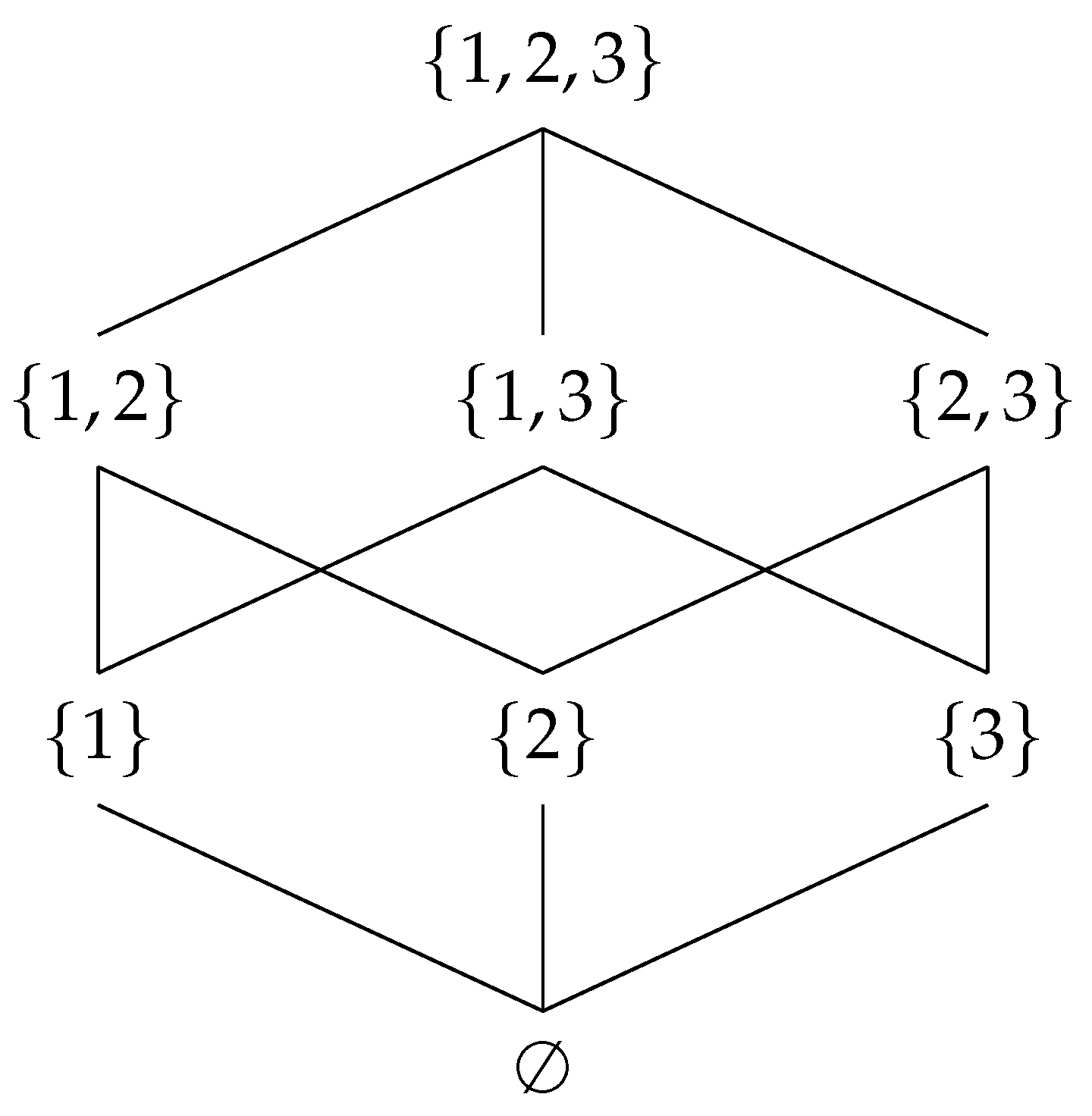
A Hasse diagram is a graphical representation of a finite partially ordered set, in which each element is represented by a node and each relationship between elements is represented by an edge connecting the vertices. The nodes are arranged in a hierarchy, with the elements that are related by a partial order being placed on a single line. The edges of the diagram are directed, pointing from the element that is lower in the partial order to the element that is higher in the partial order. A Hasse diagram example for a power set of a set $1,2,3$ is shown in Figure 1. The partial order in this instance is the subset–superset relation.

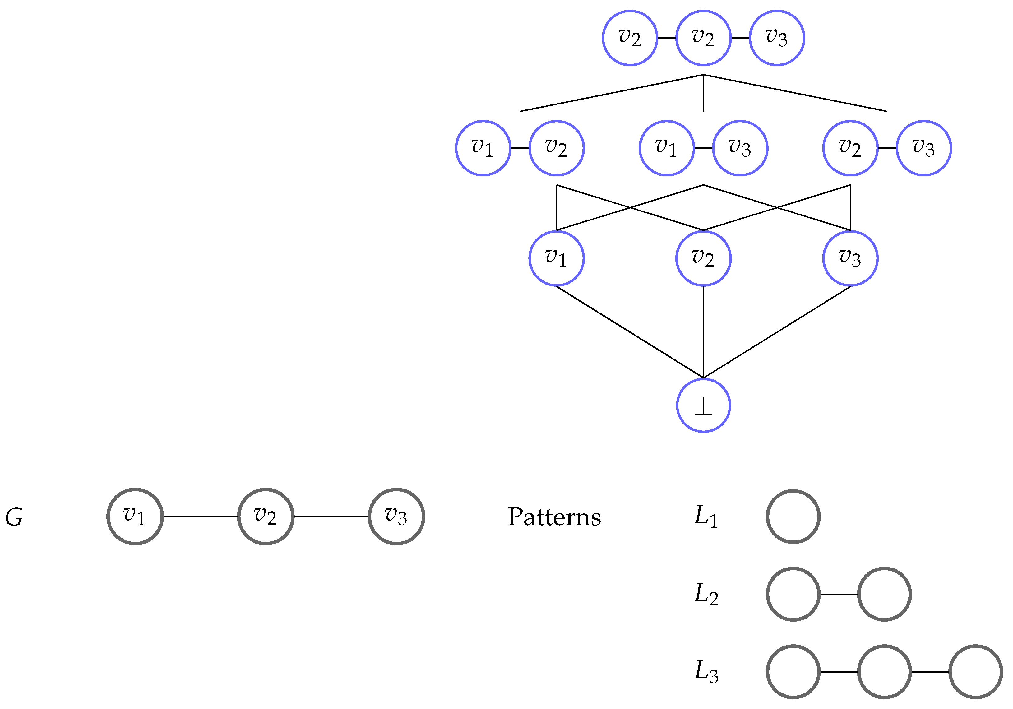
Using this concept, I define a flow network $\mathcal{N}$ for a single-graph database $G=(V,E)$ that is called an instance network as follows:

• The nodes of this network are instances of all the patterns in G, including the empty instance ⊥ and G itself.
• The empty instance is the bottom element of the diagram, and G is the top element.
• The edges of the network are defined by the Hasse diagram of the partially ordered set implied by the subgraph relation on pattern instances.
• All edge weights are set to 1.
• The empty instance ⊥ is considered to be a subgraph of all the nodes in V.

Example 1.

Figure 2 shows the instance network of a database graph G, which is an unlabeled path of length 2. It has three patterns, $L_1$, $L_2$, and $L_3$, that are unlabeled paths of length 1, 2, and 3, respectively. $L_1$ has three instances in G that are single nodes, $L_2$ has three different instances, and $L_1$ has one instance.

For a pattern, p, $\mathcal{N}\left[p\right]$ denotes the instance network defined on instances of p and its sub-patterns only.

In this paper, I rely on the following theorem proven in my previous work.

Theorem 2

([27]). Let M be a valid support measure, G be a database graph, and p a pattern in G. Then, there exists a node-disjoint flow $f_p$ in $\mathcal{N}\left[p\right]$ so that $|f_p|=M\left(p\right)$.

Given the connection between flows and support measures, I define a separate category for measures that correspond to max-flows in the following definition.

Definition 1.

A valid support measure M is maximal for pattern p in database G if the size of a max-flow in instance network $\mathcal{N}\left[p\right]$ is $M\left(p\right)$. A valid support measure M is maximal if it is maximal for all patterns p.

Note that any valid support measure can be extended to a maximal one by taking its corresponding flow in the instance network and extending it to a max-flow.

Additionally, I prove here some basic properties of maximal node-disjoint flows that will be used later.

Property 1.

Let p be a pattern, and $\mathcal{N}\left[p\right]$ its corresponding instance network of a database graph G. Let C be a node min-cut in $\mathcal{N}\left[p\right]$, and $f_{max}$ be a $(\perp ,G)$-flow saturating (i.e., traversing all the nodes of) cut C. Then, no two paths of $f_{max}$ intersect in a node different from ⊥ and G.

Proof. 

Assume the contrary and let two paths $P,Q\in f_{max}$, have a common node x. Let p and q be the nodes of C traversed by P and Q, respectively. Then, $C \backslash \{p,q\}\cup \left\{x\right\}$ is a node cut in $\mathcal{N}$ that is saturated by $f_{max} \backslash \left\{P\right\}$ of size $\left|C\right|-1$. This contradicts the assumption about C being a min-cut by Menger’s theorem.    □

Property 2.

Let p be a pattern, and $\mathcal{N}\left[p\right]$ its corresponding instance network. Let C be a node min-cut in $\mathcal{N}\left[p\right]$, and $f_{max}$ be a node-disjoint $(\perp ,G)$-flow saturating (i.e., traversing all the nodes of) C. Let path $P\in f_{max}$ traverse a node $x\in C$ and a node y lie on a segment $xPG$ of P. Then, $C \backslash \left\{x\right\}\cup \left\{y\right\}$ is a node min-cut in $\mathcal{N}$ as well.

Proof. 

Note that node set $C \backslash \left\{x\right\}\cup \left\{y\right\}$ is saturated by the paths of $f_{max}$ that do not intersect by Property 1, and its size is identical to the size of C.    □

3. Sufficient Instance Networks

For frequent graph patterns or those with support measures bigger than a user-defined parameter S, one is interested in computing valid graph measures when mining graphs, meaning that one must determine whether $M\left(p\right)$ is bigger than S for a given measure M. Theorem 2 states that for any valid measure M, a flow corresponding to $M\left(p\right)$ exists in the instance network N, allowing one to compute M using this network. However, when there are numerous patterns and instances and the database graph is dense, the size of a network N might be rather huge.

In this section, I demonstrate how N can be replaced by smaller instance network sub-networks. When using a certain graph mining algorithm, the obvious reason to seek a smaller network is to reduce the computation time of a reliable support measure. These algorithms have a propensity to iteratively construct graph patterns, but the precise sequence in which they appear varies from method to algorithm (e.g., [37,38,39,40,41]). The process of graph mining does not require a central element. Patterns are usually generated and tested for frequency in a bottom–up fashion, from smaller patterns to larger ones.

3.1. Definition

First, notation is provided below.

Definition 2.

Let $\mathcal{M}\subseteq \mathcal{N}$ be a sub-network of the instance network defined on instances of some patterns in G. Let M be a valid support measure. Then, $M(p,\mathcal{M})$ denotes the value of the measure M for pattern p computed from the network $\mathcal{M}$.

Super patterns of p are not necessary to compute the value of $M\left(p\right)$ by Theorem 2 if M is a valid support measure. As a result, we can declare the following right away.

Property 3.

Let p be a pattern and let ${\mathcal{N}}_{\mathit{smaller}}$ include the instances of p and its sub-patterns only. Then, $M(p,{\mathcal{N}}_{\mathit{smaller}})=M\left(p\right)$.

Following Property 3, I can introduce an extension of this concept.

Definition 3.

Let $\mathcal{M}$ be a sub-network of the instance network $\mathcal{N}$. $\mathcal{M}$ is called sufficient if for every valid support measure M, every pattern p, and every user-defined support threshold $S\ge 0$ holds

$$\begin{array}{c}M(p,\mathcal{M})\ge S if M\left(p\right)\ge S\hfill \\ M(p,\mathcal{M})<S if M\left(p\right)<S and M is maximal\hfill \end{array}$$

(1)

Definition 4.

A sub-network $\mathcal{M}$ is called sufficient for pattern p if Equation (1) holds for p.

Note that sufficiency is transitive because pruning a sufficient network with a filter according to Equation (1) preserves it.

3.2. Examples of Insufficient Sub-Networks

I list several counterexamples of sufficiency below to demonstrate that the notion of sufficiency is not straightforward. They serve to demonstrate that naive recommendations for adequate sub-network architecture are ineffective.

Counterexample 1.

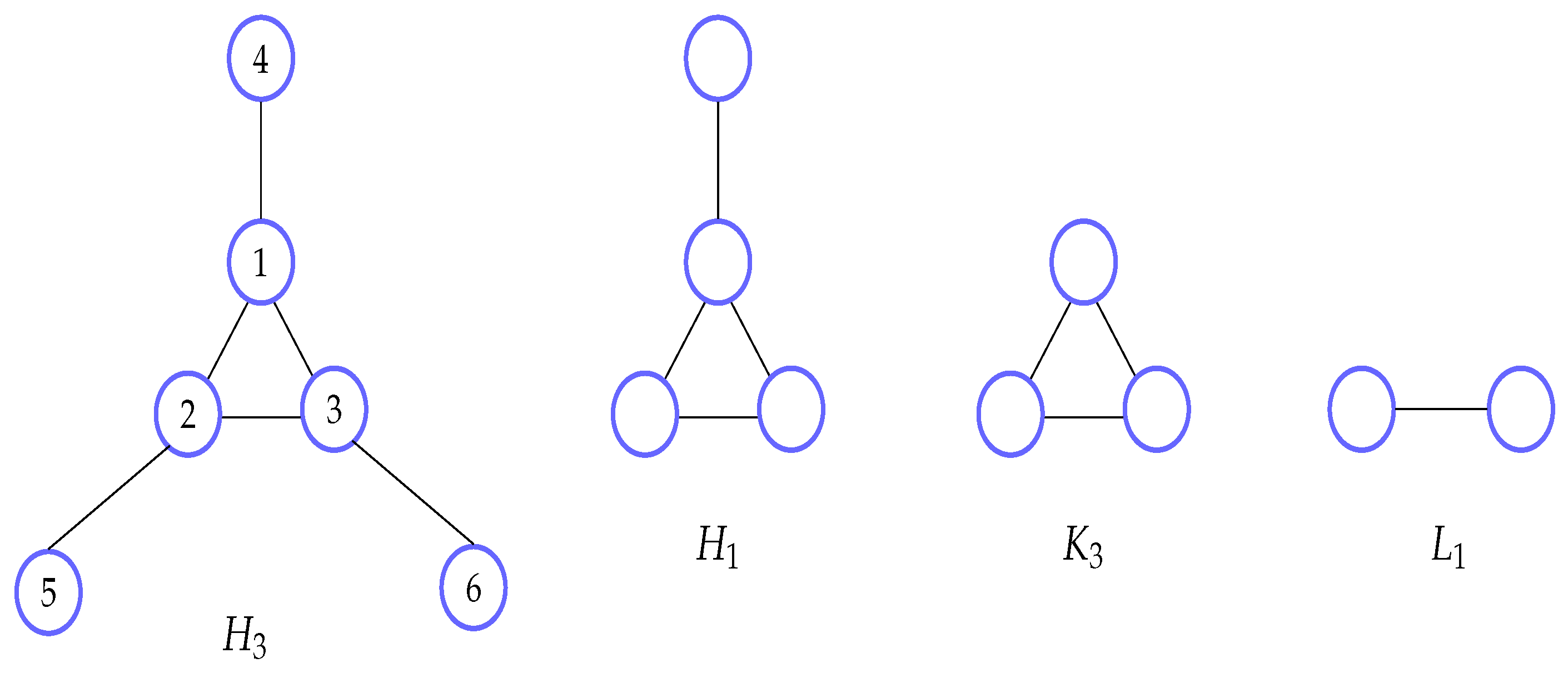
Graphs $g_1,\cdots ,g_n$ are said to cover graph g if the union of instances give us precisely the node and edge sets of g. Let p be a connected pattern in G. Sub-network ${\mathcal{N}}_{\mathit{cover}}$, which contains instances of patterns covering p, is not sufficient.

Proof. 

Observe an unlabeled pattern $H_3$ (for the ‘three horns’) depicted in Figure 3. In a setting where $G=H_3$, a subpattern $L_1$ (a single edge) of $H_3$ covers all other patterns, including $H_1$ and $K_3$. Let M be any maximal valid support measure. Clearly, $M\left(K_3\right)=1$ because $K_3$ has only one instance in G and therefore the size of a node min-cut in $\mathcal{N}\left[K_3\right]$ is 1. Then, $M\left(H_1\right)\le 1$ because $K_3$ is a subgraph of $H_1$ and M is anti-monotonic.

Let us define a sub-network ${\mathcal{N}}_{\mathit{cover}}$ to contain the instances of edge $L_1$ only (this network is shown in Figure 4). This network does not contain a node cut of size 1 separating G and ⊥, and thus by Menger’s theorem a max-flow corresponding to $M({\mathcal{N}}_{\mathit{cover}},K_3)$ has a size bigger than 1.    □

Because $K_3$ is still the bounding factor when computing any maximal valid measure for $H_1$, the same issue as in Counterexample 1 arises if one uses larger patterns encompassing $H_1$, such as paths of length 2.

It may seem that covering p with patterns similar to $K_3$ will provide a solution, but the next claim shows that is not true.

Counterexample 2.

Let p be a connected pattern in G and let ${\mathcal{N}}_{\mathit{complete},c}$ be a sub-network limited to instances of complete graphs $K_i$ of size no more than c. Then, ${\mathcal{N}}_{\mathit{complete},c}$ is not sufficient.

Proof. 

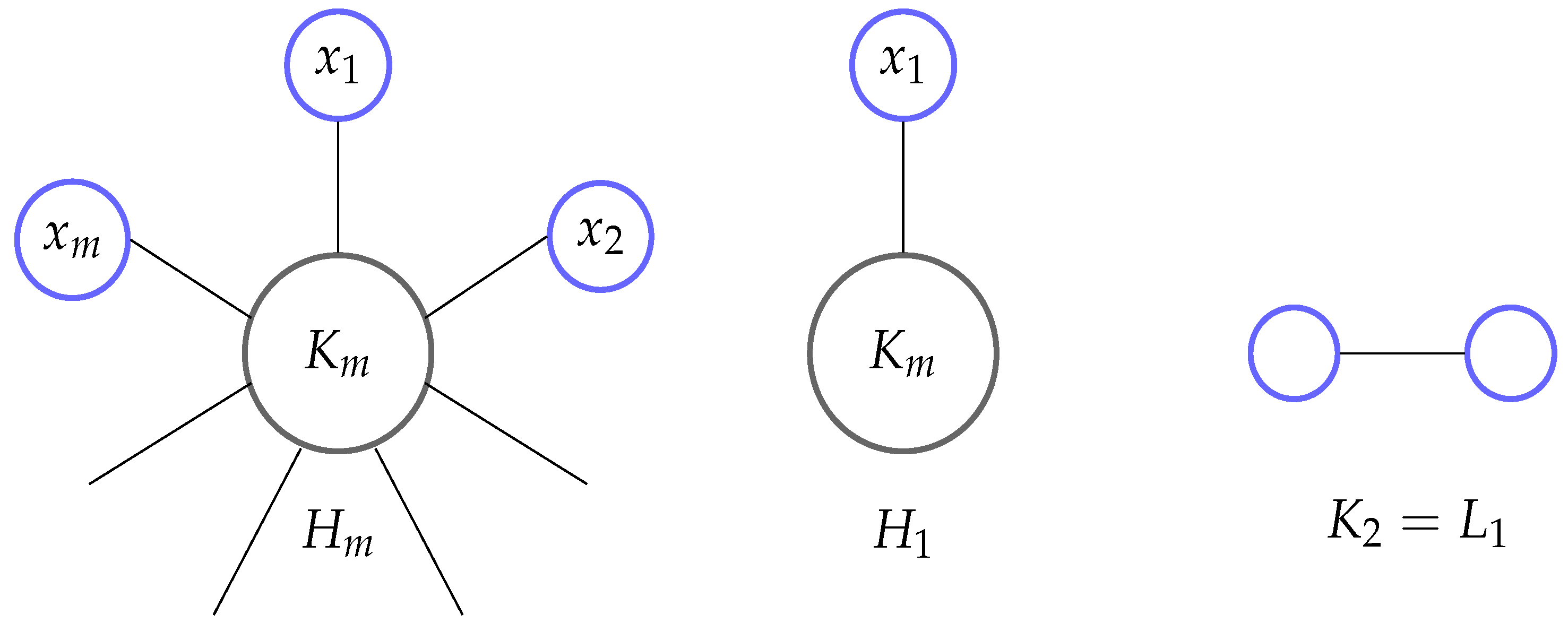
Observe a maximal valid measure M. Let $H_m$ (for ‘m horns’) be a pattern consisting of a complete graph $K_m$, $m>c$, and nodes $x_1,\cdots ,x_m$ of degree 1, each connected to a different node of $K_m$ (see Figure 5). A pattern $H_{m,1}$ consists of a complete graph $K_m$ and one degree 1 node connected to it.

Clearly, instances of all complete graphs $K_1,K_2,\cdots ,K_c$ cover both $H_m$ and $H_{m,1}$ in the data graph. However, $K_m$ itself has only one instance in the database graph that is not contained in ${\mathcal{N}}_{\mathit{complete},c}$.

Then, $M(H_{m,1},{\mathcal{N}}_{\mathit{complete},c})\ge 2$ because there are at least two instances of graphs $H_{c,1}$ that are the largest subgraphs of $H_{m,1}$ represented in ${\mathcal{N}}_{\mathit{complete},c}$ and thus the size of a node min-cut is at least 2. In the original network, however, $M\left(H_{m,1}\right)=1$. Therefore, ${\mathcal{N}}_{\mathit{complete},c}$ is not sufficient.    □

Even if a limit on the order of complete subgraphs is waived, sufficiency remains out of reach.

Counterexample 3.

Let $G=L_n$ denote a simple path with $n\ge 3$ edges. Let p be a connected pattern in G and let ${\mathcal{N}}_{\mathit{complete}}$ be the sub-network that contains instances of complete graphs of any order. Then, ${\mathcal{N}}_{\mathit{complete}}$ is not sufficient for $L_n$.

Proof. 

Because $G=L_n$, the only complete subgraphs with instances in G are $K_1$ and $K_2$. A pattern $L_n$ contains more than two disjoint copies of $K_2$ because $n-1\ge 3$. Then, ${\mathcal{N}}_{\mathit{complete}}$ contains no node cut of size 1, meaning that $M(L_n,{\mathcal{N}}_{\mathit{complete}})\ge 2$ for any maximal valid supports measure M. It contradicts (1) because there is only one instance of $L_n$ in the database and for support values $S\ge 2$, sufficiency requires that $M(L_n,{\mathcal{N}}_{\mathit{complete}})<2$.    □

3.3. Sufficient Networks

In this section, I prove sufficiency for several types of instance networks. Our first theorem addresses connected patterns. It is worth noting that most modern graph mining algorithms focus on connected patterns only.

Theorem 3.

Let ${\mathcal{N}}_{\mathit{conn}}$ be the sub-network of $\mathcal{N}$ containing the instances of connected patterns only. Then, ${\mathcal{N}}_{\mathit{conn}}$ is sufficient for all connected patterns.

Proof. 

Let p be a connected pattern in G and let M be a valid support measure.

Suppose first that $M\left(p\right)<S$ and M is maximal. Then, there exists no node-disjoint flow of size S in $\mathcal{N}\left[p\right]$, implying the existence of a node min-cut C in $\mathcal{N}\left[p\right]$ of size $\left|C\right|<S$.

Case 1: C contains instances of connected patterns only. Then, C is a cut in ${\mathcal{N}}_{\mathit{conn}}\left[p\right]$ as well. This cut prevents the existence of flows of a size larger than $\left|C\right|$ in ${\mathcal{N}}_{\mathit{conn}}$, meaning that $M\left(p\right)<S$ by Theorem 2.

Case 2: C contains at least one instance of a disconnected pattern. Let $f_{max}$ be a maximal edge-disjoint flow in $\mathcal{N}\left[p\right]$ that saturates C, and let $P\in f_{max}$ be a path that traverses a disconnected instance $x\in C$. Because P traverses a single instance $p_j$ of p that is connected by definition, we can replace x by $p_j$ in C by Property 2. Thus, one can assume that C contains connected instances only and we have the previous case.

Suppose now that $M\left(p\right)\ge S$. Let $f_{max}$ be a maximal flow in $\mathcal{N}\left[p\right]$ that saturates a node min-cut C. Then, $\left|C\right|\ge M\left(p\right)\ge S$ by Theorem 2. Observe a path $P\in f_{max}$. If all instances traversed by P are connected, this path exists in ${\mathcal{N}}_{\mathit{conn}}\left[p\right]$ as well. Otherwise, P contains at least one disconnected instance. Let $xPy$ denote the segment of P whose start x and end y are connected instances, and the inner nodes are disconnected instances. Because x is a subgraph of y, there exists a path $x,z_1,\cdots ,z_k,y$ in $\mathcal{N}\left[p\right]$ such that all $z_i$ are connected instances. For example, one can take $z_1$ to be a union of x and a spanning tree of y and then add edges until one obtains y. Replace the segment $xPy$ in path P with a new segment $x,z_1,\cdots ,z_k,y$ and obtain a new path $P^{\prime }$. Flow $f_{max}^{\prime }:=f_{max} \backslash \left\{P\right\}\cup \left\{P^{\prime }\right\}$ has the same size as $f_{max}$ and is therefore a maximal flow in $\mathcal{N}\left[p\right]$ that saturates C. Then, by Property 2, its paths do not intersect. Thus, one can always select the paths of $f_{max}$ to contain connected instances only, meaning that this flow of size at least S exists in ${\mathcal{N}}_{\mathit{conn}}$. Then, $M(p,{\mathcal{N}}_{\mathit{conn}})\ge S$ as well, as required.    □

The theorem below and its corollaries describe additional classes of patterns of sufficient networks.

Theorem 4.

Let $\mathcal{C}$ be a class of graph patterns closed under inclusion, meaning that subgraph isomorphism $q⊏p$ implies that either $q\in \mathcal{C}$ or q is a single node. Then, the sub-network ${\mathcal{N}}_{\mathcal{C}}$ limited to instances of patterns in $\mathcal{C}$ is sufficient for all the patterns in $\mathcal{C}$. Moreover, the value of a valid support measure in this network is identical to the original.

Proof. 

Let p be a connected pattern in G and let M be a valid support measure. By Theorem 2 there exists a flow f of size $\left|f\right|=M\left(p\right)$ in $\mathcal{N}\left[p\right]$. Any path $P\in f$ traverses instances of sub-patterns of p that are contained in $\mathcal{C}$ because $\mathcal{C}$ is closed under inclusion. Therefore, the flow f exists in the network ${\mathcal{N}}_{\mathcal{C}}\left[p\right]$ too, meaning that $M(p,{\mathcal{N}}_{\mathcal{C}})\ge M\left(p\right)$.

Similarly, let P be a path of a flow g in ${\mathcal{N}}_{\mathcal{C}}\left[p\right]$ and let $(x,y)$ be an edge of P. If this edge does not exist in $\mathcal{N}\left[p\right]$, then $\mathcal{N}\left[p\right]$ contains a path Q from x to y because x is a subgraph of y. However, $\mathcal{C}$ is closed under inclusion, and any instance traversed by Q lies in $\mathcal{C}$, meaning that it is present in network ${\mathcal{N}}_{\mathcal{C}}\left[p\right]$ as well. But then Q exists in ${\mathcal{N}}_{\mathcal{C}}\left[p\right]$ and thus an edge $(x,y)$ cannot exist there because the network is a Hasse diagram. Therefore $M(p,{\mathcal{N}}_{\mathcal{C}})\le M\left(p\right)$. Therefore, we have $M(p,{\mathcal{N}}_{\mathcal{C}})=M\left(p\right)$ and thus sufficiency holds.    □

Corollary 1.

Any class of graphs with forbidden minors satisfies Theorem 4. This includes planar graphs and graphs of bounded treewidth.

Corollary 2.

Trees satisfy the condition of Theorem 4.

Proof. 

By Theorem 3 and transitivity of sufficiency, we can limit the network to connected subgraphs of trees, which are trees as well.    □

Because any valid support measure M is anti-monotonic, $M\left(p\right)\ge S$ implies that $M\left(q\right)\ge S$ for any $q⊏p$. Therefore, frequent patterns are closed under inclusion and the following can be deduced.

Corollary 3.

Let the network ${\mathcal{N}}_{\mathit{freq}}$ contain only the instances of frequent patterns. Then, ${\mathcal{N}}_{\mathit{freq}}$ is sufficient.

Joining Theorem 3 and Corollary 3 together and using a transitivity of sufficiency, the following corollary arises.

Corollary 4.

Let ${\mathcal{N}}_{\mathit{freq},\mathit{conn}}$ be the sub-network containing only the instances of frequent connected patterns. Then, ${\mathcal{N}}_{\mathit{freq},\mathit{conn}}$ is sufficient for any connected pattern p.

4. Intersection Networks

In this section, I describe instance networks that can be utilized to compute a valid support measure for a given pattern directly from the database graph.

Let G be a database graph, p a pattern in that graph, and $\mathcal{N}$ the instance network corresponding to G. Let $\mathit{inst}\left(p\right)=p_1,\cdots ,p_n$ be the instances of p in G. Observe a set of patterns contained in intersections of these instances:

$$\mathit{Int}=\bigcup _{1\le i<j\le n}{p}_i\cap p_j\cup V$$

Definition 5.

The intersection network ${\mathcal{N}}_{\mathit{intersect}}\left[p\right]$ is the sub-network of $\mathcal{N}$ that contains ⊥, the database graph G, the instances of p, the instances of all the patterns in the set $\mathit{Int}$, and the instances of their sub-patterns.

This network is far smaller than $\mathcal{N}$ as a whole.

Sufficiency

Next, I prove the sufficiency of intersection networks.

Theorem 5.

Network ${\mathcal{N}}_{\mathit{intersect}}\left[p\right]$ is sufficient for p.

Proof. 

Let p be a connected pattern in G, M be a valid support measure and S be a support boundary. By Theorem 2 there exists a flow f of size $\left|f\right|=M\left(p\right)$ in $\mathcal{N}\left[p\right]$.

Assume first that $M\left(p\right)\ge S$. If ${\mathcal{N}}_{\mathit{intersect}}\left[p\right]$ has no flow of size $M\left(p\right)$ or bigger, then it contains a node min-cut C of size $\left|C\right|<M\left(p\right)$. The cut C contains instances of sub-patterns of p that lie in $\mathit{Int}$. But then C is a cut for a network $\mathcal{N}\left[q\right]$ for some subpattern q of p such that $q\in \mathit{Int}$. Because M is valid and thus anti-monotonic, $M\left(q\right)\ge M\left(p\right)$ and by Theorem 2 there exists a flow of size $M\left(q\right)$ in $\mathcal{N}\left[q\right]$, which is a contradiction to C being a node-cut in $\mathcal{N}\left[q\right]$.

Assume now that $M\left(p\right)<S$ and M is maximal, meaning that a node cut C of size $\left|C\right|<S$ exists in $\mathcal{N}\left[p\right]$.

• Case 1: if C contains nodes, instances of p and instances of patterns in $\mathit{Int}$, it exists in network ${\mathcal{N}}_{\mathit{intersect}}\left[p\right]$ as well and then $M(p,{\mathcal{N}}_{\mathit{intersect}})<S$ as well because there is no flow of size S or bigger in ${\mathcal{N}}_{\mathit{intersect}}\left[p\right]$.
• Case 2: otherwise, C contains instances of patterns $q_1,\cdots ,q_k\notin \mathit{Int}$. Then, every instance $q_i^{\mathit{instance}}$ of $q_i$ in C is a subgraph of a different instance of p, denoted by $p_i$. If this is not the case then $q_i^{\mathit{instance}}$ lies in an intersection of two instances of p and we have $q_i\in \mathit{Int}$ contrary to our assumption. Let us replace in C every such instance $q_i^{\mathit{instance}}$ by the instance $p_i$ of p and have case 1.

□

Next, observe an even smaller network that contains only inclusion-maximal intersections of instances of p. Define the set ${\mathit{Int}}_{max}$ to be a subset of $\mathit{Int}$ where $x\in {\mathit{Int}}_{max}$ if and only if there exists a pair of instances $p,q\in \mathit{inst}\left(p\right)$ such that $x\sim p\cap q$.

Definition 6.

The intersection network ${\mathcal{N}}_{\mathit{intersect}}^{max}\left[p\right]$ is the sub-network of $\mathcal{N}$ that contains ⊥, the database graph G, the instances of p, and the instances of all the patterns in the set of inclusion-maximal patterns ${\mathit{Int}}_{max}$.

Corollary 6.

Network ${\mathcal{N}}_{\mathit{intersect}}^{max}\left[p\right]$ is sufficient for p.

Proof. 

Let p be a connected pattern in G, M be a valid support measure and S be a support boundary. By Theorem 2 there exists a flow f of size $\left|f\right|=M\left(p\right)$ in $\mathcal{N}\left[p\right]$.

The case of $M\left(p\right)\ge S$ is identical to Theorem 5. If $M\left(p\right)<S$ and M is maximal, then a node cut C of size $\left|C\right|<S$ exists in $\mathcal{N}\left[p\right]$. If C is a cut in ${\mathcal{N}}_{\mathit{intersect}}\left[p\right]$ as well, meaning that C is a subset of $V\cup \mathit{inst}\left(p\right)\cup {\mathit{Int}}_{max}$, then $M(p,{\mathcal{N}}_{\mathit{intersect}}^{max})<S$ by Menger’s theorem. Otherwise, C contains instances $q_1,\cdots ,q_k\notin {\mathit{Int}}_{max}$. If these instances are not contained in $\mathit{Int}$ either, we have the case identical to Theorem 5. Otherwise, let $q_i\in \mathit{Int} \backslash {\mathit{Int}}_{max}$. Let P be a path of max-flow $f_{max}$ in $\mathcal{N}\left[p\right]$ that saturates C and traverses $q_i$. Then, P traverses an instance $r_i\in {\mathit{Int}}_{max}$ by the definition of ${\mathit{Int}}_{max}$. Replace $q_i$ by $r_i$ in C and do so for all non-maximal instances in C; it is possible because the paths of $f_{max}$ are node-disjoint. Then, we have the previous case.    □

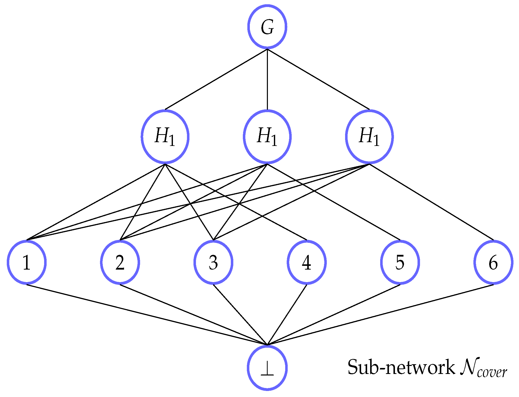
Maximal intersection networks are minimal in the sense that in general, omitting even one maximal intersection pattern results in an insufficient instance network. As an illustration, if one looks at database graph $H_m$ and sees pattern $H_1$, the only maximal intersection pattern for its instances is $K_m$ (shown in Figure 5). The single node-cut in the instance network with a size of 1 is eliminated when this pattern is skipped, and a maximal valid support measure for this pattern will then have a value of ≥2.

Next, I offer a method for computing a reliable support metric for a graph pattern using maximal intersection networks. Using Corollary 6, this approach uses only the instances of p to reconstruct the necessary portion of the instance network. Therefore, one just needs to look at the sub-network ${\mathcal{N}}_{\mathit{intersect}}^{max}$ of these patterns and their sub-patterns for a pattern p. The top–down construction used in this method is described in Algorithm 1.

Algorithm 1 Computing maximal support measures from ${\mathcal{N}}_{\mathit{intersect}}^{max}\left[p\right]$

Require:  database graph $G=(V,E)$, pattern p, valid support measure M. Ensure:  $M({\mathcal{N}}_{\mathit{intersect}}^{max},p)$ 1:   2: function$IntersectionNetwork$(G,p) 3:     Initialize ${\mathcal{N}}_{\mathit{intersect}}^{max}\left[p\right]$ with G, V, ⊥, and $\mathit{inst}\left(p\right)$ 4:     for $p,q\in \mathit{inst}\left(p\right)$ do 5:         if $q\ne p$ then 6:            Add to ${\mathcal{N}}_{\mathit{intersect}}^{max}\left[p\right]$ all instances of $p\cap q$ 7:         end if 8:     end for 9:     return ${\mathcal{N}}_{\mathit{intersect}}^{max}\left[p\right]$ 10: end function 11:   12: ${\mathcal{N}}_{\mathit{intersect}}\leftarrow \mathit{IntersectionNetwork}(G,p)$ 13: if${\mathcal{N}}_{\mathit{intersect}}\ne \varnothing$then 14:     return $M(p,{\mathcal{N}}_{\mathit{intersect}})$ 15: else 16:     return $\left|\mathit{inst}\right(p\left)\right|$ 17: end if

5. Experimental Evaluation

5.1. Graph Types and Objectives of Experiments

The testing was conducted on synthetic graphs of three types: Erdős–Rényi graphs (with default density 0.5), complete graphs (denoted by $K_n$), and balanced complete bipartite graphs (denoted by $K_{n,n}$). Density of an undirected graph $G=(V,E)$ is measured as

$$\mathit{density}\left(G\right)=\frac{\left|E\right|}{\left|V\right|·\left(\right|V|-1)}$$

Queries in all cases were random Erdős–Rényi graphs of orders 10 to 20; even sizes only were used for complete bipartite graphs. Experiments evaluated sizes of several instance network types: (1) the complete network $\mathcal{N}$, (2) the network ${\mathcal{N}}_{\mathit{conn}}$ containing connected patterns only, and (3) the intersection network ${\mathcal{N}}_{\mathit{intersect}}$. The purpose of experimental assessment was multifold:

• To study whether or not using ${\mathcal{N}}_{\mathit{conn}}$ instead of $\mathcal{N}$ decreases the network size;
• To evaluate the effect of graph density on network size when using ${\mathcal{N}}_{\mathit{conn}}$;
• To study how the use of an intersection network for a specific pattern affects the network size.

5.2. Software and Hardware Setup

Experiments were performed on Google Colab [42] with Pro settings. The code was written in Python using the networkX package [43] for graph generation, graph isomorphism, and subgraph isomorphism testing.

5.3. Evaluation Results

Table 1. Instance network size comparison for $\mathcal{N}$ and ${\mathcal{N}}_{\mathit{conn}}$.

Graph	Nodes	Edges	$\left|\mathcal{N}\right|$	$|{\mathcal{N}}_{\mathit{conn}}|$	$|{\mathcal{N}}_{\mathit{conn}}|/\left|\mathcal{N}\right|$ Ratio
Erdős–Rényi	10	20	$1.0486\times {10}^6$	576	$5.4932\times {10}^{-4}$
Erdős–Rényi	11	26	$6.7109\times {10}^7$	1496	$2.2292\times {10}^{-5}$
Erdős–Rényi	12	30	$1.0737\times {10}^9$	3066	$2.8554\times {10}^{-6}$
Erdős–Rényi	13	34	$1.7180\times {10}^{10}$	6265	$3.6467\times {10}^{-7}$
Erdős–Rényi	14	41	$2.1990\times {10}^{12}$	13,561	$6.1668\times {10}^{-9}$
Erdős–Rényi	15	56	$7.2058\times {10}^{16}$	30,517	$4.2351\times {10}^{-13}$
Erdős–Rényi	16	55	$3.6029\times {10}^{16}$	57,956	$1.6086\times {10}^{-12}$
Erdős–Rényi	17	68	$2.9515\times {10}^{20}$	121,646	$4.1215\times {10}^{-16}$
Erdős–Rényi	18	74	$1.8889\times {10}^{22}$	247,486	$1.3102\times {10}^{-17}$
Erdős–Rényi	19	85	$3.8686\times {10}^{25}$	497,709	$1.2865\times {10}^{-20}$
Erdős–Rényi	20	102	$5.0706\times {10}^{30}$	1,031,828	$2.0349\times {10}^{-25}$
$K_n$	10	45	$3.5184\times {10}^{13}$	1023	$2.9075\times {10}^{-11}$
$K_n$	11	55	$3.6029\times {10}^{16}$	2047	$5.6816\times {10}^{-14}$
$K_n$	12	66	$7.3787\times {10}^{19}$	4095	$5.5498\times {10}^{-17}$
$K_n$	13	78	$3.0223\times {10}^{23}$	8191	$2.7102\times {10}^{-20}$
$K_n$	14	91	$2.4759\times {10}^{27}$	16,383	$6.6170\times {10}^{-24}$
$K_n$	15	105	$4.0565\times {10}^{31}$	32,767	$8.0777\times {10}^{-28}$
$K_n$	16	120	$1.3292\times {10}^{36}$	65,535	$4.9303\times {10}^{-32}$
$K_n$	17	136	$8.7112\times {10}^{40}$	131,071	$1.5046\times {10}^{-36}$
$K_n$	18	153	$1.1418\times {10}^{46}$	262,143	$2.2959\times {10}^{-41}$
$K_n$	19	171	$2.9932\times {10}^{51}$	524,287	$1.7516\times {10}^{-46}$
$K_n$	20	190	$1.5693\times {10}^{57}$	1,048,575	$6.6819\times {10}^{-52}$
$K_{n/2,n/2}$	10	25	$3.3554\times {10}^7$	971	$2.8938\times {10}^{-5}$
$K_{n/2,n/2}$	12	36	$6.8719\times {10}^{10}$	3981	$5.7931\times {10}^{-8}$
$K_{n/2,n/2}$	14	49	$5.6295\times {10}^{14}$	16,143	$2.8676\times {10}^{-11}$
$K_{n/2,n/2}$	16	64	$1.84467\times {10}^{19}$	65,041	$3.5259\times {10}^{-15}$
$K_{n/2,n/2}$	18	81	$2.41785\times {10}^{24}$	261,139	$1.0800\times {10}^{-19}$
$K_{n/2,n/2}$	20	100	$1.26765\times {10}^{30}$	1,046,549	$8.2558\times {10}^{-25}$

shows the sizes of full instance networks $\mathcal{N}$ and ${\mathcal{N}}_{\mathit{conn}}$ that were generated for the three types of graphs. Graph sizes vary from 10 to 20 nodes. In the final column, the ratio of instance network sizes is displayed. Since the ratios are tiny and the number of instances rises quickly, they are shown in exponential form. As can be seen, the ratio $|{\mathcal{N}}_{\mathit{conn}}|/\left|\mathcal{N}\right|$ decreases as graph size increases. This growth is more noticeable for denser graphs, such as complete graphs.

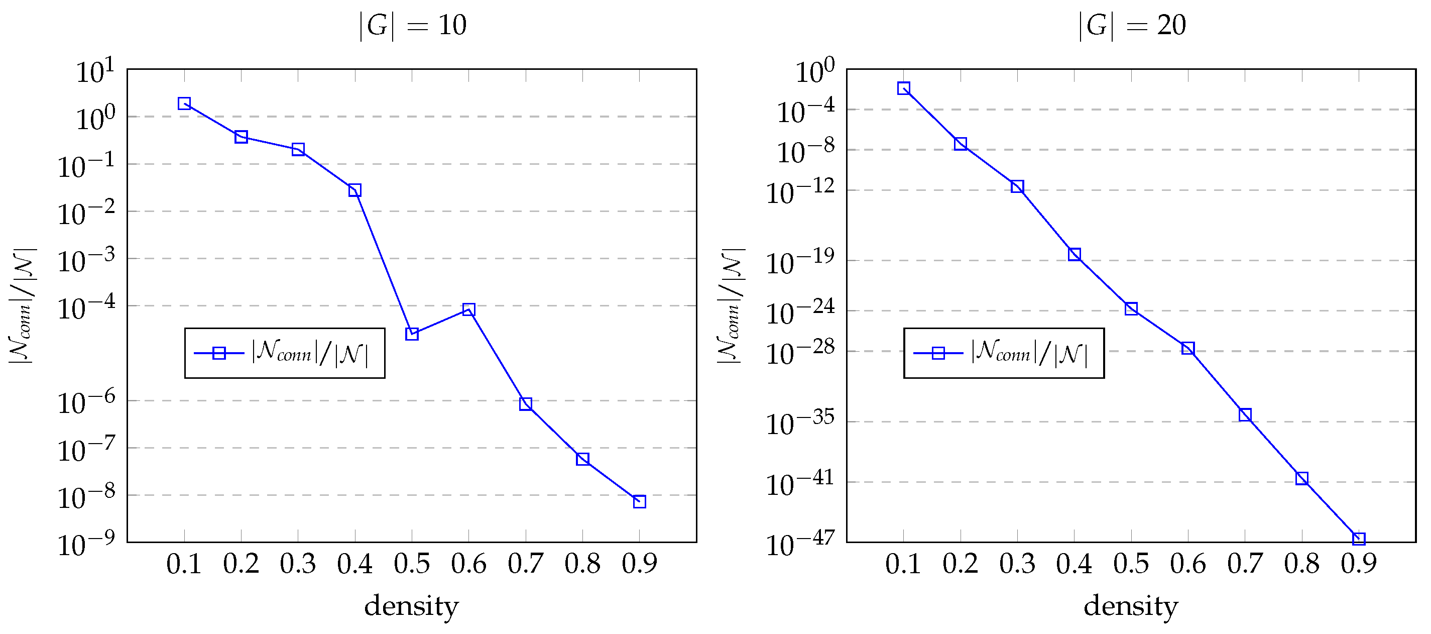
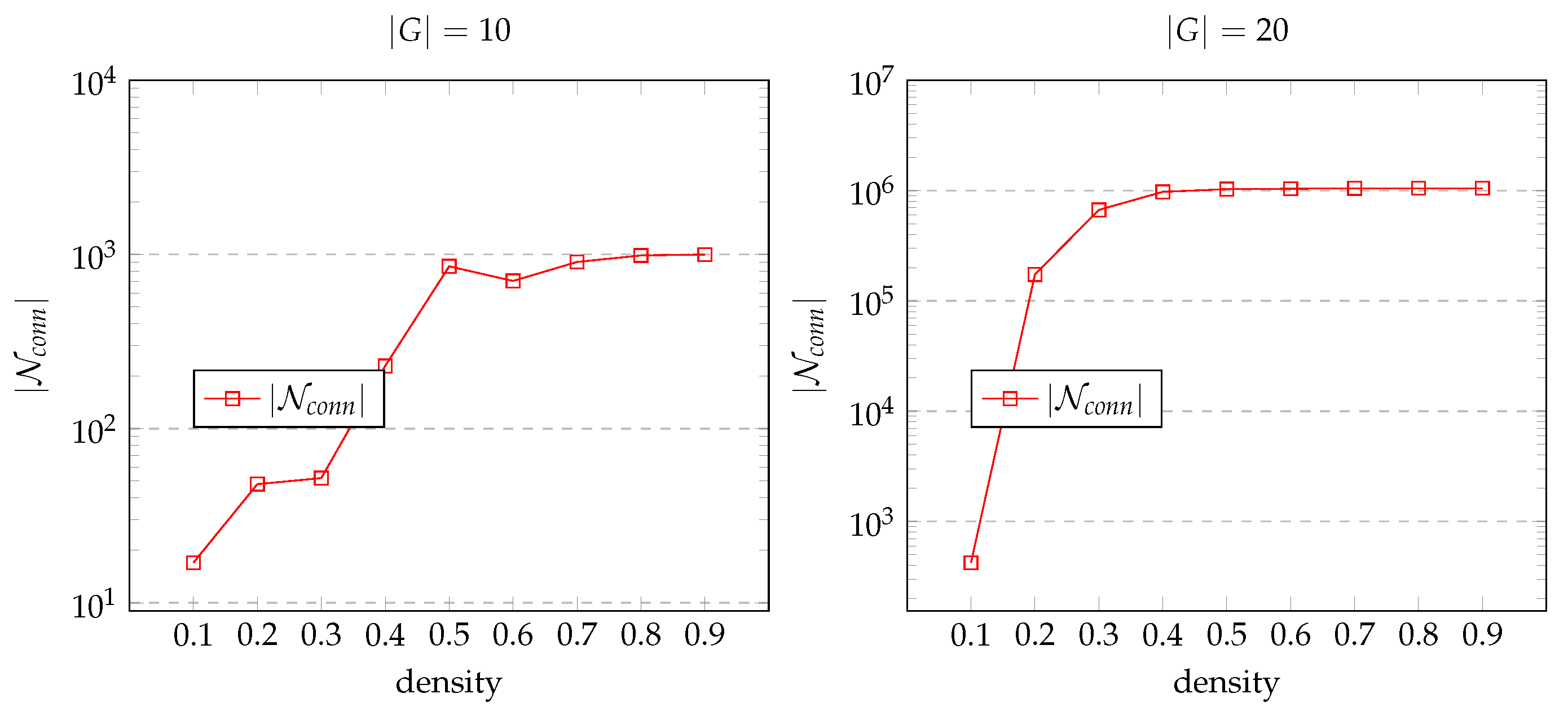
Charts in Figure 6 show how the ratio of sizes $\mathcal{N}$ and ${\mathcal{N}}_{\mathit{conn}}$ varies. For Erdős–Rényi random graphs of various densities, the charts in Figure 7 show dependency of ${\mathcal{N}}_{\mathit{conn}}$ size on graph density for graphs of size 10 and 20. The finding unmistakably demonstrates that as the database graph becomes denser, employing the ${\mathcal{N}}_{\mathit{conn}}$ instance network offers more significant benefits.

Table 2. Sizes of $\mathcal{N}\left[p\right]$ for patterns p on Erdős–Rényi graphs.

# of Graph	# of Graph	# of Pattern	# of Pattern	Size of	# of Pattern
Nodes	Edges	Nodes	Edges	$\mathcal{N}\left[\mathit{p}\right]$	Instances
25	141	5	6	$1.0247\times {10}^{10}$	2752
25	141	6	4	$1.6245\times {10}^7$	3032
25	141	7	9	$5.0141\times {10}^{13}$	1693
25	141	8	16	$5.5117\times {10}^{20}$	136
25	141	9	23	$1.9373\times {10}^{26}$	1
25	141	10	17	$4.0944\times {10}^{21}$	2
25	141	11	26	$2.0661\times {10}^{28}$	0
25	141	12	32	$7.0010\times {10}^{31}$	0
25	141	13	38	$5.7118\times {10}^{34}$	0
25	141	14	45	$2.9213\times {10}^{37}$	0
30	225	5	6	$1.7319\times {10}^{11}$	9141
30	225	6	8	$1.4909\times {10}^{14}$	13,144
30	225	7	11	$1.5406\times {10}^{18}$	1339
30	225	8	14	$6.9244\times {10}^{21}$	933
30	225	9	18	$1.8567\times {10}^{26}$	85
30	225	10	26	$9.0937\times {10}^{33}$	1
30	225	11	28	$4.8019\times {10}^{35}$	0
30	225	12	32	$8.3537\times {10}^{38}$	0
30	225	13	43	$4.1064\times {10}^{46}$	0
30	225	14	50	$4.5124\times {10}^{51}$	0

shows how the size of instance network $\mathcal{N}\left[p\right]$ changes with the growth of $\left|p\right|$. Both database graph G and patterns p are Erdős–Rényi unlabeled random graphs. For $\left|G\right|=35$ and larger, the search becomes infeasible in our experimental setting.

The size comparison for the full instance network $\mathcal{N}\left[p\right]$ and intersection network ${\mathcal{N}}_{\mathit{intersect}}\left[p\right]$ for various sizes of a pattern p is shown in

Table 3. Comparison of $\left|\mathcal{N}\right[p\left]\right|$ and $|{\mathcal{N}}_{\mathit{intersect}}\left[p\right]|$ for Erdős–Rényi graphs.

# of Graph	# of Graph	# of Pattern	# of Pattern	Size of	Size of	Ratio
Nodes	Edges	Nodes	Edges	$\mathcal{N}\left[\mathit{p}\right]$	${\mathcal{N}}_{\mathit{intersect}}\left[\mathit{p}\right]$	$|{\mathcal{N}}_{\mathit{intersect}}\left[\mathit{p}\right]|/\left|\mathcal{N}\right[\mathit{p}\left]\right|$
25	150	5	7	$3.09019\times {10}^{11}$	3139	$1.0158\times {10}^{-8}$
25	150	6	6	$1.49090\times {10}^9$	3648	$2.4468\times {10}^{-7}$
25	150	7	13	$2.01888\times {10}^{18}$	1297	$6.4244\times {10}^{-16}$
25	150	8	16	$1.55251\times {10}^{21}$	181	$1.1659\times {10}^{-19}$
25	150	9	15	$1.82322\times {10}^{20}$	44	$2.4133\times {10}^{-19}$
25	150	10	25	$2.43387\times {10}^{28}$	27	$1.1093\times {10}^{-27}$
25	150	11	28	$2.44802\times {10}^{30}$	27	$1.1029\times {10}^{-29}$
25	150	12	33	$2.28816\times {10}^{33}$	27	$1.1800\times {10}^{-32}$
25	150	13	42	$4.93515\times {10}^{37}$	27	$5.4710\times {10}^{-37}$
25	150	14	56	$1.71663\times {10}^{42}$	27	$1.5728\times {10}^{-41}$
30	224	5	2	$2.52020\times {10}^4$	1542	$6.1186\times {10}^{-2}$
30	224	6	8	$1.43811\times {10}^{14}$	7135	$4.9614\times {10}^{-11}$
30	224	7	9	$3.46866\times {10}^{15}$	2223	$6.4088\times {10}^{-13}$
30	224	8	11	$1.46565\times {10}^{18}$	320	$2.1833\times {10}^{-16}$
30	224	9	23	$1.54009\times {10}^{31}$	137	$8.8956\times {10}^{-30}$
30	224	10	19	$1.8635\times {10}^{27}$	32	$1.7172\times {10}^{-26}$
30	224	11	21	$1.87748\times {10}^{29}$	32	$1.7044\times {10}^{-28}$
30	224	12	38	$1.74807\times {10}^{43}$	32	$1.8306\times {10}^{-42}$
30	224	13	32	$7.17287\times {10}^{38}$	32	$4.4613\times {10}^{-38}$
30	224	14	50	$3.99394\times {10}^{50}$	32	$8.0121\times {10}^{-50}$

. Patterns p and database graph G are both Erdős–Rényi unlabeled random graphs. Due to the necessity of including all of the nodes in G, G itself, and the empty node ⊥, it should be noted that the minimum size of any instance network in this scenario is $\left|G\right|+2$. The ratio of instance network sizes is displayed in the last column.

Table 4. Comparison of $\left|\mathcal{N}\right[p\left]\right|$ and $|{\mathcal{N}}_{\mathit{intersect}}\left[p\right]|$ for Erdős–Rényi graphs with different number of labels and $\left|p\right|=5$.

# of	# of Graph	# of Graph	# of Pattern	# of Pattern	Size of	Size of	Ratio
Labels	Nodes	Edges	Nodes	Edges	$\mathcal{N}\left[\mathit{p}\right]$	${\mathcal{N}}_{\mathit{intersect}}\left[\mathit{p}\right]$	$|{\mathcal{N}}_{\mathit{intersect}}\left[\mathit{p}\right]|/\left|\mathcal{N}\right[\mathit{p}\left]\right|$
1	25	149	5	3	$5.5145\times {10}^5$	1644	$2.9812\times {10}^{-3}$
2	25	157	5	6	$1.9654\times {10}^{10}$	277	$1.4094\times {10}^{-8}$
3	25	140	5	3	$4.5745\times {10}^5$	53	$1.1586\times {10}^{-4}$
4	25	148	5	6	$1.3745\times {10}^{10}$	38	$2.7647\times {10}^{-9}$
5	25	149	5	8	$5.2715\times {10}^{12}$	27	$5.1219\times {10}^{-12}$
1	30	217	5	5	$3.9195\times {10}^9$	8380	$2.1380\times {10}^{-6}$
2	30	217	5	2	$2.3655\times {10}^4$	56	$2.3674\times {10}^{-3}$
3	30	224	5	5	$4.5970\times {10}^9$	40	$8.7013\times {10}^{-9}$
4	30	230	5	4	$1.1561\times {10}^8$	36	$3.1139\times {10}^{-7}$
5	30	234	5	6	$2.1947\times {10}^{11}$	32	$1.4580\times {10}^{-10}$

shows size comparison for the full instance network $\mathcal{N}\left[p\right]$ and intersection network ${\mathcal{N}}_{\mathit{intersect}}\left[p\right]$ for labeled graphs. The size of a pattern is fixed ($\left|p\right|=5$). Both the database graph and patterns are Erdős–Rényi random graphs with randomly assigned node labels, with the number of labels being in the range $1.5$. The ratio of instance network sizes is shown in the last column. One can see that all network sizes decrease as the number of labels increases, but the sizes of intersection networks are still significantly smaller.

6. Extensions and Limitations

The approach presented in this paper can be extended to the following types of graphs.

• Directed graphs.
  In this case, patterns and their instances are directed graphs as well, and the instance network is defined in the same way as for the undirected graphs. Therefore, Theorem 2 holds for directed graphs as well, and all the results in this paper apply to them.
• Edge and node labeled graphs.
  Node and edge labels affect how instances of graph patterns are found in the database graphs because subgraph isomorphism has to take label matching into account. However, the rest of the results are not affected. Table 4 shows some experimental evaluations I performed for this type of graph.
• Multi-graphs and graphs with integer edge weights.
  An integer edge weight w is equivalent to replacing that edge with w edges between its incident nodes. In both cases, the subgraph isomorphism test for pattern instances is affected, because of the number of edges between a pair of nodes taken into account. The rest of the results hold for these graph types.
• Graphs with real edge weights.
  This case is equivalent to the previous one.

The main limitation of the presented approach is that it does not address extensions of subgraph isomorphism, such as graph homomorphism, and less-than-or-equal edge matching for a real edge-weighted graph. For example, a graph $G_1=\{V=\{1,2\},E=\left\{\{1,2\}\right\},w\left(\{1,2\}\right)=2\}$ can be considered a subgraph of $G_2=\{V=\{1,2\},E=\left\{\{1,2\}\right\},w\left(\{1,2\}\right)=2.5\}$, and they cannot be reduced to multigraphs. In this case, Theorem 2 needs to be extended, and the instance network (in the form it is currently defined) is not suitable for representing support measures.

7. Conclusions

In this paper, I demonstrate how instance network sub-networks can be used to compute valid support measures for graph patterns. This concept has been incorporated into several graph mining methods, but because it is frequently entangled with the techniques themselves, each algorithm and each supporting measure must have its proof. Before the connection between flows and support measures was established in Theorem 2 in my prior work, it was impossible to verify these types of broad statements. This relationship means that a proving effort only needs to be made once, and this is the main result of this paper.

I demonstrate that smaller networks restricted to connected patterns, patterns with forbidden minors, or pattern intersections can be employed in place of larger networks when computing the support measure of a pattern. Additionally, I carried out an experimental evaluation that demonstrates unequivocally how important it is for graphs of different sizes, types, and labels to reduce the size of the instance network.

References

- Barbier, G.; Liu, H. Data mining in social media. In Social Network Data Analytics; Springer: Berlin/Heidelberg, Germany, 2011; pp. 327–352. [Google Scholar]
- Kurshan, E.; Shen, H. Graph computing for financial crime and fraud detection: Trends, challenges and outlook. Int. J. Semant. Comput. 2020, 14, 565–589. [Google Scholar] [CrossRef]
- Pourhabibi, T.; Ong, K.L.; Kam, B.H.; Boo, Y.L. Fraud detection: A systematic literature review of graph-based anomaly detection approaches. Decis. Support Syst. 2020, 133, 113303. [Google Scholar] [CrossRef]
- Kutty, S.; Nayak, R.; Chen, L. A people-to-people matching system using graph mining techniques. World Wide Web 2014, 17, 311–349. [Google Scholar] [CrossRef]
- Ebrahimi, F.; Asemi, A.; Nezarat, A.; Ko, A. Developing a mathematical model of the co-author recommender system using graph mining techniques and big data applications. J. Big Data 2021, 8, 1–15. [Google Scholar] [CrossRef]
- Shin, Y.; Yoon, Y. Incorporating dynamicity of transportation network with multi-weight traffic graph convolutional network for traffic forecasting. IEEE Trans. Intell. Transp. Syst. 2020, 23, 2082–2092. [Google Scholar] [CrossRef]
- Ay, F.; Gülsoy, G.; Kahveci, T. Mining Biological Networks for Similar Patterns. In Data Mining: Foundations and Intelligent Paradigms; Springer: Berlin/Heidelberg, Germany, 2012; pp. 63–99. [Google Scholar]
- Durmaz, A.; Henderson, T.A.; Bebek, G. Frequent Subgraph Mining of Functional Interaction Patterns Across Multiple Cancers. In Proceedings of the BIOCOMPUTING 2021: Proceedings of the Pacific Symposium, Fairmont Orchid, HI, USA, 5–7 January 2020; pp. 261–272. [Google Scholar]
- Mihalcea, R.; Tarau, P. Textrank: Bringing order into text. In Proceedings of the 2004 Conference on Empirical Methods in Natural Language Processing, Barcelona, Spain, 25–26 July 2004; pp. 404–411. [Google Scholar]
- Jiang, C.; Coenen, F.; Sanderson, R.; Zito, M. Text classification using graph mining-based feature extraction. In Research and Development in Intelligent Systems XXVI; Springer: Berlin/Heidelberg, Germany, 2010; pp. 21–34. [Google Scholar]
- Liu, J.B.; Raza, Z.; Javaid, M. Zagreb connection numbers for cellular neural networks. Discret. Dyn. Nat. Soc. 2020, 2020, 8038304. [Google Scholar] [CrossRef]
- Majeed, A.; Rauf, I. Graph theory: A comprehensive survey about graph theory applications in computer science and social networks. Inventions 2020, 5, 10. [Google Scholar] [CrossRef] [Green Version]
- Kenyeres, M.; Kenyeres, J. Distributed Mechanism for Detecting Average Consensus with Maximum-Degree Weights in Bipartite Regular Graphs. Mathematics 2021, 9, 3020. [Google Scholar] [CrossRef]
- Krasanakis, E.; Symeonidis, A. Fast library recommendation in software dependency graphs with symmetric partially absorbing random walks. Future Internet 2022, 14, 124. [Google Scholar] [CrossRef]
- Jalali, M.; Tsotsalas, M.; Wöll, C. MOFSocialNet: Exploiting Metal-Organic Framework Relationships via Social Network Analysis. Nanomaterials 2022, 12, 704. [Google Scholar] [CrossRef]
- Li, P.; Chen, P.; Zhang, D. Cross-modal feature representation learning and label graph mining in a residual multi-attentional CNN-LSTM network for multi-label aerial scene classification. Remote Sens. 2022, 14, 2424. [Google Scholar] [CrossRef]
- Singh, M. Using natural language processing and graph mining to explore inter-related requirements in software artefacts. ACM Sigsoft Softw. Eng. Notes 2022, 44, 37–42. [Google Scholar] [CrossRef]
- Nijssen, S.; Kok, J.N. Frequent graph mining and its application to molecular databases. In Proceedings of the 2004 IEEE International Conference on Systems, Man and Cybernetics (IEEE Cat. No. 04CH37583), The Hague, The Netherlands, 10–13 October 2004; Volume 5, pp. 4571–4577. [Google Scholar]
- Takigawa, I.; Mamitsuka, H. Graph mining: Procedure, application to drug discovery and recent advances. Drug Discov. Today 2013, 18, 50–57. [Google Scholar] [CrossRef]
- Hoory, S.; Linial, N.; Wigderson, A. Expander graphs and their applications. Bull. Am. Math. Soc. 2006, 43, 439–561. [Google Scholar] [CrossRef]
- Vanetik, N.; Shimony, S.E.; Gudes, E. Support measures for graph data. Data Min. Knowl. Discov. 2006, 13, 243–260. [Google Scholar] [CrossRef]
- Bringmann, B.; Nijssen, S. What is frequent in a single graph? In Proceedings of the Pacific-Asia Conference on Knowledge Discovery and Data Mining, Osaka, Japan, 20–23 May 2008; pp. 858–863. [Google Scholar]
- Fiedler, M.; Borgelt, C. Subgraph support in a single large graph. In Proceedings of the Seventh IEEE International Conference on Data Mining Workshops (ICDMW 2007), Omaha, NE, USA, 28–31 October 2007; pp. 399–404. [Google Scholar]
- Wang, Y.; Guo, Z.C.; Ramon, J. Learning from networked examples. In Proceedings of the International Conference on Algorithmic Learning Theory, Kyoto, Japan, 15–17 October 2017; pp. 641–666. [Google Scholar]
- Meng, J.; Tu, Y.c. Flexible and Feasible Support Measures for Mining Frequent Patterns in Large Labeled Graphs. In Proceedings of the 2017 ACM International Conference on Management of Data, Chicago, IL, USA, 14–19 May 2017; pp. 391–402. [Google Scholar]
- Meng, J.; Tu, Y.C.; Pitaksirianan, N. A New Polynomial-time Support Measure for Counting Frequent Patterns in Graphs. In Proceedings of the 31st International Conference on Scientific and Statistical Database Management, Santa Cruz, CA, USA, 23–25 July 2019; pp. 214–217. [Google Scholar]
- Vanetik, N. Graph support measures and flows. Soc. Netw. Anal. Min. 2022, 12, 1–9. [Google Scholar]
- Yan, D.; Chen, H.; Cheng, J.; Özsu, M.T.; Zhang, Q.; Lui, J. G-thinker: Big graph mining made easier and faster. arXiv 2017, arXiv:1709.03110. [Google Scholar]
- Koutra, D. The power of summarization in graph mining and learning: Smaller data, faster methods, more interpretability. Proc. VLDB Endow. 2021, 14, 3416. [Google Scholar] [CrossRef]
- Shin, K.; Eliassi-Rad, T.; Faloutsos, C. Corescope: Graph mining using k-core analysis—patterns, anomalies and algorithms. In Proceedings of the 2016 IEEE 16th international conference on data mining (ICDM), Barcelona, Spain, 12–15 December 2016; pp. 469–478. [Google Scholar]
- Mawhirter, D.; Reinehr, S.; Holmes, C.; Liu, T.; Wu, B. Graphzero: Breaking symmetry for efficient graph mining. arXiv 2019, arXiv:1911.12877. [Google Scholar]
- Rao, G.; Chen, J.; Yik, J.; Qian, X. Intersectx: An efficient accelerator for graph mining. arXiv 2020, arXiv:2012.10848. [Google Scholar]
- Teixeira, C.H.; Fonseca, A.J.; Serafini, M.; Siganos, G.; Zaki, M.J.; Aboulnaga, A. Arabesque: A system for distributed graph mining. In Proceedings of the 25th Symposium on Operating Systems Principles, Monterey, CA, USA, 4–7 October 2015; pp. 425–440. [Google Scholar]
- Talukder, N.; Zaki, M.J. A distributed approach for graph mining in massive networks. Data Min. Knowl. Discov. 2016, 30, 1024–1052. [Google Scholar] [CrossRef]
- Buehrer, G.; Parthasarathy, S.; Chen, Y.K. Adaptive parallel graph mining for CMP architectures. In Proceedings of the Sixth International Conference on Data Mining (ICDM’06), Hong Kong, China, 18–22 December 2006; pp. 97–106. [Google Scholar]
- Menger, K. Zur allgemeinen kurventheorie. Fundam. Math. 1927, 10, 96–115. [Google Scholar] [CrossRef]
- Huan, J.; Wang, W.; Prins, J.; Yang, J. Spin: Mining maximal frequent subgraphs from graph databases. In Proceedings of the Tenth ACM SIGKDD International Conference on Knowledge Discovery and Data Mining, Seattle, WA, USA, 22–25 August 2004; pp. 581–586. [Google Scholar]
- Li, X.L.; Foo, C.S.; Tan, S.H.; Ng, S.K. Interaction graph mining for protein complexes using local clique merging. Genome Inform. 2005, 16, 260–269. [Google Scholar] [PubMed]
- Falkowski, T.; Barth, A.; Spiliopoulou, M. Studying community dynamics with an incremental graph mining algorithm. AMCIS 2008 Proc. 2008, 29. [Google Scholar]
- Kuramochi, M.; Karypis, G. An efficient algorithm for discovering frequent subgraphs. IEEE Trans. Knowl. Data Eng. 2004, 16, 1038–1051. [Google Scholar] [CrossRef]
- Yan, X.; Han, J. gSpan: Graph-based substructure pattern mining. In Proceedings of the 2002 IEEE International Conference on Data Mining, Maebashi City, Japan, 9–12 December 2002; pp. 721–724. [Google Scholar]
- Bisong, E. Building Machine Learning and Deep Learning Models on Google Cloud Platform: A Comprehensive Guide for Beginners; Apress: New York, NY, USA, 2019. [Google Scholar]
- Hagberg, A.; Swart, P.; S Chult, D. Exploring Network Structure, Dynamics, and Function Using NetworkX; Technical Report; Los Alamos National Lab. (LANL): Los Alamos, NM, USA, 2008. [Google Scholar]
Figure 1.
Instance network as a Hasse diagram.
Figure 2.
Insufficient sub-network of in Counterexample 1.
Figure 3.
Counterexample graphs for the cover assumption.
Figure 4.
Figure 5.
Patterns for Counterexample 2.
Figure 6.
Ratio and graph density.
Figure 7.
Size of and graph density.