Article

Comparative Study of Different Turbulence Models for Cavitational Flows around NACA0012 Hydrofoil

1
Computational Marine Hydrodynamics Lab (CMHL), School of Naval Architecture, Ocean and Civil Engineering, Shanghai Jiao Tong University, Shanghai 200240, China
2
Ocean College, Zhejiang University, Zhoushan 316021, China
*
Author to whom correspondence should be addressed.
J. Mar. Sci. Eng. 2021, 9(7), 742; https://doi.org/10.3390/jmse9070742
Submission received: 27 May 2021 / Revised: 30 June 2021 / Accepted: 2 July 2021 / Published: 5 July 2021
(This article belongs to the Special Issue Novel Numerical Methods for Complicated and Violent Flows)

Abstract

:
The present work focuses on the comparison of the numerical simulation of sheet/cloud cavitation with the Reynolds Average Navier-Stokes and Large Eddy Simulation(RANS and LES) methods around NACA0012 hydrofoil in water flow. Three kinds of turbulence models—SST k-ω, modified SST k-ω, and Smagorinsky’s model—were used in this paper. The unstable sheet cavity and periodic shedding of the sheet/cloud cavitation were predicted, and the simulation results, namelycavitation shape, shedding frequency, and the lift and the drag coefficients of those three turbulence models, were analyzed and compared with each other. The numerical results above were basically in accordance with experimental ones. It was found that the modified SST k-ω and Smagorinsky turbulence models performed better in the aspects of cavitation shape, shedding frequency, and capturing the unsteady cavitation vortex cluster in the developing and shedding period of the cavitation at the cavitation number σ = 0.8. At a small angle of attack, the modified SST k-ω model was more accurate and practical than the other two models. However, at a large angle of attack, the Smagorinsky model of the LES method was able to give specific information in the cavitation flow field, which RANS method could not give. Further study showed that the vortex structure of the wing is the main cause of cavitation shedding.

1. Introduction

Cavitation is described as the formation of vapor in liquid when the local static pressure of liquid falls below the limit of vapor pressure. This phenomenon often occurs on the surface of hydraulic machines such as ship propellers, pumps and hydrofoils. Up to now, we only have limited understanding of the cavitation shedding dynamics and cloud cavitation formation because cavitation flow contains most of the complex flows in fluid dynamic area. Unsteady cavitation and cavity shedding generate pressure fluctuation and vibrations, which can lead to material erosion and degradation of machine performance. During the recent decades, the speed of ships has been greatly increased; because of this, the pressure drop on suction surface of equipment is now more obvious, and the occurrence of cavitation appearing in hydraulic devices such as turbines, pumps and propellers is unavoidable. Therefore, an investigation of unsteady cavitation behavior is essential in order to accurately predict ship performance and improve propeller design.
Cavitation around hydraulic machineries has been studied for more than half a century. In early years, a number of experiments were carried out because this was considered the most efficient way and was possibly the only way to investigate cavitation phenomena. Crimi [1] and Bark [2] tested stationary hydrofoil with significant sweep and the attached cavitation that formed on it. Other authors [3,4] found that experiments of special hydrofoils with swept leading edge or profiles placed at a sweep angle gave the cavity closures that were not perpendicular to the leading edge and have a complicated curved shape. In the last decade, some advanced experimental methods were used in cavitation simulation. Katz [5] utilized flow-visualization techniques to investigate the influence of an axial shear vortex on cavitation in a separated zone, and the observation provided a good research reference for the causes of cavitation. The ductile probe technique was developed for the application to measure cavitation erosion on full-scale ship propellers by Hackworth [6,7], and the results could be used as a criterion for propeller design.
With the deepening of the research, the shortcomings of the experimental methods have gradually emerged. Firstly, the experimental results have unbreakable technical constraints, such as scale effect. Secondly, the method cannot provide the details of the re-entrant jet, which includes the important flow characteristics of periodic breaking, cavitation shedding, and the collapse of the sheet cavity. In addition, it is very expensive and time-consuming to carry out experimental research on the cavitation structure of a real marine propeller or even the complex geometry of a real pump, and it is almost impossible in some cases. Therefore, there is the need to employ computational fluid dynamics (CFD) to obtain flow field information; such information can be used as a supplement to the experimental data.
From the very outset, the potential flow method was applied in many fluid dynamic areas, including cavitation simulating. This approach has difficulties dealing with vertical structures such as re-entrant jets. In the past few years, the viscous CFD method was used in numerical simulations. In the CFD framework of turbulent flow computation, the flows around hydraulic devices such as pumps, turbines, and fuel injectors have been widely studied.
In a time-accurate formulation, a new model was established, and it is able to simulate the early stage of the re-entrant jet formation [8]. However, the complete cloud cavitation shedding process cannot be simulated, since it becomes difficult to capture several vapor–liquid interfaces inside the flow field.
Karabelas and Markatos [9] investigated the condensation of water vapor in the convective flow on airfoil geometry, with the turbulence influence accounted by the Spalart–Allmaras one-equation model, and the study showed that the flow with condensation is affected by the mass transfer between the two phases. The transport equation model (TEM) with a governing equation for the liquid–vapor phase fraction has been used for the one-fluid model. Research was carried out, and the results could be a reference for the verifying and optimizing of such a numerical model [10].
Zhang et al. [11] and Huang et al. [12] studied the dynamic mechanism of cavitation, and the results demonstrated that the re-entrant flow is the main factor for the flow structure and the shedding pattern of cavitation. The research of vortex structure is also a hot topic in the field of cavitation, and the unsteady vortex features were analyzed by using three vortex identification methods by Huang [13], who found that the changing trend of cavitation and vortex evolution are in consistent Chen [14] applied a compressible LES approach to study the cavitating flow around NACA66 hydrofoil with high resolution, and the method captured the complete changing process of the flow structures in the boundary layer and the cavity regions. Liang [15] applied an adaptive mesh refinement method in the simulation of cavitation around Clark-Y hydrofoil, and this method is more efficient and can ensure computation conservation. Wang [16] carried out a dynamic cubic nonlinear subgrid scale model to simulate the unsteady cavitating flow, and the results showed good agreement with the experimental results and captured more flow details.
Merkle et al. [17], Kunz et al. [18], Yuan et al. [19], and Singhal et al. [20] proposed developed models in which the phase change source terms are related to the amount by how much the local pressure is below the vapor pressure. Huang et al. [21] used a filter-based density corrected model to simulate three dimensional cavitation structures around Clark-Y hydrofoil, and their results show that the cloud cavitation distorts into a U-shape vapor structure as it moves downstream. Li et al. [22] analyzed the three dimensional large scale cavity structures around two hydrofoils and the typical unsteady dynamics characteristics with the modified shear stress transport model. Zhang [23] et al. studied the effect of obstacles on the surface of hydrofoil on cavitation. The experimental and numerical results showed that small-scale cavitation shedding is the dominant factor of cavitation flow. Cavitation suppression was studied by using the Liutex vorticity control method [24], and the results showed that the influence on the flow field can relieve the pressure reduction area and suppress cavitation. Zhao [25] carried out the study of cavitation and hydrodynamic characteristics of propeller under nonuniform flows in OpenFOAM, and the results can be used as a reference for propellers in actual flow. Zhang [26] realized a new multiphase model that contains the advantage of the interface capture method and particle tracking method; the numerical output showed that the bubbles of various scales can be calculated at the same time, and this achievement is important in a multiphase cavitation study.
Some researchers such as Schnerr and Sauer [27] have improved the CFD cavitation models. Reboud et al. [28] predicted the cloud cavitation with an artificial reduction of the turbulent viscosity in the water-vapor mixing zone. In this paper, three turbulence models, i.e., the SST k-omega (k-ω), modified SST k-ω, and Smagorinsky models, are adopted. Numerical simulations are carried out in the open source CFD software platform OpenFOAM and with the Schnerr–Sauer cavitation models using the interPhaseChangeFoam solver. The simulation results of cavitation shape and force coefficient are analyzed and compared. The calculated results show good agreement with the experimental results. The performance of Smagorinsky’s turbulence model is better than that of the SST k-ω turbulence model at a large angle of attack. However, considering the accuracy of numerical analysis results and the complexity of calculation, the modified SST k-ω model has advantages in cavitation simulation at a small angle of attack.

2. Numerical Method

2.1. Governing Equations

The governing equation of cavitation flow is based on the single-phase flow method, which regards the mixture of fluid and steam as a single phase whose density varies with pressure. The dynamic model of cavitation is established by using the mixture continuity equation and momentum equation, together with the volume fraction transport equation. As for the RANS turbulence model, the equations are presented below.
ρ m t + ( ρ m u j ) x j = 0
( ρ m u j ) t + ( ρ m u i u j ) x j = x j [ μ m ( u i x j + u j x i ) ] x i ( p + 2 3 μ m u k x k ) + ρ m g i + R i j x j
R i j = ρ u i u j ¯ = 2 3 ( ρ k + μ t u l x l ) δ i j + μ t ( u i x j + u j x i ) + R i j ˜
α l t + x j ( α l u j ) = ( m ˙ c + m ˙ v ) / ρ l
The mixture density and the viscosity are defined as follows.
ρ m = ρ l α l + ρ v ( 1 α l )
μ m = μ l α l + μ v ( 1 α l )
In the above equations, ρ l and ρ v are the liquid and vapor density, respectively; α l and α v are the liquid fraction and the vapor fraction, respectively; μ t is the turbulent viscosity; and m ˙ + and m ˙ represent the condensation and evaporation rates, respectively. As for the LES turbulence model, the momentum equation is modified as follows in Equation (7), where τ ij is the subgrid stress (SGS), representing the influence of small scale vortex on the momentum equation.
( ρ m u i ¯ ) t + ( ρ m u i ¯ u j ¯ ) x j = p x j + γ ( 2 ρ m S i j ¯ ) x j ρ m τ i j x j

2.2. Modified Turbulence Model

The turbulence model plays an important role in the numerical simulation of cavitation flows. komega and k-epsilon were blended to form the SST model by Menter [29]. Reboud [28] gave the suggestion that an artificial reduction of the turbulent viscosity of the SST k-omega turbulence model can obtain a better prediction of the frequency of the periodical shedding of cavitation. For this reason, the modified SST k-omega model is applied in the present paper following Reboud’s [28] idea.
μ t = f ( ρ ) C ω k ω
f ( ρ ) = ρ v + ( ρ m ρ v ) n ( ρ l ρ v ) n 1 ; n 1

2.3. Mass Transfer Model of Schnerr–Sauer

The mass transfer model adopted here, which is also called the cavitation model, was developed by Schnerr and Sauer. In their work, the vapor fraction is related to the average radius of the gas nucleus and the number of gas nucleus per unit volume. The condensation and evaporation rates are defined as follows [27]:
α v = n 0 4 3 π R 3 / ( n 0 4 3 π R 3 + 1 )
m ˙ c = C c 3 ρ v ρ l α v ( 1 α v ) ρ R s g n ( P v P ) 2 | P v P | 3 ρ l
m ˙ v = C v 3 ρ v ρ l α v ( 1 α v ) ρ R s g n ( P v P ) 2 | P v P | 3 ρ l
The bubble radius can be related to the vapor volume fraction and the bubble number density:
R = ( α v 1 α v 3 4 π n 0 ) 1 / 3
The parameter n0 is the number of gas nucleus per unit volume as an important parameter for the description of mass transfer rates between the fluid and vapor. It needs to be provided as input. In this paper, it is set with a default value of 1.6 × 10¹³.

3. Case Description

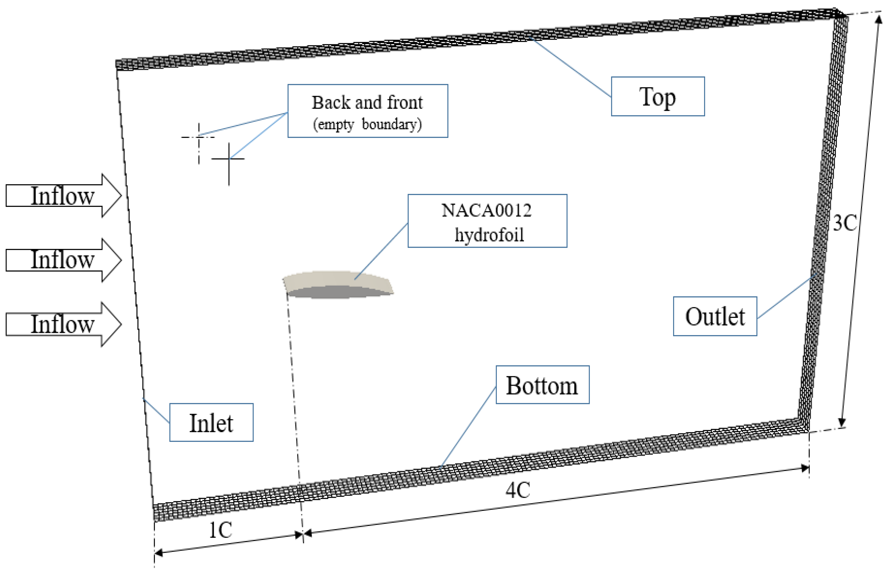
3.1. Two-Dimensional Computational Domain and Boundary Condition
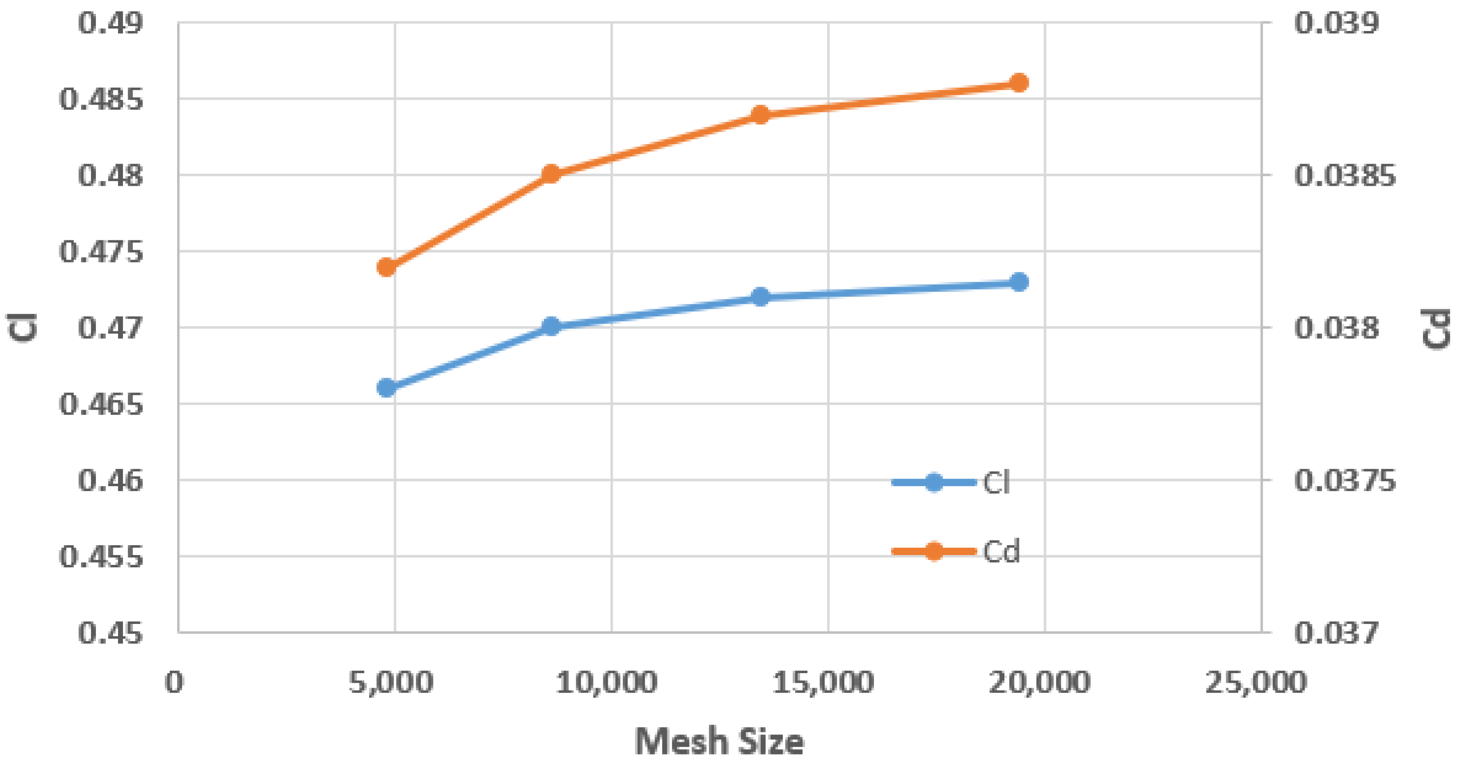
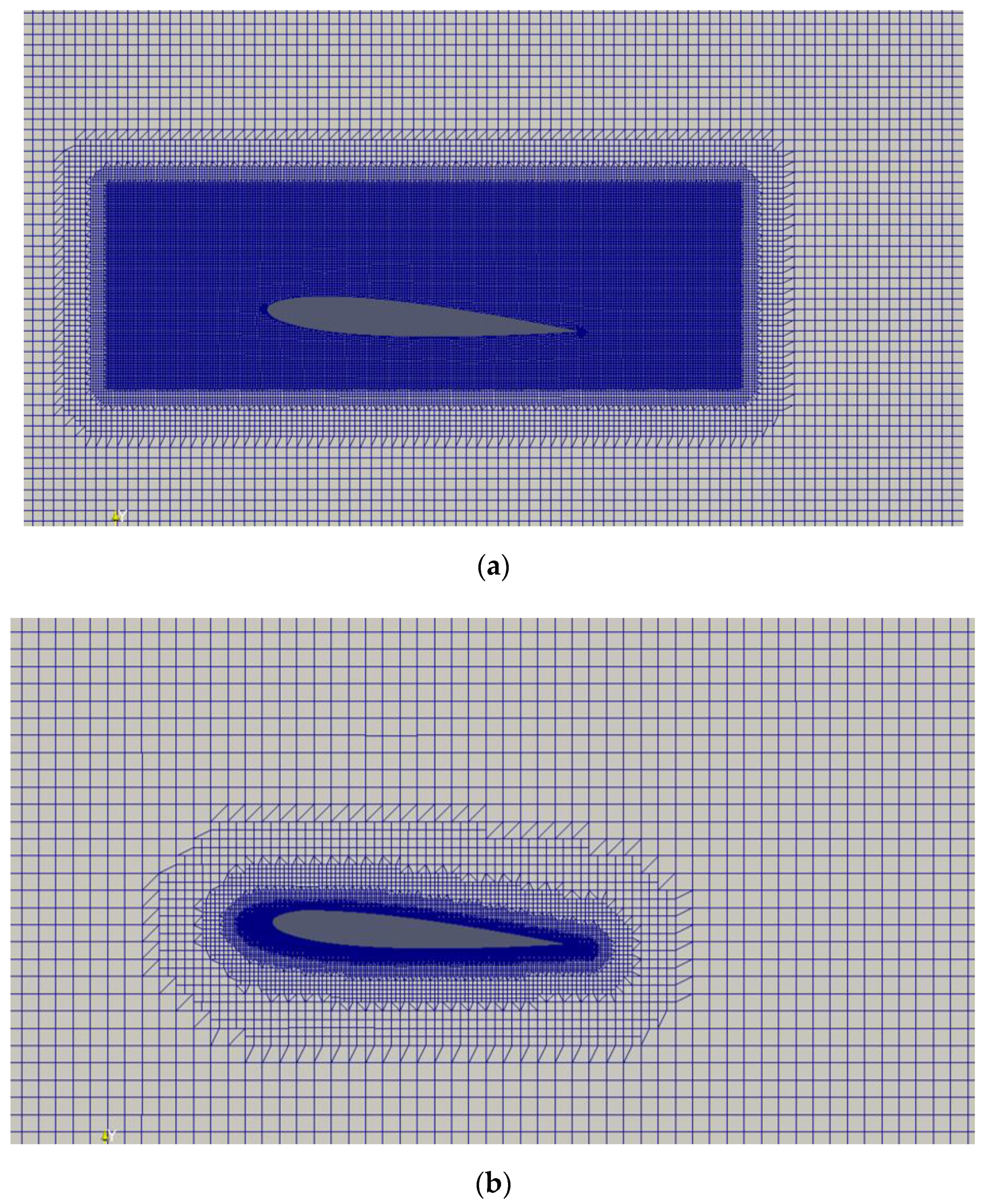
For the investigations in the computational domain, the test geometry is a NACA0012 hydrofoil at an angle of attack of 4 degree with the chord length C = 100 mm. The computational domain is shown in Figure 1. The size of the domain is 500 × 300 mm. All distances in the section were based on the chord length C. The span-wise domain width is 0.277 mm. The inlet of the computational domain is 1C upstream from the leading edge and 4C downstream from the leading edge for the outlet of the computational domain; other detailed boundary conditions are described in Table 1 with nonslip condition for the wall. The first-order Euler scheme was used for temporal discretization, and the first-order upwind scheme was used for spatial discretization; the near-wall region was solved directly. In the simulation, the first-order discretization was chosen to reduce the calculation time, but it has disadvantages in accuracy; therefore, a second order discretization is recommended.
The inlet velocity was 5 m/s, and the pressure gradient at the outlet was zero. Reference pressure was calculated by the cavitation number through Equation (13). The cavitation number in the present work is 0.8. The viscosity and density of liquid in the flow field are the same as those of water at room temperature. The parameters of the work condition are listed in Table 2. As for the usage of PIMPLE coupling, the number of iteration is 2.
σ = P P v 1 2 ρ U 2

3.2. Mesh Size

The influence of the mesh size was considered in the present paper. To find out the appropriate mesh size for the numerical simulation setup, three kinds of mesh were calculated and analyzed. Specific grid information and corresponding calculation results are listed in Table 3. The mesh dependency of the lift and drag coefficients are shown in Figure 2. It was found that the force coefficients increased clearly when the mesh number was small, and the difference decreased fast when the mesh became fine. A verification and validation of lift coefficient was calculated, and the results are shown in Table 3. The lift coefficient in the experimental data is 0.52. The experimental uncertainty is 1%. The value of calculated numerical uncertainty is 0.00658. From the verification and validation results, it can be seen that the value of numerical uncertainty is larger than the comparison error. Therefore, the convergence of the calculated results exists, but the certainty of the results is not confirmed. The values of y+, z+ and x+, are about 1, 20 and 50, respectively.

3.3. Computational Domain

During mesh generation, a region-wide background grid was established first. Then, we used the snappyHexMesh method in the OpenFOAM platform for mesh refinement. This process is meant for better capturing the force on the NACA0012 two-dimensional hydrofoil and the cavitation on the back side of the blade.
The sketch map of the grids in the computational domain is shown in Figure 3. The mesh system has three parts. The first part is the outer mesh, which is the initial mesh for the whole flow field; from Figure 3a, we can see the second part, whose length is twice as the length of the chord length, and the height is 2D. Figure 3a is the refinement mesh, which has a three-level refinement based on the initial mesh in the entire computational domain grid for the simulation using the SST k-ω turbulence model and the modified SST k-ω turbulence model with a mesh size of 595,603 cells. In the simulation using the Smagorinsky turbulence model, the refinement mesh is different, and it is shown in Figure 3b. As can be seen, this kind of structural grids requires a larger level of refinement than the others. The mesh refinement method is a relatively better approach for generating the grids. The size number of the cells is 3,705,390.
The computation duration was 2 s long to ensure that the cavitation flow is fully developed and the shedding frequency can be obtained. The computational time step needs to be small enough to avoid the numerical divergence that happens in time and so that more accurate numerical data could be obtained. The time step was 0.0004 s with the SST k-ω turbulence model, and 0.00005 s with the Smagorinsky turbulence model. It should be noted that the cavitation number also has a strong influence on the simulation results; in the present study, this part is not investigated.

4. Result and Discussions

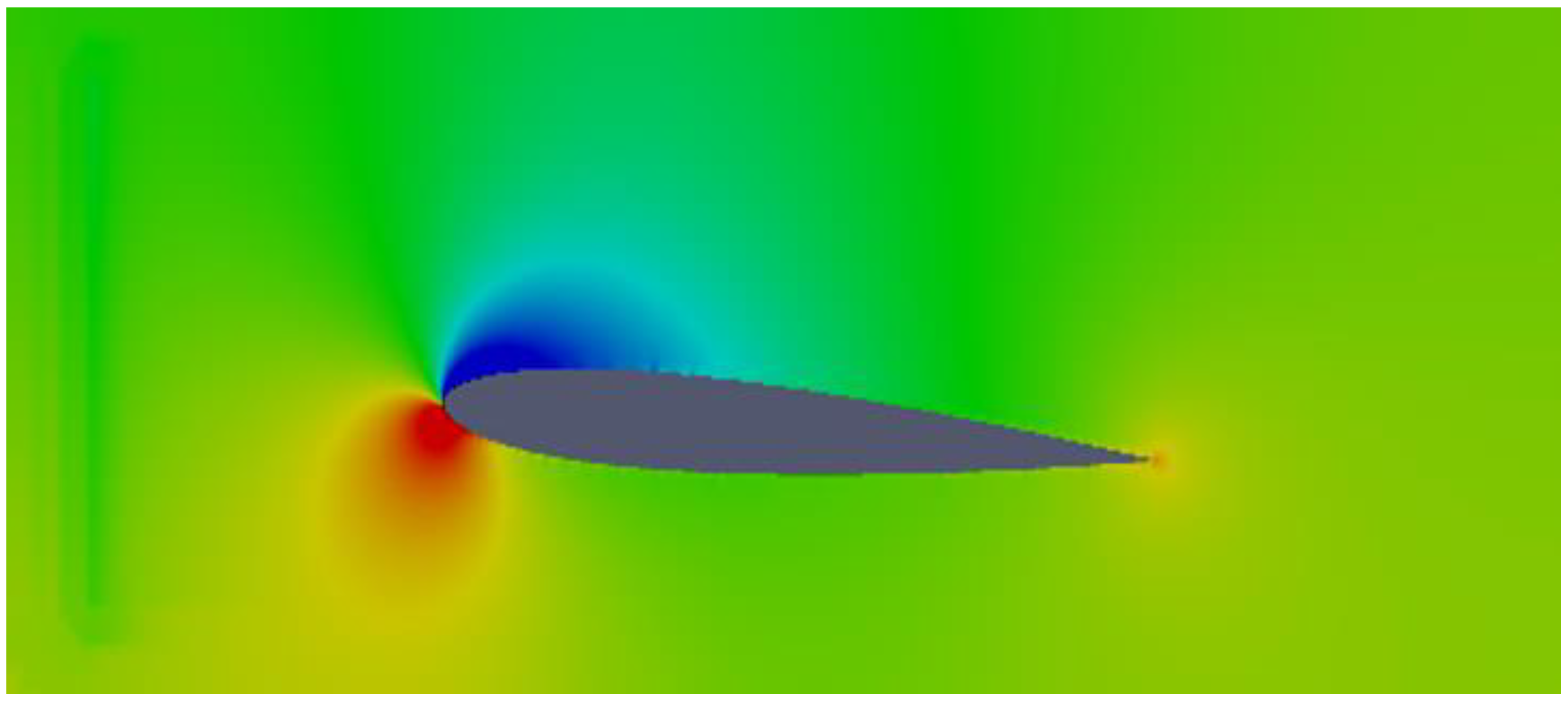
4.1. Cavitation Flow

Firstly, the non-cavitating steady flow was calculated to verify the performance of the grid and the simulated pressure at a 4-degree angle of attack. As can be seen from Figure 4, when the flow is separated, there is a low-pressure area on the suction side of the NACA0012 hydrofoil and a high-pressure area on the pressure side. There is also a local high-pressure region at the tail of the hydrofoil. This phenomenon was simulated in the non-cavitating steady flow. The pressure coefficient distribution is also shown in Figure 5.
The simulated pressure distribution was consistent with the results calculated by Adjali et al. [30]. The values of tail high pressure point, the low pressure point, and the slightly high pressure point were also consistent with those of Adjali et al. [30]. The results show that the detailed information of the flow field from the NACA0012 wet flow simulation results calculated by OpenFOAM is reliable.
The pressure coefficients between the cavitation flow field and the non-cavitation flow field in steady condition were compared, as shown in Figure 6. In the cavitation flow, the pressure in the cavitation zone was equal to the vapor pressure. The pressure distribution on the suction side of the membrane was greatly affected by the cavitation effect, and the pressure gradient at the closure of the membrane cavity was much larger than that at the same location under the non-cavitation flow. However, the change on the pressure side of the foil was much smaller. The change of pressure distribution also led to significant changes in the overall hydrodynamic performance of the hydrofoil. In the calculation of initial non-cavitating flow, the lift and drag forces acting on hydrofoil are cl = 0.489 and cd = 0.0361, which were larger and smaller than those calculated under cavitating flow, i.e., cl = 0.472 and cd = 0.0387, respectively. The results show that the local cavitation of the leading edge of the hydrofoil can inhibit the lift and enhance the drag.
The two-dimensional cloud cavitation phenomena of NACA0012 hydrofoil in a uniform flow field at 4 and 8-degree of attack and under 0.8 cavitation numbers were studied and compared with the experimental results. The calculated cavitation shape and vapor content were shown in Figure 7 and Figure 8. In Figure 7, the angle of attack of the two-dimensional hydrofoil is 4 degrees, and in Figure 8, the angle of attack is 8 degrees. The numerical results of three different turbulence models are given. It can be seen that the cavitation flow was unsteady. Different stages of cavitation, such as growth and collapse, were simulated.

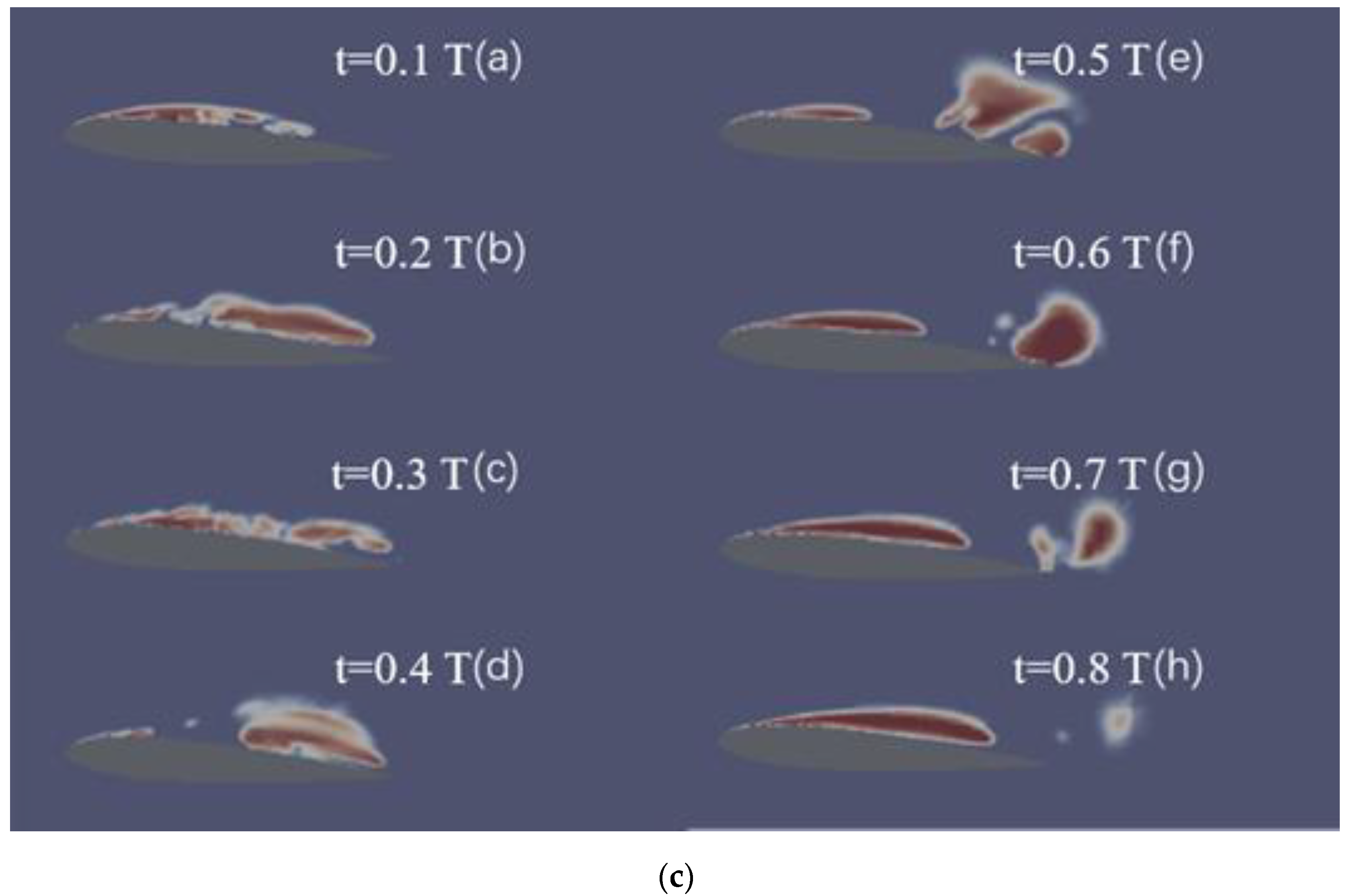
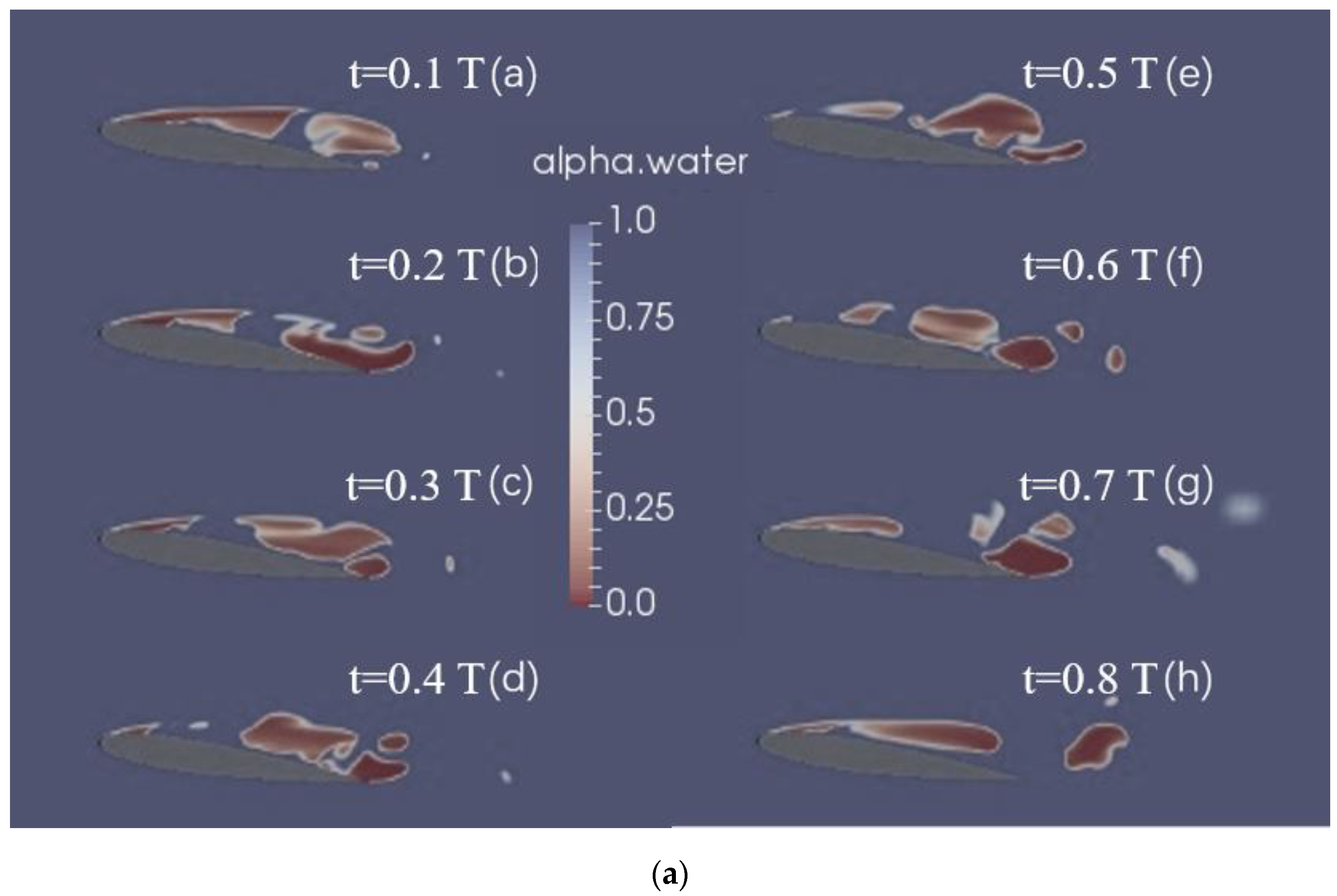
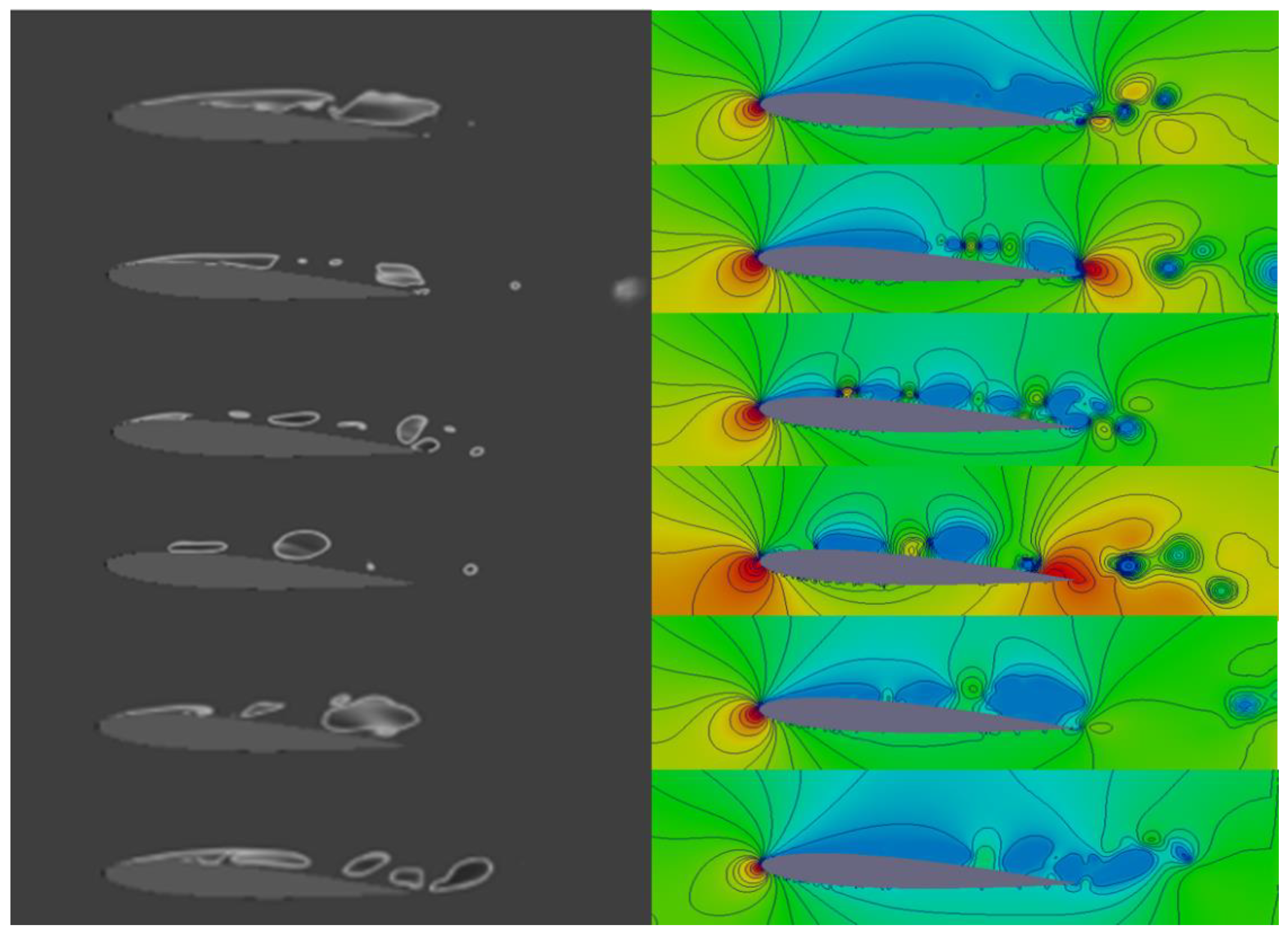
4.2. Unsteady Cavitation at 4-Degree Angle of Attack

In the whole process of cavitation development, the simulation of NACA0012 cavitation process using Smagorinsky’s turbulence model has obvious an advantage in capturing the small vortices structures. In Figure 7, it can be seen that the voids consisting of tiny voids and droplets of small thickness were generated at the head of the hydrofoil firstly. At that time, the cavity was still attached to the surface of the hydrofoil. As time goes on, the attached cavity continued to develop towards the tail of the hydrofoil. The thickness of the cavity increased along the wing chord and reached its maximum gradually. The end of the cavity was located at the tail of the hydrofoil. Meanwhile, the small vortices fell off at the end of the cavity. Then, the cavity was divided into two parts. The front part was attached to the suction surface of the hydrofoil, and the tail part of the cavity fell off and moved downstream.
Smagorinsky’s turbulence model can be used to simulate large-scale fluctuations. We observed that obvious unsteady cavitation vortices were captured by this model. On the other hand, the SST k-ω model is a kind of RANS model, which treats vortices of different scales equally. Therefore, the prediction ability of separated flow of this model is rather poor. The vorticity structure captured by Smagorinsky model is more abundant than that captured by the SST k-ω model because of the way it treats the vortices. The modified SST k-ω model artificially reduces the turbulent viscosity to suppress the effect of excessive viscosity. In Figure 7, the cavitation breakdown and shedding phenomena changed more obviously with time, and the small vortices captured were more abundant than those captured by the modified SST k-ω model. Smagorinsky’s model in OpenFOAM is a static Smagorinsky model, which has some disadvantages in dealing with wall problems; however, the main research of this paper in cavitation simulation is focused on the tail and above of hydrofoil. It is recommended to use the dynamic Smagorinsky model in the simulation, which uses the quadratic filtering function to obtain better results near the wall.
Previous studies have shown that when the cavitation number decreases or the angle of attack increases, the cavitation flow becomes more unsteady, which means that the unsteady characteristics cavitation flow are relatively smooth at small angle of attack. Although the LES method can provide more detailed cavitation flow field, the Smagorinsky turbulence model also needs more computation work. On the other hand, the modified SST k-ω turbulence model simulates unsteady cavitation well compared with the SST k-ω turbulence model, and the computational cost is relatively small. Therefore, the modified SST k-ω turbulence model is more satisfactory than SST k-ω turbulence model and is more practical than the Smagorinsky model at small angles of attack.

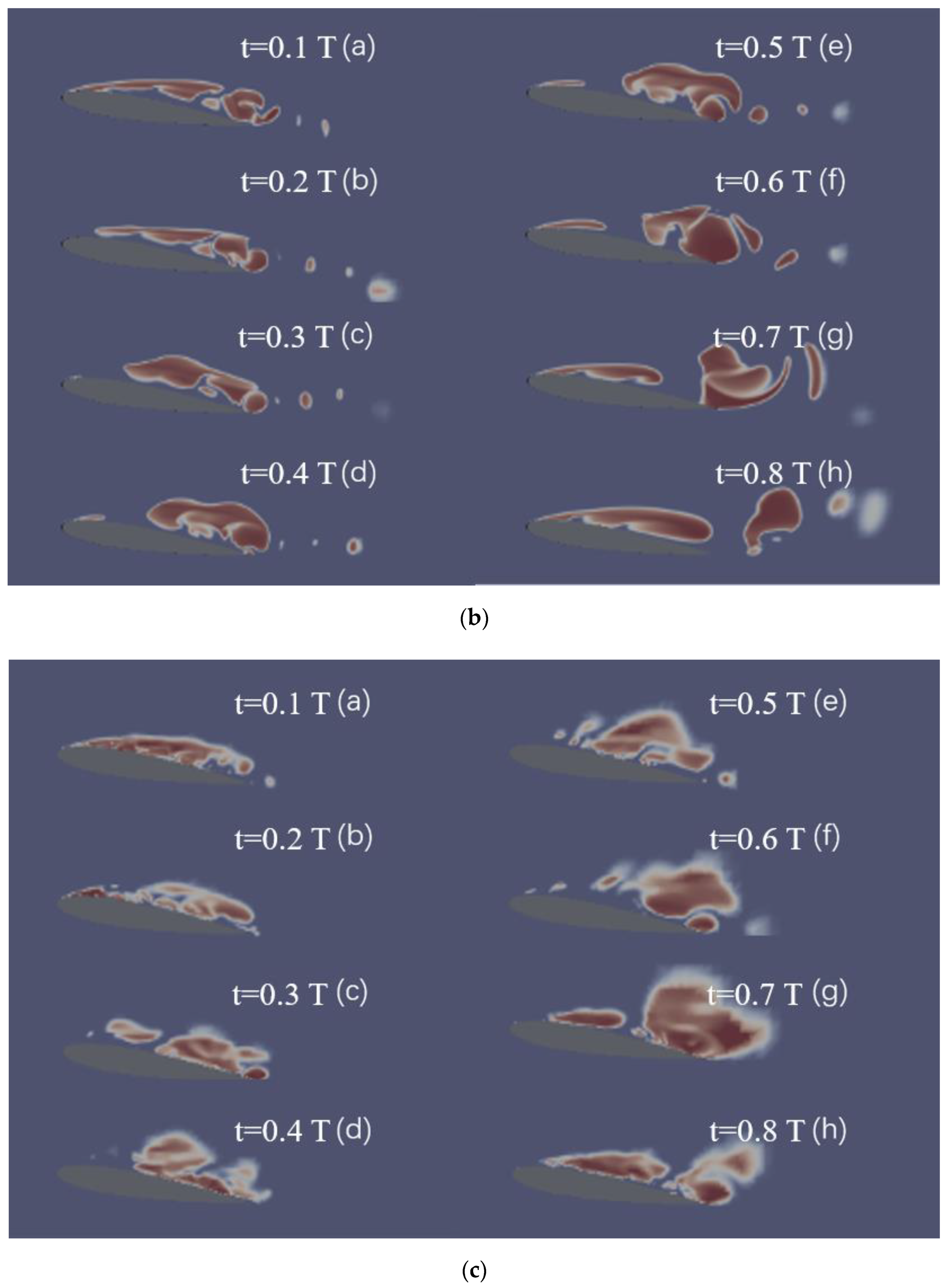
4.3. Unsteady Cavitation at 8-Degree Angle of Attack

The simulation results of cavitating the flow of the NACA0012 hydrofoil at 8 degrees of attack are shown in Figure 8. Obviously, when the angle of attack was 8 degrees instead of 4 degrees, the cavitation was more unsteady. In the cloud cavitation around the hydrofoil, the wake and separated vortices at the tail of the hydrofoil were very obvious. Compared with the SST k-ω model, the maximum length of cavity calculated by Smagorinsky’s model decreased at a slower rate. In the cavitation vortex shedding stage, the Smagorinsky model can more accurately capture the water-vapor mixing structure at the tail of the hydrofoil, which is consistent with the experimental results [31].
In the early stage of this period, a sheet cavity with fairly pure vapor appeared at the front of the hydrofoil and it started to move downstream. In the last stage, cloud cavitation occurred in the wake, and collapses occurred when the cavity reached about 1/3 of the chord length. Because of the unbalanced flow field and the development of the low-pressure zone, the sheet cavity was further expanded. At the same time, when the cavity increased to a certain extent, the pressure at the closure of the sheet cavity increased, resulting in a re-entrant jet pointing to the leading edge.
In addition, the Smagorinsky model captured the unsteady details of void mass shedding in time-dependent vortices in a better way. According to the numerical results of SST k-ω, there was only one cavitation group at the end of the hydrofoil, which was different from the experimental observations [31]. Objectively speaking, compared with SST k-ω turbulence model, the modified SST k-ω turbulence model still has advantages in simulating sheet cavitation around the NACA0012 hydrofoil. However, for the modified SST k-ω turbulence model, the unsteady cavitation flow field was too complex to capture. The disadvantage of the RANS method in dealing with unsteady details cannot be compensated easily. Therefore, the Smagorinsky model based on the LES method is more suitable for cavitation simulation at a large angle of attack.
Figure 9 shows the contours of a series of instantaneous vapor distributions and pressure coefficients over a period of time. In the figure, the area covered by cloud cavitation represents the place where the local pressure drops below the vapor pressure. The maximum length and thickness of the cavity are much larger than the steady sheet cavity.

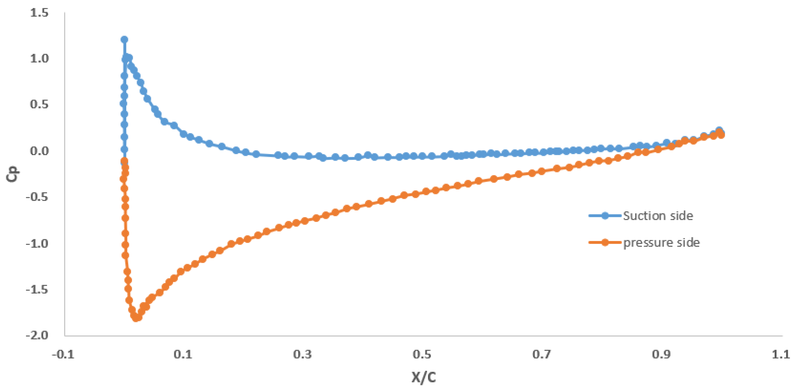
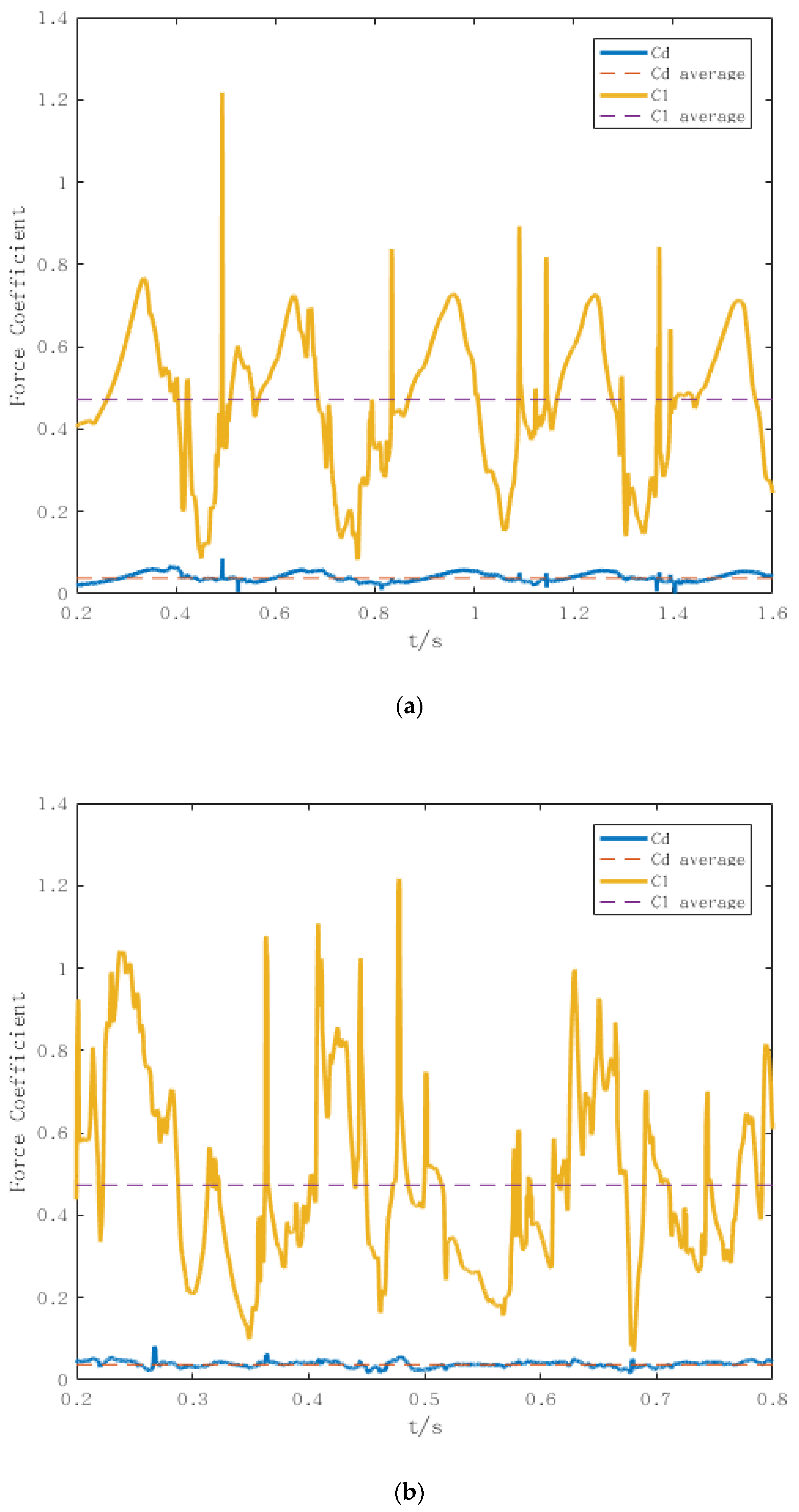
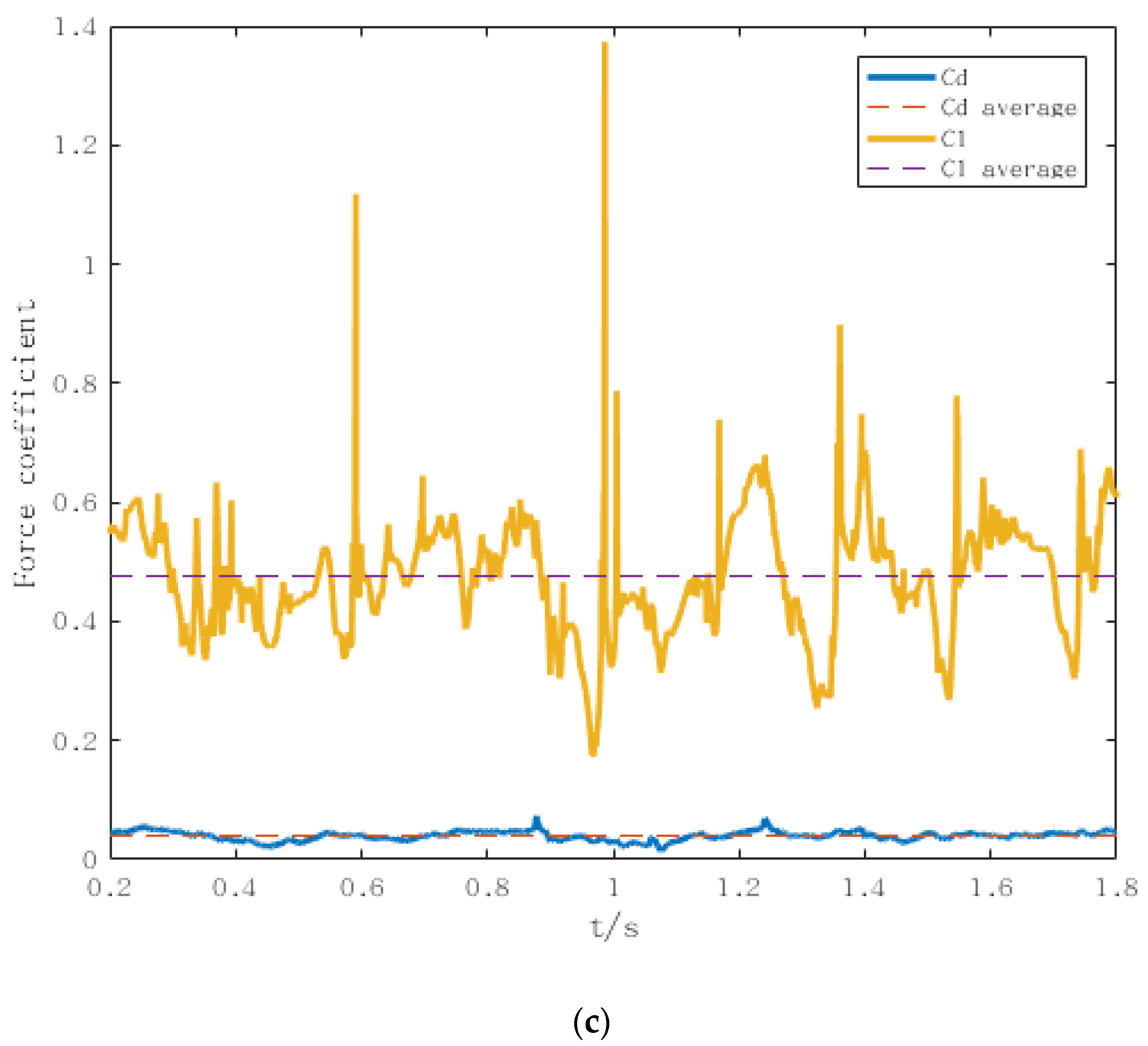
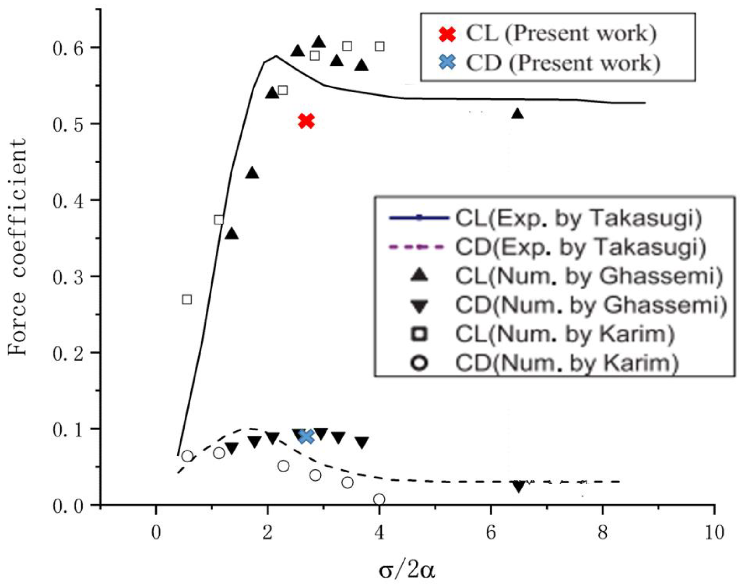
4.4. Hydrodynamic Characteristics

The curves of lift–drag coefficients with time of two-dimensional hydrofoils calculated by three different turbulence models are shown in Figure 10. It can be seen from the figure that the shedding frequencies of the three models are obviously different. The frequency calculated by the SST k-ω turbulence model is 4.098 Hz. The frequency calculated by the modified SST k-ω turbulence model is 6.410 Hz. The calculated frequency of the Smagorinsky turbulence model is 5.405 Hz.
Compared with the other two models, the results simulated by the SST k-ω model are fairly smooth. This is consistent with the phenomenon in Figure 8. The SST k-ω turbulence model has poor ability to simulate the generation and a decline of small cavitation, and it is difficult to see the continuous small cavitation falling off during the whole process. Therefore, the influence of small cavitation on lift coefficient fluctuation cannot be well reflected.
The results of the modified SST k-ω turbulence model in Figure 10b show that the small vortices keep falling off. The effect of reducing turbulent viscosity artificially was remarkable, but on the other hand, the periodicity was affected. In Figure 10a, the periodic fluctuation characteristics of the time-history curve are obvious, and in Figure 10b, the periodic variation characteristics are concealed by the curve fluctuation to some extent.
In Figure 10c, the fluctuation of the lift–drag coefficient of the two-dimensional hydrofoil calculated by Smagorinsky’s model is the most obvious. This is because the LES method can capture unsteady vortices, and the details of cavitation flow field are abundant, as shown in Figure 7. Compared with the work of other researchers, the lift and drag coefficients are relatively accurate. The results are listed in Table 4.
The comparison of the experimental results with those of other numerical results and the present work using the modified SST k-ω model is shown in Figure 11. In the present work, the calculated values of the lift and drag coefficients are respectively smaller and larger than those of the experimental data.

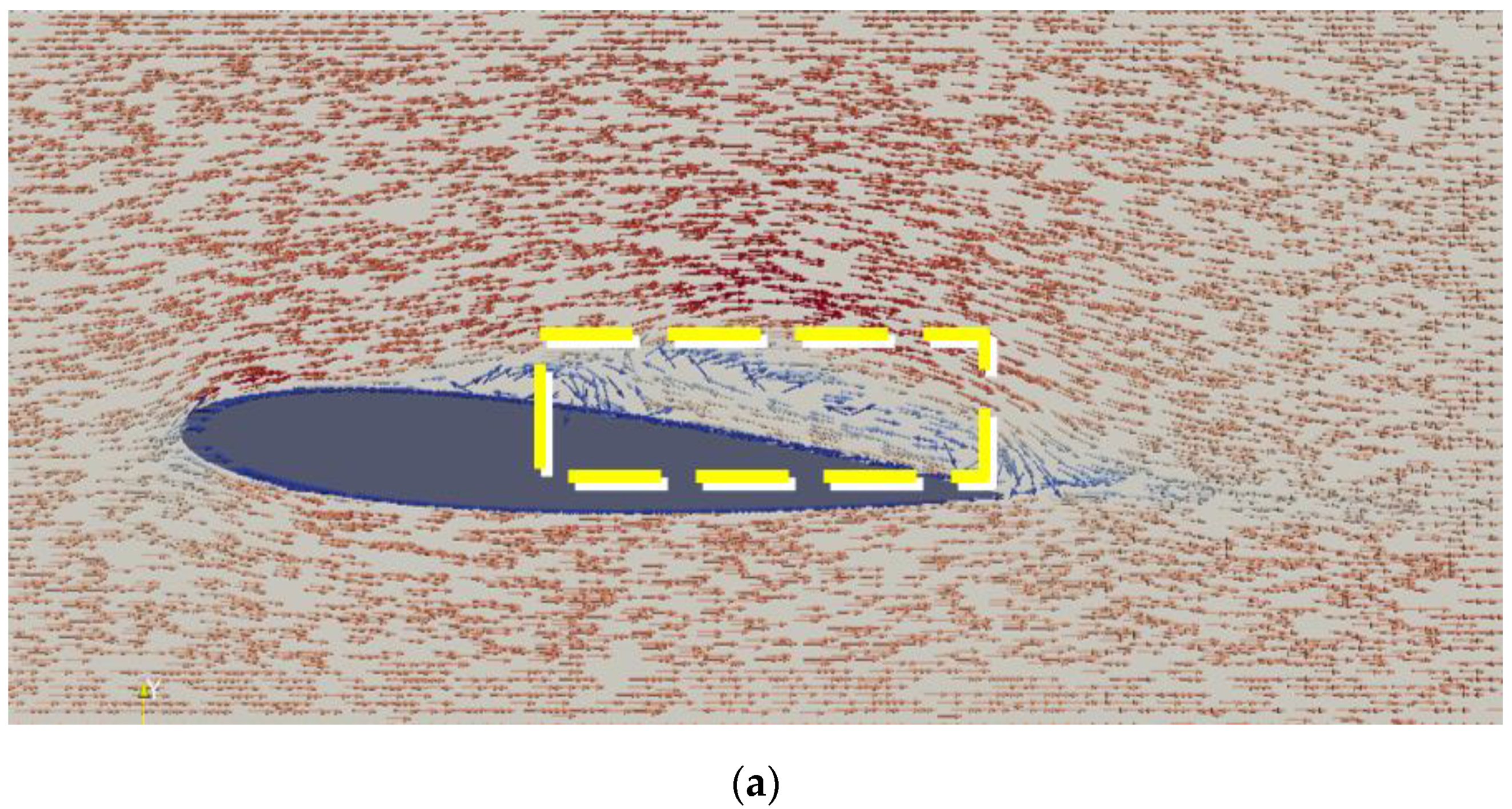
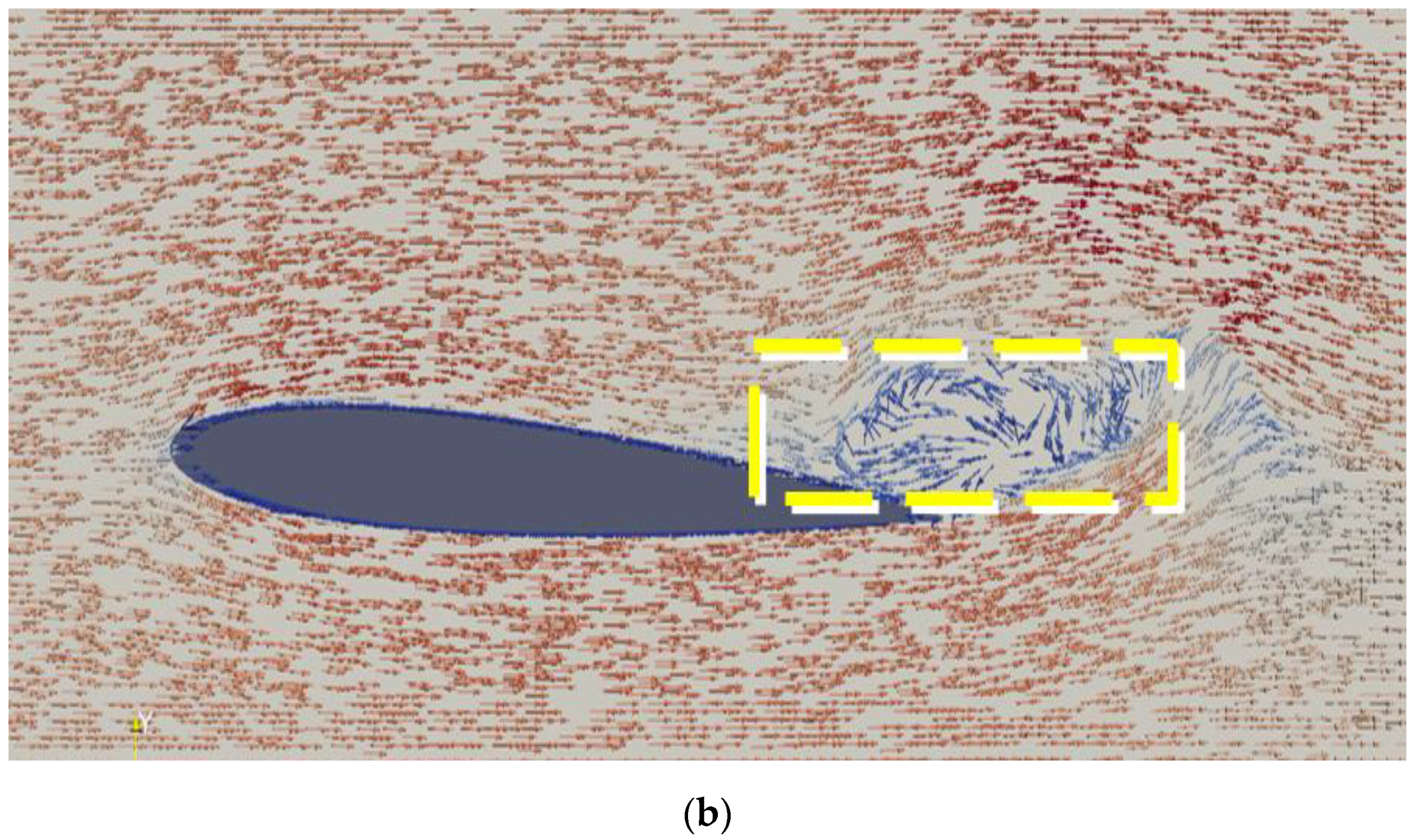
4.5. Analysis about the Mechanism of Periodical Change in Cavitation

The retraction at the junction part between the end of the inner cavity and the hydrofoil shows that there was a re-entrant jet, which caused the small bubbles falling off at the end of the cavity. In Figure 7a(d–g),b(d–g),c(d–g), the incoming flow flowed to the middle part of the hydrofoil, leading to an unsteady cloud cavitation, which moved downward along the hydrofoil to form distinct cloud droplets in the progress. The numerical results generally captured the fracture and detachment behaviors in the process of cavitation and were in good agreement with the experimental observation.
The velocity vector picture during cavitation is shown in Figure 12. Both the re-entrant jet in the region between the cavitation and wall, and the vortex structure that occurs at the tail during the growth of sheet cavitation were accurately predicted by analyzing the velocity vector diagram. The vortex structure caused the re-entrant jet to appear, which led to the cloud cavitation because of the sheering action during the collision. Hence the vortex is actually the reason for cavitation shedding in the process.
To sum up, three turbulence models, the SST k-omega model, Smagorinsky’s turbulence model, and the modified SST k-omega model, were used. The results of shedding frequencies of these three turbulence models in all cases obtained from the data of the calculation output and the observation of the cavitation shedding are shown in Table 5, and these were compared with the data of other authors. The results show that the modified SST k-omega model can predict the shedding frequency well when the n value is 10. The frequency value predicted by Smagorinsky’s model is also slightly larger, while the performance of SST k-omega model is not good.
In addition, compared with Figure 7 and Figure 8, Smagorinsky’s model and the modified SST k-omega model performed better than the SST k-omega model in the modeling of cavitation shape in the process of periodic change, especially during cavitation shedding. In the corresponding diagrams of the Smagorinsky and the modified SST k-omega model, we can clearly observe the multiple shedding of sheet cavitation, not only once or twice, but also the simultaneous existence of multiple cloud bubbles in different regions of the suction side, although the same phenomenon cannot be observed in Figure 7.

5. Conclusions

In this paper, three different turbulence models were used to simulate the cloud cavitation around the NACA0012 hydrofoil using the interPhaseChangeFoam solver in OpenFOAM. The hydrodynamic characteristics and cavitation flow were demonstrated and compared with each other, and the following conclusions can be drawn:
(a)
Generally speaking, the modified SST k-ω model and the Smagorinsky model are better than the SST k-ω model in simulating unsteady cavitation flow.
(b)
In the case of a small angle of attack, the modified SST k-ω model is more accurate and practical than the SST k-ω model, and the calculation cost is lower than Smagorinsky’s model.
(c)
At a large angle of attack, the cavitation around the hydrofoil becomes more unsteady, and the two SST k-ω models based on the RANS method cannot accurately capture the details of the vortices in the flow field. The simulation results of Smagorinsky model based on LES method are in good agreement with the experimental results.
(d)
The numerical results generally capture the fracture and detachment behaviors in the process of cavitation and are in good agreement with the experimental observation. Further research on re-entrant jet shows that the vortex structure at the tail of hydrofoil is the main reason for cavitation shedding.

Author Contributions

M.Z. is responsible for document retrieval, numerical simulation and manuscript writing; D.W. is responsible for research and design, data analysis and manuscript verification; Y.G. is responsible auxiliary analysis. All authors have read and agreed to the published version of the manuscript.

Funding

National Key Research and Development Program of China (2019YFB1704200 and 2019YFC0312400) and the National Natural Science Foundation.

Institutional Review Board Statement

Not applicable.

Informed Consent Statement

Not applicable.

Data Availability Statement

Not applicable.

Acknowledgments

This work is supported by the National Key Research and Development Program of China (2019YFB1704200 and 2019YFC0312400) and the National Natural Science Foundation of China (51879159), to which the authors are most grateful.

Conflicts of Interest

The authors declare no conflict of interest.

References

  1. Crimi, P. Experimental study of the effects of sweep on hydrofoil loading and cavitation. J. Hydraul. 1970, 4, 3–9. [Google Scholar]
  2. Bark, G. Development of violent collapses in propeller cavitation. In International Symposium on Cavitation and Multiphase Flow Noise; ASME-FED: Anaheim, CA, USA, 1986; Volume 45, pp. 65–75. [Google Scholar]
  3. Dular, M.; Bachert, R.; Schaad, C.; Stoffel, B. Investigation of a re-entrant jet reflection at an inclined cavity closure line. Eur. J. Mech. B-Fluids 2007, 26, 688–705. [Google Scholar] [CrossRef]
  4. De Lange, D.F.; De Bruin, G.J. Sheet cavitation and cloud cavitation, re-entrant jet and three-dimensionality. Appl. Sci. Res. 1998, 58, 91–114. [Google Scholar] [CrossRef]
  5. Katz, J. Cavitation phenomena within regions of flow separation. J. Fluid Mech. 2006, 140, 397–436. [Google Scholar] [CrossRef] [Green Version]
  6. Hackworth, J.V. Predicting Cavitation Erosion of Ship Propellers from the Results of Model Experiments. In Proceedings of the Fifth International Conference on Erosion by Liquid and Solid Impact, Cambridge, UK, 3–6 September 1979. [Google Scholar]
  7. Hackworth, J.V.; Arndt, R.E.A. Preliminary Investigation of the Scale Effects of Cavitation Erosion in a Flowing Media. In Cavitation and Polyphase Flow Forum; ASME: Anaheim, CA, USA, 1974. [Google Scholar]
  8. De Lange, D.F.; De Bruin, G.J.; Van Winjngaarden, L. On the mechanism of cloud cavitation: Experiment and modeling. In Proceedings of the Second International Symposium on Cavitation, Tokyo, Japan, 5–7 April 1994. [Google Scholar]
  9. Karabelas, S.J.; Markatos, N.C. Water vapor condensation in forced convection flow over an airfoil. Aerosp. Sci. Technol. 2008, 12, 150–158. [Google Scholar]
  10. Timoshevskiy, M.V.; Ilyushin, B.B.; Pervunin, K.S. Statistical structure of the velocity field in cavitating flow around a 2D hydrofoil. Int. J. Heat Fluid Flow 2020, 85, 108646. [Google Scholar] [CrossRef]
  11. Zhang, M.; Huang, B.; Wu, Q.; Zhang, M.; Wang, G. The interaction between the transient cavitating flow and hydrodynamic performance around a pitching hydrofoil. Renew. Energy 2020, 161, 1276–1291. [Google Scholar] [CrossRef]
  12. Huang, B.; Qiu, S.C.; Li, X.B.; Wu, Q.; Wang, G.Y. A review of transient flow structure and unsteady mechanism of cavitating flow. J. Hydrodyn. 2019, 31, 429–444. [Google Scholar] [CrossRef]
  13. Huang, R.F.; Du, T.Z.; Wang, Y.W.; Huang, C.G. Numerical investigations of the transient cavitating vortical flow structures over a flexible NACA66 hydrofoil. J. Hydrodyn. 2020, 32, 234–246. [Google Scholar] [CrossRef]
  14. Chen, Y.; Li, J.; Gong, Z.; Chen, X.; Lu, C. Large Eddy Simulation and investigation on the laminar-turbulent transition and turbulence-cavitation interaction in the cavitating flow around hydrofoil. Int. J. Multiph. Flow 2019, 112, 300–322. [Google Scholar] [CrossRef]
  15. Liang, S.; Li, Y.; Wan, D.C. Numerical simulation of cavitation around Clark-Y hydrofoil based on adaptive mesh refinement. Chin. J. Hydrodyn. 2020, 35, 1–8. [Google Scholar]
  16. Wang, Z.; Huang, X.; Cheng, H.; Ji, B. Some notes on numerical simulation of the turbulent cavitating flow with a dynamic cubic nonlinear sub-grid scale model in OpenFOAM. J. Hydrodyn. 2020, 32, 790–794. [Google Scholar] [CrossRef]
  17. Merkle, C.L.; Feng, J.Z.; Buelow, P.E.O. Computational modeling of the dynamics of sheet cavitation. In Proceedings of the 3rd International Symposium on Cavitation, Grenoble, France, 7–10 April 1998. [Google Scholar]
  18. Kunz, R.F.; Boger, D.A.; Stinebring, D.R.A. Preconditioned Navier-Stokes method for two-phase flows with application to cavitation prediction. Comput. Fluids 2000, 29, 849–875. [Google Scholar] [CrossRef]
  19. Yuan, W.; Sauer, J.; Schnerr, G.H. Modeling and computation of unsteady cavitation flows in injection nozzles. MEC Ind. 2001, 2, 383–394. [Google Scholar] [CrossRef]
  20. Singhal, A.K.; Li, N.H.; Athavale, M.; Li, H.; Jiang, Y. Mathematical basis and validation of the full cavitation model. J. Fluids Eng. 2002, 143, 617–624. [Google Scholar] [CrossRef]
  21. Huang, B.; Wang, G.Y.; Zhao, Y.; Wu, Q. Physical and numerical investigation on transient cavitating flows. Sci. China Technol. Sci. 2013, 56, 2207–2218. [Google Scholar] [CrossRef]
  22. Li, Z.; Mathieu, P.; van Terwisga, T. Assessment of Cavitation Erosion with a URANS Method. J. Fluids Eng. 2014, 136, 041101. [Google Scholar] [CrossRef]
  23. Zhang, L.X.; Chen, M.; Deng, J.; Shao, X.M. Experimental and numerical studies on the cavitation over flat hydrofoils with and without obstacle. J. Hydrodyn. 2019, 31, 708–716. [Google Scholar] [CrossRef]
  24. Wang, Y.Q.; Yu, H.D.; Zhao, W.W.; Wan, D.C. Liutex-based vortex control with implications for cavitation suppression. J. Hydrodyn. 2021, 33, 74–85. [Google Scholar] [CrossRef]
  25. Zhao, M.S.; Zhao, W.W.; Wan, D.C. Numerical simulations of propeller cavitation flows based on OpenFOAM. J. Hydrodyn. 2020, 32, 1071–1079. [Google Scholar] [CrossRef]
  26. Zhang, X.S.; Wang, J.H.; Wan, D.C. An improved multi-scale two phase method for bubbly flows. Int. J. Multiph. Flow 2020, 133, 103460. [Google Scholar] [CrossRef]
  27. Schnerr, G.H.; Sauer, J. Physical and numerical modeling of unsteady cavitation dynamics. In Proceedings of the 4th International Conference on Multiphase Flow, New Orleans, LA, USA, 27 May 2001. [Google Scholar]
  28. Reboud, J.L.; Stutz, B.; Coutier-Delgosha, O. Two Phase FlowStructure of Cavitation Experiment and Modeling of Unsteady Effects. In Proceedings of the 3rd International Symposium, Cavitation, Grenoble, France, 13–15 August 1998. [Google Scholar]
  29. Menter, F.R. Two-equation eddy-viscosity turbulence models for engineering applications. AIAA J. 1994, 32, 1598–1605. [Google Scholar] [CrossRef] [Green Version]
  30. Adjali, S.; Belkadi, M.; Aounallah, M.; Imine, O. A numerical study of steady 2D flow around NACA 0015 and NACA 0012 hydrofoil with free surface using VOF method. EPJ Web Conf. 2015, 92, 02001. [Google Scholar] [CrossRef] [Green Version]
  31. Wang, G.; Senocak, I.; Shyy, W.; Ikohagi, T.; Cao, S. Dynamics of attached turbulent cavitating flows. Prog. Aerosp. Sci. 2001, 37, 551–581. [Google Scholar] [CrossRef]
Figure 1. The grid in the lengthwise section and the cross section.
Jmse 09 00742 g001
Figure 2. Lift and drag coefficient variations along with the mesh resolution.
Jmse 09 00742 g002
Figure 3. Computational mesh around NACA0012 hydrofoil. (a) Mesh with SST k-ω turbulence model. (b) Mesh with Smagorinsky turbulence model.
Jmse 09 00742 g003
Figure 4. Pressure distribution of the flow fields.
Jmse 09 00742 g004
Figure 5. Pressure coefficient on the surface of NACA0012 in the present paper.
Jmse 09 00742 g005
Figure 6. Contrast between the pressure distributions of the cavitating and non-cavitating flows. (a) Pressure distributions of the cavitating flows. (b) Pressure distributions of the non-cavitating flows.
Jmse 09 00742 g006
Figure 7. Change of cavitation morphology with different turbulence models at a 4-degree angle of attack. (a) Simulation of cavitation with SST k-ω turbulence model. (b) Simulation of cavitation with modified SST k-ω turbulence model. (c) Simulation of cavitation with the Smagorinsky turbulence model.
Jmse 09 00742 g007aJmse 09 00742 g007b
Figure 8. Change of cavitation morphology with different turbulence models at an 8-degree angle of attack. (a) Simulation of cavitation with SST k-ω turbulence model. (b) Simulation of cavitation with modified SST k-ω turbulence model. (c) Simulation of cavitation with the Smagorinsky turbulence model.
Jmse 09 00742 g008aJmse 09 00742 g008b
Figure 9. Evolution of the periodic sheet/cloud cavitating flow (contours of vapor fraction and pressure coefficient).
Jmse 09 00742 g009
Figure 10. Variation of lift and drag coefficient with time. (a) SST k-ω turbulence model. (b) Modified SST k-ω turbulence model. (c) Smagorinsky’s turbulence model.
Jmse 09 00742 g010aJmse 09 00742 g010b
Figure 11. Comparison of the mean lift and drag with experimental and other numerical results.
Jmse 09 00742 g011
Figure 12. Velocity vector of the flow fields. (a) Re-entrant jet. (b) Vortex structure.
Jmse 09 00742 g012aJmse 09 00742 g012b
Table 1. Boundary conditions.
HydrofoilWall
InletVelocity
OutletPressure
Top and BottomWall
Front and backSymmetry
Table 2. Parameters of work condition.
Velocity5 m/s
Cavitation number0.8
K0.0185
Omega621.626
Pressure9358.6848
Chord length100 mm
Angle of attack4 degree and 8 degree
Table 3. Verification and validation of lift coefficient.
Parameter R G P C ( U V / D ) % ( U G C / D ) % ( U V C / D ) % ( E / D ) % ( E C / D ) %
Value0.68182.2101.1271.2650.078631.0039.2309.792
Table 4. Lift and drag coefficient in cavitation flow.
Lift CoefficientDrag Coefficient
Experiment results0.5200.035
SST k-ω model0.4720.0387
Modified SST k-ω model0.4730.0374
Smagorinsky model0.4760.0402
Table 5. Quantities predicted by the different turbulence models.
Frequency (Hz)
RANS, SST k-omega model
(special modified model when n = 1)
4.098
LES, Smagorinsky’s model5.415
RANS, modified SST k-omega model,6.410
Ying(2016)4.883
Publisher’s Note: MDPI stays neutral with regard to jurisdictional claims in published maps and institutional affiliations.

