
Development of Enhanced Two-Time-Scale Model for Simulation of Ship Maneuvering in Ocean Waves


Department of Naval Architecture and Ocean Engineering, Seoul National University, Seoul 08826, Korea
*
Author to whom correspondence should be addressed.
J. Mar. Sci. Eng. 2021, 9(7), 700; https://doi.org/10.3390/jmse9070700
Submission received: 30 May 2021
/
Revised: 14 June 2021
/
Accepted: 18 June 2021
/
Published: 25 June 2021
(This article belongs to the Special Issue Modelling and Optimisation of Ship’s Fuel Consumption for Realistic Operational Conditions)
Abstract
:In this study, a modified two-time-scale model is proposed to overcome the limitations of the existing maneuvering analysis model. To this end, not only wave conditions but also all directions of ship operation velocities are considered in estimating wave drift force and moment. Subsequently, the increment of the drift force and moment induced by steady drift and yaw motion of a ship is imposed up to the first derivative of Taylor series expansion. By introducing this bilinear model, the burden of the drift force computation is reduced so that a more realistic and efficient seakeeping-maneuvering coupling analysis can be performed. A turning circle simulation in a regular short wave is carried out using the modified two-time-scale model. Then, the performance is validated by comparing its results with the direct coupling model. Moreover, quantitative improvement of the present numerical scheme and the influence of the operation velocities on ship maneuvering performance are discussed.
1. Introduction
In general, a ship navigating in the real sea is affected by not only wave-making and frictional resistance but also by additional environmental load. This additional resistance degrades the operational performance of the ship, causes an increment of the required horsepower, and eventually leads to an increase in greenhouse gas emissions and environmental pollution. In particular, the added resistance induced by waves is known as the most prominent component that affects the operational performance of the ship. Therefore, accurate evaluation of the added resistance and mean drift forces induced by the waves have to be performed prior to the ship design in order to optimize the ship operational performance, eventually aiming for a reduction in fuel consumption and air pollution.
Recently, in accordance with international regulations on the minimum power capability of a ship operating in real environmental conditions, ship maneuverability in waves has become a primary interest in the fields of naval architecture and ship hydrodynamics. Since a reduction of the engine power for minimizing greenhouse gas emissions leads to deterioration of the ship stability and maneuvering performance, it is important to precisely assess ship maneuverability, especially in the adverse ocean environment [1,2]. However, evaluating ship maneuvering performance requires a sophisticated mathematical model and considerable simulation time, owing to its complexity. When a ship encounters a wave, its steering and propulsion performance is considerably affected. In addition, because a ship operating in waves experiences low-frequency maneuvering and high-frequency wave-induced motions simultaneously, the physical phenomena of both motions should be considered simultaneously. Therefore, many researchers have investigated reliable experimental and numerical techniques for estimating ship maneuverability in waves. In particular, international comparative research regarding various simulation models has been performed, e.g., the EU-funded Energy Efficient Safe SHip OPERAtion (SHOPERA, 2013–2016) project and a Japanese joint R&D project. According to these global research projects, additional studies should be performed to improve the capability of existing numerical tools [3]. In other words, the time efficiency and reliability of the maneuvering simulation model are still not mature.
Free-running experiments are the most reliable technique to analyze ship hydrodynamics, despite the significant time and cost incurred. To date, several researchers have conducted free-running experiments for various types of ships and have contributed to the validation of subsequent numerical studies. For instance, refs. [4,5,6] experimentally investigated the turning performance of the S175 container ship, ONR tumblehome, and the KVLCC2 tanker in regular incident waves, respectively. In addition, ref. [7] performed the free-running experiment for the KVLCC2 tanker, to evaluate maneuvering performance in irregular waves. In spite of its reliability, the free-running model test requires considerable time and cost to be performed practically. Moreover, existence of the scale effects and uncertainties are significant issues in the implementation of the model experiments. Hence, various numerical models have been developed to substitute model tests.
The two-time-scale model is the most widely adopted numerical model for evaluating ship maneuverability in waves owing to its simplicity. In this model, based on the assumption that the characteristic time scales of maneuvering and seakeeping problems are different, each physical quantity is separately calculated. To introduce seakeeping-maneuvering coupling effects, wave drift force and moment precomputed by the seakeeping analysis are imposed into maneuvering equations. Indeed, refs. [8,9,10] applied the two-time-scale model for investigating the maneuvering behavior of a ship in regular waves and showed that the incident waves can have a significant influence on the maneuvering performance of a ship. In addition, ref. [11] also carried out zig-zag and turning circle maneuver for two different types of ships in various regular wave conditions, by applying the two-time-scale model. Moreover, there was an effort to examine the capability of the abovementioned numerical model by comparing zig-zag maneuver in waves with the full-scale trial data [12]. In their numerical model, the main sources affecting the maneuvering performance of a ship are the wave drift force and moment. Inspired by these works, [13] investigated the contribution of each directional mean drift force by alternatively excluding them from the maneuvering equations of motion. Furthermore, ref. [14] extended earlier research of [8], by introducing their theoretical model to the irregular wave problem and using Newman’s approximation. They investigated the maneuvering behavior of a ship in various irregular wave conditions, i.e., significant wave height, mean wave periods, and random phase distribution, and found the influence.
Attributed to its simplicity, this model has a limitation that the memory effect cannot be taken into account, despite time-efficient maneuvering analysis being possible. Further, it is difficult to construct a wave drift force database in consideration of all components of ship operation velocities, thus only the influence of forward speed is reflected. However, according to the experimental studies conducted by [15,16], not only forward speed but also drift motion of a ship significantly affected the wave-induced mean drift force and moment. Inspired by these studies, ref. [17] applied the two-time-scale model for the problems of maneuvering in regular and irregular waves, additionally considering the influence of ship drift motion. Although the results showed that the influence of the drift motion on ship maneuverability was remarkable, a large number of seakeeping computations were required.
Despite its practicality, the two-time-scale model cannot consider the continuous variation of wave drift force and moment induced by ship maneuvering motion. To overcome this limitation, a potential-based seakeeping-maneuvering direct coupling model was developed by [18,19,20]. In this model, the wave drift force and moment are directly evaluated in the time domain, reflecting all directions of ship operation velocities. Calculated drift force and moment are imposed into the modular type maneuvering equations, and ship operation velocities are updated. Such seakeeping-maneuvering coupling procedure is performed at every time step or regular intervals. Therefore, mutual interaction between seakeeping and maneuvering quantities is more precisely introduced, and the memory effect of disturbed waves can be taken into account. Even if the direct coupling model reveals reliable accuracy compared with the experiment, it still requires considerable time for practical use.
Meanwhile, several researchers proposed seakeeping-maneuvering unified equations of motion to solve maneuvering in wave problems [21,22]. In these studies, the seakeeping quantities were calculated based on the potential-based frequency domain analysis tool, and the memory effect of the disturbed wave was taken into account by introducing the convolution integral of the retardation function. Then, the maneuvering behavior of a ship in waves was described by solving seakeeping-maneuvering unified equations of motions. This approach can reflect the memory effect, but there is a limitation that second-order mean drift force and moment were not considered.
The main purpose of the present study is to propose a modified two-time-scale model to perform more reliable maneuvering in wave simulation without requiring a significant computation time. To this end, modular-type maneuvering equations and the time-domain Rankine panel method are adopted to estimate maneuvering and seakeeping quantities, respectively. The wave effect on ship maneuvering motion is considered by imposing a precomputed wave drift force and moment. In the estimation of the wave drift force, all directions of ship operation velocities, as well as the wave conditions, are taken into account. Subsequently, the increment of the drift force and moment induced by steady drift and yaw motion is introduced up to the first derivative of Taylor series expansion. By introducing the bilinear model, a more realistic and efficient seakeeping-maneuvering coupling analysis can be carried out. The characteristics of the linear derivative—namely bilinear coefficients—are compared and discussed for two different ship models: S175 container ship and KVLCC2 tanker. Applying the proposed modified two-time-scale model, turning circle simulation in short-wavelength conditions is performed, and the result is compared with the direct coupling model. Finally, by comparing the drift indices, improvement of the modified two-time-scale model is quantitatively evaluated. The preliminary paper related to the present study can be found in [23], which released only a few numerical results and interpretations. The present paper provides the extended numerical results and discussions from that paper.
2. Mathematical Formulation
2.1. Prediction of Wave Drift Force and Moment (Seakeeping Analysis)
Seakeeping computation is performed based on the classical linear potential theory, where an inviscid, incompressible fluid with the irrotational flow is assumed, and the velocity potential is introduced. The velocity potential is evaluated using the time-domain Rankine panel method, which distributes the Rankine source and dipole on the boundary surface and solves the defined boundary value problem by applying Green’s second identity. Figure 1 shows three different coordinate systems to be used to formulate and linearize the boundary value problem: space-fixed coordinate system (O-XYZ), inertial coordinate system following ship steady operation velocities (o-x′y′z′), and body-fixed coordinate system (o-xyz). Here, ship steady operation velocities are defined as denoted in Equation (1), where u0, v0, and r0 indicate surge, sway, and yaw directional components, respectively.
To derive the linearized boundary value problem, the velocity potential is decomposed into the steady-flow-induced basis potential , incident potential , and disturbed potential . The wave elevation is decomposed into incident and disturbed components . In this research, a double-body linearization is applied based on the slow ship operation assumption, and the boundary value problem is linearized with respect to the body-fixed coordinate system, as denoted in Equations (2)–(4).
where indicate normal vector on ship surface, first-order ship velocity, and wave-induced motion responses; are directional translation motions (surge, sway, heave), and are directional rotation motions (roll, pitch, yaw). The free surface boundary conditions are solved by adopting mixed implicit/explicit Euler time integration schemes in the time domain so that the memory effect of disturbed waves can be taken into account. Details of the double-body linearization and body-fixed coordinate formulation can be found in [24,25].
To solve the defined boundary value problem and obtain the velocity potential, Green′s second identity is introduced. Computed velocity potential is used to derive dynamic pressure. Then, by integrating the dynamic pressure along the mean wetted surface of the ship body surface, linear Froude–Krylov (FF.K.) and hydrodynamic forces (FH.D.) are calculated. Finally, wave-induced ship motion responses can be obtained from the 6-DoF equations of motion in Equation (5), Where Mij and Cij are the ship inertial and restoring matrix, respectively.
A direct pressure integration method is applied in estimating the wave drift force and moment. The formula is derived by integrating second-order perturbed physical variables such as pressure and normal vector along the ship body surface, as follows:
Here, the first- and second-order normal vectors are defined as
where .
indicates the steady-flow induced wave elevation, and α is the inclination angle of the hull side wall near the waterline. Details regarding the present Rankine panel method and direct pressure integration method are presented in [20,26].
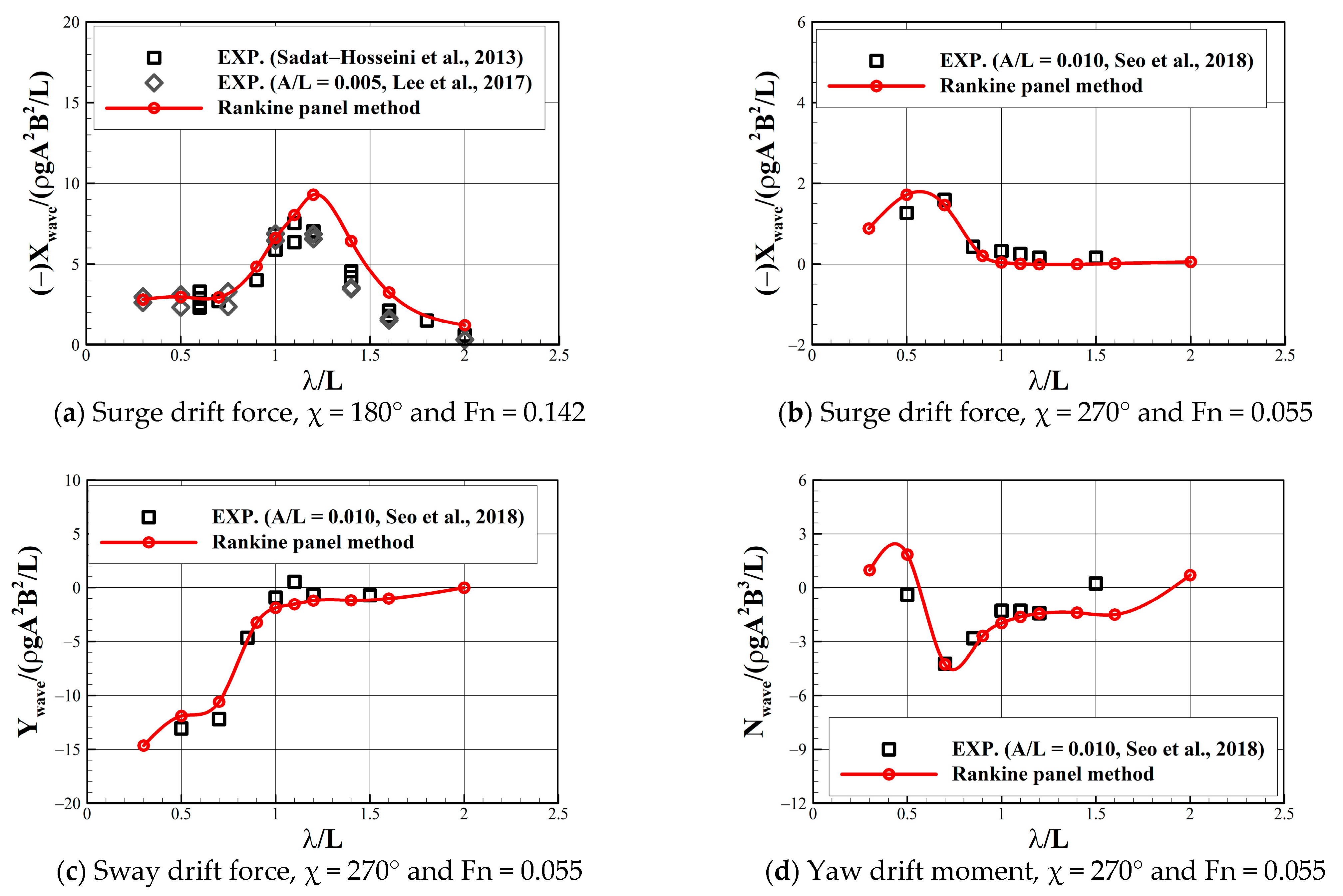
Seakeeping analysis was performed for the KVLCC2 tanker navigating in the constant operation velocities, and the Rankine panel method adopted in the present study was validated. The estimated surge, sway, and yaw drift force and moment were compared with the existing experimental data [27,28,29] and presented in Figure 2. It was observed that the applied Rankine panel method yielded results that agreed well with the experiment.
2.2. MMG Model (Maneuvering Analysis)
To describe the low-frequency ship maneuvering motion, a four degrees-of-freedom Maneuvering Modelling Group (MMG) model is adopted, which is defined with respect to the body-fixed coordinate system (o-xyz), as follows:
Here, m, Ixx, and Izz indicate the mass and the moments of inertia of a ship. X, Y, K, and N denote the surge, sway, roll, and yaw directional force and moment, and p0 is roll velocity. In the MMG model, the hydrodynamic forces induced by propeller rotation (Fpropeller), rudder deflection (FRudder), and ship operation (FHull) are calculated separately, whereas the mutual interaction between each component is considered by introducing several interaction coefficients. Moreover, the influence of the wave is taken into account by introducing second-order mean drift force and moment (Fwave). The MMG model adopted in this study is based on the hydrodynamic derivatives and interaction coefficients by [9] (S175) and [30] (KVLCC2). Details of the present MMG model are available in the abovementioned papers.
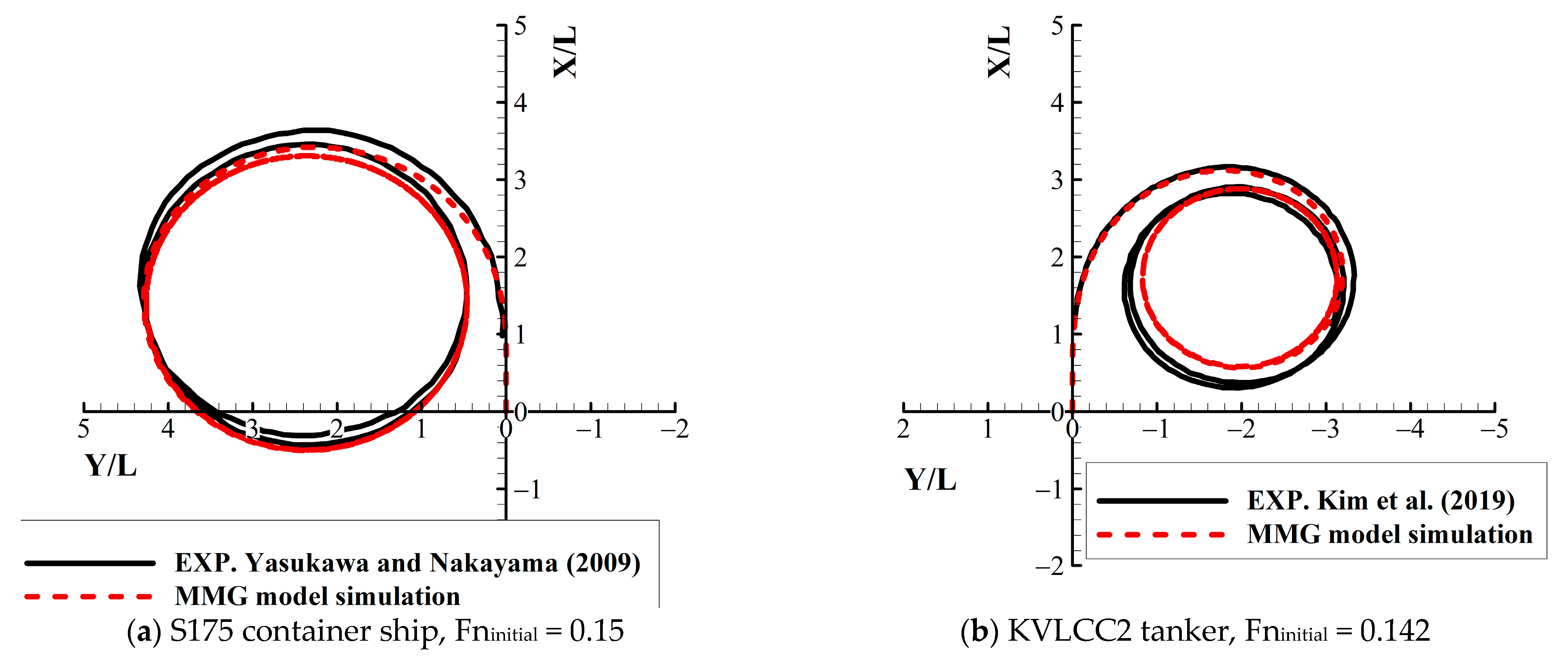
For validation, a 35° turning circle simulation was carried out and the trajectory obtained is shown in Figure 3. As shown in the turning trajectory, it can be observed that the applied MMG model reproduced the ship’s maneuvering motion.
2.3. Seakeeping-Maneuvering Coupling Analysis
In this paper, a modified two-time-scale model is proposed for a more realistic and efficient seakeeping-maneuvering coupling analysis, and its improvement is validated by comparing it with the existing two-time-scale model and direct coupling model. Three different numerical models, namely the modified two-time-scale model (MTM), direct coupling model (DCM), and existing two-time-scale model (ETM), are based on the same maneuvering equations, whereas the major difference between the three models is the manner in which wave drift force and moment are introduced, as follows:
Here, β0(=tan−1 (−v0/u0)) indicates the ship drift angle; χ, ω, and A denote wave heading, frequency, and amplitude, respectively. In the DCM, the seakeeping and maneuvering equations are solved simultaneously, and the physical quantities are exchanged at every time step. Concretely, the ship forward speed, steady drift, and yaw motion calculated by the maneuvering equations are considered in the evaluation of wave drift force and moment. The evaluated drift force is imposed on the maneuvering equations of motion such that the mean drift effect induced by the wave can be reflected in the assessment of ship operation velocities and the maneuvering trajectory. Because the seakeeping-maneuvering coupling procedure is directly performed at every time step, a more realistic analysis can be conducted by continuously updating the wave drift force and moment. On the other hand, based on the assumption that seakeeping and maneuvering equations can be solved independently, the ETM considers the wave effect by imposing a precomputed drift force. Furthermore, the effects of the steady drift and yaw motion are not reflected.
The MTM is proposed to improve the limitation of the existing two-time-scale model while retaining its computation time. The improvement is focused on a more realistic evaluation of the wave drift force and moment. The wave drift force is precomputed considering all directions of the ship operation velocities: forward speed, drift angle, and yaw rate. To reduce the burden of the seakeeping computation, the effects of the steady drift and yaw motion are considered independently. Moreover, by introducing up to the first-order derivative of Taylor series expansion, a bilinear model is applied for the variation in drift force caused by the steady drift and yaw motion, as shown in Equation (11).
Here, the linear derivative terms indicate the leading order variation of the wave drift force, which are functions of the ship forward speed and wave conditions. Based on the assumption that the effect of the ship steady drift and yaw motion on the surge directional drift force is negligible, a bilinear model is applied only to the sway and yaw directional force and moment. In addition, because the wave drift force exhibits an asymmetric trend with respect to the ship operation direction, a pair of coefficients are defined for certain forward speeds and wave conditions, as denoted in Equations (12) and (13).
where
In defining bilinear coefficients, appropriate β0 and r0 values must be selected to calculate the linear derivatives. If extremely small values are selected, the overall tendency of the wave drift force will not be represented well. Linear derivatives calculated by excessively large drift angles and yaw rates can result in overestimation. In this study, the drift angle and yaw rate values were selected based on the converged operation velocities in the calm water turning simulation, i.e., β0 = 0~10 [degree] (S175), β0 = 0~15 [degree] (KVLCC2) and r0 = 0~0.8 [degree/s] (S175, KVLCC2).
To obtain the linear derivative for the bilinear model, seakeeping analysis should be performed for a ship navigating in the constant operation velocities. However, in a real situation, the incident wave heading varies continuously when a ship operates at a steady yaw motion. Because the linear derivatives should be defined with respect to the specific incident wave heading, it is assumed that the wave heading remains constant during seakeeping computation, despite the presence of a steady yaw motion. In other words, the effect of the steady yaw motion on the encounter frequency and wave phase is assumed to be small when calculating the incident wave potential, similar to the [9].
where,
Here, k, ψ, and ε indicate wave number, turning angle, and phase, respectively.
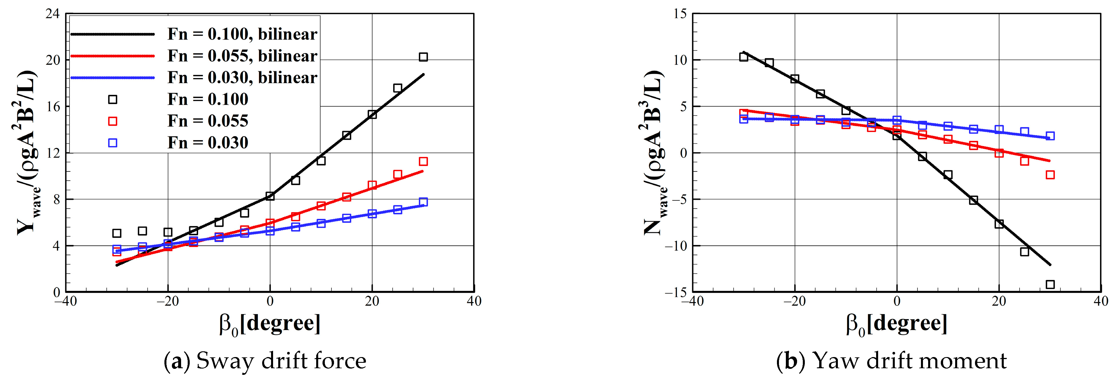
To investigate the validity of the MTM, wave drift force and moment were estimated by applying the bilinear model when a ship navigates in the constant forward and drift speed, and the results were compared with the values directly calculated by the Rankine panel method. Figure 4 shows sway drift force and yaw drift moment with respect to the ship drift motion, for the three different forward speeds of the KVLCC2 tanker. In these cases, the seakeeping computations were carried out for the regular short wave encountering in the bow-quartering region; λ/L = 0.7, χ = 120°. Although some discrepancies were revealed when the drift motion of a ship was excessive, the drift force estimated by the bilinear model agreed well with the results of the Rankine panel method.
3. Numerical Result
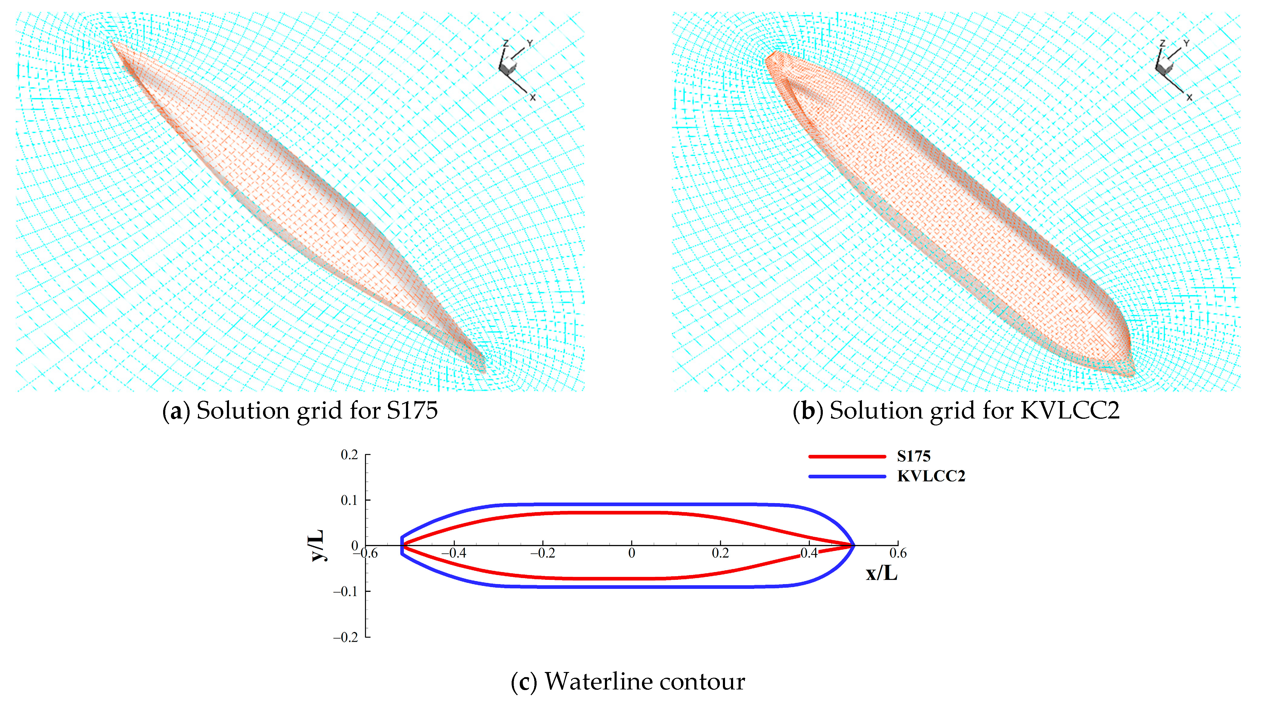
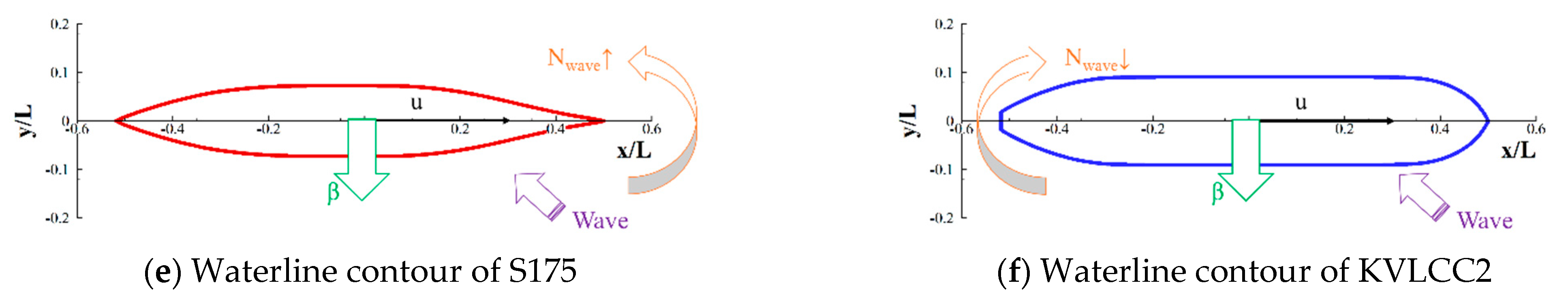
In this study, two different types of ship models—S175 container ship (CB = 0.572) and KVLCC2 tanker (CB = 0.810)—were chosen for maneuvering in wave analysis. Figure 5 shows the solution grids and waterline contours of the two target ship models. As shown in the Figure 5, the KVLCC2 tanker exhibits blunter waterline characteristics than the S175 container ship, particularly near the bow and stern shoulder region. Because the experimental data on the wave drift force and turning trajectories were released for both ship models, the numerical result obtained from the present study can be validated. The principal dimensions of the two ships are listed in Table 1.
In the present study, the maneuvering performance of the ship was evaluated for the short-wavelength condition λ/L = 0.7 to observe the remarkable global drift. The wave drift force and moment were calculated in the same wavelength condition, and Table 2 shows the forward speed and wave heading values for the seakeeping computation. The Froude number was selected to encompass the entire range of the ship forward speed during the maneuvering simulation, and a wave heading angle between 0° and 180° with a 30° interval was selected.
3.1. Characteristics of Bilinear Coefficients
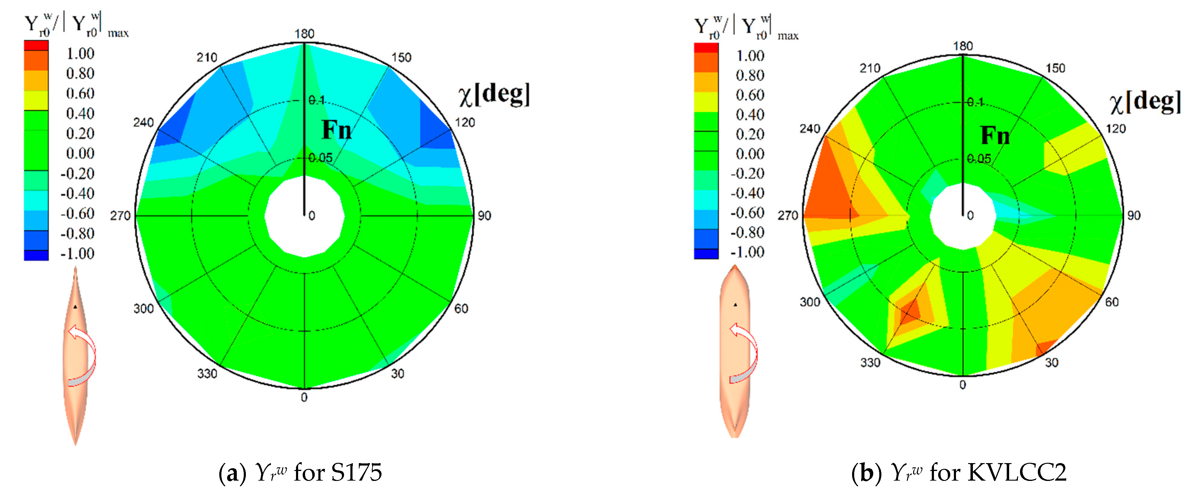
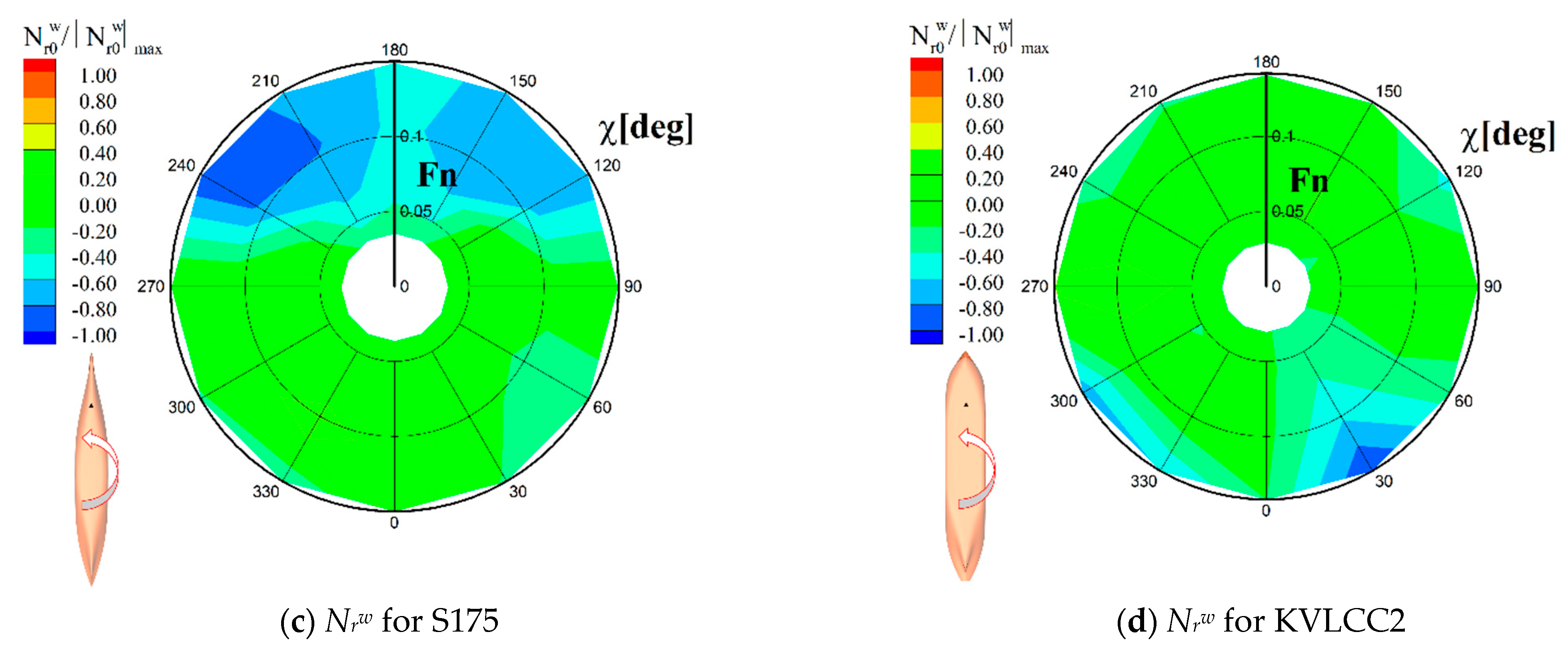
By comparing the characteristics of bilinear coefficients, the effects of the ship operation velocities on the wave drift force and moment are discussed. The defined bilinear coefficients represent the linear derivative of the drift force induced by the ship′s steady drift and yaw motion, and they are functions of the forward speed and wave heading. The dependency on the speed and heading was compared based on a polar contour, as seen in Figure 6 and Figure 7. In these figures, each coefficient was normalized by the maximum absolute value within the contour and their relative magnitude was compared with each other.
Overall, the magnitude of the bilinear coefficients became larger with the increasing forward speed and revealed asymmetric tendency regarding the operation directions. Figure 6 shows the bilinear coefficients related to the steady drift motion. It can be observed that Yβw always shows a positive value regardless of the operating condition, which indicates that the sway drift force increased in the opposite direction of drift motion for both ship models. On the other hand, the yaw drift moment varied differently with respect to the two target ships. The yaw drift moment of the S175 container ship increased in the opposite direction of the bow drift, whereas that of the KVLCC2 decreased. The variation of the drift force led by the steady yaw motion is shown in Figure 7. The yaw drift moment increased in the opposite direction of the steady yaw motion for both ship models. At the same time, the sway drift force exhibited a different tendency with respect to the ship models.
The difference in the bilinear coefficients between the two ship models is attributed to the characteristics of the hull geometry. Because the two ship models exhibit different waterline shapes, the relative wave elevation around the waterline varied differently. According to [31], relative wave elevation is the most significant factor for estimating the wave drift force and moment. Therefore, a variation of the drift force can be interpreted by investigating the distribution of wave elevation along the waterline.
Figure 8 shows the distribution of the relative wave elevation along the waterline varying with the steady drift motion when the wave was excited in the bow quartering region. When the wave was incident on the starboard side (χ = 120°), the relative wave elevation at the starboard remarkably increased due to the positive drift motion (the ship drifted toward the starboard side). The increment was especially prominent near the bow region for the S175 container ship and the stern shoulder region for the KVLCC2 tanker. On the other hand, the increment at the portside, which is the opposite side with respect to the wave excitation, was relatively small. Hence, the yaw drift moment increased in the opposite direction for the two ship models, although the sway drift force varied in the same direction.
In other words, the characteristics of the hull geometry affected the variation in wave drift force and moment induced by the ship operation, and contributed to the characteristics of the bilinear coefficients. The general property of the bilinear coefficients with respect to the hull geometry should be studied further.
3.2. Turning Circle Simulation in Regular Wave
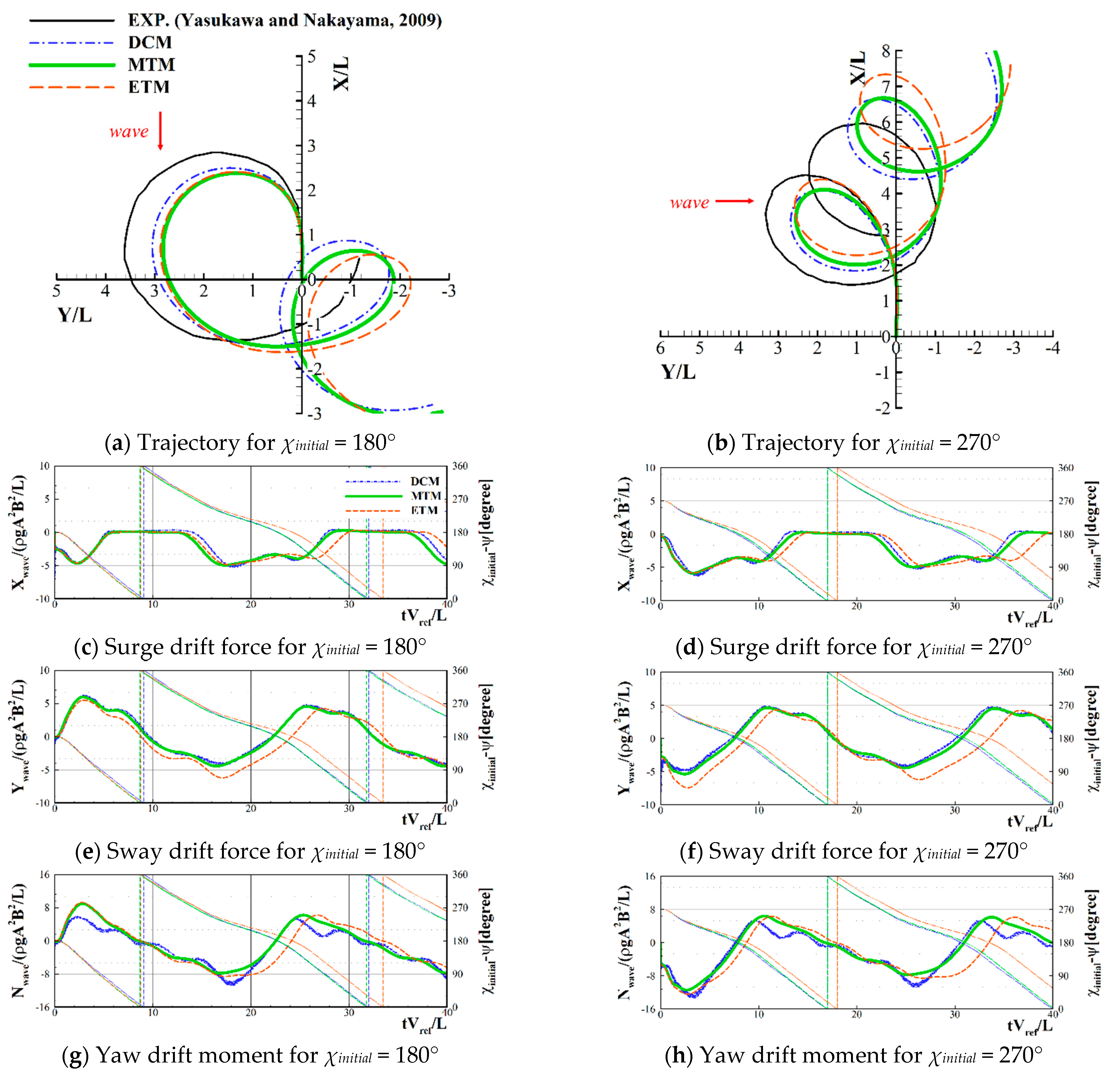
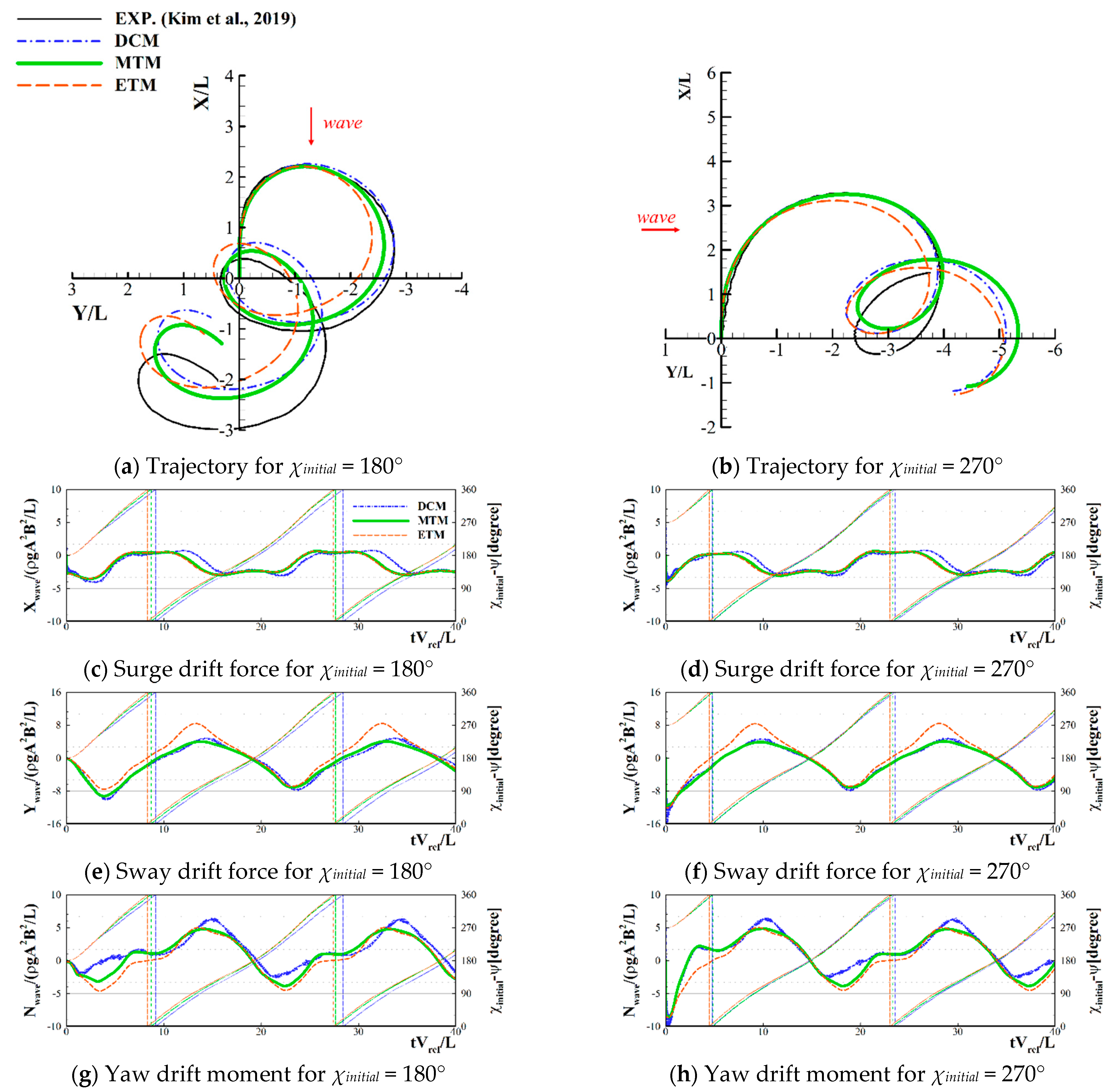
To validate the performance of the MTM, the turning circle simulation in regular waves was carried out. In the numerical simulation, propeller RPS was selected as the constant value corresponding to the ship design speed in calm water (Vref); RPS = 1.42 for S175 and RPS = 1.75 for KVLCC2. It should be noted that the additional steady force in the longitudinal direction induced by the waves—namely added resistance—leads to the decrement in the speed of a ship. Therefore, maneuvering simulation in the presence of the ocean waves started at the corresponding reduced speed, which is the same as the benchmark free-running experiment presented by [6,9]. In addition, the steering device was deflected until 35 degrees with a constant rotating speed. For the environmental conditions, the regular incident wave with λ/L = 0.7 and A/L = 0.01 was chosen, and two different values of the initial wave heading angles were selected (χinitial = 180°, 270°). Assuming the small amplitude of seakeeping properties, the linear seakeeping theory was applied for this simulation. The resultant turning trajectories and time histories of the drift force were compared with the DCM, and the improvement from the ETM is discussed.
Figure 9 shows the trajectories and wave drift force time histories of the S175 container ship, for χinitial = 180° and 270° and portside turning simulations. Compared with the DCM, the ETM showed vastly different trends of the drift force and moment, resulting in different turning trajectories. Meanwhile, the MTM, which introduces effects of the steady drift and yaw motion, yielded results similar to those of the DCM. By applying the MTM, the sway drift force was estimated much more accurately compared with the ETM, and the overall tendency of the yaw drift moment was similar to that obtained using the DCM. Although discrepancies in the yaw drift moment were observed at the bow quartering wave region, the global turning trajectory agreed well with the results obtained using the DCM.
Numerical simulation for the KVLCC2 tanker was conducted about the starboard turning, and the result is shown in Figure 10. In the case of the KVLCC2 tanker, agreements between the results of the DCM and free-running experimental data were much better than those of the S175 container ship. In addition, the global turning trajectory indicated an improvement by applying the MTM. A discrepancy in the yaw drift moment between the DCM and MTM was observed in the beam wave region, whereas the sway drift force of the two analysis models revealed good agreement.
By applying the MTM, the reliability of the prediction of ship maneuverability in regular waves was improved for both ship models. Because the MTM requires a computation time similar to that of the ETM, the MTM can be used as an efficient and reliable numerical tool for maneuvering in wave problems. The MTM required only a few seconds of time for the thousand seconds of maneuvering simulation, while the DCM took several hours; 20 h for KVLCC2 and 6 h for S175 (depending on the number of solution panels).
Meanwhile, the yaw drift moment showed a difference with that of the DCM, especially near the bow quartering wave region of the S175 container ship and the beam wave region of the KVLCC2 tanker. The discrepancy is mainly attributed to the characteristics of the bilinear model. Since the increment of the drift force induced by the steady drift and yaw motion was included up to the first-order derivative of Taylor series expansion, higher-order and coupling terms between the two operation velocities were not considered. Moreover, the MTM cannot take into account the memory effect, thus the continuous variation of the wave drift force and moment were not reflected. A more sophisticated mathematical model to overcome those limitations should be developed in the future.
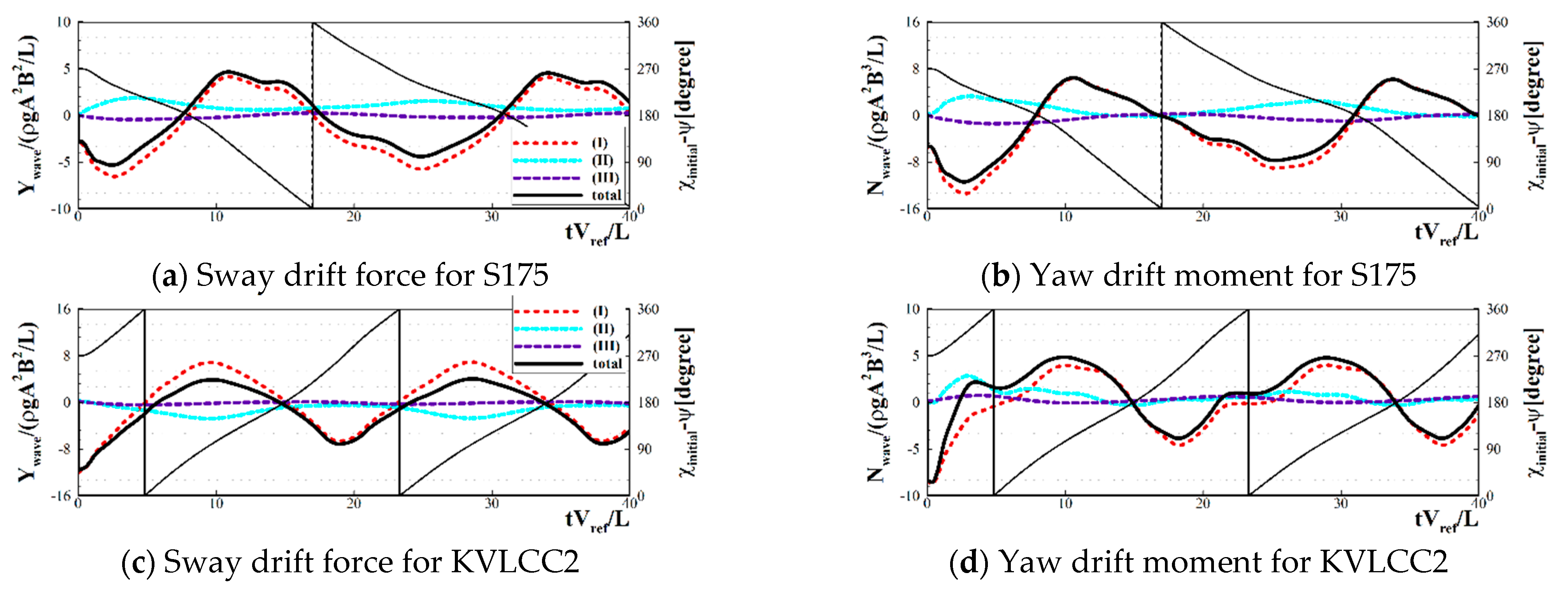
To investigate the relative contribution of the ship operation velocities, the time histories of the wave drift force and moment were decomposed into three components, as denoted in Equation (17). The first term indicates the wave drift force without the effects of the drift and yaw motion. The second and third terms denote the increment in the wave drift force and moment induced by the steady drift and yaw motion, respectively.
Figure 11 shows a comparison of the results for each component of the wave drift force estimated by the MTM, for a case of the initial beam wave excitation (χinitial = 270°). By considering the effects of the drift and yaw motion, it can be observed that the sway drift force and yaw drift moment were significantly affected. Especially, the influence of the drift motion was more remarkable than that of the yaw motion. Increment of the drift force and moment induced by the two operation velocities were most prominent in the bow quartering wave region of S175 container ship and the beam wave region of the KVLCC2 tanker. In other words, to more elaborately reflect the seakeeping-maneuvering coupling effects, all directions of operation velocities should be considered in evaluating the drift force and moment.
3.3. Drift Index
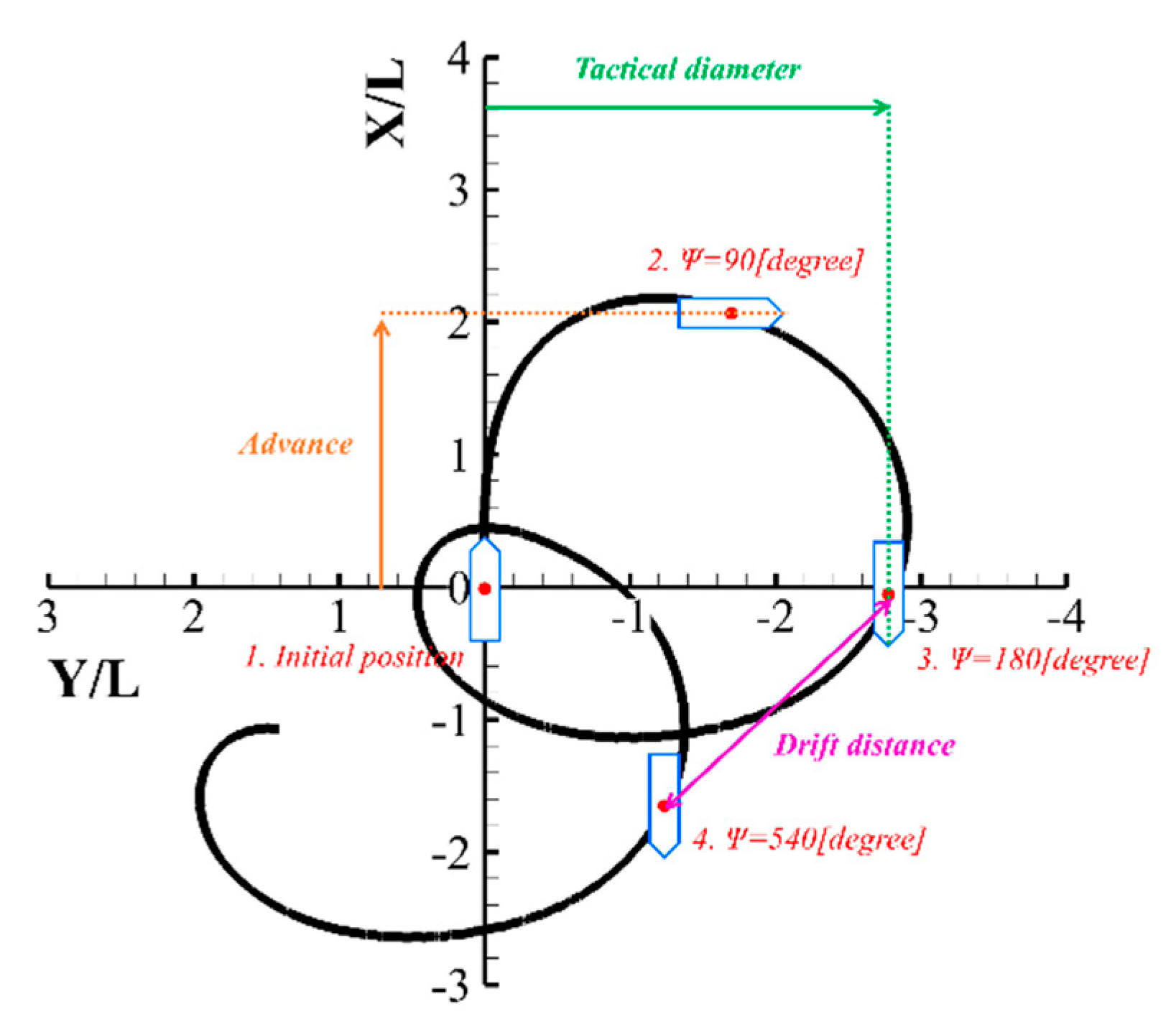
To quantitatively assess the performance of the MTM, several drift indices were defined and compared. In this study, three different types of drift indices (advance, tactical diameter, and drift distance) were adopted, and their definitions are shown in Figure 12. The advance/tactical diameter is defined as the x-/y-direction distance from the origin when the ship yaw angle is 90°/180°. The drift distance is defined as the distance between two ship positions in which the ship yaw angle becomes 180° and 540°, based on the study of [6].
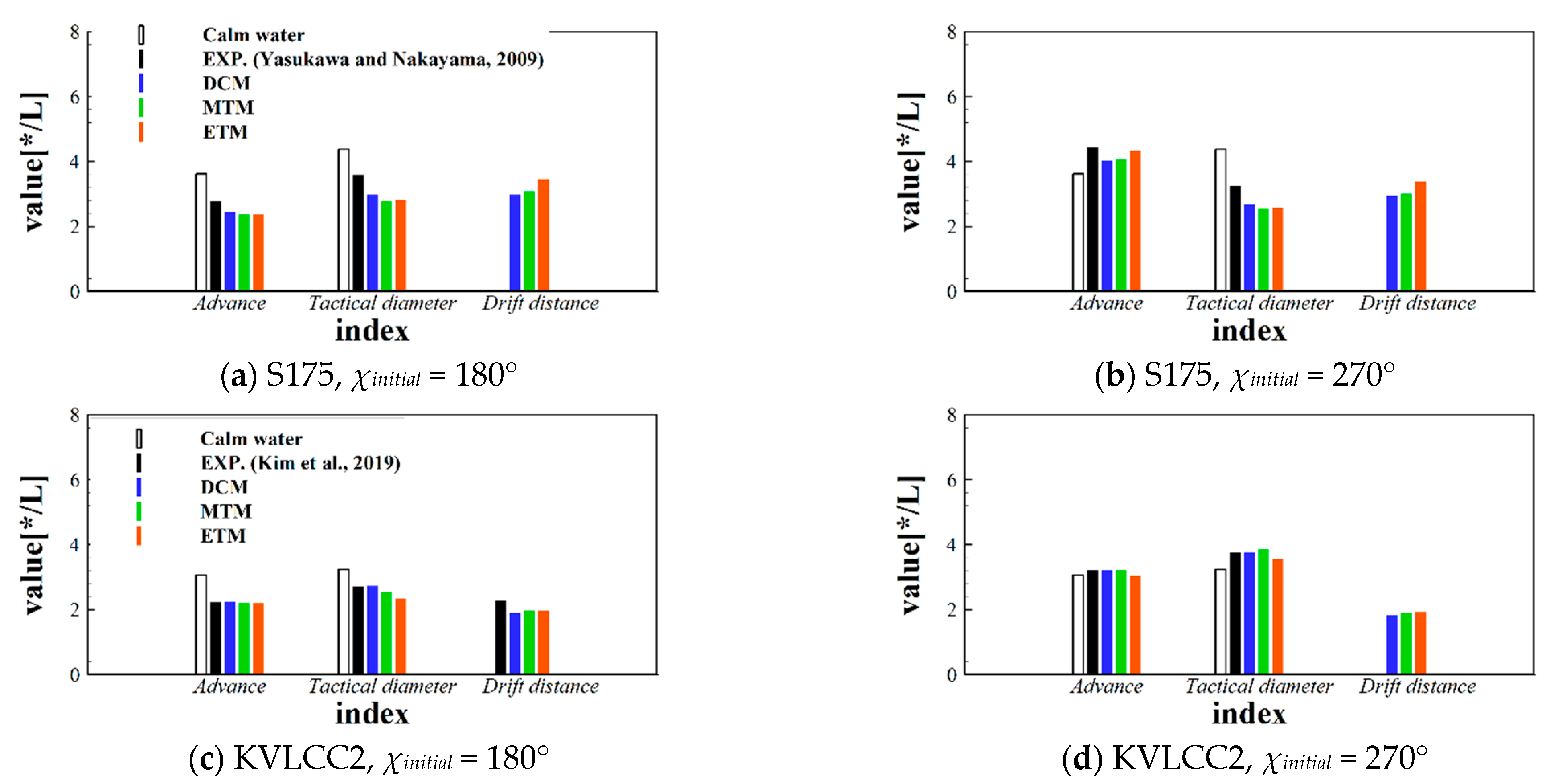
Figure 13 shows the drift indices of the S175 container ship and KVLCC2 tanker, respectively. Each index was normalized with respect to the ship length, and the results were visualized using a bar chart. Compared with the calm water maneuver, the advance and tactical diameter changed significantly in regular incident waves. In the initial head wave condition, both the advance and tactical diameter decreased. On the other hand, when the ship encountered a beam wave in the initial turning stage, the advance increased, and the tactical diameter varied differently based on the ship turning direction.
By comparing the drift indices estimated from the three different types of maneuvering analysis models, it was observed that the accuracy of the drift indices improved with the MTM. Improvement in the advance and tactical diameter of the S175 container ship was insignificant, even when the MTM was applied. However, the drift distance indicated a better agreement compared with that of the DCM. In the case of the KVLCC2 tanker, the result of the advance and tactical diameter evaluated using the MTM became more reliable, whereas improvement of the drift distance was trivial. In summary, reliability on the maneuvering analysis of a ship in regular waves was quantitatively improved, although overall trends of the improvement differed based on the ship models.
4. Conclusions
An MTM was proposed herein to develop a reliable and time-efficient numerical tool for the evaluation of ship maneuverability in regular waves. To this end, the effects of all components of ship operation velocities were reflected in the evaluation of the wave drift force and moment, and a bilinear model was applied to reduce the burden of the wave drift force computation. By applying the MTM, turning circle simulation in regular waves was conducted, and the performance was validated by comparing the results with those of the DCM. Based on the numerical results, the following conclusions were obtained:
- The effects of operation velocities on the drift force and moment were observed by comparing the bilinear coefficients and interpreted by investigating the relative wave elevation along the ship waterline. From the results, it was confirmed that the characteristics of the bilinear coefficients showed different tendencies based on the hull geometry.
- An MTM was applied for the evaluation of ship maneuverability in regular waves, and its performance was validated by comparing the turning trajectory and the time histories of drift force with those of the DCM. The numerical results of the MTM agreed well with the DCM, whereas a computation speed similar to that of the ETM was obtained.
- The relative contributions of the steady drift and yaw motion were investigated by comparing each component of the drift force and moment. Consequently, the effect of the steady drift motion was more prominent than that of the steady yaw motion in estimating ship maneuvering performance in waves.
- For the purpose of evaluating the quantitative performance of the MTM, several drift indices were defined and compared. Although the variation of the drift indices showed different tendencies based on the ship models, it can be concluded that the overall accuracy improved by applying the MTM.
Discrepancies between the DCM and MTM can be attributed to two reasons: the reflection of the memory effect and the limitation of the bilinear model. To improve the proposed MTM further, the main reason for the discrepancies should be investigated more concretely in the future. Moreover, although the bilinear model was applied, a considerable amount of drift force computation was required. In particular, it was unreasonable to apply the MTM for maneuvering in irregular waves. Hence, more efficient modifications should be developed in the future.
Author Contributions
Conceptualization, B.W.N. and Y.K.; methodology, J.L. and B.W.N.; software, J.L. and J.-H.L.; validation, J.L., J.-H.L. and B.W.N.; formal analysis, J.L., J.-H.L. and B.W.N.; investigation, J.L. and B.W.N.; resources, J.-H.L. and Y.K.; data curation, J.L. and J.-H.L.; writing—original draft preparation, J.L. and B.W.N.; writing—review and editing, Y.K.; visualization, J.L.; supervision, B.W.N. and Y.K.; project administration, Y.K.; funding acquisition, Y.K. All authors have read and agreed to the published version of the manuscript.
Funding
This study was funded by the Lloyd′s Register Foundation (LRF)-Funded Research Center at Seoul National University, project number GA 10050.
Institutional Review Board Statement
Not applicable.
Informed Consent Statement
Not applicable.
Data Availability Statement
The data presented in this study were available in this article (Tables and Figures).
Acknowledgments
Authors appreciate the support of the Lloyd’s Register Foundation Center in Seoul National University.
Conflicts of Interest
The authors declare no conflict of interest.
References
- International Maritime Organization (IMO). 2013 Interim Guidelines for Determining Minimum Propulsion Power to Maintain the Manoeuvrability of Ships in Adverse Conditions; MEPC.232 (65); IMO: London, UK, 2013.
- Papanikolaou, A.; Zaraphonitis, G.; Bitner-Gregersen, E.; Shigunov, V.; El Moctar, O.; Soares, C.G.; Reddy, D.; Sprenger, F. Energy efficient safe ship operation (SHOPERA). Transp. Res. Procedia 2016, 14, 820–829. [Google Scholar] [CrossRef] [Green Version]
- Shigunov, V.; El Moctar, O.; Papanikolaou, A.; Potthoff, R.; Liu, S. International benchmark study on numerical simulation methods for prediction of manoeuvrability of ships in waves. Ocean Eng. 2018, 165, 365–385. [Google Scholar] [CrossRef]
- Yasukawa, H. Simulation of wave-induced motions of a turning ship. J. Jpn. Soc. Nav. Archit. Ocean Eng. 2006, 4, 117–126. [Google Scholar]
- Sanada, Y.; Tanimoto, K.; Takagi, K.; Gui, L.; Toda, Y.; Stern, F. Trajectories for ONR Tumblehome maneuvering in calm water and waves. Ocean Eng. 2013, 72, 45–65. [Google Scholar] [CrossRef]
- Kim, D.J.; Yun, K.; Park, J.-Y.; Yeo, D.J.; Kim, Y.G. Experimental investigation on turning characteristics of KVLCC2 tanker in regular waves. Ocean Eng. 2019, 175, 197–206. [Google Scholar] [CrossRef]
- Yasukawa, H.; Hirata, N.; Yonemasu, I.; Terada, D.; Matsuda, A. Maneuvering simulation of a KVLCC2 tanker in irregular waves. In Proceedings of the International Conference on Marine Simulation and Ship Maneuverability, Newcastle, UK, 8–11 September 2015. [Google Scholar]
- Skejic, R.; Faltinsen, O.M. A unified seakeeping and maneuvering analysis of ships in regular waves. J. Mar. Sci. Technol. 2008, 13, 371–394. [Google Scholar] [CrossRef]
- Yasukawa, H.; Nakayama, Y. 6-DOF motion simulations of a turning ship in regular waves. In Proceedings of the International Conference on Marine Simulation and Ship Manoeuvrability, Panama City, Panama, 17–20 August 2009. [Google Scholar]
- Chillcce, G.; el Moctar, O. A numerical method for manoeuvring simulation in regular waves. Ocean Eng. 2018, 170, 434–444. [Google Scholar] [CrossRef]
- Schoop-Zipfel, J. Efficient Simulation of Ship Maneuvers in Waves. Ph.D. Thesis, Technische Universität Hamburg, Hamburg, Germany, 2017. [Google Scholar]
- Hassani, V.; Ross, A.; Selvik, Ø.; Fathi, D.; Sprenger, F.; Berg, T.E. Time domain simulation model for research vessel Gunnerus. In Proceedings of the International Conference on Offshore Mechanics and Arctic Engineering, St. John’s, NL, Canada, 31 May–5 June 2015. [Google Scholar]
- Wicaksono, A.; Kashiwagi, M. Efficient coupling of slender ship theory and modular maneuvering model to estimate the ship turning motion in waves. In Proceedings of the 29th International Ocean and Polar Engineering Conference, Honolulu, HI, USA, 16–21 June 2019. [Google Scholar]
- Skejic, R.; Faltinsen, O.M. Maneuvering behavior of ships in irregular waves. In Proceedings of the International Conference on Offshore Mechanics and Arctic Engineering, Nantes, France, 9–14 June 2013. [Google Scholar]
- Xu, Y.; Bao, W.; Kinoshita, T.; Itakura, H. A PMM experimental research on ship maneuverability in waves. In Proceedings of the International Conference on Offshore Mechanics and Arctic Engineering, San Diego, CA, USA, 10–15 June 2007; pp. 11–16. [Google Scholar]
- Adnan, F.; Yasukawa, H. Experimental investigation of wave-induced motions of an obliquely moving ship. In Proceedings of the 2nd Regional Conference on Vehicle Engineering and Technology, Kuala Lumpur, Malaysia, 15–16 July 2008. [Google Scholar]
- Seo, M.-G.; Nam, B.W.; Kim, Y.-G. Numerical Evaluation of Ship Turning Performance in Regular and Irregular Waves. J. Offshore Mech. Arct. Eng. 2020, 142, 021202. [Google Scholar] [CrossRef]
- Seo, M.-G.; Kim, Y. Numerical analysis on ship maneuvering coupled with ship motion in waves. Ocean Eng. 2011, 38, 1934–1945. [Google Scholar] [CrossRef]
- Zhang, W.; Zou, Z.-J.; Deng, D.-H. A study on prediction of ship maneuvering in regular waves. Ocean Eng. 2017, 137, 367–381. [Google Scholar] [CrossRef]
- Lee, J.-H.; Kim, Y. Study on steady flow approximation in turning simulation of ship in waves. Ocean Eng. 2020, 195, 106645. [Google Scholar] [CrossRef]
- Fossen, T.I. A nonlinear unified state-space model for ship maneuvering and control in a seaway. Int. J. Bifurc. Chaos. 2005, 15, 2717–2746. [Google Scholar] [CrossRef]
- Bailey, P. A unified mathematical model describing the maneuvering of a ship travelling in a seaway. Trans RINA 1997, 140, 131–149. [Google Scholar]
- Lee, J.; Nam, B.W.; Lee, J.-H.; Kim, Y. Development of new two-time-scale model for ship manoeuvring in waves. In Proceedings of the 31th International Ocean and Polar Engineering Conference, Rhodes, Greece, 20–25 June 2021. [Google Scholar]
- Lee, J.-H.; Kim, B.-S.; Kim, Y. Study on steady flow effects in numerical computation of added resistance of ship in waves. J. Adv. Res. Ocean Eng. 2017, 3, 193–203. [Google Scholar]
- Shao, Y.-L.; Faltinsen, O.M. Linear seakeeping and added resistance analysis by means of body-fixed coordinate system. J. Mar. Sci. Technol. 2012, 17, 493–510. [Google Scholar] [CrossRef]
- Kim, Y.; Kim, K.-H.; Kim, J.-H.; Kim, T.; Seo, M.-G.; Kim, Y. Time-domain analysis of nonlinear motion responses and structural loads on ships and offshore structures: Development of WISH programs. Int. J. Nav. Archit. Ocean Eng. 2011, 3, 37–52. [Google Scholar] [CrossRef] [Green Version]
- Sadat-Hosseini, H.; Wu, P.-C.; Carrica, P.M.; Kim, H.; Toda, Y.; Stern, F. CFD verification and validation of added resistance and motions of KVLCC2 with fixed and free surge in short and long head waves. Ocean Eng. 2013, 59, 240–273. [Google Scholar] [CrossRef]
- Lee, J.; Park, D.-M.; Kim, Y. Experimental investigation on the added resistance of modified KVLCC2 hull forms with different bow shapes. Proc. Inst. Mech. Eng. Part M J. Eng. Marit. Environ. 2017, 231, 395–410. [Google Scholar] [CrossRef]
- Seo, M.-G.; Nam, B.W.; Yeo, D.J.; Yun, K.; Kim, D.J.; Park, J.Y.; Kim, Y.-G. Numerical analysis of turning performance of KVLCC2 in regular waves. In Proceedings of the Annual Autumn Conference, SNAK, Changwon, Korea, 24–26 October 2018. [Google Scholar]
- Yasukawa, H.; Yoshimura, Y. Introduction of MMG standard method for ship maneuvering predictions. J. Mar. Sci. Technol. 2015, 20, 37–52. [Google Scholar] [CrossRef] [Green Version]
- Kim, K.-H.; Kim, Y. Numerical study on added resistance of ships by using a time-domain Rankine panel method. Ocean Eng. 2011, 38, 1357–1367. [Google Scholar] [CrossRef]
Figure 1.
Coordinate definition for the seakeeping analysis.

Figure 2.
Wave drift force and moment for the KVLCC2 tanker.

Figure 3.
Turning trajectories in calm water.

Figure 4.
Validation results of the bilinear model.

Figure 5.
Solution grids and waterline contour.

Figure 6.
Polar contour of the β-coefficients.

Figure 7.
Polar contour of the r-coefficients.


Figure 8.
Distribution of relative wave elevation amplitude when χ = 120°.


Figure 9.
Turning trajectories and time histories for the S175 container ship: RPS = 1.42.

Figure 10.
Turning trajectories and time histories for the KVLCC2 tanker: RPS = 1.75.

Figure 11.
Time histories of the wave drift force and moment (contribution of β0 and r0).

Figure 12.
Definition of the drift indices.

Figure 13.
Drift indices.


Table 1.
Principal dimensions of ship models.
| Definition | S175 Container Ship | KVLCC2 Tanker |
|---|---|---|
| Length [m] | 175.0 | 320.0 |
| Breadth [m] | 25.4 | 58.0 |
| Draft [m] | 9.5 | 20.8 |
| Block coefficient | 0.572 | 0.810 |
Table 2.
Simulation cases for wave drift force and moment computation.
| S175 Container Ship | KVLCC2 Tanker | |
|---|---|---|
| Froude number | 0.036, 0.072, 0.110, 0.150 | 0.030, 0.055, 0.100, 0.142 |
| Wave heading | χ = 0~180° (30° interval) | |
Publisher’s Note: MDPI stays neutral with regard to jurisdictional claims in published maps and institutional affiliations. |
© 2021 by the authors. Licensee MDPI, Basel, Switzerland. This article is an open access article distributed under the terms and conditions of the Creative Commons Attribution (CC BY) license (https://creativecommons.org/licenses/by/4.0/).
Share and Cite
MDPI and ACS Style
Lee, J.; Nam, B.W.; Lee, J.-H.; Kim, Y. Development of Enhanced Two-Time-Scale Model for Simulation of Ship Maneuvering in Ocean Waves. J. Mar. Sci. Eng. 2021, 9, 700. https://doi.org/10.3390/jmse9070700
AMA Style
Lee J, Nam BW, Lee J-H, Kim Y. Development of Enhanced Two-Time-Scale Model for Simulation of Ship Maneuvering in Ocean Waves. Journal of Marine Science and Engineering. 2021; 9(7):700. https://doi.org/10.3390/jmse9070700
Chicago/Turabian StyleLee, Jaehak, Bo Woo Nam, Jae-Hoon Lee, and Yonghwan Kim. 2021. "Development of Enhanced Two-Time-Scale Model for Simulation of Ship Maneuvering in Ocean Waves" Journal of Marine Science and Engineering 9, no. 7: 700. https://doi.org/10.3390/jmse9070700
Note that from the first issue of 2016, this journal uses article numbers instead of page numbers. See further details here.