Article

A High-Resolution Numerical Model of the North Aegean Sea Aimed at Climatological Studies

1
Department of Marine Sciences, School of the Environment, University of the Aegean, 81100 Mytilene, Greece
2
Hellenic Centre for Marine Research, Operational Oceanography Group, Institute of Oceanography, 19013 Attica, Greece
*
Author to whom correspondence should be addressed.
J. Mar. Sci. Eng. 2021, 9(12), 1463; https://doi.org/10.3390/jmse9121463
Submission received: 23 November 2021 / Revised: 15 December 2021 / Accepted: 16 December 2021 / Published: 20 December 2021
(This article belongs to the Special Issue Hydrodynamic Circulation Modelling in the Marine Environment)

Abstract

:
A new, high-resolution model for the northern part of the Aegean Sea, aimed primarily at climatological research (relaxation and data assimilation-free climate simulations), is hereby presented, along with the results of a 28-year-long simulation covering the period from 1986 to 2013. The model applied is the Regional Ocean Modelling System (ROMS). A significant improvement over previous models of the Aegean introduced in this work is the replacement of parameterizations of the Dardanelles exchange by a fully three-dimensional simulation of the flow in the Strait. The incorporation of part of the Marmara Sea in the model domain enables the interaction with other regional climate simulations, thus allowing climatic variability of the exchange of the Mediterranean and Black Seas. An extensive validation is carried out comparing the model output with all the available observations from several different platforms, i.e., satellite sea surface temperature and height, T/S profiles from R/V ships, and HF radar surface currents velocity. We focus on the model’s ability to reproduce, to some extent, the distinct thermohaline features and circulation patterns that characterize this specific area of the Mediterranean Sea. Our findings, after comparing simulation results with all the available observations, revealed the model’s sufficiency to simulate very adequately the complex hydrology of the North Aegean Sea, and the model’s ability to reproduce incidents of deep-water formation that took place in the region in previous decades during the Eastern Mediterranean Transient (EMT).

1. Introduction

The North Aegean Sea is one of the most intriguing seas of the Mediterranean, being the first receptor of waters from the Black Sea through the so-called Turkish Strait System (TSS), comprising the Dardanelles and Bosphorus Straits and the Marmara Sea). While it is one of the northernmost extremities of the basin, and thus, an alternative source of Eastern Mediterranean Deep Waters (EMDW), along with the Adriatic Sea [1,2], the inflow of very light, low-salinity waters from the Black Sea through the TSS plays a critical role in controlling deep-water formation over the basin for the following reasons: (a) the lateral buoyancy inflow through the Dardanelles reduces surface density and increases stratification, hindering the formation of very dense waters, and (b) the Black Sea Waters (BSW) form a thin surface layer, colder than its underlying waters of Aegean/Levantine origin, a condition minimizing heat losses to the atmosphere in the winter [3]. This critical role of the Dardanelles outflow in controlling overturning processes in the North Aegean was proposed after it was recognised that the massive Eastern Mediterranean Transient (EMT) was triggered in 1987 in this basin [2,4], although the involved processes were not fully understood at the time. The above event shook the until-then established perception of the Eastern Mediterranean, overturning circulation and demonstrating that the Aegean Sea has the capacity to become a major dense-water formation site and an alternative producer of Eastern Mediterranean Deep Water (EMDW) [5].
The inflow of Black Sea waters in the North Aegean plays a crucial role in controlling not only overturning processes, but also circulation [6], as well as ecosystem functioning and productivity [7,8,9] of the basin, which also explains the fact that most Greek coastal fishery takes place in the North Aegean [10]. Thus, the development of a numerical model suitable for climatological studies of the North Aegean would require a simulation of the interannual variability of the Dardanelles inflow of BSW. Until now, most simulations of the circulation of the Aegean Sea have been aimed mainly for operational oceanography applications [11,12,13,14], for which parameterizations of the seasonal cycle of the Dardanelles exchange [15] are considered adequate.
More recent works have treated the Dardanelles exchange as an open boundary exhibiting only seasonal variability of the exchanged volume rates [16], while the temperature characteristics of the inflowing BSW have been allowed to vary interannually based on observational data [17]. In an effort to address interannual variability of the Dardanelles outflow, Androulidakis et al. [18] have exploited the water budget of the Black Sea throughout the period 2002–2003, while in a more recent work, Mavropoulou et al. [19] showed that the interannual variability of the Dardanelles outflow plays a little role in the general circulation of the North Aegean, although it can have an important impact in the water column structure.
The present work extends the domain of the numerical simulation of the North Aegean Sea into the Marmara Sea to enable the application of open boundary conditions there, obtained from any regional-scale simulations available for the period of interest. In the present application of the model, simulating the period 1986–2013, we have used results from a TSS analytical model covering that period [20].

2. Materials and Methods

2.1. Model Description

We have employed the Regional Ocean Modelling System (ROMS), a free-surface, hydrostatic, primitive equation model, widely used by the scientific community for a diverse range of applications [21,22]. A rectangular grid of 1.0 km resolution with 31 vertical sigma levels covering the North Aegean Sea area—black square area (Figure 1)—was developed using General Bathymetric Charts of the Ocean (GEBCO) 2014 bathymetry. To ensure the hydrostatic consistency of the grid (minimizing perturbation), we have used a linear programming method [23] to smooth bathymetry and set the ROMS’ bathymetric smoothing parameters rx0 [24] and rx1 [25] equal to 0.125 and 6.91, respectively.
For momentum advection, we have used the 3rd-order upstream split scheme [26,27,28] as implemented in the ROMS model. This choice came after several sensitivity test runs mainly focused on the Turkish Straight System (TSS). The latter scheme gave the smallest Bias and Root-Mean-Square-Error (RMSE) and mainly a more realistic representation of the steep T/S distribution in the vicinity of the Dardanelles exit, compared to the default 3rd-order upstream Bias scheme. For tracer advection, the Multidimensional Positive Definite Advection Transport Algorithm (MPDATA) scheme [29], with a weak harmonic operator along constant geopotential surfaces, was used. The vertical mixing scheme was the classical Mellor, Yamada 2.5 [30], using the default background values for eddy viscosity and diffusivity. For the bottom stresses, a quadratic bottom drag scheme was applied using the model default value (of 3 × 10⁻³). The selection for bottom-stress type and its value came after several sensitivity-test runs and the previous combination gave the slightly smallest Root Mean Square Error (RMSE) for sea surface height when compared with altimetric data for sea level anomaly.
Initial conditions for temperature and salinity came from a Mediterranean Sea hydrographic atlas [31]. The T/S data combined with ERA5 [32] winds were used to estimate the initial values for the baroclinic geostrophic and Ekman velocity components, setting a level of no motion at 600 m depth to determine the total velocity. Boundary conditions for the south side of the computational grid were provided by a basin scale model of the Mediterranean Sea distributed from CMEMS [33] on a daily resolution. Data for the eastern boundary, located at the western extremity of Marmara Sea, were derived from the work of V. Maderich [19], providing temperature, salinity, sea surface height and volume flux time series for both inflow and outflow layers on a daily basis. At all open boundaries, mixed radiation—nudging conditions [34]—were used for 3D fields (T, S, u, v), Chapman [35] for free surface (ζ) and Flather [36] for barotropic velocities (ubar, vbar). Riverine inputs from the 8 larger rivers outflowing in the Aegean were provided in the form of a climatological time series from the SMHI e-hype hydrological model [37], covering the period from 1980 to 2010. Atmospheric forcing of ¼-degree spatial resolution and 1 h temporal resolution came from the European Centre for Medium-range Weather Forecast (ECMWF) ERA5 reanalysis dataset and was incorporated in the model using the COARE bulk formulae [38].
The atmospheric forcing used consisted of wind velocity components at 10 m height, 2 m height air temperature, dewpoint temperature (to calculate relative humidity) at 2 m height, mean sea level pressure, total rainfall, net shortwave radiation, and downwards longwave radiation.
The simulation covers the period from 1 January 1985 to 1 January 2014. The model was initialized with a cold start on 1 January 1985. The first year (from 1 January 1985 until 31 December 1985) is considered the spin-up period and the results were excluded from our analysis. Finally, it should be noted that our experiment excluded any kind of relaxation (climatological or atmospheric).

2.2. Data for Model Validation

Various sources of oceanographic information have been used to validate the model. Sea-surface temperature information was provided by the Copernicus Marine Environment Monitoring Service (CMEMS-SST GLO SST L4 REP OBSERVATIONS 010 024, [39]) for the period 1986 to 2013, and an ultra-high resolution SST product [40] for the year 2010. Sea Level Anomaly (SLA) and Mean Dynamic Topography (MDT) were also provided by CMEMS (product names SEALEVEL MED PHY L4 REP OBSERVATIONS 008 051, SSALTO DUACS, SEALEVEL MED PHY MDT L4 STATIC 008 066). Historical data of temperature and salinity covering the 28-year period came from SeaDataNet database (Mediterranean Sea–Temperature and salinity Historical Data Collection SeaDataCloud V2 [41]). The validation of the model is extended to surface current information from the northeast Aegean, the immediate receptor of Black Sea Waters in flowing into the Aegean Sea through the Dardanelles Strait. This region is covered by the WERA-type High-Frequency radar “Dardanos”, with information provided for the year 2010, January–June 2011 and July–August 2021. Of course, the ocean currents from the HF radar cover a much smaller geographical area than the numerical domain of the simulation, however, our validation with this source of information is important for several reasons, such as reproducing exchange fluxes between the two seas, simulating regional dynamics, as well as developing tools for coastal pollution management and search-and-rescue (SAR) operations.

2.3. Methods for Model Validation

A crucial post-process following the completion of the numerical simulations is the estimation of the model’s statistical error. To that aim, we extensively validated our results with all available information; satellite data (Sea Surface Temperature and Sea Level Anomaly), in situ (T/S profiles from R/Vs) and HF radar surface velocity fields. The model’s error for each run was estimated using standard statistical metrics such as Root Mean Square Error (RMSE), Bias skill, Pearson correlation coefficient and Murphy skill score [42] as a model skill index when compared with altimetry data. The significance of each statistical metric used is dependent on the nature of the investigated parameter: for example, in comparing modelled and observed T/S profiles, RMSE and Bias skill offer a more thorough understanding than correlation coefficient or Murphy Skill score.
One of the criteria used to evaluate the model’s performance is the ability to reproduce the surface circulation. As the broadest spatiotemporal coverage for surface circulation is provided from satellite altimetry and the consequent calculation of geostrophic currents, this method was chosen for the comparison with simulated currents in the North Aegean.
The kinetic energy of the surface geostrophic currents is obtained from the model’s sea surface height output ( ζ ) using a finite differences approach for the geostrophic approximation
u g = g f ζ y
v g = g f ζ x
K E = 1 2 u g 2 + v g 2
where u g and v g are the zonal and meridional components of the geostrophic velocity, g is the gravitational acceleration and f the Coriolis parameter. The same procedure is followed for the estimate of kinetic energy using sea surface heights derived from satellite observations: Absolute Dynamic Topography (ADT) was obtained as the sum of SLA plus the multiyear climatological MDT, covering the period from 1992 to 2012 for the Mediterranean Sea.

3. Results

3.1. Model Validation

3.1.1. Sea-Surface Temperature

Initially we compared the sea surface temperature (SST) of our model to high resolution Level 4 reprocessed satellite SST data. The results from our analysis are shown in Figure 2. The region exhibiting the poorest performance of the model is the vicinity of the Dardanelles exit to the Aegean Sea, as revealed by both Bias and RMSE indices (Figure 2a,b). The complexity of the Turkish Straits System and, especially, the hydraulic control that occurs at the Nara Passage [17,43] combined with the hydrostatic nature of the model—although the number of vertical levels is high—pushes the vertical mixing scheme locally to its limits. This results in a mismatch between the modelled and the observed values, but not for all months, as can be seen from Figure 3, where the seasonal RMSE from the mean climatological year as calculated from the model’s results are presented. The error seems to be systematic and tends to decrease during the year with higher values during winter months and lower during autumn. Figure 4 shows the interannual variability and linear trends of SSTs from satellite observations and model results. Trend values from model results are lower (0.038 °C/year) compared to the satellite data trend (0.054 °C/year). Although the numbers are of the same order of magnitude, the lower trend of the simulations seems to be due to the initial overestimation of the SST. Nonetheless, most of the variability remains within the confidence interval, as defined by one standard deviation of the satellite observations, even during the years of 1992 and 1993 when the EMT peaked.
From the above figures, we conclude that our model tends to overestimate the sea surface temperature with a positive bias, both interannually and seasonally, but for a 28-year long simulation the magnitude of error RMSE and Bias is considered acceptable for a free run. Overall, the model satisfactorily reproduces the interannual and intra-annual SST variability, with a Murphy skill score approximately equal to 0.97 on the SST’s evolution full signal and 0.92 after removing the seasonal cycle.
The southwest-northeast direction of the increased SST differences in the Dardanelles area (Figure 2 and Figure 3) can be attributed to the misrepresentation of the southward extent and the path, followed by the BSW plume by the model, mainly affected by the uncertainty of volume inflow at the Dardanelles Strait and the influence of wind forcing.
In fact, we should stress that the area east of Lemnos (the Lemnos Plateau) hosts the strongest frontal zone in the Aegean Sea [44]. The inflow of BSW creates a thin, buoyant layer of brackish water in the Dardanelles area [17] which, owing to its small depth, responds rapidly to changes of wind stress [45]. Wind forcing also affects the position and extent of the Samothraki anticyclone [46], the south-eastern flank of which may contribute significantly to the circulation of the northern part of the Lemnos Plateau [47]. Under the influence of north winds, the path of the BSW bifurcates and its southern branch circulates around Lemnos Island. To the south, the BSW is bound by Levantine-originated waters, carried northward by the general cyclonic circulation of the Aegean Sea [48]. Except for during the summer season, the BSW can be identified in SST images by its low temperature signal [49]. During summer, the dominant north winds in the area cause upwelling in the eastern coasts of the Aegean Sea [50,51]. Two of the upwelling centres, easily spotted in the historical satellite SST images during summer, are in the vicinity of the Dardanelles area; one along the Turkish coast south of the Dardanelles exit and another at the west coasts of Lesvos Island [52]. Moreover, the intensity of wind curl and the response to Ekman transport are linked to the intrusion of the Levantine-originated waters from the south-eastern part of the Aegean Sea further to the north [53,54].
To investigate the increased differences between the model and satellite SSTs, we have used the available observations of surface currents from the HF radar during August 2010 and August 2021 in conjunction with satellite observations for the 2006–2009 and 2010–2013 periods. For the 2006–2009 period, lateral boundary conditions are the results of the numerical simulations by Maderich et al. [20]. During 2010–2013, the climatology of the 1986–2009 results by the same authors is used.
Note that the wind conditions during August 2010 are markedly different from those during August 2021 (Figure 5c,g). A stronger Ekman transport during 2010 intensified the Samothraki anticyclone and moved its east flank to the west, between Lemnos and Imvros islands (Figure 5d,h). The cold upwelled waters of the eastern coasts of the central Aegean were transported to the southern part of the area measured by the radar (Figure 5b), where they formed a frontal region of strong convergence (Figure 5a). During 2021, the influence of the anticyclone of Samothraki was found between Imvros and the Dardanelles exit (Figure 5h). Cold waters moving to the west from the upwelling centre to the southeast of Tenedos Island can be observed in Figure 5f. The convergence region has moved northwards, and its direction has changed with respect to that of August 2010 (Figure 5e). As the region of the largest model SST error is aligned with the thermal front and drops moving away from it for both periods (2006–2009, 2010–2013), the model error increased for the period forced by the climatological field (Figure 5i–l), and taking into account that the interannual variability of the BSW is larger than the seasonal variability [20], we conclude that the largest part of the model SST error in this region is caused by the misrepresentation of the position of the plume of BSW, attributed to the combination of the uncertainty of BSW inflow, the low spatial resolution of wind forcing and the artificial numerical mixing at the Dardanelles Strait.

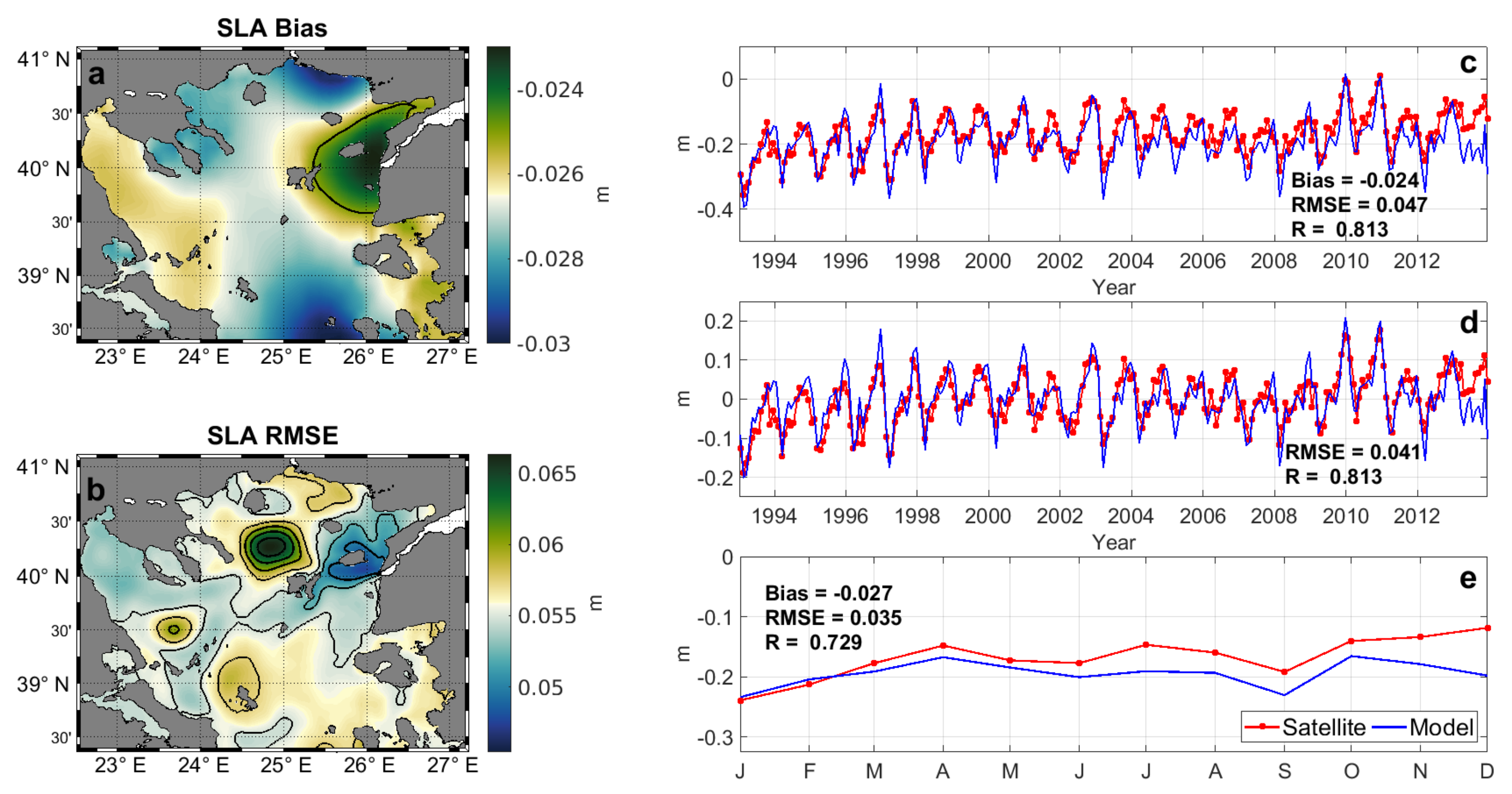
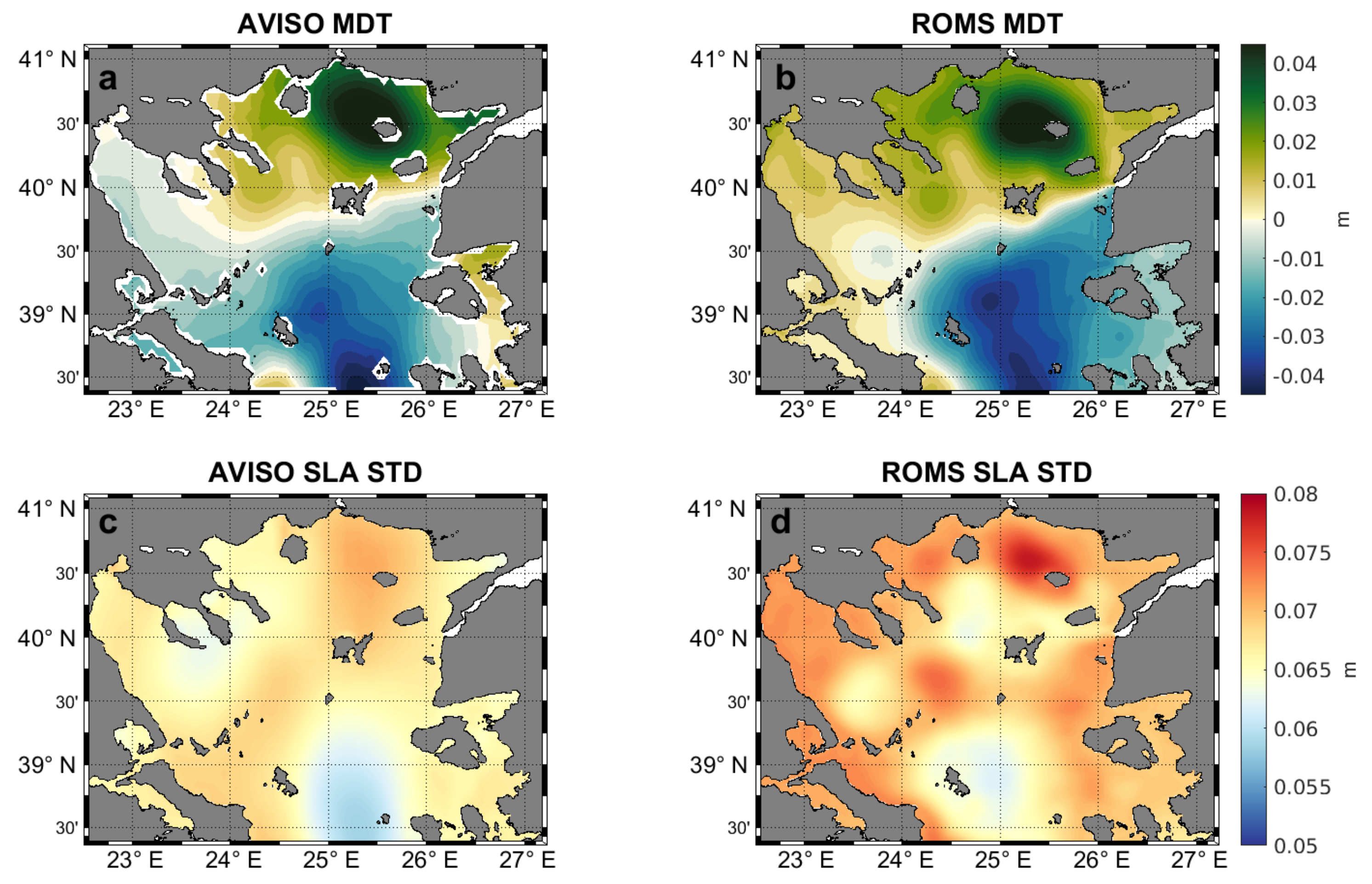
3.1.2. Sea Level Anomaly

The direct comparison of satellite sea level anomalies required the estimation of steric height as a post process, due to the model’s hydrostatic approximation. Although non-Boussinesq steric effects have a negligible imprint on monthly or longer regional sea level patterns, they do impact global mean sea levels [55,56]. The mean sea level of the regional model [57], from which we extracted the boundary conditions, does not include the global mean steric effect. Thus, the steric height component was estimated using a maximum integration depth of 600 m and the Gibbs Seawater (GSW) Oceanographic toolbox [58]. The estimated daily steric height was added to the model’s dynamic height ( ζ ). The results of the sea-level validation are presented in Figure 6 in the form of error maps (Bias and RMSE) and as basin-integrated time series for 21 years.
We also validate our simulation of mean dynamic topography (MDT), which reflects the average strength of geostrophic currents. We used the CMEMS MDT 2020 product which provides an estimate of the mean sea surface height above the geoid on a 4.6 km resolution in both directions horizontally. It is based on altimetry data, in situ measurements of temperature and salinity and covers the period 1992–2012. Figure 7 shows a comparison between simulations and satellite observations, both for the general circulation (as expressed by Mean Dynamic Topography, panels a and b) and its variability (as expressed by the standard deviation of the Sea-Level Anomaly, panels c and d). The Mean Dynamic Topographies are expressed as anomalies with respect to the area-weighted regional mean, as estimated from observations and simulation.
The relatively crude grid-size of satellite altimetry products (1/8 of a degree) results in lower effective resolution compared to our model’s. For that reason, small-scale features in the model results are difficult to evaluate. Moreover, land contamination leads to a lower accuracy of satellite altimetry in coastal regions [59], while corrections for the inverse barometer effect, tides, and high frequency winds [60], in satellite altimetry products lead to reduced accuracy in regions such as the North Aegean Sea, where these corrections are difficult to model.
Comparison of simulated and observed Mean Dynamic Topography reveals that the model reproduces very satisfactorily the anticyclonic flow around Samothraki Island, and the cyclonic circulation south of Lemnos Island (Figure 7a,b). The Sea-Level Anomaly standard deviation maps show highest variability in the area of the Samothraki anticyclone, and least in Skyros basin, with the model exhibiting higher overall variability than the observed values, a fact possibly related to the lower resolution of the satellite data, as discussed above.
Based on our calculations, the model underestimates the sea level by approximately 2 cm (Figure 6a,c) and has an overall error of 4.5 cm. Murphy’s skill score for the full signal is approximately 0.75 and for the de-seasoned 0.76.

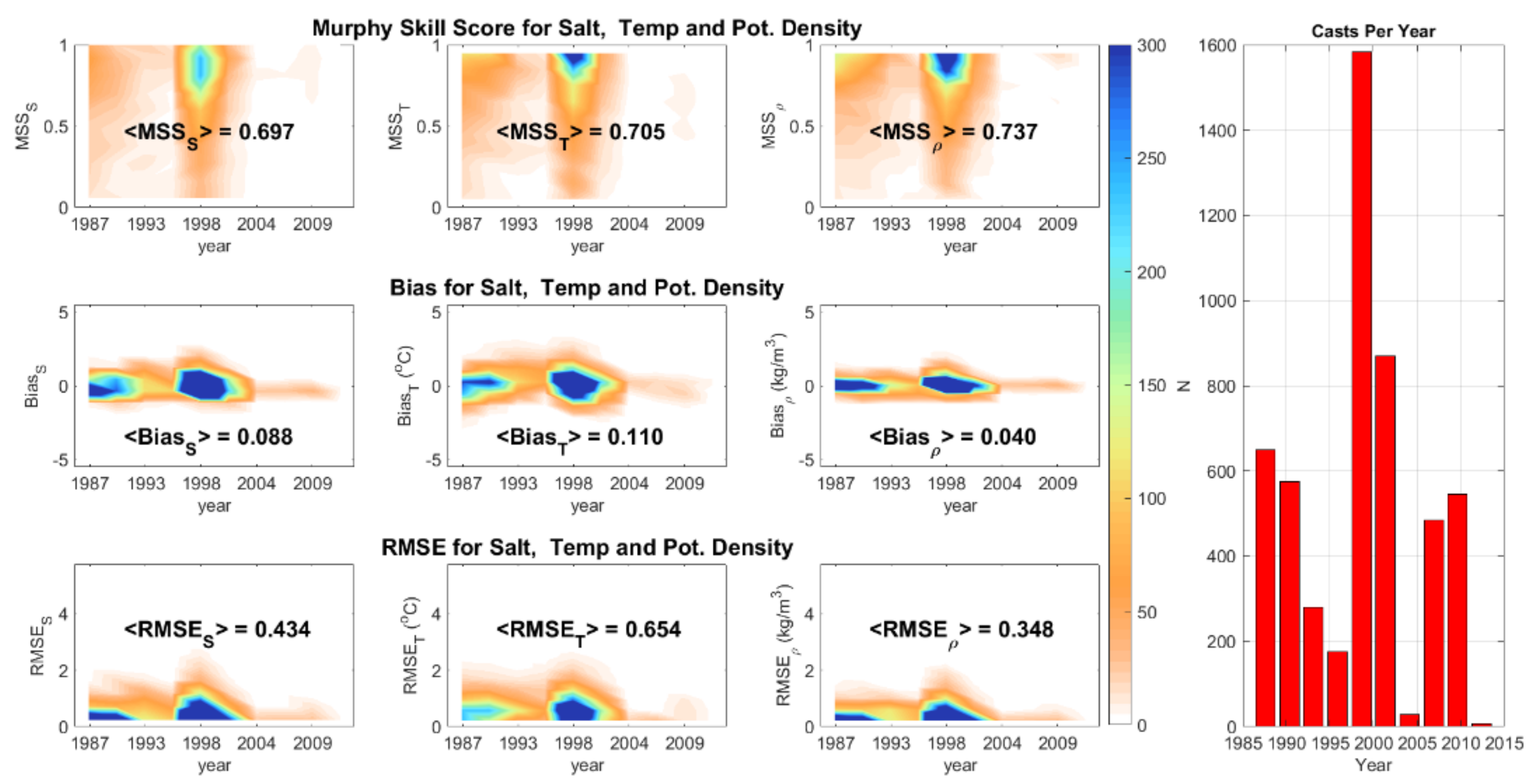
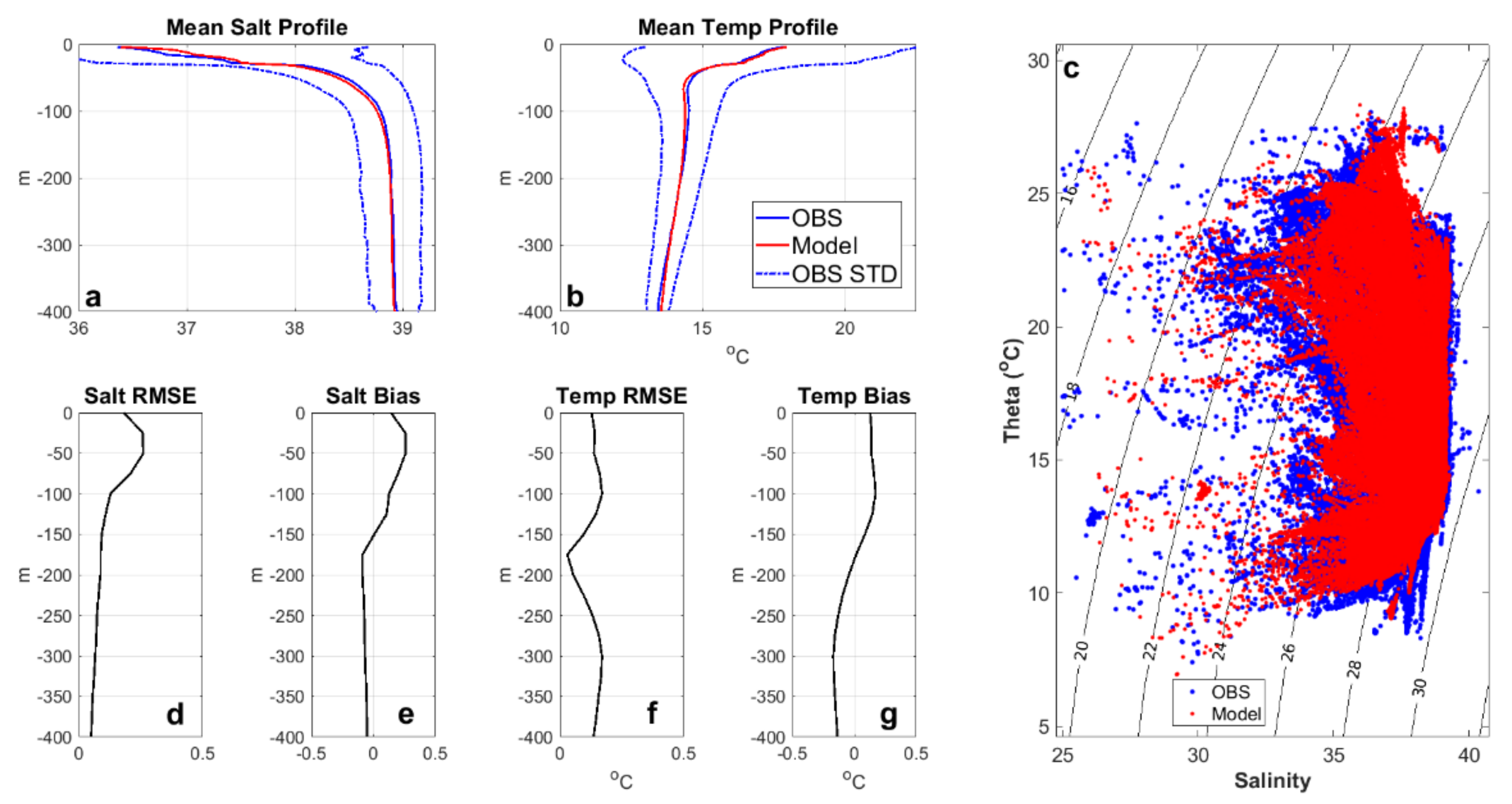
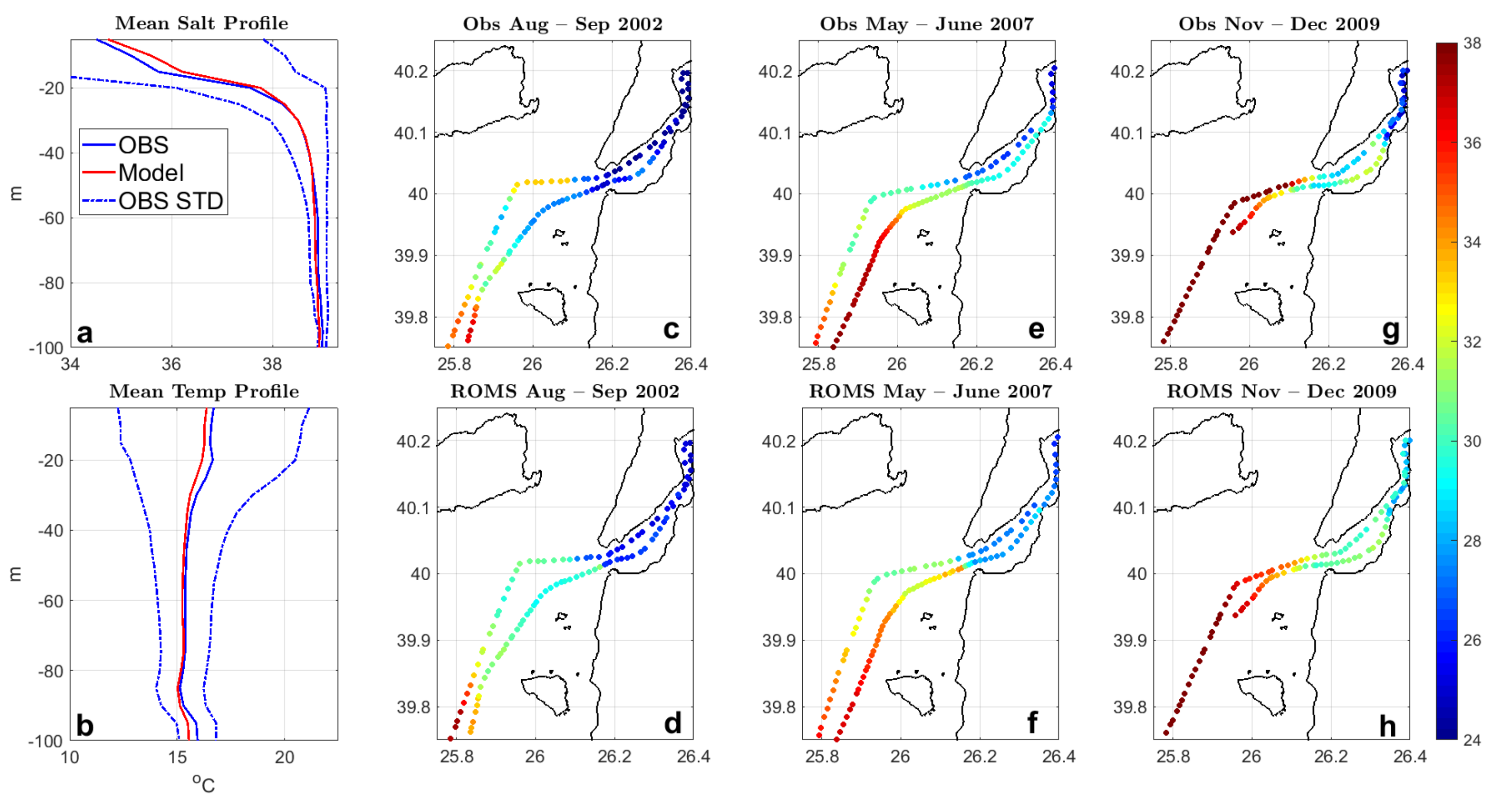
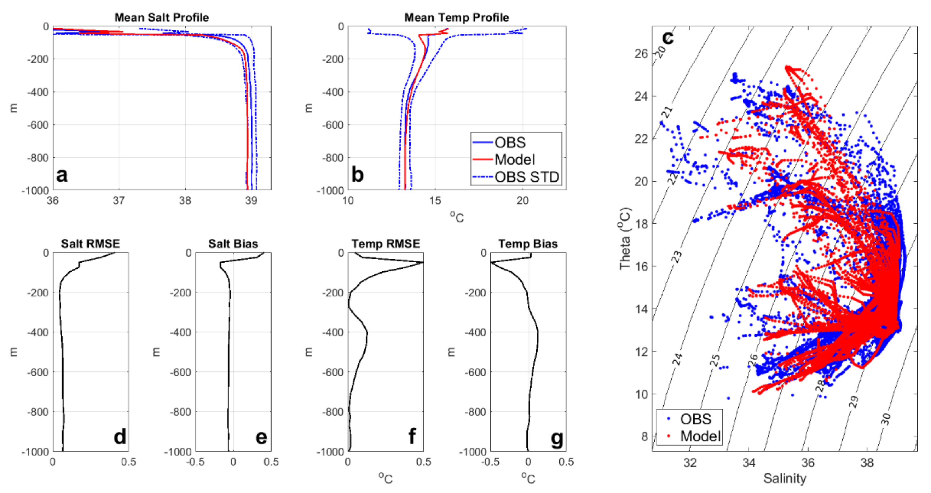
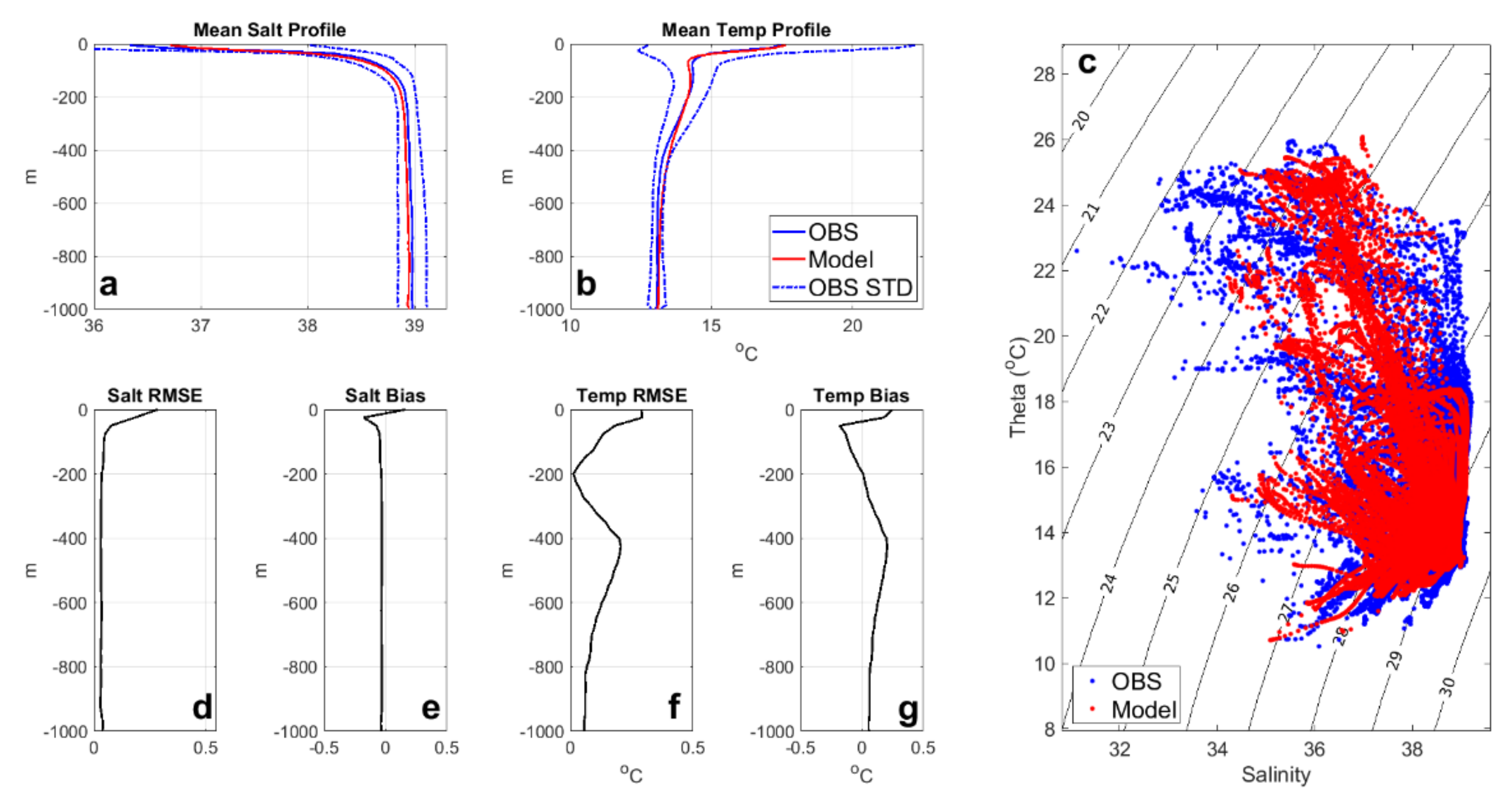
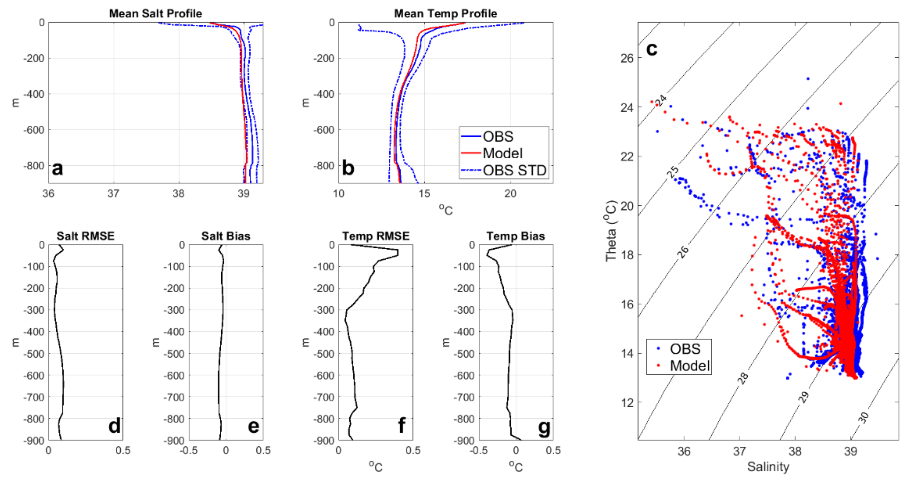
3.1.3. Hydrographic Properties—θ/S Profiles

The most important part of the validation is, in our opinion, the direct comparison of the model’s results with θ/S profiles to evaluate its capability of reproducing the vertical structure and characteristics of the area of interest. The overall model skill for potential temperature, salinity, and potential density from the available casts (mainly R/V CDT data, complemented by XBTs and Bottles) for the period from January 1986 to December 2013, are presented in Figure 8. Positions are shown in Figure 1 and the number of acceptable data—QC flag “good”—is 5119. Unfortunately, only a small proportion of the available profiles—639 casts or 12.5% of the total number of casts—were recorded from the North Aegean’s deep basins, and as seen from the histogram in Figure 8, a significant issue is the temporal inhomogeneity of observations during the last few decades. The vast majority (87.5%) covers depths from the surface to 450 m. A quick and obvious finding from the model performance positive Bias is that it tends to slightly overestimate both salinity and temperature. However, in terms of potential density, the results show the that the model is capable of reproducing the observed water types, having a positive Bias of 0.04 kg/m3 and a good—higher than 0.5—performance index, according to Murphy’s skill score for all fields (T,S,ρ).
A more focused analysis of the hydrographic results for the surface and the intermediate water column is provided in Figure 9. The presented results are the outcome of the comparison between the model’s output and the available θ/S profiles for the period from 1986 to 2013 in terms of hydrographic properties and error estimation. First, the mean profile from all observational data was estimated by averaging in time and space for the full extent of the North Aegean. Model data were interpolated in time (to accurately match the cast time of the observations because we kept only daily means for the prognostic fields of temperature and salinity) and averaged spatially. From the mean observed and modelled profiles, the Bias and the RMSE of the first 400 m were estimated, using a 25 m vertical step. Panels a and b (Figure 9) show the mean salinity and potential temperature profile as calculated from model’s data and observations, as well as an estimate of the observed variation (±one standard deviation). Panels d, e, f, and g give the error estimation expressed using Bias and RMSE for salinity and temperature. Finally, the overall θ/S diagram for all profiles for the upper 400 m for the 28-year-long (panel c) exhibits a very good reproduction of the observed water-masses by the hindcast.
The temperature overestimation extends from the sea-surface (as seen already in Section 3.1.1) to the upper 160–170 m (Figure 9g) having about the same magnitude (0.2 °C) as the SSTs. The Bias reverses sign to negative in the layer below and gradually decreases. This is in agreement with the RMSE vertical distribution (Figure 9f), where the best score—of almost 0.03 °C—is approximately at 180 m, decreasing below 300 m. A possible cause for the temperature positive Bias in the surface layer may be the Jerlov water type selected to replicate the optical properties of the seawater in the North Aegean. After several sensitivity runs, it was set as type 3 in ROMS nomenclature, i.e., IB Western Mediterranean [61], constant for the whole numerical grid.
For the case of salinity, a high RMSE appears at the first 100 m (Figure 9d) and again, as in temperature, a positive Bias for the upper 170 m. Below that depth, both RMSE and Bias gradually decrease until 400 m, where they obtained the best scores. A part of the error comes from the southern open boundary, where data from a Mediterranean regional-scale model were used [33]. According to available quality information documents for the version providing the boundary conditions, the regional-scale model exhibited an overall positive Bias for salinity, notably for the Aegean Sea region. The contribution of the eastern open boundary to the overall salinity error, at first glance, is mainly local, as it mostly affects the Dardanelles exit several kilometres away from it but contributes to the overall salt budget. An analysis for the eastern open boundary behaviour and its effect are shown in Figure 10.
The mean profiles of salinity and temperature are shown in Figure 10 (panels a and b) at the first 100 m in the area directly affected by the Dardanelles straits outflow (denoted by the black dashed-line rectangle at Figure 1). Error in terms of Bias and RMSE is 0.07 and 0.13 for the mean salinity and −0.17 °C and 0.21, respectively, for the mean temperature. For the surface salinity (panels d, f, and h) the mean absolute error is 0.39, 0.42 and 0.45 for 2002, 2007 and 2009, respectively. Here, we must clarify that the salinograph data from all three cruises cover one day per month, 5 August and 11 September 2002, 10 May and 15 June 2007 and finally 1 November and 15 December 2009, have a high temporal resolution—6 min—and are compared with an interpolated in time daily average salinity field. The use of the data of Maderich et al. [20] for the eastern open boundary of our computational grid offered not only locally, as presented at Figure 10a,b, but overall (for both surface and the upper layers of intermediate waters, Figure 9) reasonable results concerning the characteristics/properties of the Black Sea waters that enter the North Aegean through Dardanelles straits.
Another contribution to the salinity positive Bias comes from the riverine contribution in the North Aegean Sea. The riverine importance in terms of nutrient load, as well as the thermohaline functioning of the area, is extensively discussed by Tsiaras et al. [62]. In our case, the lack of salinity data in the river outflow time series from E-HYPE forced us to use a constant value for the simulation. After several test runs, we set the salinity value equal to 14 in order to obtain stable solutions and mainly to remove unrealistic freshwater surface fronts with sharp vertical gradients at the first 10 m in the coastal areas close to the rivers exit. Numerical stability was eventually achieved, but with the aforementioned cost potentially added to the total salinity error.
The second part of our analysis for the θ/S profiles is focused on the deep basins of the North Aegean Sea and their variability. We have extensively compared the available hydrographic data for each of the basins with the model’s output and the final results are presented at the following figures (Figure 11, Figure 12 and Figure 13). Lemnos basin (Figure 1 cyan rectangular) is an oblong basin with a mean depth of approximately 500 m at the northeast part of the North Aegean. The deepest part is 1582 m and is located north of the island of Lemnos. The number of θ and S profiles is 184 but with significant temporal inconsistencies. Figure 11 shows the mean salinity and temperature profile from the surface to 1000 m depth and its errors estimation plus a θ/S diagram. The mean profiles were calculated with the same approach as described previously for surface and the intermediate depths.
The θ/S diagram (panel c) of the above figure exhibits a realistic representation of the Lemnos basin water mass structure, especially for the deeper-than-400 m layers. The mean simulated salinity profile is within one standard deviation of the observed (panel a), while the corresponding temperature profile is very close to observations (panel b). The model slightly underestimates salinity, with an almost constant with depth error (panels c and e). A similar picture is seen for temperature, with a decreasing error as we go deeper in the water column (panels f and g). The maximum error for both tracers is found in the upper surface layers. For temperature, although the overall Bias has a positive sign (0.16 °C), from the surface to a depth of approximately 60 m it becomes negative with the maximum absolute value for Bias to be equal to 0.32 °C. From that depth and below, Bias and RMSE gradually decrease until the depth of 250 m. The maximum positive Bias is found at the 400 m and is equal to 0.1 °C.
Figure 12 shows the hydrographic characteristics of the Athos basin (Figure 1 blue rectangle) for the upper 1000 m (maximum depth 1561 m), where the number of the available observations is almost twice that of the Lemnos basin. The mean profiles (panels a and b) and the θ/S diagram (panel c) reveal the model’s capability for this basin also its ability to replicate, in a realistic way, the structure of the water column from the surface to the deepest point. The errors for temperature and salinity (panels d–g) are smaller compared to north Lemnos basin and exhibit the same behaviour. An interesting finding is salinity’s Bias value below 200 m, which is constant and even smaller than the north Lemnos basin, with a value equal to −0.019. Summarizing for the Athos basin, it can be concluded that the model has a very good performance in this part of the North Aegean.
The results for the north Skyros basin are shown at Figure 13. The number of available θ/S profiles was smaller than for the other basins (133) and had the biggest temporal gaps. The maximum depth of the basin is 1091 m. Both parameters exhibit a negative Bias which is almost constant for salinity and variable for the upper 400 m for temperature. The highest undershot is located in the 50 m where the RMSE is 0.32 °C and Bias −0.29 °C. As seen in the previous figures, the error is reduced below 400 m. Again, the agreement of the water masses in the θ/S diagram is acceptable as for the other two basins, despite the relative scarcity of observations.
As the validation results point to a very good performance of the model in the deep layers, which are considered the “clearest” recorders of climatic variability, it is possible to analyse the evolution of the deep layers, expressed through the interannual variability of potential density ( σ θ 0 ), integrated from 600 m to the maximum depth of its basin with a daily step (Figure 14). The major deep-water formation events that happened during the late 1980s and early 1990s—1987, 1992 and 1993—known as the EMT, are seen in the time series presented along with other (smaller in magnitude) events that took place during the simulated 28-year period.
One more argument about the validity of the simulated results is provided in Figure 15, where the interannual variability of the north Aegean deep basins’ potential density from the available observations is compared with the model output, integrated vertically below 600 m. The Bias sign in the three basins reveals that the model slightly underestimates the density of the deep waters. The total error (RMSE) is exceptionally small for the time span of the simulation.
The overall scores of the simulation show that the model’s error is in an acceptable range for a free run and even comparable/adequate with an assimilative one [63]. Notably, the model underestimates the density of the deep-layer waters produced in the EMT period (1987–1993), however it reproduces well the rate at which the density of the deep layers progressively decays in the three layers.

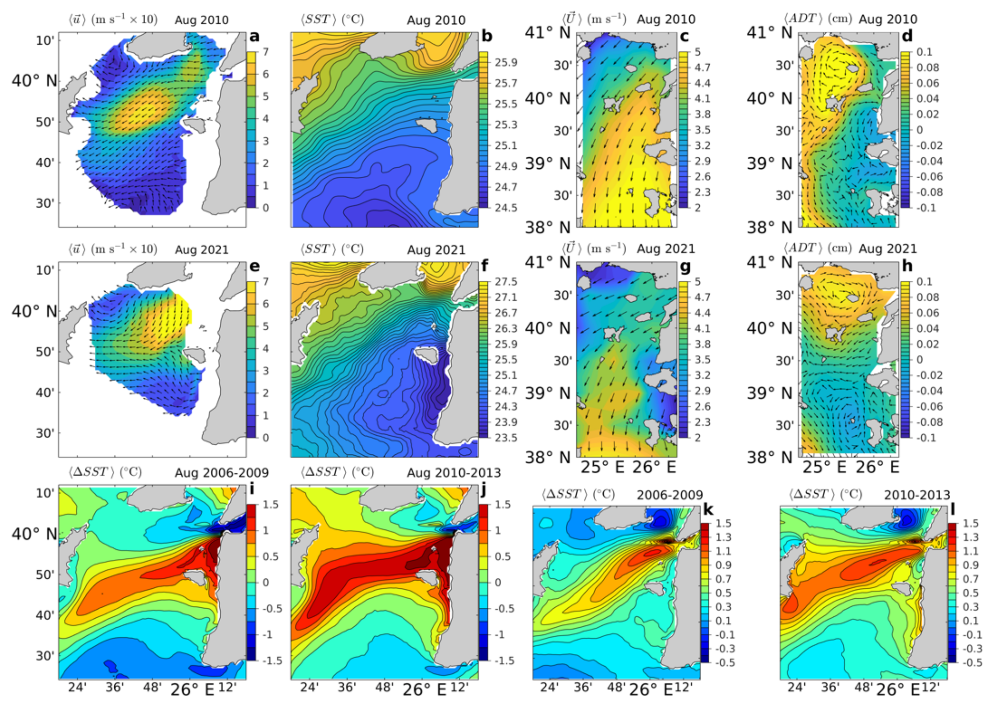
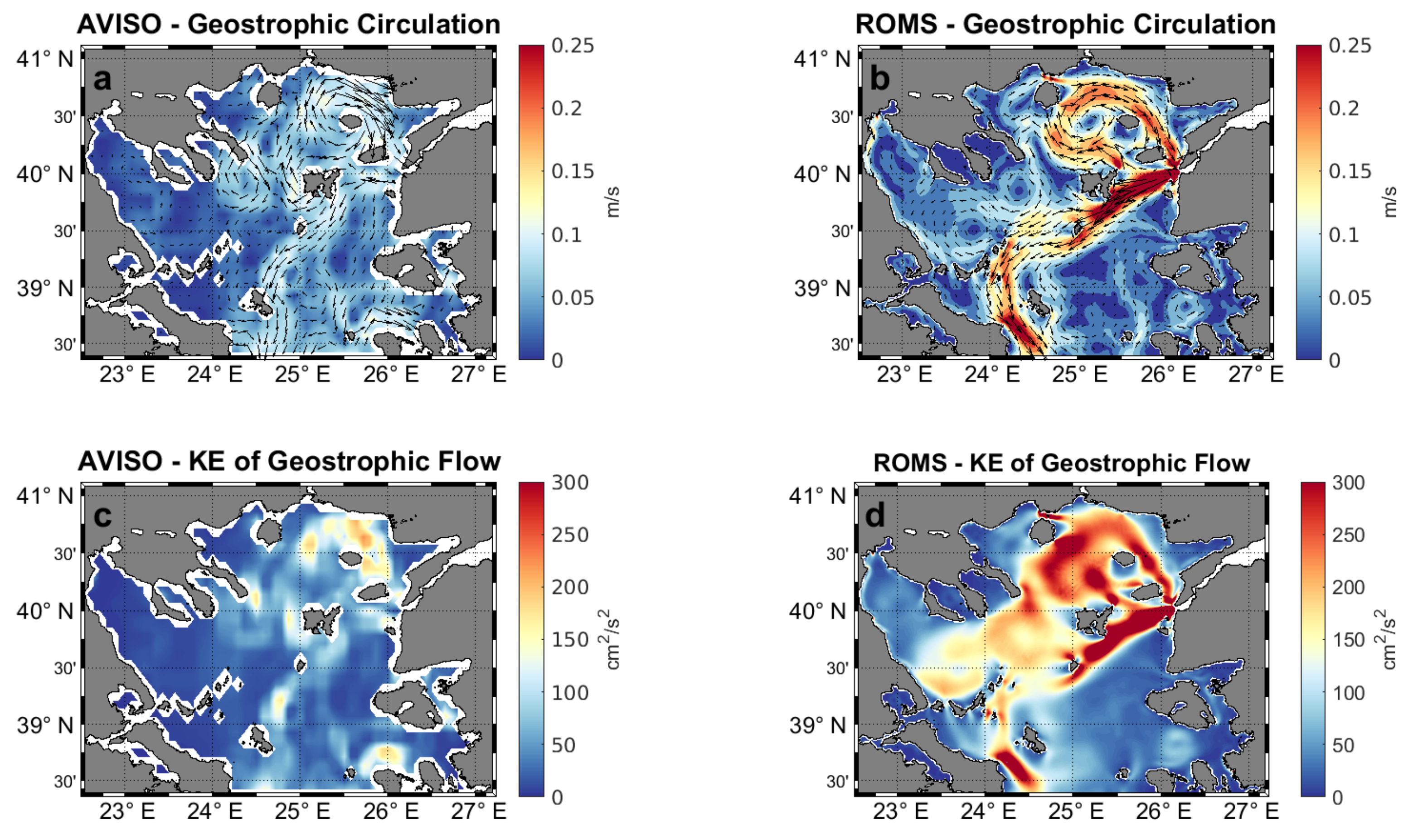
3.1.4. Surface Circulation

Regarding the surface circulation, the model reproduces to a high degree the general pattern, as described from previous works [18], and is in agreement with the satellite observations [64]. In the northern part of the domain (Figure 16b), the most prominent feature is the distinct pathway of the Black Sea waters that enter the North Aegean Sea through the Dardanelles and split east of Lemnos Island creating two branches, one going to the northern part and contributing to the Samothrace eddy. The second branch initially follows a south-westward route to the central Aegean through the Evia island jet and later westwards forming the Chios cyclone. Regarding the geostrophic kinetic energy distribution, the highest energy levels for the model (Figure 16d) are located mainly south of Lemnos Island and at the north-eastern part of the domain, in the region between the islands of Thasos, Samothrace and Lemnos, where an anticyclonic system dominates the local circulation.
Consequently, the observed highest kinetic energy is found at the same areas but with a smaller magnitude. An interesting finding is the low signal of the Sporades eddies in the satellite data results (Figure 16c). In both cases, the differences in magnitude have to do with the higher spatial resolution of the model (1 km) compared to the original satellite information (1/8 of a degree). Due to the low resolution of the observed sea-level fields, the high-wavenumber part of the spatial two-dimensional spectrum does not contribute to the total variance, which explains the mismatch.
Another validation of the model’s ability to reproduce the surface circulation can be provided by the presence of the HF radar system “DARDANOS” covering the wider area of the Dardanelles outflow in the northeast Aegean [46]. The validation is held via comparison of the seasonal surface circulation at the Dardanelles strait exit for 2010, as derived from HF radar data and the model. The radar’s reconstructed data have 30 min temporal resolution and 0.5 km spatial resolution. To compare them with the model’s results, daily mean fields are calculated and interpolated linearly to match the model’s resolution. Overall, the model reproduces well the local circulation (Figure 17). The model has an error pattern similar to that of the seasonal sea surface temperature (Figure 3). The maximum deviation takes place during the winter months (January, February and March) and then gradually reduces as time evolves. A possible explanation beyond the parameterization applied for the Dardanelles outflow after 2009 (a climatological mean year from the period 1985 to 2009), can be the low spatial resolution of the wind field input forcing the simulation. This, combined with outflow mismatches due to the parameterization, may be the source of the observed deviations.

4. Discussion

A new model has been developed for the Aegean Sea, based on the ROMS platform, suitably configured to enable climatological studies of the basin. The replacement of seasonal-cycle parameterizations of the exchanges with the Black Sea by time-dependent fluxes, as determined by Maderich et al. [20], as well as the removal of all climatological relaxation terms from the numerical schemes, enables the simulation of changing climatic conditions. An evaluation of the model performance through the comparison of the 30-year-long hindcast to all available oceanographic information revealed that the model, despite the removal of relaxation terms and the lack of data assimilation, exhibits very small Bias and RMSE, and, especially important for long-term simulations, shows no sign of significant numerical drift (as far as can be deduced from the available observations). Furthermore, the model satisfactorily reproduces the surface circulation of the North Aegean Sea, both on a large scale (i.e., the whole basin) as well as over the critical region of the vicinity of the Dardanelles exit. Thus, the model provided a well-validated 30-year-long hindcast (1985–2015) of the hydrodynamics of the Aegean Sea, suitable for a range of further studies. Of special interest is that the model exhibits its best performance in the deep basins of the North Aegean Sea, repositories of climatic variability information, shedding light on the evolution of the deep layers throughout the whole hindcasting period.
Moreover, the model hereby introduced exhibits very good performance, with small biases in the temperature and salinity profiles. Potential sources of the salinity Bias, such as the lateral boundary conditions and the riverine inputs, have already been discussed. An open question is the net E-P contribution, as estimated from the COARE [38] bulk formulae using ERA5 input (for the total accumulated precipitation and radiative fluxes). The question is raised from the known issues that previous ERA datasets (ERA 40 and Interim) had in the overall rainfall rates globally and fluxes locally in the Mediterranean Sea [65,66]. Although the ERA5 model is significantly improved in total and over the global ocean, we do not have any knowledge from the available bibliography for its skill over the Mediterranean Sea and how it may impact the overall E-P-R budget.
Regarding the reproduction of the sea-level, the skill score index of our model results is lower compared to the SSTs score. However, the model adequately reproduces the seasonal, inter and intra-annual variability, and some of the deviation between the simulated and observed sea level should be attributed, in our opinion (and according to the available literature), to the temporal variability of the mass component of sea level (contribution from meltwater and salt, [67]). A noteworthy fact is that the model reproduces the large positive sea-level anomalies in 2010 and 2011, which is in agreement with findings by Landerer and Volkov [68] during the same period in the Mediterranean Sea.
The hereby produced 30-year hindcast, exhibiting the least Bias in the deep layers, fills the observational gaps in the evolution of the deep basins (Figure 14 and Figure 15). Based on the slopes of the density time-series, three significantly different periods can be identified: The short and episodic dense-water formation events (namely in the winters of 1987, 1992, 1993 and smaller episodes in 2008 and 2012, and a gradual increase of density after 2008), the periods of stagnation (characterized by decreasing densities), and the steady-state periods (where the density remains more of less constant). The periods of stagnation correspond to a dynamical balance between the rate of buoyancy gain in the deep basin and the downward vertical buoyancy flux through the interface between intermediate and deep waters [69,70]. The periods of steady state usually take place after prolonged stagnation periods have led to gradual homogeneity between the intermediate and deep layers, and, thus, the turbulent fluxes across the boundary are minimal. Based on this work’s result, which has filled gaps in the observational record due to lack of frequent of CTD casts, the most distinctive stagnation period in the North Aegean deep basins followed the EMT and lasted until about 2004, while the period between 2004 and 2008 can be characterized as a steady-state period.
Overall, north Skyros basin appears more sensitive to buoyancy forcing, exhibiting higher overall density variability and direct deep-water formation in the winters of 2006, 2008 and 2012, while the deep layers of Athos exhibit a gradual density increase, suggestive of a slow replenishment mechanism through lateral exchanges with neighbouring basins, possibly the Skyros basin.
Thus, the hereby introduced model is suitable for high-resolution climatological studies of the Aegean Sea. The high resolution of the numerical domain enables the full simulation of mesoscale geostrophic circulation, as well as the simulation of tidal propagation and the dynamics of the low-wavenumber part of the internal-wave spectrum. Despite the fact that the hereby-presented hindcast exhibits acceptable deviation from the observed Aegean Sea hydrographic properties and variability, the model set-up permits the planning and execution of more advanced numerical experiments, incorporating astronomical forcing, and thus simulating high-frequency processes, such as the generation, propagation and dissipation of internal baroclinic tides, the energy exchange between tidal frequencies and the internal-wave continuum, and the energy flow towards turbulence and mixing. Furthermore, the success of the simulation of the above small-scale processes can be assessed (as compared to the “basic” hindcast hereby presented) based on the same methodology and observations used in this work.

Author Contributions

Conceptualization, E.T. and V.Z.; methodology, E.T., V.Z. and I.G.M.; software, I.G.M.; numerical modelling, I.G.M.; validation, I.G.M. and E.P.; formal analysis, I.G.M., E.P. and V.Z.; investigation, I.G.M. and E.T.; data curation, I.G.M.; writing—original draft preparation, I.G.M., V.Z., E.P. and E.T.; writing—review and editing, I.G.M., V.Z., E.P., E.T. and S.P.; supervision, E.T. and V.Z.; project administration, E.T. and V.Z.; funding acquisition, V.Z. All authors have read and agreed to the published version of the manuscript.

Funding

This work has been supported by the Policy-oriented marine Environmental Research for the Southern European Seas (PERSEUS) funded by the EU under FP7 Theme “Oceans of Tomorrow” OCEAN.2011-3, Grant Agreement No. 287600. This work was also partially supported by the project “Hellenic Integrated Marine Inland water Observing, Forecasting and Offshore Technology System (HIMIOFoTS)”, implemented in the framework of Operational Programme Competitiveness, Entrepreneurship and Innovation 2014–2020 (EPAnEK) (MIS 5002739), cofunded by the European Union through the European Regional Development Fund and the Hellenic State through ESPA 2014–2020.

Data Availability Statement

The data presented in this study are available on request from the corresponding author.

Acknowledgments

We are grateful to Nadia Pinardi for her support, advice and the provision of the necessary data from their initial reanalysis dataset of the Mediterranean Sea for our model setup and hindcast. The Ssalto/Duacs altimeter products were produced and distributed by the Copernicus Marine and Environment Monitoring Service (CMES) (https://marine.copernicus.eu/, accessed on 1 September 2021). The numerical simulations were performed in the national HPC facility—ARIS—of the Greek Research and Technology Network (GRNET) under the projects ID pr001041 (1st Pilot call) named PALIROIA and pr006058 (6th call) named TWIK.

Conflicts of Interest

The authors declare no conflict of interest. The funders had no role in the design of the study; in the collection, analyses, or interpretation of data; in the writing of the manuscript, or in the decision to publish the results.

References

  1. Nielsen, J.N. Hydrography of the Mediterranean and adjacent waters. In Report of the Danish Oceanographic Expeditions 1908–1910 to the Mediterranean and Adjacent Seas; Schmidt, J., Ed.; Andr. Høst and Søn: Copenhagen, Denmark, 1912; pp. 77–192. [Google Scholar]
  2. Gertman, I.; Pinardi, N.; Popov, Y.; Hecht, A. Aegean Sea Water Masses during the Early Stages of the Eastern Mediterranean Climatic Transient (1988–90). J. Phys. Oceanogr. 2006, 36, 1841–1859. [Google Scholar] [CrossRef]
  3. Tragou, E.; Petalas, S.; Mamoutos, I. Air-Sea Interaction—Heat and freshwater fluxes in the Aegean Sea. In The Aegean Sea Environment: The Natural System; Barcelo, D., Kostianoy, A.G., Eds.; The Handbook of Environmental Chemistry; Springer: Berlin/Heidelberg, Germany, 2021; Chapter A-10; Accepted for publication. [Google Scholar]
  4. Zervakis, V.; Georgopoulos, D.; Drakopoulos, P.G. The role of the North Aegean in triggering the recent Eastern Mediterranean climatic changes. J. Geophys. Res. Ocean. 2000, 105, 26103–26116. [Google Scholar] [CrossRef]
  5. Roether, W.; Klein, B.; Manca, B.B.; Theocharis, A.; Kioroglou, S. Transient eastern Mediterranean deep waters in response to the massive dense-water output of the Aegean Sea in the 1990s. Prog. Oceanogr. 2007, 74, 540–571. [Google Scholar] [CrossRef]
  6. Tzali, M.; Sofianos, S.; Mantziafou, A.; Skliris, N. Modelling the impact of Black Sea water inflow on the North Aegean Sea hydrodynamics. Ocean. Dyn. 2010, 60, 585–596. [Google Scholar] [CrossRef]
  7. Ignatiades, L.; Psarra, S.; Zervakis, V.; Pagou, K.; Souvermezoglou, E.; Assimakopoulou, G.; Gotsis-Skretas, O. Phytoplankton size-based dynamics in the Aegean Sea (Eastern Mediterranean). J. Mar. Syst. 2002, 36, 11–28. [Google Scholar] [CrossRef]
  8. Zervoudaki, S.; Nielsen, T.G.; Christou, E.D.; Siokou-Frangou, I. Zooplankton distribution and diversity in a frontal area of the Aegean Sea. Mar. Biol. Res. 2006, 2, 149–168. [Google Scholar] [CrossRef]
  9. Siokou-Frangou, I.; Zerviudaki, S.; Christou, E.D.; Zervakis, V.; Georgopoulos, D. Variability of mesozooplankton spatial distribution in the North Aegean Sea, as influenced by the Black Sea water outflow. J. Mar. Syst. 2009, 78, 557–575. [Google Scholar] [CrossRef]
  10. Maina, I.; Kavadas, S.; Katsanevakis, S.; Somarakis, S.; Tserpes, G.; Georgakarakos, S. A methodological approach to identify fishing grounds: A case study on Greek trawlers. Fish. Res. 2016, 183, 326–339. [Google Scholar] [CrossRef]
  11. Korres, G.; Lascaratos, A.; Hatziapostolou, E.; Katsafados, P. Towards an Ocean Forecasting System for the Aegean Sea. J. Oper. Oceanogr. 2002, 8, 191–218. [Google Scholar] [CrossRef]
  12. Korres, G.; Nittis, K.; Perivoliotis, L.; Tsiaras, K.; Papadopoulos, A.; Triantafyllou, G.; Hoteit, I. Forecasting the Aegean Sea hydrodynamics within the POSEIDON-II operational system. J. Oper. Oceanogr. 2010, 3, 37–49. [Google Scholar] [CrossRef]
  13. Nittis, K.; Zervakis, V.; Perivoliotis, L.; Papadopoulos, A.; Chronis, G. Operational Monitoring and Forecasting in the Aegean Sea: System Limitations and Forecasting Skill Evaluation. Mar. Pollut. Bull. 2001, 43, 154–163. [Google Scholar] [CrossRef] [PubMed]
  14. Nittis, K.; Perivoliotis, L.; Korres, G.; Tziavos, C.; Thanos, I. Operational monitoring and forecasting for marine environmental applications in the Aegean Sea. Environ. Model. Softw. 2006, 21, 243–257. [Google Scholar] [CrossRef]
  15. Kourafalou, V.H.; Barbopoulos, K. High resolution simulations on the North Aegean Sea seasonal circulation. Ann. Geophys. 2003, 21, 251–265. [Google Scholar] [CrossRef] [Green Version]
  16. Vervatis, V.; Skliris, N.; Sofianos, S. INTER-annual/decadal variability of the north Aegean Sea hydrodynamics over 1960–2000. Mediterr. Mar. Sci. 2014, 15, 696–705. [Google Scholar] [CrossRef] [Green Version]
  17. Vervatis, V.D.; Sofianos, S.; Skliris, N.; Somot, S.; Lascaratos, A.; Rixen, M. Mechanisms Controlling the Thermohaline Circulation Pattern Variability in the Aegean-Levantine Region. A Hindcast Simulation (1960–2000) with an Eddy Resolving Model. Deep Sea Res. Part I Oceanogr. Res. Pap. 2013, 74, 82–97. [Google Scholar] [CrossRef]
  18. Androulidakis, Y.S.; Krestenitis, Y.N.; Kourafalou, V.H. Connectivity of North Aegean circulation to the Black Sea water budget. Cont. Shelf Res. 2012, 48, 8–26. [Google Scholar] [CrossRef]
  19. Mavropoulou, A.M.; Mantziafou, A.; Jarosz, E.; Sofianos, S. The influence of Black Sea Water inflow and its synoptic time-scale variability in the North Aegean Sea hydrodynamics. Ocean. Dyn. 2016, 66, 195–206. [Google Scholar] [CrossRef]
  20. Maderich, V.; Ilyin, Y.; Lemeshko, E. Seasonal and interannual variability of the water exchange in the Turkish Straits System estimated by modelling. Mediterr. Mar. Sci. 2015, 16, 444–459. [Google Scholar] [CrossRef] [Green Version]
  21. Shchepetkin, A.F.; McWilliams, J.C. A method for computing horizontal pressure-gradient force in an oceanic model with a nonaligned vertical coordinate. J. Geophys. Res. 2003, 108, 3. [Google Scholar] [CrossRef]
  22. Shchepetkin, A.F.; McWilliams, J.C. The regional oceanic modeling system (ROMS): A split-explicit, free-surface, topography-following-coordinate oceanic model. Ocean Model. 2005, 9, 347–404. [Google Scholar] [CrossRef]
  23. Sikirić, M.D.; Janeković, I.; Kuzmić, M. A new approach to bathymetry smoothing in sigma coordinate ocean models. Ocean Model. 2009, 29, 128–136. [Google Scholar] [CrossRef]
  24. Beckmann, A.; Haidvogel, D.B. Numerical Simulation of Flow around a Tall Isolated Seamount. Part I: Problem Formulation and Model Accuracy. J. Phys. Oceanogr. 1993, 23, 1736–1753. [Google Scholar] [CrossRef] [Green Version]
  25. Haney, R.L. On the Pressure Gradient Force over Steep Topography in Sigma Coordinate Ocean Models. J. Phys. Oceanogr. 1991, 21, 610–619. [Google Scholar] [CrossRef] [Green Version]
  26. Marchesiello, P.; Debreu, L.; Couvelard, X. Spurious diapycnal mixing in terrain-following coordinate models: The problem and a solution. Ocean Model. 2009, 26, 156–169. [Google Scholar] [CrossRef]
  27. Holland, W.R.; Chow, J.C.; Bryan, F.O. Application of a third-order upwind scheme in the ncar ocean model. J. Clim. 1998, 11, 1487–1493. [Google Scholar] [CrossRef]
  28. Webb, D.J.; De Cuevas, B.A.; Richmond, C.S. Improved advection schemes for ocean models. J. Atmos. Ocean. Technol. 1998, 15, 1171–1187. [Google Scholar] [CrossRef]
  29. Smolarkiewicz, P.K.; Margolin, L.G. MPDATA: A finite-difference solver for geophysical flows. J. Comput. Phys. 1998, 140, 459–480. [Google Scholar] [CrossRef] [Green Version]
  30. Mellor, G.L.; Yamada, T. Development of a turbulence closure model for geophysical fluid problems. Rev. Geophys. 1982, 20, 851–875. [Google Scholar] [CrossRef] [Green Version]
  31. Iona, A.; Theodorou, A.; Watelet, S.; Troupin, C.; Beckers, J.M.; Simoncelli, S. Mediterranean sea hydrographic atlas: Towards optimal data analysis by including time-dependent statistical parameters. Earth Syst. Sci. Data 2018, 10, 1281–1300. [Google Scholar] [CrossRef] [Green Version]
  32. Hersbach, H.; Bell, B.; Berrisford, P.; Hirahara, S.; Hornyi, A.; Muoz-Sabater, J.; Nicolas, J.; Peubey, C.; Radu, R.; Schepers, D.; et al. The era5 global reanalysis. Q. J. R. Meteorol. Soc. 2020, 146, 1999–2049. [Google Scholar] [CrossRef]
  33. Simoncelli, S.; Fratianni, C.; Pinardi, N.; Grandi, A.; Drudi, M.; Oddo, P.; Dobricic, S. Mediterranean sea physical reanalysis (cmems med-physics). Copernic. Monit. Environ. Mar. Serv. 2019. [Google Scholar] [CrossRef]
  34. Marchesiello, P.; McWilliams, J.C.; Shchepetkin, A. Open boundary conditions for long term integration of regional oceanic models. Ocean Model. 2001, 3, 1–20. [Google Scholar] [CrossRef]
  35. Chapman, D.C. Numerical treatment of cross-shelf open boundaries in a barotropic coastal ocean model. J. Phys. Oceanogr. 1985, 15, 1060–1075. [Google Scholar] [CrossRef] [Green Version]
  36. Flather, R.A. A tidal model of the northwest European continental shelf. Mem. Soc. R. Sci. Liege 1976, 10, 141–164. [Google Scholar] [CrossRef]
  37. Lindstrom, G.; Pers, C.; Rosberg, J.; Strmqvist, J.; Arheimer, B. Development and testing of the HYPE (Hydrological Predictions for the Environment) water quality model for different spatial scales. Hydrol. Res. 2010, 41, 295–319. [Google Scholar] [CrossRef]
  38. Fairall, C.W.; Bradley, E.F.; Rogers, D.P.; Edson, J.B.; Young, G.S. Bulk parameterization of air-sea fluxes for tropical ocean-global atmosphere coupled-ocean atmosphere response experiment. J. Geophys. Res. 1996, 101, 3747–3764. [Google Scholar] [CrossRef]
  39. Merchant, C.J.; Emburry, O.; Bulgin, C.E.; Block, T.; Corlett, G.K.; Fiedler, E.; Good, S.A.; Mittaz, J.; Rayner, N.A.; Berry, D.; et al. Satellite-based time-series of sea-surface temperature since 1981 for climate applications. Sci. Data 2019, 6, 223. [Google Scholar] [CrossRef] [PubMed] [Green Version]
  40. Nardelli, B.; Tronconi, C.; Pisano, A.; Santoleri, R. High and Ultra-High resolution processing of satellite Sea Surface Temperature data over Southern European Seas in the framework of MyOcean project. Remote Sens. Environ. 2013, 129, 1–16. [Google Scholar] [CrossRef]
  41. Simoncelli, S.; Schaap, D.; Schlitzer, R. Mediterranean Sea—Temperature and salinity Historical Data Collection SeaDataCloud V2, 2020. Available online: https://www.cmcc.it/mediterranean-sea-physical-reanalysis-cmems-med-physics (accessed on 1 September 2021).
  42. Murphy Allan, H. Skill scores based on the mean square error and their relationships to the correlation coefficient. Mon. Weather Rev. 1988, 116, 2417–2424. [Google Scholar] [CrossRef]
  43. Kanarska, Y.; Maderich, V. Modelling of seasonal exchange flows through the Dardanelles Strait. Estuar. Coast. Shelf Sci. 2008, 79, 449–458. [Google Scholar] [CrossRef]
  44. Zodiatis, G.; Balopoulos, E. Structure and characteristics of fronts in the north Aegean Sea. Bollettino Oceanologia Teorica Applicata 1993, 11, 113–124. [Google Scholar]
  45. Zervakis, V.; Kokkini, Z.; Potiris, E. Estimating mixed layer depth with the use of a coastal high-frequency radar. Cont. Shelf Res. 2017, 149, 4–16. [Google Scholar] [CrossRef]
  46. Sylaios, G. Meteorological influences on the surface hydrographic patterns of the North Aegean Sea. Oceanologia 2011, 53, 57–80. [Google Scholar] [CrossRef] [Green Version]
  47. Kokkini, Z.; Potiris, M.; Kalampokis, A.; Zervakis, V. HF Radar observations of the Dardanelles outflow current in North Eastern Aegean using validated WERA HF radar data. Mediterr. Mar. Sci. 2014, 15, 753–768. [Google Scholar] [CrossRef] [Green Version]
  48. Zervakis, V.; Karageorgis, A.P.; Kontoyiannis, H.; Papadopoulos, V.; Lykousis, V. Hydrology, Circulation and distribution of particular matter in Thermaikos Gulf (NW Aegean Sea), during September 2001–October 2001 and February 2002. Cont. Shelf Res. 2005, 25, 2332–2349. [Google Scholar] [CrossRef]
  49. Poulos, S.; Drakopoulos, P.; Collins, M. Seasonal variability in sea surface oceanographic conditions in the Aegean Sea (Eastern Mediterranean): An overview. J. Mar. Syst. 1997, 13, 225–244. [Google Scholar] [CrossRef]
  50. Androulidakis, Y.S.; Krestenitis, Y.N.; Psarra, S. Coastal upwelling over the North Aegean Sea: Observations and simulations. Cont. Shelf Res. 2017, 149, 32–51. [Google Scholar] [CrossRef]
  51. Chaniotaki, M.; Kolovoyiannis, V.; Tragou, E.; Herold, L.A.; Batjakas, I.E.; Zervakis, V. Investigation of the response of the Aegean Sea to the Etesian wind forcing. Cont. Shelf Res. 2021, 225, 104485. [Google Scholar] [CrossRef]
  52. Ciappa, A.C. The summer upwelling of the Eastern Aegean Sea detected from MODIS SST scenes from 2003 to 2015. Int. J. Remote Sens. 2019, 40, 3105–3117. [Google Scholar] [CrossRef]
  53. Demirov, E.; Pinardi, N. Simulation of the Mediterranean Sea circulation from 1979 to 1993: Part, I. The interannual variability. J. Mar. Syst. 2002, 33–34, 23–50. [Google Scholar] [CrossRef]
  54. Mamoutos, I.; Zervakis, V.; Tragou, M.; Karydis, M.; Frangoulis, C.; Kolovoyiannis, V.; Georgopoulos, D.; Psarra, S. The role of wind-forced coastal upwelling on the thermohaline functioning of the North Aegean Sea. Cont. Shelf Res. 2017, 149, 52–68. [Google Scholar] [CrossRef]
  55. Greatbatch, J. A note on the representation of steric sea level in models that conserve volume rather than mass. J. Geophys. Res. 1994, 99, 12767–12771. [Google Scholar] [CrossRef]
  56. Griffies, S.M.; Greatbatch, R.J. Physical processes that impact the evolution of global mean sea level in ocean climate models. Ocean Model. 2012, 51, 37–72. [Google Scholar] [CrossRef]
  57. Pinardi, N.; Zavatarelli, M.; Adani, M.; Coppini, G.; Fratianni, C.; Oddo, P.; Simoncelli, S.; Tonani, M.; Lyubartsev, V.; Dobricic, S.; et al. Mediterranean Sea large-scale low-frequency ocean variability and water mass formation rates from 1987 to 2007: A retrospective analysis. Prog. Oceanogr. 2015, 132, 318–332. [Google Scholar] [CrossRef]
  58. McDougal, T.J.; Barker, T.M. Getting Started with TEOS-10 and the Gibbs Seawater (GSW) Oceanographic Toolbox; SCOR/IAPSO WG127; UNESCO: Paris, France, 2011; 28p, ISBN 978-0-646-55621-5. [Google Scholar]
  59. Andersen, O.B.; Scharroo, R. Range and Geophysical Corrections in Coastal Regions: And Implications for Mean Sea Surface Determination; Coastal Altimetry; Springer: Berlin/Heidelberg, Germany, 2011; pp. 103–145. [Google Scholar] [CrossRef] [Green Version]
  60. Ponte, R.M.; Ray, R.D. Atmospheric pressure corrections in geodesy and oceanography: A strategy for handling air tides. Geophys. Res. Lett. 2002, 29, 2–5. [Google Scholar] [CrossRef]
  61. Jerlov, N.G. Marine Optics; Volume 14 of Elsevier Oceanography Series; Elsevier: Amsterdam, The Netherlands, 1976. [Google Scholar]
  62. Tsiaras, K.P.; Kourafalou, V.H.; Raitsos, D.E.; Triantafyllou, G.; Petihakis, G.; Korres, G. Inter-annual productivity variability in the North Aegean Sea: Influence of thermohaline circulation during the Eastern Mediterranean Transient. J. Mar. Syst. 2012, 96, 72–81. [Google Scholar] [CrossRef]
  63. Rixen, M.; Book, J.W.; Carta, A.; Grandi, V.; Gualdesi, L.; Stoner, R.; Ranelli, P.; Cavanna, A.; Zanasca, P.; Baldasserini, G.; et al. Improved ocean prediction skill and reduced uncertainty in the coastal region from multi-model super-ensembles. J. Mar. Sysstems 2009, 78, 282–289. [Google Scholar] [CrossRef]
  64. Olson, D.B.; Kourafalou, V.H.; Johns, W.E.; Geoff Samuels, G.; Veneziani, M. Aegean Surface Circulation from a Satellite-Tracked Drifter Array. J. Phys. Oceanogr. 2007, 37, 1898–1917. [Google Scholar] [CrossRef]
  65. Pettenuzzo, D.; Large, W.G.; Pinardi, N. On the corrections of ERA-40 surface flux products consistent with the Mediterranean heat and water budgets and the connection between basin surface total heat flux and NAO. J. Geophys. Res. 2010, 115, 6. [Google Scholar] [CrossRef]
  66. Harzallah, A.; Jordà, G.; Dubois, C.; Sannino, G.; Carillo, A.; Li, L.; Arsouze, T.; Cavicchia, L.; Beuvier, J.; Akhtar, N. Long term evolution of heat budget in the Mediterranean Sea from Med-CORDEX forced and coupled simulations. Clim. Dyn. 2018, 51, 1145–1165. [Google Scholar] [CrossRef]
  67. Jordà, G.; Gomis, D. On the interpretation of the steric and mass components of sea level variability: The case of the Mediterranean basin. J. Geophys. Res. 2012, 118, 953–963. [Google Scholar] [CrossRef] [Green Version]
  68. Landerer, F.W.; Volkov, D.L. The anatomy of recent large sea level fluctuations in the Mediterranean Sea. J. Geophys. Lett. 2013, 40, 553–557. [Google Scholar] [CrossRef]
  69. Zervakis, V.; Krasakopoulou, E.; Georgopoulos, D.; Souvermezoglou, E. Vertical diffusion and oxygen consumption during stagnation periods in the deep North Aegean. Deep Sea Res. Part I 2003, 50, 53–71. [Google Scholar] [CrossRef]
  70. Zervakis, V.; Krauzig, N.; Tragou, E.; Kunze, E. Estimating vertical mixing in the deep North Aegean Sea using Argo data corrected for conductivity sensor drift. Deep Sea Res. Part I Oceanogr. Res. Pap. 2019, 154, 103144. [Google Scholar] [CrossRef]
Figure 1. Map of the North Aegean Sea. The model’s computational grid is defined by the black rectangle. The blue rectangle identifies the Athos deep basin, the green the Skyros basin and cyan the Lemnos basin. The red dots are T/S profiles from R/Vs for the period from 1986 to 2013. Dash black line denotes the area of Dardanelles Strait exit. The star symbols (*) identify the locations of the HF radar antenna sites.
Jmse 09 01463 g001
Figure 2. Sea–Surface Temperature-based validation of the model: Maps of the Bias and RMS error of the model, estimated at each point of the computational grid for the period 1986–2013 are presented in panels (a,b), respectively. Time series of the geographical mean SST of the model (blue) and the satellite observations (red) are presented in (c). The temporal SST anomaly computed over the domain is presented in (d), and the modelled and observed seasonal SST cycle in (e).
Jmse 09 01463 g002
Figure 3. Seasonal Sea-Surface Temperature RMSE for the mean climatological year for the period from 1986 to 2013. (a) winter, (b) spring, (c) summer, and (d) autumn months.
Jmse 09 01463 g003
Figure 4. Sea-Surface Temperature interannual variability for the period from 1986 to 2013. Annual mean values from satellite observations and model simulations are presented as red and blue solid lines, respectively. The intervals delimited by one standard deviation around the observed annual mean values are identified by the dashed red line. Overlaid are also the observed and simulated linear trends, as black and green solid lines, respectively.
Jmse 09 01463 g004
Figure 5. The first row shows the time-averaged surface velocity (a), sea surface temperature (b), wind (c) and geostrophic circulation (d) of August 2010. The geostrophic circulation is presented as the overlay of the absolute dynamic topography and the direction of geostrophic velocity. The second row (eh) is the same as the first row, but for August 2021. The third row shows the difference of sea surface temperature between the model and the satellite observations for different periods. Average ΔSST of August from 2006 to 2009 (i), and 2010–2013 (j). Average ΔSST of all months from 2006 to 2009 (k), and 2010–2013 (l).
Jmse 09 01463 g005
Figure 6. Sea Level Anomaly-based validation of the model: Maps of the Bias and RMSE error of the model are presented in panels (a,b), respectively. Time series of the geographical mean SLA of the model (blue) and the satellite observations (red) are presented in (c). The temporal SLA anomaly computed over the domain is presented in (d), and the modelled and observed seasonal SLA cycle in (e).
Jmse 09 01463 g006
Figure 7. North Aegean Sea Mean Dynamic Topography (MDT) from satellite data (a), model results (b), and standard deviation of Sea Level Anomaly (satellite (c) and model (d)).
Jmse 09 01463 g007
Figure 8. Comparison between observed and modelled θ/S profiles from R/V CTD, XBT and Bottles for the period 1986–2013. Positions of casts (shown in Figure 1) are inside the computational grid. For all statistical metrics that are presented (Murphy Skill Score, Root Mean Square Error and Bias skill) < > denotes mean values.
Jmse 09 01463 g008
Figure 9. Hydrographic properties at the upper 400 m. Panel (a) shows the comparison of the mean salinity profile between observations (blue line) and model’s output (red line). The dashed blue line is the observations standard deviation and defines the confidence interval for the modelled data. Panel (b) is the same for potential temperature. Panels (dg) is the error estimation for salinity and temperature in terms of Bias and RMSE, respectively. Panel (c) is the θ/S diagram for all profiles from observations and model data for the period from 1986 to 2013.
Jmse 09 01463 g009
Figure 10. Hydrographic properties at the surface and sub-surface layer—top 100 m—at Turkish Strait System and Dardanelles exit. Panels (a,b) show the mean profile of salinity and temperature, respectively at the upper 100 m at the area that is directly affected by the Dardanelles outflow (Figure 1 dashed line rectangle). Panels (c,e,g) show the surface—approximately 3 m depth—salinity measured at three hydrographic surveys conducted the years 2002, 2007 and 2009 from a salinograph [41]. Panels (d,f,h) show the modelled surface salinity for the same periods and depth.
Jmse 09 01463 g010
Figure 11. Hydrographic properties of north Lemnos basin. Panels (a,b) are the mean salinity and temperature profile from the surface to 1000 m depth, respectively. Model output is given with a red solid line, observations with a blue solid line and the standard deviation with a dashed blue line. Panels (dg) is the mean profile error—RMSE and Bias—estimation for the tracer. Finally, at panel (c) is the θ/S diagram for all observations (blue dots) and the corresponding model data (red dots).
Jmse 09 01463 g011
Figure 12. Hydrographic properties of north Athos basin. Panels (a,b) are the mean salinity and temperature profile from the surface to 1000 m depth, respectively. Model output is given with a red solid line, observations with a blue solid line and the standard deviation with a dashed blue line. Panels (dg) is the mean profile error—RMSE and Bias—estimation for the tracer. Finally, at panel (c) is the θ/S diagram for all observations (blue dots) and the corresponding model data (red dots).
Jmse 09 01463 g012
Figure 13. Hydrographic properties of Skyros basin. Panels (a,b) are the mean salinity and tem-perature profile from the surface to 900 m depth, respectively. Model output is given with a red solid line, observations with a blue solid line and the standard deviation with a dashed blue line. Panels (dg) is the mean profile error—RMSE and Bias—estimation for the tracer. Finally, at panel (c) is the θ/S diagram for all observations (blue dots) and the corresponding model data (red dots).
Jmse 09 01463 g013
Figure 14. North Aegean deep basins potential density ( σ θ 0 ) evolution vertically integrated from 600 m to maximum depth for the period from 1986 to 2013. The red line refers to Lemnos basin, the blue line to Athos basin and the black line to Skyros basin.
Jmse 09 01463 g014
Figure 15. North Aegean deep basins potential density ( σ θ 0 ) interannual evolution vertically integrated from 600 m to maximum depth for the period from 1986 to 2013. The red line refers to model results and the blue line to observations.
Jmse 09 01463 g015
Figure 16. North Aegean mean geostrophic circulation and geostrophic kinetic energy (GKE) from 1993 to 2013. Panels (a,c) are derived from satellite data. Panels (b,d) are the estimations from model outputs.
Jmse 09 01463 g016
Figure 17. Dardanelles exit seasonal surface velocity for 2010. Upper panels show the HF Radar velocity fields and lower panels the simulation output. The four columns correspond to winter (JFM), spring (AMJ), summer (JAS) and fall 2010 (OND), from left to right. Upper panels (ad) refer to observations and lower panels (eh) to model results.
Jmse 09 01463 g017
Publisher’s Note: MDPI stays neutral with regard to jurisdictional claims in published maps and institutional affiliations.

