Article

Unprecedented Outbreak of Harmful Algae in Pacific Coastal Waters off Southeast Hokkaido, Japan, during Late Summer 2021 after Record-Breaking Marine Heatwaves

1
Fisheries Resources Institute (Kushiro Station), Japan Fisheries Research and Education Agency, Kushiro 085-0802, Japan
2
Fisheries Resources Institute (Yokohama Station), Japan Fisheries Research and Education Agency, Yokohama 236-8648, Japan
*
Author to whom correspondence should be addressed.
J. Mar. Sci. Eng. 2021, 9(12), 1335; https://doi.org/10.3390/jmse9121335
Submission received: 1 November 2021 / Revised: 25 November 2021 / Accepted: 26 November 2021 / Published: 27 November 2021
(This article belongs to the Special Issue Advances in Ocean Monitoring and Modeling for Marine Biology)

Abstract

:
Unprecedented large-scale harmful algae blooms (HABs) were reported in coastal waters off the south-eastern coast of Hokkaido, Japan, in mid-to-late September 2021, about a month after very intense and extensive marine heatwaves subsided. To understand the physical–biological processes associated with development of the HABs, we conducted analyses via a combination of realistic ocean circulation models, particle-tracking simulations, and satellite measurements. The satellite-derived chlorophyll concentrations (SCCs) and areal extent of the high SCCs associated with the HABs were the highest recorded since 1998. More specifically, the extent of SCCs exceeding 5 or 10 mg m−3 started to slowly increase after 20 August, when the marine heatwaves subsided, intermittently exceeded the climatological daily maximum after late August, and reached record-breaking extremes in mid-to-late September. About 70% of the SCCs that exceeded 10 mg m−3 occurred in places where water depths were <300 m, i.e., coastal shelf waters. The high SCCs were also tightly linked with low-salinity water (e.g., subarctic Oyashio and river-influenced waters). High-salinity subtropical water (e.g., Soya Warm Current water) appeared to suppress the occurrence of HABs. The expansion of the area of high SCCs seemed to be synchronized with the deepening of surface mixed layer depths in subarctic waters on the Pacific shelves. That deepening began around 10 August, when the marine heatwaves weakened abruptly. However, another mechanism was needed to explain the intensification of the SCCs in very nearshore waters off southeast Hokkaido. Particle-tracking simulations based on ocean circulation models identified three potential source areas of the HABs: the Pacific Ocean east of the Kamchatka Peninsula, the Sea of Japan, and the Sea of Okhotsk east of the Sakhalin Island. Different processes of HAB development were proposed because distance, time, and probability for transport of harmful algae from the potential source areas to the study region differed greatly between the three source areas.

1. Introduction

Harmful algal blooms (HABs) constitute a critical worldwide problem and have devastating impacts on marine ecosystems, aquaculture, fisheries, and local economies, as well as on human health and wellbeing [1,2,3,4,5,6]. HABs are natural phenomena, but they can be stimulated by the impacts of anthropogenic activities on coastal ecosystems, primarily nutrient over-enrichment, e.g., [4,7]. In addition, local oceanographic conditions tightly linked with basin-scale climate changes have sometimes triggered HABs [8]. Examples include the extreme blooms of Pseudochattonella cf. verruculosa that occurred in the coastal waters of western Patagonia during the summer of 2016 due to the strong El Niño and the positive phase of the Southern Annular Mode [9], and massive Pseudo-nitzschia blooms that occurred persistently along the entire United States West Coast during 2013–2016 in response to anomalously warm seawater referred to as “blob” [10]. HABs can be generated not only by long-term secular trends or decadal variability of oceanographic variables (e.g., sea surface temperatures) but also by weather and extreme marine conditions with short timescales (e.g., hurricanes or intra-seasonal marine heatwaves) [11,12,13].
In mid-September 2021, about a month after the subsidence of the most intense and extensive marine heatwaves over the north-western Pacific Ocean [14], an unprecedented large-scale outbreak of harmful algae occurred in Pacific coastal waters off the south-eastern coast of Hokkaido, Japan. There had been no previous reports of catastrophic disasters attributed to HABs over these coastal waters, although there were a few reports of occurrence of harmful algae in a limited area of this region during the 1970–1980s [15]. According to public disclosures from the Hokkaido Research Organization, the HABs were composed of at least four kinds of harmful algae; two species, Karenia selliformis and K. mikimotoi, had been identified by 7 October 2021, and the rest of them have not been taxonomically specified. In general, blooms of K. mikimotoi have been frequently reported from Japanese and Chinese coastal waters south of 40° N (e.g., [6]), whereas K. selliformis [16,17] was massively identified in Japanese waters for the first time. Devastating damage to marine ecosystems by K. selliformis was reported to have occurred to the east of the Kamchatka Peninsula during September–October 2020, just a year before the HABs off southeast Hokkaido [18,19]. Likewise, along with outbreaks of harmful algae, serious damages to coastal ecosystems and fisheries were reported off southeast Hokkaido (green bold lines in Figure 1b): sea urchins experienced mass die-offs, chum salmon died in fixed nets, and fish juveniles died in rearing facilities. The relationships between the biological damage and HABs are being carefully investigated. Nevertheless, there is little understanding of the spatiotemporal development of HABs.
There have been few reports of serious coastal pollution within the study region. The environment has been maintained in a natural, healthy condition along the Pacific coast of southeast Hokkaido. Extensive terrestrial and industrial developments have not occurred, partly because there are some terrestrial sanctuaries such as the Kushiro Marsh National Park and the Akkeshi-Kiritappu-Konbumori quasi-National Park, parts of which are registered as Ramsar Sites in Japan.
Oceanographic conditions in the study area are influenced by the Oyashio, the western boundary current of the Western Subarctic Gyre in the North Pacific Ocean, which is the downstream extension of the East Kamchatka Current, which flows along the east coast of the Kamchatka Peninsula and the northern Kuril Islands (Figure 1) [20,21]. The Oyashio supplies nutrient-rich, cold, low-salinity subarctic water to the study region throughout the year [22]. Meanwhile, subtropical, oligotrophic waters are transported from the subtropics to the study region, mainly through two pathways (Figure 1). Soya Warm Current water is supplied seasonally from the Sea of Okhotsk during summer–autumn by a downstream extension of the Soya Warm Current [23,24,25]. This water originates in the Kuroshio, which bifurcates south of Kyushu, intrudes into the Sea of Japan, flows northward as the Tsushima Warm Current, and reaches the Sea of Okhotsk. Part of this warm water outflows into the North Pacific through several straits around the Four Islands, to the east of Hokkaido. The other pathway involves subtropical Kuroshio waters that are transported to the study region in some years by clockwise mesoscale eddies referred to as Kuroshio Warm Core Rings. These eddies detach from the Kuroshio Extension, move to the north, and stagnate around the Kuril–Kamchatka Trench, off the southeast coast of Hokkaido [26,27,28]. The HABs in the late summer of 2021 occurred in the vicinity of the confluence of the subarctic and subtropical waters.
The purpose of this study was to use near-real-time satellite-derived ocean color data to describe the features of the HABs in the late summer of 2021 and to relate them to oceanic environmental conditions simulated by a realistic high-resolution (1/50°) ocean model. Particle-tracking simulations were conducted to infer the potential source areas and the processes by which the HABs developed. Our methodology was based on analysis combined with state-of-the-art scientific techniques that allowed us to immediately analyse the overall features of phenomena. A short time required for analysis can be very useful, particularly at the initial stage of an emergency, because collecting, processing, and analysing in situ data generally takes a long time and does not capture all of the spatiotemporal variability of a phenomenon.

2. Materials and Methods

2.1. Satellite-Derived Data

Datasets of satellite-derived chlorophyll concentrations at the sea surface (hereafter “SCCs”) were collected from the European Union’s Copernicus Marine Service. We analyzed three types of global daily datasets with a horizontal grid of about 4 km: near-real-time L3 and L4 products for July–October in 2021, and reprocessed L4 products for July–October in 1998–2020 (the product identifiers were OCEANCOLOUR_GLO_CHL_L3_NRT_OBSERVATIONS_009_032, OCEANCOLOUR_GLO_CHL_L4_NRT_OBSERVATIONS_009_033, and OCEANCOLOUR_GLO_CHL_L4_REP_OBSERVATIONS_009_082, respectively). These products were based on the merging of sensors SeaWiFS, MODIS, MERIS, VIIRS-SNPP, and JPSS1. The L3 product was created using single-day measurements, and the L4 products were created by a spatiotemporal interpolation for data missing due to cloud coverage. Reprocessed L4 products were employed in this study mainly to estimate climatological baselines (e.g., daily means, maximum and minimum values, and standard deviations) and to compare SCCs between 2021 and 1998–2020.

2.2. Ocean Circulation Models

2.2.1. Reanalysis Data from a 1/10° Ocean Forecast System

We used daily mean reanalysis data from an operational ocean forecast system developed by the Japan Fisheries Research and Education Agency (FRA) based on the Regional Ocean Modeling System (FRA-ROMS) [29]. In this system, 1/2° and 1/10° ocean models based on the ROMS (e.g., [30,31,32]) were connected by one-way nesting and coupled with three-dimensional variational objective analysis schemes in which sea level anomalies, SSTs, and profiles of in situ temperature and salinity (TS) data were assimilated at weekly time intervals. Figure 2 shows these model domains. This system successfully simulated realistic basin-scale and mesoscale variations in the northwestern Pacific Ocean [29]. In this study, the reanalysis data from the 1/10° ocean model were used to force a realistic 1/50° ocean model and particle-tracking simulations.

2.2.2. High-Resolution 1/50° Ocean Model

Most of the configurations of the 1/50° ocean model were identical to those used by Kuroda et al. [25,33], except for the model domain, which was extended to include the whole of the Japanese main island (light blue square in Figure 2) [34]. As shown by Kuroda et al. [25,33], the overall structures of oceanographic conditions—particularly temperature, salinity, and current velocity near the sea surface around Pacific coastal shelf waters off the south-eastern coast of Hokkaido—were reasonably reproduced.
Inputs of heat and momentum fluxes at the sea surface were based on 3-hourly mean net shortwave and downward longwave radiation data from the Japan Meteorological Agency’s 55-year reanalysis dataset (JRA-55) [35]. Inputs of hourly meteorological data (wind speed and direction, relative humidity, air temperature, precipitation, and atmospheric pressure) were taken from the Grid Point Value–Mesoscale Model (GPV/MSM) [36]. Daily mean discharges of water from all freshwater systems were estimated and introduced to the 1/50° model as described by Kuroda et al. [37]. Lateral boundary conditions were derived from the daily mean reanalysis data of the 1/10° FRA-ROMS. Barotropic tidal currents and elevations for the eight major tidal constituents (K1, O1, P1, Q1, M2, S2, K2, and N2) were derived from the NAO.99Jb regional tidal model [38] and added to the lateral boundary values derived from the 1/10° FRA-ROMS. Moreover, to modify mesoscale variations in the 1/50° model, we introduced spectral nudging [39,40], which has been adapted to many regional climate models (e.g., [41,42,43]). TS data from the 1/50° model and the 1/10° FRA-ROMS were low-pass-filtered by the same spatial filter to extract TS variations associated with mesoscale variability at a spatial scale greater than about 100 km. The TS differences between the two models were fed into the 1/50° model in 3-day increments by incremental analysis updating [44]. As a result, values of TS within about 50 km from the coast (i.e., on the shelf) and submesoscale variations at spatial scales of less than about 100 km were not modified.
We analyzed outputs of daily means from the 1/50° model to characterize oceanographic conditions and conduct particle-tracking simulations. Surface mixed layer depth was estimated as the depth at which the density in the upper layer exceeded a threshold value of 0.125 kg m−3 relative to the density at the surface.

2.3. Particle-Tracking Simulation

To infer the origin of the HABs along the Pacific coast off southeast Hokkaido, off-line particle-tracking simulations were carried out using daily mean outputs of ocean models. Because the domain of the 1/50° model was limited to the vicinity of Japan (Figure 2), daily mean reanalysis data from the 1/10° FRA-ROMS were combined with daily mean outputs from the 1/50° model to perform particle-tracking simulations over a wide area (i.e., green dashed box in Figure 2). For the particle-tracking simulations, we used the Larval TRANSport (LTRANS) model [45], which is configured for ROMS output, but the source codes were modified to suit our model’s configuration and purpose [25,46,47].
Particle-tracking simulations were conducted via the following two steps. In the first step, 95,900 particles were initially set at each of three depths (1, 5, and 10 m) below the sea surface in Pacific coastal waters off southeast Hokkaido (i.e., occurrence area of HABs). Initial conditions were updated at intervals of five days from 10 to 30 September 2021. Particles were passively transported at a fixed depth backward in time up to 1 January 2021 by reversing the sign of the horizontal model velocity. A small horizontal diffusion constant (5.0 m2 s–1) was assumed. In the second step, 87,616 particles were initially set at each of three depths (1, 5, and 10 m) below the sea surface east of the Kamchatka Peninsula and tracked forward in time for 360 days. Initial conditions of the particles were updated at intervals of five days from 30 September to 20 October 2020, which corresponded to the period of occurrence of the HABs off the east coast of the Kamchatka Peninsula [18].

3. Results

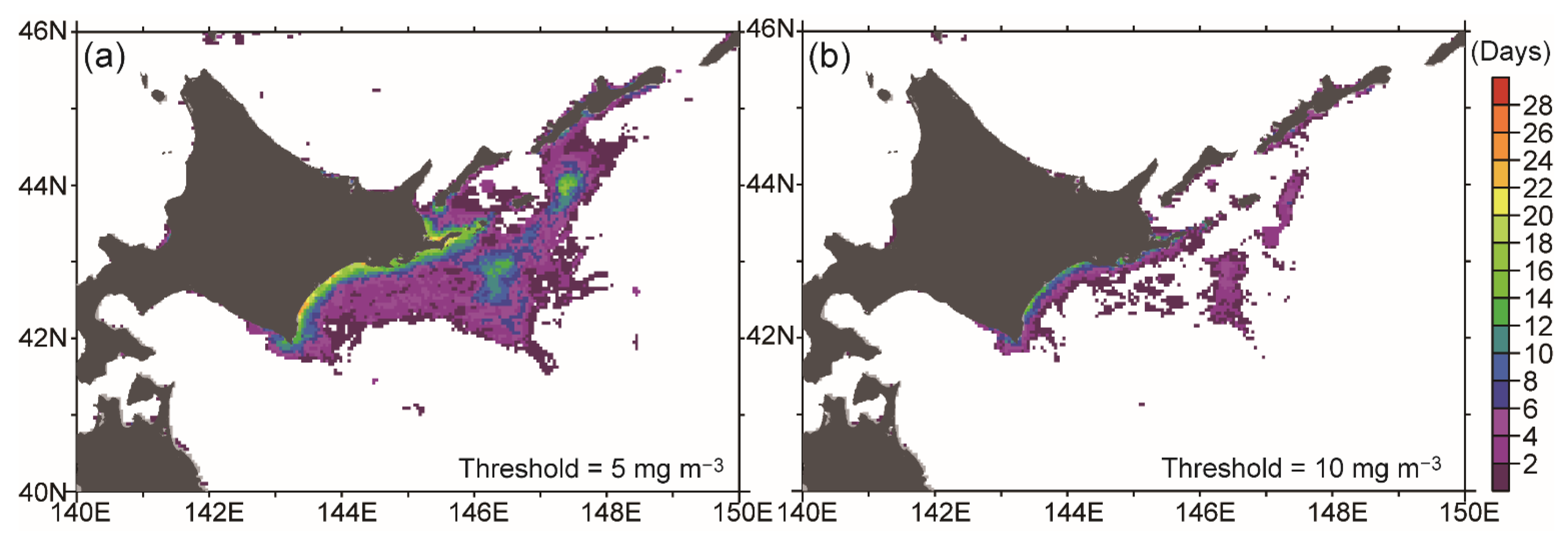
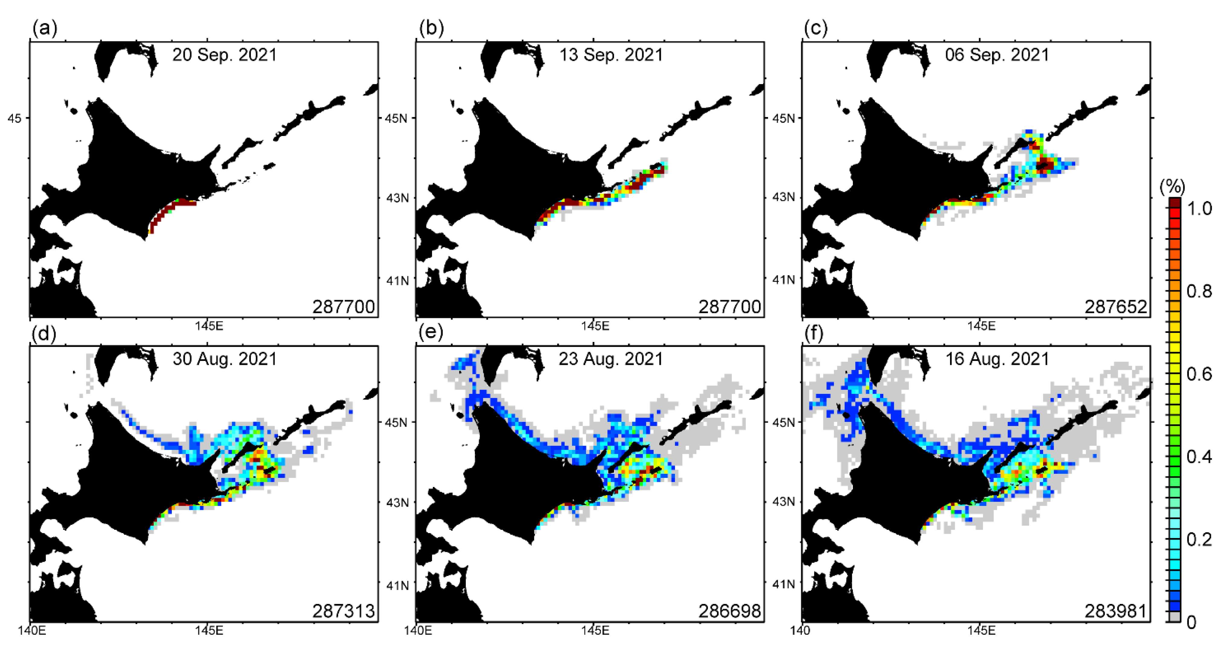
3.1. Satellite-Derived Chlorophyll Concentration

Figure 3 shows maps of daily SCCs, which were associated with the process of HAB development. In these maps, SCCs exceeding the mean plus three standard deviations at individual grid cells (i.e., extremely high SCCs) are emphasized by black polygons. At the end of August (Figure 3a), relatively high SCCs started to appear around the study region but hardly exceeded 10 mg m−3. At the beginning of September (Figure 3b), SCCs increased abruptly south of Etorofu Island and exceeded 10 mg m−3 near the centre of patch-like local maxima. On 7 September (Figure 3c), the area of the patch-like SCCs increased, and the patches seemed to expand south-westward to the south of Shikotan Island. On 14 September (Figure 3d), the patch-like local maximum became less distinct, and the patch elongated in a clockwise direction on the continental slope, probably because of the combined effects of horizontal advection and diffusion. At the same time, high SCCs (>5 mg m−3) suddenly appeared along the entirety of the Pacific coast off southeast Hokkaido. On 20 September (Figure 3e), the SCCs increased dramatically and exceeded 10 mg m−3 in coastal shelf waters along the Hokkaido coast and in slope waters. On 27 September (Figure 3f), the area of high SCCs (>10 mg m−3) in coastal shelf waters expanded slightly in an offshore direction, and the high SCCs in slope waters decreased and were mostly lower than 10 mg m−3. These results implied that occurrence of HABs was localized around the Four Islands and along the southeast coast of Hokkaido. The HABs were, therefore, isolated from the surrounding waters off the Kuril Islands and in the Sea of Okhotsk.
To examine the areal extent of high SCCs in 2021(Figure 4), we integrated the area of a grid cell with SCCs exceeding 5 or 10 mg m−3 over the pink rectangular region (hereafter “focal region”) in Figure 3 In situ chlorophyll a concentrations > 5 mg m−3 have been used as typical indicators of massive spring blooms in the Oyashio area [48]. The area of high SCCs started to increase slowly after the middle of August 2021. After late August, the area intermittently became comparable to the climatological daily maximum over 23 years (1998–2020), i.e., the upper boundary of red shading in Figure 4. The area then increased dramatically in mid- to late September 2021. At that time, the area was sometimes more than twice as large as the 23-year daily maximum area. The 23-year daily maximum area was also comparable to the mean plus 3 standard deviations (blue line in Figure 4). The implication was that the area of high SCCs in mid-to-late September sometimes reached the mean plus six standard deviations. The large area of the high SCCs in mid-to-late September 2021 could, therefore, be interpreted as a very rare, extreme phenomenon.
Next, to examine the duration of the high SCCs in 2021, we counted the number of days during September 2021 when the SCCs exceeded 5 or 10 mg m−3 at each grid (Figure 5). Long durations were apparent around the Pacific coastal, shelf, and slope regions off the Four Islands and southeast of Hokkaido. The duration tended to be longer near the coast and shorter offshore, except for the elongated local maximum that extended south-westward from Etorofu Island. In coastal waters off southeast Hokkaido, the durations exceeded 20 (10) days for the threshold of 5 (10) mg m−3. For the region illustrated in Figure 5, 74% of the areas that exceeded the threshold SCC of 5 mg m−3 and 76% of the areas that exceeded the threshold SCC of 10 mg m−3 exhibited the longest duration of exceedance of the respective thresholds during September in 1998–2021. The implication was that the persistence of the high SCCs measured around the focal region broke historical records in September 2021.

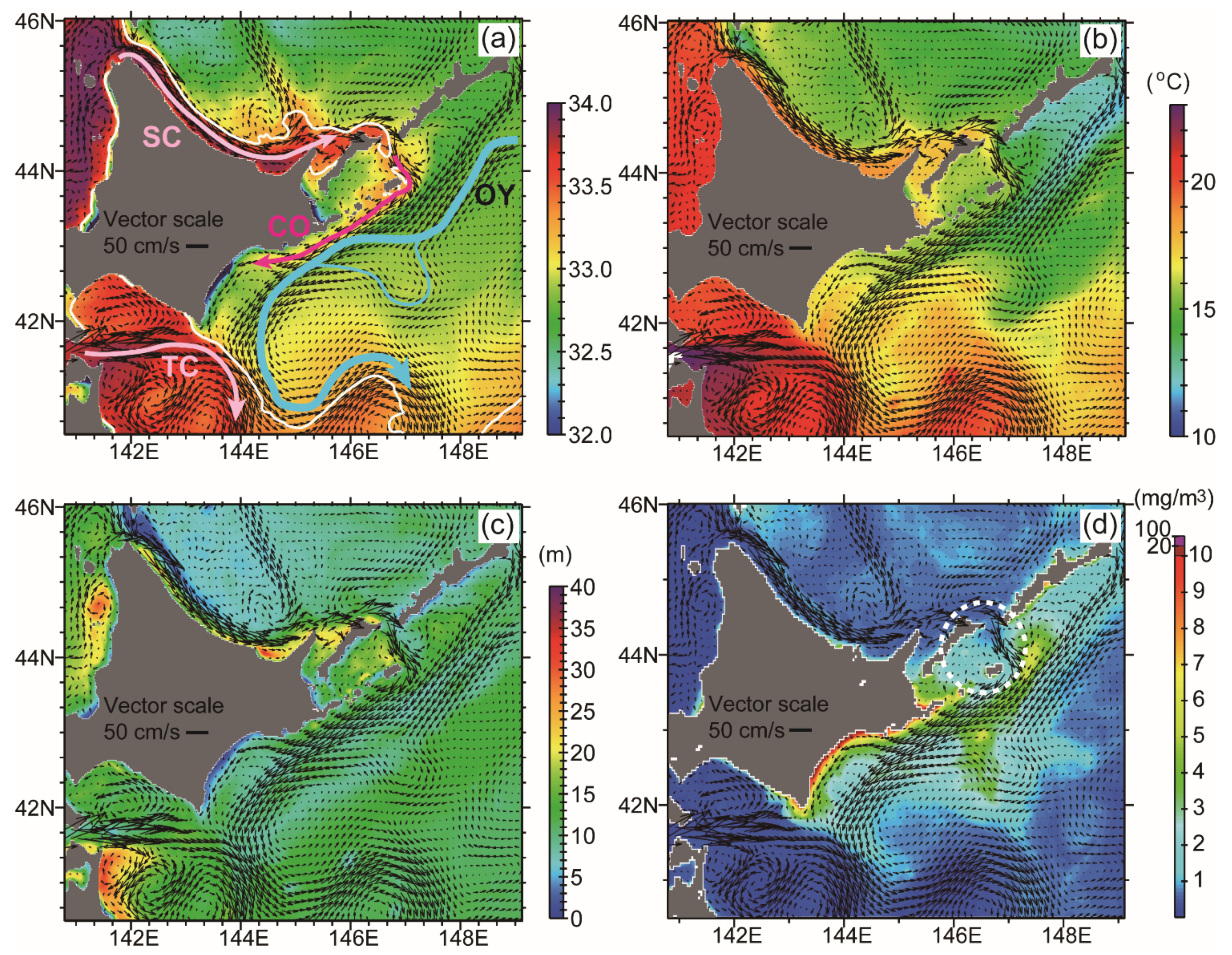
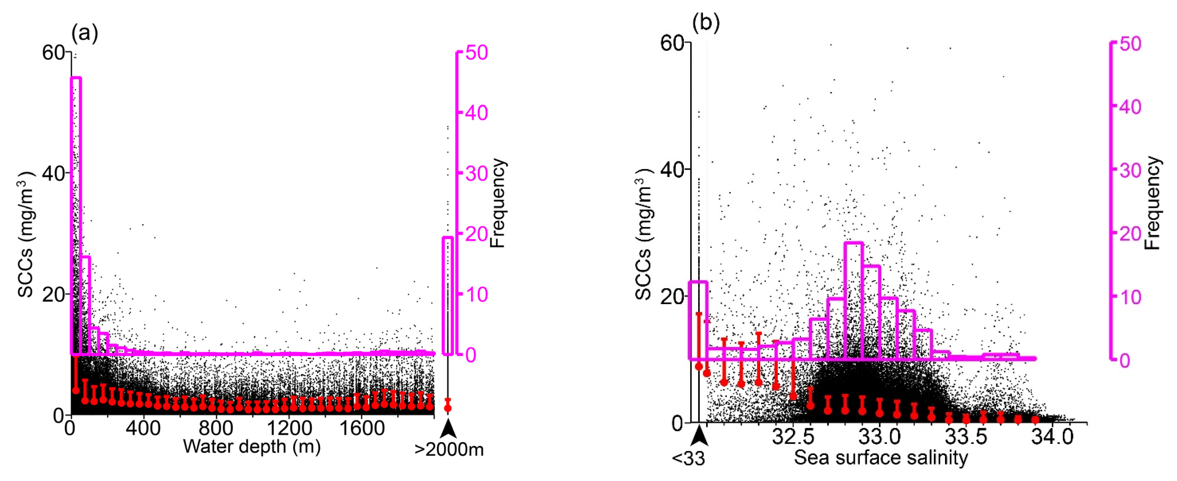
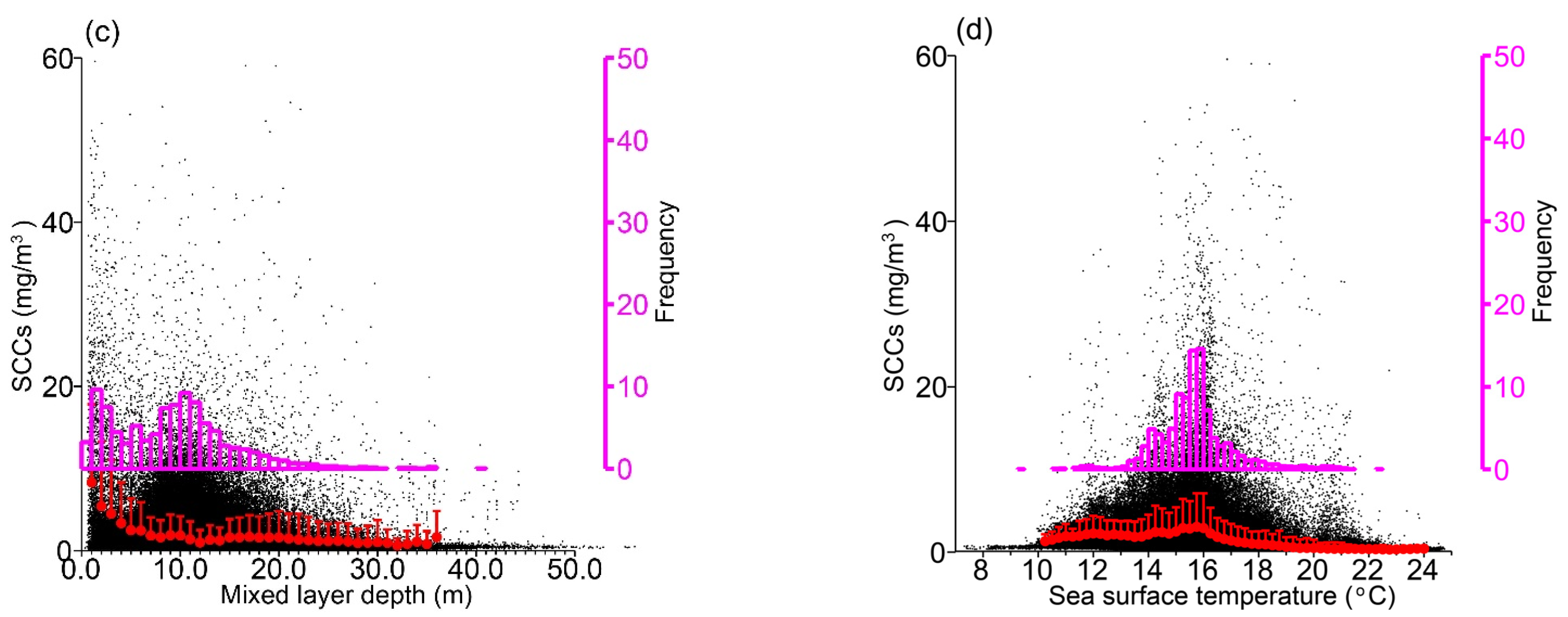
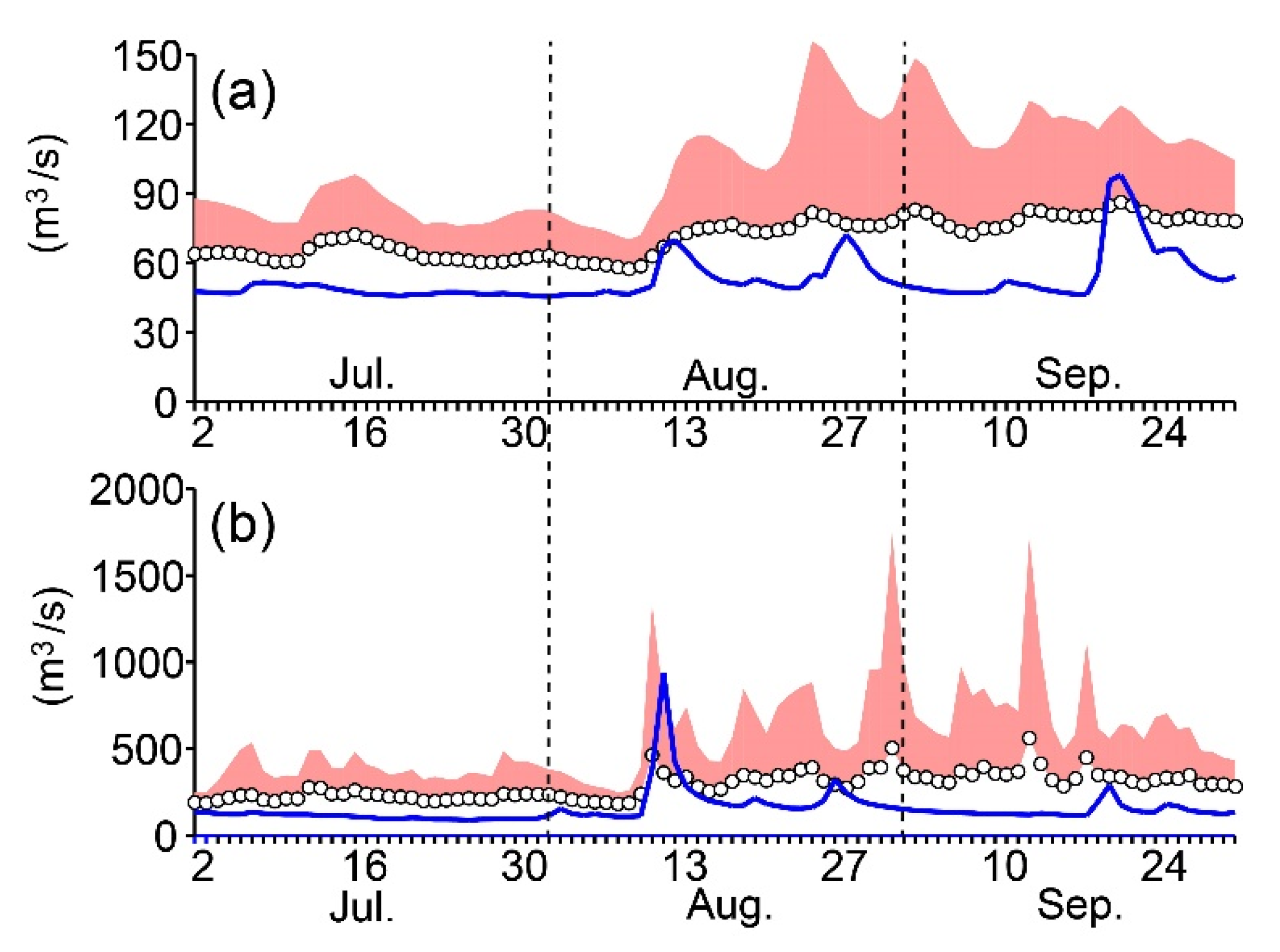
3.2. Relationships to Environmental Conditions

To understand relationships between high SCCs (i.e., potential occurrence of HABs) and oceanographic conditions, we analyzed outputs from the 1/50° ocean model. Monthly mean salinities and current velocities at the sea surface (Figure 6a) reflected representative ocean current conditions around Hokkaido in September 2021. The Oyashio flowed from the northeast to the southwest along the continental slope. A part of the Oyashio bifurcated to the south of Shikotan Island, was deflected in a clockwise direction, and then rejoined the mainstream of the Oyashio. Meanwhile, the Soya Warm Current, which is characterized by high-salinity water (>33.5), flowed along the Okhotsk coast of northeast Hokkaido and intruded into the Kunashiri Strait. Water with relatively high salinity (~33.5) that outflowed into the Pacific shelf was then transported in a south-westward direction by the Coastal Oyashio onto the Pacific shelf, inshore of the Oyashio on the slope. The salinity along the Coastal Oyashio decreased gradually downstream from the Kunashiri Strait. The implication was that Soya Warm Current water was modified by mixing with the surrounding low-salinity waters, and so-called modified Soya Warm Current water was formed on the Pacific shelf. On the inshore side of the Coastal Oyashio, water with very low salinity (<32.5) due to river discharge was distributed along the Hokkaido coast. A sharp water-mass front along the 33.3 isohaline (white contour line in Figure 6a) was apparent around Cape Erimo between subtropical waters supplied from the Tsugaru Strait and subarctic waters around the Oyashio. The front meandered along the southern edge of the Oyashio.
We compared a map of monthly mean SCCs (Figure 6d) with the simulated salinities. Overall, relatively high SCCs tended to be distributed within the inshore side of the Oyashio mainstream (i.e., coastal shelf waters), except in the vicinity of the clockwise bifurcation of the Oyashio on the slope, south of the Shikotan Island. Particularly high SCCs (~10 mg m−3) were distributed in very nearshore waters along the southeast Hokkaido coast, where river discharges resulted in very low-salinity waters. The surface mixed layers were also very shallow in those waters (~a few meters) (Figure 6c). It is noteworthy that SCCs along the mainstream of the Soya Warm Current were quite low (<1 mg m−3). In addition, around the southern entrance of the Kunashiri Strait and Shikotan Island (see thick dashed ellipse in Figure 6d), where Soya Warm Current water was supplied from the Sea of Okhotsk throughout summer and autumn, SCCs were also lower (<3 mg m−3) than in the surrounding Pacific shelf waters. Moreover, there was an abrupt transition from low to high SCCs between the western and eastern side, respectively, of the sharp salinity front south of Cape Erimo. These results suggested that the high SCCs associated with HABs were less intense in subtropical, high-salinity waters.
To obtain a more quantitative understanding of the relationships between SCCs and environmental variables, we created four scatter plots of SCCs versus water depths, sea surface salinities, sea surface temperatures, and surface mixed layer depths. In Figure 7, we have plotted daily SCCs based on the L3 product in only Pacific waters versus the daily means of variables. Bin-averaged SCCs (filled red circles) and the frequency distributions for SCCs exceeding 10 mg m−3 (pink bar chart) overlay the scatter diagrams. Scatter plots based on monthly means (e.g., Figure 6) exhibited similar features, but there were fewer data points (not shown).
Water depth was a primary determinant of the occurrence of SCCs that exceeded 10 mg m−3 (Figure 7a); both bin-averaged means and frequencies of high SCCs increased toward shallow water depths. 72% of the SCCs that exceeded 10 mg m−3 occurred in water depths of 0–300 m, which corresponded to locations near the coast, shelf, and shelf break. 9% and 19% of the high SCCs were associated with water depths of 300–2000 and >2000 m, respectively. Sea surface salinity and mixed layer depth exhibited similar relationships with SCCs; their frequency distributions exhibited two local maxima. The two maxima could be interpreted to reflect the different conditions associated with high SCCs in nearshore and shelf waters. As mentioned before, the nearshore waters were characterized by very low salinities and very shallow mixed layer depths (Figure 6a,c). Those conditions corresponded to the peaks on the sides of Figure 7b,c. The high SCCs in the shelf waters corresponded to the peaks on the right sides of the same figures at a salinity of 32.8 (Figure 7b) and mixed layer depth of 10 m (Figure 7c). In addition, high SCCs appeared less frequently in water with a high salinity (>33.3) and at locations where the mixed layer exceeded 20 m. These conditions were associated with subtropical waters (Figure 6a,c). However, part of the modified Soya Warm Current water, typically with a salinity of 33.0–33.7, contributed to the peak at high salinity ~32.8 and a mixed layer depth ~10 m. The frequency distribution of high SCCs as a function of sea surface temperature (Figure 7d) exhibited a single peak at around 16°C and differed distinctly from the bimodal salinity and mixed layer depth distributions. Sea-surface temperatures could therefore not be used to distinguish between the high SCCs in nearshore and shelf waters.
It is here emphasized that sea surface salinities simulated by the 1/50° ocean model had low-salinity bias of about 0.2 in autumn around the focal region (e.g., [25]), which was reconfirmed by comparison with in situ sea surface salinities along the A-line (e.g., [22]) that were measured on 4–10 October 2021 (not shown).
To identify the factors possibly responsible for the anomalous increase in the daily areal extent of high SCCs after late August (i.e., Figure 4), we estimated the mixed layer depths at grid cells with SCCs of >5 or >10 mg m−3, and averaged those mixed layer depths for each day (Figure 8a–d). We refer to those averages as “high-chlorophyll mixed layer depths”. The mixed layer depth is here regarded as a metric of nutrient supply from the subsurface to the vicinity of the sea surface via vertical convection/entrainment. The high-chlorophyll mixed layer depths were roughly correlated with the extent of high SCCs (Figure 8b,d). High-chlorophyll mixed layer depths of approximately 10 m corresponded to the largest area, which appeared in mid-to-late September (Figure 8a,c). A mixed layer depth of 10 m was also related to the right peak of the frequency distribution of high SCCs as a function of mixed layer depth (Figure 7c).
The high-chlorophyll mixed layer depths continued to be very shallow until the beginning of August (Figure 8a,c), when the marine heatwaves reached a maximum (Figure 8e), and they deepened abruptly on 10 August, when the marine heatwaves retreated abruptly. After mid-August, when the marine heatwaves ended, the high-chlorophyll mixed layer depths tended to increase gradually to the end of September. Simulated vertical eddy diffusivity near the sea surface averaged over the focal region also continued to increase after the spike-like increase on 10 August (Figure 8e). It is noteworthy that the area of high SCCs increased slowly after mid-August, started to intermittently exceed the climatological daily maximum after late August, and reached a record-breaking extent in mid-to-late September (Figure 4). As a result, the extreme expansion of the area of high SCCs associated with the occurrence of massive HABs was tightly linked with deepening of mixed layer depths in subarctic waters beginning at the time of the abrupt end of the marine heatwaves.
However, the deepening of the mixed layer depths could not explain the abrupt increase in SCCs (i.e., intensification of HABs) in very nearshore waters along the southeast Hokkaido coast (Figure 3d–f), where a very shallow mixed layer depth was related to river-influenced, very-low-salinity water that contained high SCCs (e.g., Figure 7b,c). River discharge into coastal waters were examined as a potential controlling factor (e.g., [15]), but there was little evidence of abnormal discharge conditions during the summer of 2021 (see Appendix A). As a result, the mechanism responsible for the abrupt growth of the harmful algae and a mechanism responsible for their accumulation (e.g., biological aggregation or physical convergence) needed to be identified.

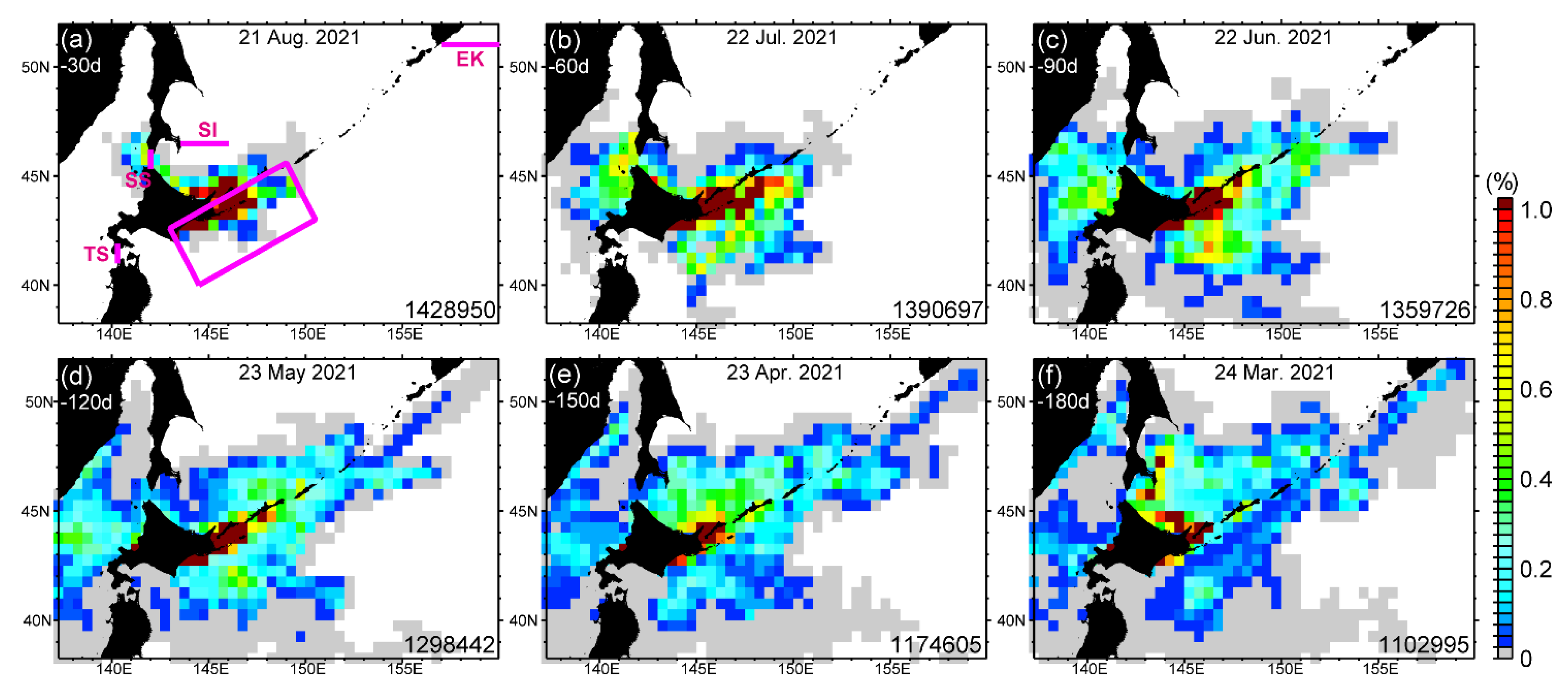
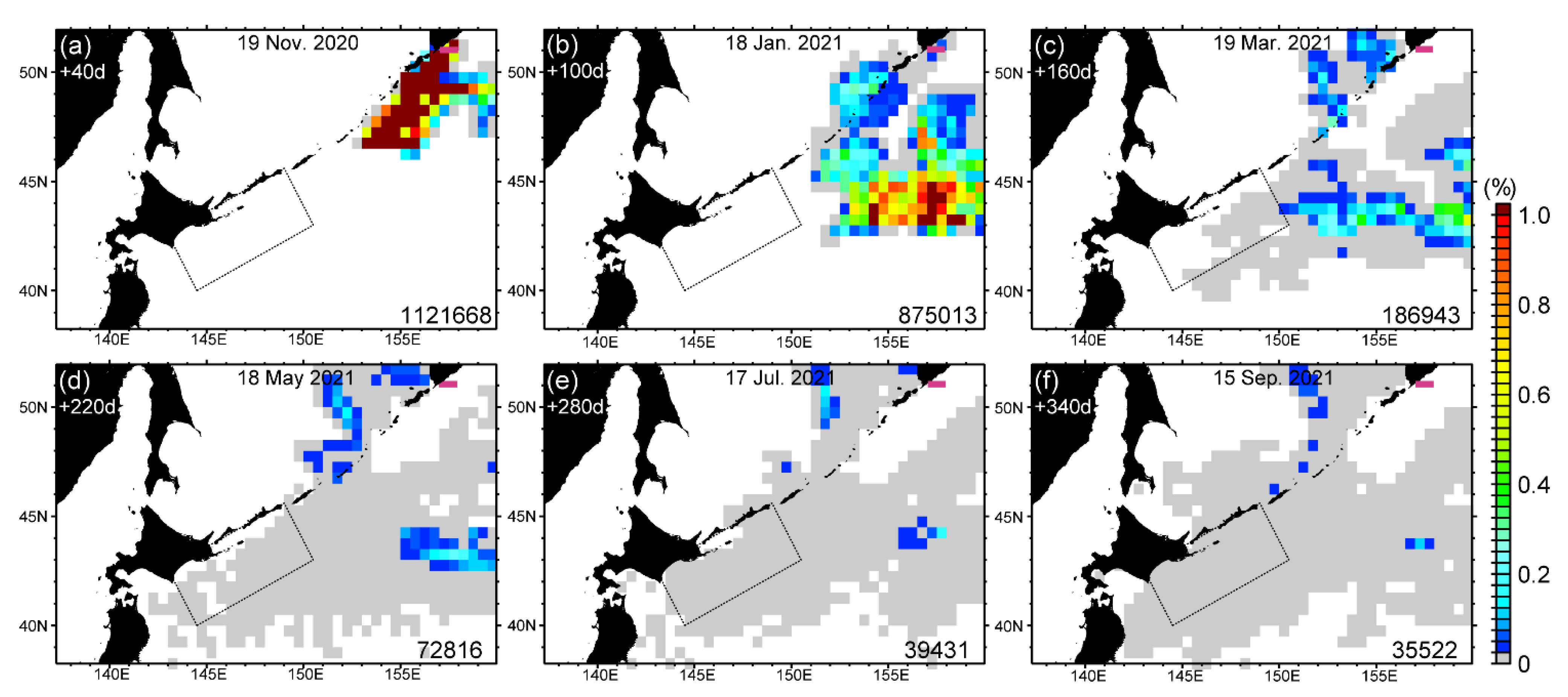
3.3. Potential Sources of HABs

To identify the area that was likely the source of the HABs, we first performed retrospective particle-tracking simulations (Figure 9). Some of the particles were transported from their positions in the blooms backward in time along the main stream of the Coastal Oyashio and Soya Warm Current. More specifically, particles were tracked from their positions in the blooms in an eastward direction along the Pacific shelf (Figure 9a,b), and then from the Pacific shelf through the Kunashiri Strait to the shelf along the north-eastern coast of Hokkaido in the Okhotsk Sea (Figure 9c,d). The particles then passed through the Soya Strait (Figure 9e) and finally reached the Sea of Japan (Figure 9f). The minimum elapsed time was 21–28 days, at least for particles to be transported retrospectively from their positions in the blooms to the Sea of Japan. Hence, one of the potential source areas was the Sea of Japan. Shimada et al. [49] have identified the presence of the dinoflagellate K. mikimotoi near the Hokkaido coast in the Tsugaru Strait during autumn of 2015 for the first time and suggested that there was horizontal transport of the harmful algae from the Sea of Japan. Our results were consistent with the potential source area that they suggested.
Next, we examined whether harmful algae could have been passively transported by ocean currents to the focal region from the Pacific Ocean east of the Kamchatka Peninsula, where a massive bloom of the dinoflagellate K. selliformis occurred during September–October 2020 [18], with a focus on wider area and longer tracking time (Figure 10). Particles that were transported retrospectively to the northeast along the Oyashio and the East Kamchatka Current travelled the longest distance. It took about 4 months, at least, for the particles to be transported retrospectively from coastal waters off southeast Hokkaido to the area east of the Kamchatka Peninsula (Figure 10d–f).
Moreover, note that a large number of particles were transported back to the southern part of the Sea of Okhotsk (Figure 10). In March 2021, particles were densely distributed along the east coast of the southern part of the Sakhalin Island (Figure 10f), which indicated that particles were prospectively transported southward by the East Sakhalin Current intensified in winter. Orlova et al. [50] also reported that K. mikimotoi was identified during June–October in 1994 and 1998–2000 near the east coast of the Sakhalin coast between 46°30′ N and 53° N. Therefore, the vicinity of this area could be also regarded as potential source areas.
The numbers of particles passing through the following four transects were counted at daily intervals (Figure 11a): (1) a meridional transect in the Tsugaru Strait, (2) a meridional transect in the Soya Strait, (3) a zonal transect from 143°30′ E to 146° E east of the Sakhalin Island, and (4) a zonal transect east of the Kamchatka Peninsula (see Figure 10a). For particles passing through the transect in the Soya Strait, the number of particles started to increase after the 20-day tracking period, reached a maximum during the 30–60-day tracking period (i.e., July–August), and then decreased abruptly. Meanwhile, the number of particles passing through the transect in the Tsugaru Strait was nearly zero throughout the particle-tracking period. The number of particles passing through the transect east of the Sakhalin Island increased remarkably from 135-day tracking period (i.e., mid-April). This result indicated that particles prospectively left the east coast of the Sakhalin Island in winter, when particles were actively transported southward together with sea ice–related very cold waters with a nearly freezing temperature by the East Sakhalin Current. Moreover, the number of particles passing through the transect east of the Kamchatka Peninsula was zero until roughly the 100-day tracking period (i.e., mid-May). It then increased and fluctuated. Hence, if the ocean east of the Kamchatka Peninsula had been the source of the HABs off southeast Hokkaido, a transport period of more than four months would have been needed.
To investigate linkages between HABs that developed east of the Kamchatka Peninsula in late summer 2020 to those that developed in the focal region in late summer 2021, we analyzed results from particle-tracking simulations forward in time that released a large number of particles from the vicinity of the Pacific Ocean east of the Kamchatka Peninsula during 30 September to 20 October 2020 (Figure 12). Most particles started to be transported to the southwest at the beginning of the particle-tracking period (Figure 12a). A large percentage of the particles were then greatly dispersed horizontally and transported outside of the particle-tracking domain through the eastern boundary until the tracking time reached 160 days (approximately mid-March 2021) (Figure 12b,c). The rest of the particles were partially transported south-westward along the East Kamchatka Current and the Oyashio, and some of them reached the focal region of the study (Figure 12d–f). In July–September 2021, only a small percentage of the particles (~0.3% relative to the number of initially released particles) remained in the focal region (Figure 13). These results, therefore, implied that growth of harmful algae during the period of passive transport would have been essential if HABs in the Pacific Ocean to the east of the Kamchatka Peninsula in the late summer of 2020 were the cause of the blooms in the focal region in the late summer of 2021, but that possibility was not included in our particle-tracking simulation.

4. Discussion

4.1. Possible Linkages from Algal Transport to Outbreak

Particle-tracking simulations identified three potential source areas: the Pacific Ocean east of the Kamchatka Peninsula, the Sea of Japan, and the Sea of Okhotsk east of the Sakhalin Island. It is noteworthy that the high SCCs apparent around the focal region in late summer 2021 were isolated from the surrounding waters of the Pacific Ocean and Sea of Okhotsk (e.g., Figure 3). High SCCs were also not observed along the transport pathways from the potential sources to the focal region. These facts allowed us to hypothesize that harmful algae or their seeds were transported from the potential source areas to the focal region without generating blooms, and the algae finally generated massive blooms within the focal region when they encountered optimal environmental conditions.
This hypothesis is probably reasonable for the algae transported from the Sea of Japan, because our results indicated that high SCCs were less frequently observed in subtropical, high-salinity waters (e.g., Figure 7b). Along the transport pathway from the Sea of Japan to the focal region, harmful algae or seeds could be transported together with oligotrophic subtropical waters by the Tsushima Warm Current and Soya Warm Current.
The cases for the Sea of Okhotsk east of the Sakhalin Island and the Pacific Ocean east of the Kamchatka Peninsula are more complex, principally because the transport time of the algae would have been longer (>4 months), and the algae would have been transported together with subarctic waters by the East Sakhalin Current, East Kamchatka Current, and Oyashio. The long transport time forced us to consider biological growth of the harmful algae, as mentioned in Section 3.3. If these two pathways were feasible, the subarctic waters along the transport pathways might have suppressed the growth of the algae. In general, subarctic waters exhibit nutrient-rich conditions, associated with enhancement of algal growth. Therefore, light-deficient associated with a persistently deep mixed layer induced by strong tidal mixing [51,52], and/or reduction in growth attributed to very cold temperatures could have inhibited outbreaks of harmful algae during the transport period.
We want to stress that ocean circulation near the sea surface in the focal region is characterized by high retention of particles. As shown in Figure 11b, a large number of particles remained within the focal region, even after a long period of particle tracking. More specifically, about 60%, 40%, and 20% of the particles initially released remained within the focal region after retrospective tracking periods of 60, 120, and 180 days, respectively. In addition, the number of particles distributed within the focal region during the prospective particle-tracking simulation became nearly constant after June of 2021 (Figure 12). The implication is that the focal region very efficiently retained particles. In other words, once particles were transported into the focal region, it was difficult for them to exit. The high particle retention by the focal region might have allowed the harmful algae to remain in the focal region until environmental conditions became favourable for massive blooms.
HABs that included both K. mikimotoi and K. selliformis have been identified off the Hokkaido coast. According to Shimada et al. [49], a potential source of the K. mikimotoi distributed around Hokkaido is the Sea of Japan. Orlova et al. [50] also identified K. mikimotoi near the east coast of the Sakhalin Island. These results are consistent with two potential source areas identified by our particle-tracking simulations. Moreover, our particle-tracking simulations revealed that the Pacific Ocean to the east of the Kamchatka Peninsula could be the other potential source. This possibility is consistent with the outbreaks of K. selliformis in September–October 2020 [18,19]. These observations lead to the hypothesis that different algal species may have been separately transported from the three potential source areas and contributed simultaneously to the occurrence of the HABs off the southeast coast of Hokkaido in late summer of 2021.

4.2. Relationship of Algal Outbreaks to Marine Heatwaves

It is very instructive to remember that the massive HABs in the Pacific Ocean near the east coast of the Kamchatka Peninsula in the late summer of 2020 followed extreme marine heatwaves that occurred in both June and July of 2020, when the maximum anomalies of sea surface temperature reached about 6 °C [18]. The magnitude and timing of the second marine heatwave and the time lag between the second marine heatwave and the HABs were very consistent with the sequence of events in this study. In the case of the Pacific Ocean to the east of the Kamchatka Peninsula, a large influx of nutrients came from river discharge. In our focal region, entrainment of subsurface waters by deepening of the mixed layer over the shelf was an important source of nutrients. The 10 m depth of the mixed layer in the low-salinity, subarctic waters likely provided optimal conditions for blooming of harmful algae during September 2021 (Figure 7b,c), i.e., there was a sufficient supply of both nutrients and light. The importance of uplifted nutrients to the occurrence of HABs has likewise been stressed by McCabe et al. [53], who attributed large HABs along the North American west coast associated with marine heatwaves to seasonal coastal upwelling.
Numerous studies have also reported that marine heatwaves have triggered massive HABs in many places globally [18,53,54,55,56,57,58,59,60,61]. However, the process and mechanism, namely, how marine heatwaves trigger HABs, has not been accurately understood. Additional studies for clarification are thus essential to mitigate the impacts of HABs on human life. It is difficult, however, to repeatedly monitor HABs triggered by marine heatwaves in a specific ecosystem, because marine heatwaves are climate extremes (i.e., rare events) in the ocean systems. Interregional studies are the best way to compare HABs triggered by marine heatwaves among different marine ecosystems and to understand the relevant mechanisms and predict the occurrence of HABs.

5. Conclusions

How can we most efficiently develop an understanding of the impact of extreme events on marine ecosystems and relate those impacts to environmental conditions? One of the most robust methodologies is analysis by combining near-real-time ocean monitoring with realistic ocean modelling. Unprecedented outbreaks of harmful algae were reported in the late summer of 2021 in coastal waters off southeast Hokkaido, one month after the most intense and extensive marine heatwaves in the north-western Pacific Ocean had subsided. Just after the marine heatwaves subsided (~20 August), the areal extent of the high SCCs began to slowly increase. The area of high SCCs occasionally exceeded the climatological maxima after late August and finally reached the most extreme record-breaking level (~mean plus 6 standard deviations) in mid-to-late September. The expansion of the area was accompanied by a deepening of surface mixed layer depths that began after the terminal phase of the marine heat waves. That deepening of the mixed layer was associated with an influx of nutrients from the subsurface via vertical convection/entrainment.
About 70% of the high SCCs that exceeded 10 mg m−3 were observed in coastal shelf waters with water depths < 300 m. Characteristics of the high SCCs clearly differed between nearshore waters and shelf waters. The nearshore waters were strongly influenced by river discharge, i.e., the salinity was very low, and the mixed layer was very shallow (~a few meters). The waters over the shelf with high SCCs corresponded to subarctic waters with mixed layer depths of about 10 m. In other words, the high SCCs rarely occurred in subtropical waters.
Retrospective particle-tracking simulations revealed three potential source areas of the HABs that occurred in the coastal waters of the Pacific Ocean off southeast Hokkaido: the Pacific Ocean to the east of the Kamchatka Peninsula, the Sea of Japan, and the Sea of Okhotsk east of the Sakhalin Island. The transport time from the potential source areas differed greatly: about 1–2 months for the second potential source area and >4 months for the others. Prospective particle-tracking simulations also indicated that when particles were released from coastal waters off the east coast of the Kamchatka Peninsula in October 2020 on the assumption that a massive HAB had occurred there, ~0.3% of the particles initially released reached the focal region in July–September of 2021 and stagnated there because the focal area seems to very efficiently retain particles. The very small percentage of ~0.3% implied that algal growth during the period of passive transport over the long distance would have been essential to cause the subsequent massive HABs, although that possibility was completely neglected in our simulations. In any case, it is needed for future work to verify the validity of each potential source area by examining in situ distribution of Karenia species in 2020–2021 around the three potential transport pathways.
Finally, we want to note two weaknesses of this study. The first weakness was that the study focused merely on the development stage of the HABs. The HABs seemed to be declining as of 15 November 2021. The processes associated with this decline need to be examined in subsequent work. The second weakness of this study was that it included some biases. According to Kuroda et al. [25], for instance, sea surface salinity estimated with a 1/50° ocean model in coastal shelf waters off the southeast coast of Hokkaido in autumn 2016 exhibited a low-salinity bias by about 0.2. This bias suggested that the biological-physical relationships revealed by this study should be based on relative values of environmental conditions (e.g., Figure 7). These model biases need to be corrected by comparisons with in situ measurements in future work to precisely understand biological phenomena in relation to absolute values of environmental variables. In addition, the SCCs are associated with interpretative biases. Specifically, high SCCs might not be entirely attributable to the occurrence of HABs. It is possible that non-harmful algae might increase in abundance, particularly in offshore waters. Our study should, therefore, be confirmed and could be improved by accumulating scientific data based on in situ measurements. Nevertheless, we emphasize that analyses combining satellite monitoring and realistic ocean modelling are very useful for immediately overviewing the entirety of a phenomenon, even if it is an unprecedented, extreme event.

Author Contributions

Conceptualization, H.K., T.A. and N.H.; methodology, H.K.; software, T.S.; validation, T.A.; writing—original draft preparation, H.K.; writing—review and editing, T.A. and T.S.; visualization, H.K.; project administration, N.H.; funding acquisition, H.K. All authors have read and agreed to the published version of the manuscript.

Funding

This research was supported by the Environment Research and Technology Development Fund (4-2102) of the Environmental Restoration and Conservation Agency of Japan. This work was also partly supported by the Fisheries Agency (no grant number), but the contents of this study do not necessarily reflect the views of the Fisheries Agency.

Institutional Review Board Statement

Not applicable.

Informed Consent Statement

Not applicable.

Data Availability Statement

Gridded data of chlorophyll concentrations from ocean color sensors were downloaded from a webserver of the European Union’s Copernicus Marine Service (accessed on 12 October 2021). Daily reanalysis data from FRA-ROMS are available at http://fm.dc.affrc.go.jp/fra-roms after user registration (accessed on 12 October 2021). The source code of the 1/50° model based on Rutgers University’s ROMS is available at https://www.myroms.org (accessed on 17 February 2010). All external forcings for the 1/50° model (NAO.99Jb, GPV/MSM, JRA55, and river discharge data) are also publicly available. The original LTRANS code was downloaded from https://northweb.hpl.umces.edu/LTRANS.htm (accessed on 4 September 2012).

Acknowledgments

Numerical experiments based on FRA-ROMS were conducted using the Scientific Computing System in the Agriculture, Forestry and Fisheries Research Information Technology Center. We extend a special thanks to associate editors, and three reviewers for many constructive and fruitful comments.

Conflicts of Interest

The authors declare no conflict of interest.

Appendix A

This appendix briefly describes conditions of river discharge in July–September 2021. There are two primary water systems (i.e., the Kushiro and Tokachi rivers) in southeast Hokkaido (Figure 1b). Figure A1 shows time series of daily mean discharge, which was given to the 1/50° model, in comparison to the climatological daily mean and the standard deviations during 1992–2020. Daily mean discharges in 2021 were estimated from near-real-time river surface height by using a previously determined quadratic regression curve between river discharge and river surface height. The daily mean discharge from the two rivers was lower than the climatological mean throughout most of the summer of 2021. Discharge intermittently increased three times (i.e., 10 August, 26 August, and 20 September), but the individual maxima were comparable to the climatological mean, except for the discharge from the Tokachi River on 10 August (~mean plus one standard deviation).
Figure A1. Daily discharge from the (a) Kushiro River and (b) Tokachi River (thick blue line) in 2021. Climatological daily means (1992–2020) and means plus one standard deviation are denoted by open circles and red shading, respectively.
Jmse 09 01335 g0a1

References

  1. Morris, J.G., Jr. Harmful algal blooms: An emerging public health problem with possible links to human stress on the environment. Annu. Rev. Environ. Resour. 1999, 24, 367–390. [Google Scholar] [CrossRef]
  2. Anderson, D.M.; Hoagland, P.; Kaoru, Y.; White, A.W. Estimated annual economic impacts from harmful algal blooms (HABs) in the United States. WHOI Tech. Rep. 2000, 2000–2011. [Google Scholar] [CrossRef] [Green Version]
  3. Anderson, D.M.; Cembella, A.D.; Hallegraeff, G.M. Progress in understanding harmful algal blooms (HABs): Paradigm shifts and new technologies for research, monitoring and management. Ann. Rev. Mar. Sci. 2012, 4, 143–176. [Google Scholar] [CrossRef] [Green Version]
  4. Berdalet, E.; Fleming, L.E.; Gowen, R.; Davidson, K.; Hess, P.; Backer, L.C.; Moore, S.K.; Hoagland, P.; Enevoldsen, E. Marine harmful algal blooms, human health and wellbeing: Challenges and opportunities in the 21st century. J. Mar. Biol. Assoc. UK 2015, 96, 61–91. [Google Scholar] [CrossRef] [Green Version]
  5. Brown, A.R.; Lilley, M.; Shutler, J.; Lowe, C.; Artioli, Y.; Torres, R.; Berdalet, E.; Tyler, C.R. Assessing risks and mitigating impacts of harmful algal blooms on mariculture and marine fisheries. Rev. Aquac. 2020, 12, 1663–1688. [Google Scholar] [CrossRef] [Green Version]
  6. Sakamoto, S.; Lim, W.A.; Lu, D.; Daic, X.; Orlova, T.; Iwataki, M. Harmful algal blooms and associated fisheries damage in East Asia: Current status and trends in China, Japan, Korea and Russia. Harmful Algae 2021, 102, 101787. [Google Scholar] [CrossRef]
  7. Imai, I.; Yamaguchi, M.; Hori, Y. Eutrophication and occurrences of harmful algal blooms in the Seto Inland Sea, Japan. Plankton Benthos Res. 2006, 1, 71–84. [Google Scholar] [CrossRef] [Green Version]
  8. Trainer, V.L.; Moore, S.K.; Hallegraeff, G.; Kudela, R.M.; Clement, A.; Mardones, J.I.; Cochlan, W.P. Pelagic harmful algal blooms and climate change: Lessons from nature’s experiments with extremes. Harmful Algae 2020, 91, 101591. [Google Scholar] [CrossRef]
  9. León-Muñoz, J.; Urbina, M.A.; Garreaud, R.; Iriarte, J.L. Hydroclimatic conditions trigger record harmful algal bloom in western Patagonia (summer 2016). Sci. Rep. 2018, 8, 1330. [Google Scholar] [CrossRef] [Green Version]
  10. Moore, K.M.; Allison, E.H.; Dreyer, S.J.; Ekstrom, J.A.; Jardine, S.L.; Klinger, T.; Moore, S.K.; Norman, K.C. Identifying effective adaptive actions used in fishery-dependent communities in response to a protracted event. Front. Mar. Sci. 2020, 6, 803. [Google Scholar] [CrossRef]
  11. Phips, E.J.; Badlak, S.B.; Nelson, N.G.; Havens, K.E. Hurricanes, El Niño and harmful algal blooms in two sub-tropical Florida estuaries: Direct and indirect impacts. Sci. Rep. 2020, 10, 1910. [Google Scholar] [CrossRef] [PubMed] [Green Version]
  12. Bondur, V.G.; Zamshin, V.V.; Chvertkova, O.I. Space study of a red tide-related environmental disaster near Kamchatka Peninsula in September–October 2020. Dokl. Earth Sci. 2021, 497, 255–260. [Google Scholar] [CrossRef]
  13. Lim, Y.K.; Park, B.S.; Kim, J.H.; Baek, S.S.; Baek, S.H. Effect of marine heatwaves on bloom formation of the harmful dinoflagellate Cochlodinium polykrikoides: Two sides of the same coin? Harmful Algae 2021, 104, 102029. [Google Scholar] [CrossRef]
  14. Kuroda, H.; Setou, T. Extensive marine heatwaves at the sea surface in the northwestern Pacific Ocean in summer 2021. Remote Sens. 2021, 13, 3989. [Google Scholar] [CrossRef]
  15. Shimada, H. Long-term fluctuation of red tide and shellfish toxin along the coast of Hokkaido (Review). Sci. Rep. Hokkaido Fish. Res. Inst. 2021, 100, 1–12, (In Japanese with English abstract). [Google Scholar]
  16. Haywood, A.J.; Steidinger, K.A.; Truby, W. Comparative morphology and molecular phylogenetic analysis of three new species of the genus Karenia (Dinophyceae) from New Zealand. J. Phycol. 2004, 40, 165–179. [Google Scholar] [CrossRef]
  17. Guiry, M.D.; Guiry, G.M. AlgaeBase. World-Wide Electronic Publication, National University of Ireland, Galway. Available online: http://www.algaebase.org (accessed on 20 November 2021).
  18. Bondur, V.; Zamshin, V.; Chvertkova, O.; Matrosova, E.; Khodaeva, V. Detection and analysis of the causes of intensive harmful algal bloom in Kamchatka based on satellite data. J. Mar. Sci. Eng. 2021, 9, 1092. [Google Scholar] [CrossRef]
  19. National Scientific Center of Marine Biology Far Eastern Branch, Russian Academy of Sciences. Available online: http://www.imb.dvo.ru/index.php/ru/konferentsii-seminary/463-novye-shagi-rossijskikh-i-inostrannykh-uchenykh-v-izuchenii-krasnykh-prilivov-na-poberezhe-tikhogo-okeana (accessed on 19 October 2021). (In Russian).
  20. Isoguchi, O.; Kawamura, H. Seasonal to interannual variations of the western boundary current of the subarctic North Pacific by a combination of the altimeter and tide gauge sea levels. J. Geophys. Res. 2006, 111, C04013. [Google Scholar] [CrossRef] [Green Version]
  21. Kuroda, H.; Suyama, S.; Miyamoto, H.; Nakanowatari, T.; Setou, T. Interdecadal variability of the Western Subarctic Gyre in the North Pacific Ocean. Deep Sea Res. Part I 2021, 169, 103461. [Google Scholar] [CrossRef]
  22. Kuroda, H.; Wagawa, T.; Kakehi, S.; Shimizu, Y.; Kusaka, A.; Okunishi, T.; Hasegawa, D.; Ito, S. Long-term mean and seasonal variation of altimetry-derived Oyashio transport across the A-line off the southeastern coast of Hokkaido, Japan. Deep-Sea Res. Part I 2017, 121, 95–109. [Google Scholar] [CrossRef]
  23. Takizawa, T. Characteristics of the Soya Warm Current in the Okhotsk Sea. J. Oceanogr. Soc. Jpn. 1982, 38, 281–292. [Google Scholar] [CrossRef]
  24. Uchimoto, K.; Mitsudera, H.; Ebuchi, N.; Miyazawa, Y. Anticyclonic eddy caused by the Soya Warm Current in an Okhotsk OGCM. J. Oceanogr. 2007, 63, 379–391. [Google Scholar] [CrossRef]
  25. Kuroda, H.; Taniuchi, Y.; Kasai, H.; Nakanowatari, T.; Setou, T. Co-occurrence of marine extremes induced by tropical storms and an ocean eddy in summer 2016: Anomalous hydrographic conditions in the Pacific shelf waters off southeast Hokkaido, Japan. Atmosphere 2021, 12, 888. [Google Scholar] [CrossRef]
  26. Itoh, S.; Yasuda, I. Characteristics of mesoscale eddies in the Kuroshio–Oyashio Extension region detected from the distribution of the sea surface height anomaly. J. Phys. Oceanogr. 2009, 40, 1018–1034. [Google Scholar] [CrossRef]
  27. Kuroda, H.; Yokouchi, K. Interdecadal decrease in potential fishing areas for Pacific saury off the southeastern coast of Hokkaido, Japan. Fish. Oceanogr. 2017, 26, 439–454. [Google Scholar] [CrossRef]
  28. Miyama, T.; Minobe, S.; Goto, H. Marine heatwave of sea surface temperature of the Oyashio region in summer in 2010–2016. Front. Mar. Sci. 2021, 7, 576240. [Google Scholar] [CrossRef]
  29. Kuroda, H.; Setou, T.; Kakehi, S.; Ito, S.; Taneda, T.; Azumaya, T.; Inagake, D.; Hiroe, Y.; Morinaga, K.; Okazaki, M.; et al. Recent advances in Japanese fisheries science in the Kuroshio-Oyashio region through development of the FRA-ROMS ocean forecast system: Overview of the reproducibility of reanalysis products. Open J. Mar. Sci. 2017, 7, 62–90. [Google Scholar] [CrossRef] [Green Version]
  30. Shchepetkin, A.F.; McWilliams, J.C. A method for computing horizontal pressure-gradient force in an oceanic model with a nonaligned vertical coordinate. J. Geophys. Res. 2003, 108, 3090. [Google Scholar] [CrossRef]
  31. Shchepetkin, A.F.; McWilliams, J.C. The regional oceanic modeling system (ROMS): A split-explicit, free-surface, topography-following-coordinate oceanic model. Ocean Model. 2005, 9, 347–404. [Google Scholar] [CrossRef]
  32. Haidvogel, D.B.; Arango, H.; Budgell, W.P.; Cornuelle, B.D.; Curchitser, E.; Di Lorenzo, E.; Fennel, K.; Geyer, W.R.; Hermann, A.J.; Lanerolle, L.; et al. Ocean forecasting in terrain-following coordinates: Formulation and skill assessment of the Regional Ocean Modeling System. J. Comput. Phys. 2008, 227, 3595–3624. [Google Scholar] [CrossRef]
  33. Kuroda, H.; Tanaka, T.; Ito, S.; Setou, T. Numerical study of diurnal tidal currents on the Pacific shelf off the southern coast of Hokkaido, Japan. Cont. Shelf Res. 2021, 230, 104568. [Google Scholar] [CrossRef]
  34. Takahashi, D.; Kuroda, H.; Setou, S. Seasonal and short-term variations in oceanographic condition around Japan, simulated by a high-resolution ocean circulation model. Fish. Biol. Oceanogr. Kuroshio 2017, 18, 39–43, (In Japanese with English abstract). [Google Scholar]
  35. Kobayashi, S.; Ota, Y.; Harada, Y.; Ebita, A.; Moriya, M.; Onoda, H.; Onogi, K.; Kamahori, H.; Kobayashi, C.; Endo, H.; et al. The JRA-55 reanalysis: General specifications and basic characteristics. J. Meteor. Soc. Jpn. 2015, 93, 5–48. [Google Scholar] [CrossRef] [Green Version]
  36. Saito, K.; Fujita, T.; Yamada, Y.; Ishida, J.; Kumagai, Y.; Aranami, K.; Ohmori, S.; Nagasawa, R.; Kumagai, S.; Muroi, C.; et al. The operational JMA nonhydrostatic mesoscale model. Mon. Weather Rev. 2006, 134, 1266–1298. [Google Scholar] [CrossRef]
  37. Kuroda, H.; Takasuka, A.; Hirota, Y.; Kodama, T.; Ichikawa, T.; Takahashi, D.; Aoki, K.; Setou, T. Numerical experiments based on a coupled physical-biochemical ocean model to study the Kuroshio-induced nutrient supply on the shelf-slope region off the southwestern coast of Japan. J. Mar. Sys. 2018, 179, 38–54. [Google Scholar] [CrossRef]
  38. Matsumoto, K.; Takanezawa, T.; Ooe, M. Ocean tide models developed by assimilating TOPEX/POSEIDON altimeter data into hydrodynamical model: A global model and a regional model around Japan. J. Oceanogr. 2000, 56, 567–581. [Google Scholar] [CrossRef]
  39. Waldron, K.M.; Paegle, J.; Horel, J.D. Sensitivity of a spectrally filtered and nudged limited-area model to outer model options. Mon. Weather Rev. 1996, 124, 529–547. [Google Scholar] [CrossRef] [Green Version]
  40. von Storch, H.; Langenberg, H.; Feser, F. A spectral nudging technique for dynamical downscaling purposes. Mon. Weather Rev. 2000, 128, 3664–3673. [Google Scholar] [CrossRef]
  41. Radu, R.; Déqué, M.; Somot, S. Spectral nudging in a spectral regional climate model. Tellus 2008, 60, 898–910. [Google Scholar] [CrossRef]
  42. Omrani, H.; Drobinski, P.; Dubos, T. Spectral nudging in regional climate modelling: How strongly should we nudge? Q. J. Roy. Meteor. Soc. 2012, 138, 1808–1813. [Google Scholar] [CrossRef] [Green Version]
  43. Xu, Z.; Yang, Z.-L. A new dynamical downscaling approach with GCM bias corrections and spectral nudging. J. Geophys. Res. Atmos. 2015, 120, 3063–3084. [Google Scholar] [CrossRef]
  44. Bloom, S.C.; Takacs, L.L.; da Silva, A.M.; Ledvina, D. Data assimilation using incremental analysis updates. Mon. Weather Rev. 1996, 124, 1256–1271. [Google Scholar] [CrossRef] [Green Version]
  45. North, E.W.; Schlag, Z.; Hood, R.R.; Li, M.; Zhong, L.; Gross, T.; Kennedy, V.S. Vertical swimming behavior influences the dispersal of simulated oyster larvae in a coupled particle-tracking and hydrodynamic model of Chesapeake Bay. Mar. Ecol. Prog. Ser. 2008, 359, 99–115. [Google Scholar] [CrossRef]
  46. Kuroda, H.; Takahashi, D.; Mitsudera, H.; Azumaya, T.; Setou, T. A preliminary study to understand the transport process of the eggs and larvae of Japanese Pacific walleye pollock Theragra chalcogramma using particle-tracking experiments based on a high-resolution ocean model. Fish. Sci. 2014, 80, 127–138. [Google Scholar] [CrossRef]
  47. Sildever, S.; Jerney, J.; Kremp, A.; Oikawa, H.; Sakamoto, S.; Yamaguchi, M.; Baba, K.; Mori, A.; Fukui, T.; Nonomura, T.; et al. Genetic relatedness of a new Japanese isolates of Alexandrium ostenfeldii bloom population with global isolates. Harmful Algae 2019, 84, 64–74. [Google Scholar] [CrossRef] [PubMed]
  48. Kuroda, H.; Toya, Y.; Watanabe, T.; Nishioka, J.; Hasegawa, D.; Taniuchi, Y.; Kuwata, A. Influence of Coastal Oyashio water on massive spring diatom blooms in the Oyashio area of the North Pacific Ocean. Prog. Oceanogr. 2019, 175, 328–344. [Google Scholar] [CrossRef]
  49. Shimada, H.; Kanamori, M.; Yoshida, H.; Imai, I. First record of red tide due to the harmful dinoflagellate Karenia mikimotoi in Hakodate Bay southern Hokkaido, in autumn 2015. Nippon Suisan Gakkaishi 2016, 82, 934–938, (In Japanese with English abstract). [Google Scholar] [CrossRef] [Green Version]
  50. Orlova, T.Y.; Selina, M.S.; Stonik, I.V. Species structure of plankton microalgae on the coast of the Sea of Okhotsk on Sakhalin Island. Russ. J. Mar. Biol. 2004, 30, 77–86. [Google Scholar] [CrossRef]
  51. Nakamura, T.; Toyoda, T.; Ishikawa, Y.; Awaji, T. Tidal mixing in the Kuril Straits and its impact on ventilation in the North Pacific Ocean. J. Oceanogr. 2004, 60, 411–423. [Google Scholar] [CrossRef]
  52. Nishioka, J.; Obata, H.; Ogawa, H.; Ono, K.; Yamashita, Y.; Lee, K.; Takeda, S.; Yasuda, I. Subpolar marginal seas fuel the North Pacific through the intermediate water at the termination of the global ocean circulation. Proc. Natl. Acad. Sci. USA 2020, 117, 12665–12673. [Google Scholar] [CrossRef]
  53. McCabe, R.M.; Hickey, B.M.; Kudela, R.M.; Lefebvre, K.A.; Adams, N.G.; Bill, B.D.; Gulland, F.M.D.; Thomson, R.E.; Cochlan, W.P.; Trainer, V.L. An unprecedented coastwide toxic algal bloom linked to anomalous ocean conditions. Geophys. Res. Lett. 2016, 43, 10366–10376. [Google Scholar] [CrossRef]
  54. Cavole, L.M.; Demko, A.M.; Diner, R.E.; Giddings, A.; Koester, I.; Pagniello, C.M.L.S.; Paulsen, M.-L.; Ramirez-Valdez, A.; Schwenck, S.M.; Yen, N.K.; et al. Biological impacts of the 2013–2015 warm-water anomaly in the Northeast Pacific: Winners, losers, and the future. Oceanography 2016, 29, 273–285. [Google Scholar] [CrossRef] [Green Version]
  55. Frölicher, T.L.; Laufkötter, C. Emerging risks from marine heat waves. Nat. Commun. 2018, 9, 650. [Google Scholar] [CrossRef]
  56. Walsh, J.E.; Thoman, R.L.; Bhatt, U.S.; Bieniek, P.A.; Brettschneider, B.; Brubaker, M.; Danielson, S.; Lader, R.; Fetterer, F.; Holderied, K.; et al. The high latitude marine heat wave of 2016 and its impacts on Alaska. Bull. Am. Meteorol. Soc. 2018, 99, S39–S43. [Google Scholar] [CrossRef]
  57. Roberts, S.D.; Van Ruth, P.D.; Wilkinson, C.; Bastianello, S.S.; Bansemer, M.S. Marine heatwave, harmful algae blooms and an extensive fish kill event during 2013 in South Australia. Front. Mar. Sci. 2019, 6, 610. [Google Scholar] [CrossRef]
  58. Gobler, C.J. Climate change and harmful algal blooms: Insights and perspective. Harmful Algae 2020, 91, 101731. [Google Scholar] [CrossRef]
  59. Le, M.-H.; Dinh, K.V.; Nguyen, M.V.; Rønnestad, I. Combined effects of a simulated marine heatwave and an algal toxin on a tropical marine aquaculture fish cobia (Rachycentron canadum). Aquac. Res. 2020, 51, 2535–2544. [Google Scholar] [CrossRef] [Green Version]
  60. Trainer, V.L.; Kudela, R.M.; Hunter, M.V.; Adams, N.G.; McCabe, R.M. Climate extreme seeds a new domoic acid hotspot on the US West Coast. Front. Clim. 2020, 2, 571836. [Google Scholar] [CrossRef]
  61. Gao, G.; Zhao, X.; Jiang, M.; Gao, L. Impacts of marine heatwaves on algal structure and carbon sequestration in conjunction with ocean warming and acidification. Front. Mar. Sci. 2021, 8, 758651. [Google Scholar] [CrossRef]
Figure 1. (a) Schematic view of surface ocean currents (arrows) around Japan. Geographic names are enclosed in rectangles. Contour lines (interval, 10 cm) indicate the 20-year mean absolute dynamic topography during 1993–2012. Water depths ≥ 6500 m (i.e., trenches) are shown by dark grey shading. (b) Same as panel (a), but for the area around Hokkaido during summer and autumn. Continental shelves where the water depth is <200 m are shown by light grey shading. The yellow stars represent the location of the mouth of the Tokachi River (T.R.) and Kushiro River (K.R.). The green bold line roughly indicates coastal waters where serious fisheries damages have been reported in association with harmful algal blooms during September–October 2021. The Four Islands defined in this study consist of Kunashiri, Etorofu, Shikotan, and Habomai islands.
Jmse 09 01335 g001
Figure 2. Domain of 1/2° eddy-permitting ocean model. The red and light-blue rectangles indicate the domain of the 1/10° and 1/50° eddy-resolving ocean model, respectively. For particle-tracking simulations, outputs from the 1/10° and 1/50° ocean models were combined within the green dashed box.
Jmse 09 01335 g002
Figure 3. Distribution of daily satellite-derived chlorophyll concentrations (SCCs) on (a) 28 August, (b) 1 September, (c) 7 September, (d) 14 September, (e) 20 September, and (f) 27 September 2021, when there were few clouds (light-grey shading) over the study region. Inside of black polygons, the daily SCC exceeded the monthly mean plus 3 standard deviations for September 1998–2020 at each grid point. The pink dotted rectangle is referred to as the “focal region” throughout this study. SCCs were based on near-real-time L3 and reprocessed L4 products.
Jmse 09 01335 g003
Figure 4. Daily areal extent of high SCCs exceeding (a) 5 and (b) 10 mg m−3 within the focal region in Figure 3. White circles denote climatological daily means over the 23 years (1998–2020), and the blue line indicates the climatological daily mean plus 3 standard deviations. Red shading shows the range between the daily minimum and maximum over the 23 years. SCCs were calculated from near-real-time and reprocessed L4 products.
Jmse 09 01335 g004
Figure 5. Duration of high SCCs in September 2021 that exceeded (a) 5 and (b) 10 mg m−3. The white area (no-shading) indicates where daily SCCs were lower than the threshold value throughout the month. SCCs were calculated from the near-real-time L4 product.
Jmse 09 01335 g005
Figure 6. Monthly mean values in September 2021 of (a) simulated sea surface salinity, (b) sea surface temperature, (c) surface mixed layer depth, and (d) SCCs. Monthly mean velocities at the sea surface are overlaid on each panel. The 33.3 isohaline is denoted by the white line in (a). In addition, schematic views for some representative ocean currents are depicted in (a); SC (Soya Warm Current), CO (Coastal Oyashio), OY (Oyashio), and TC (Tsugaru Warm Current). SCCs are based on near-real-time L4 products.
Jmse 09 01335 g006
Figure 7. Scatter plots of daily SCCs in September 2021 versus (a) water depths, (b) sea-surface salinities, (c) mixed layer depths, and (d) sea-surface temperatures. For each panel, frequency distributions for SCCs exceeding 10 mg m−3 are denoted by pink bar charts, and bin-averaged SCCs and standard deviations are indicated by filled red circles and vertical bars, respectively. SCCs were calculated from near-real-time L3 products and extracted from the North Pacific region shown in Figure 6.
Jmse 09 01335 g007aJmse 09 01335 g007b
Figure 8. (a) Daily time series of high-chlorophyll mixed layer depths (“HC-MLD”, blue line) and area of SCCs > 5 mg m−3 (red line), which is the same as in Figure 4a. (b) Scatter plots of daily values of the high-chlorophyll mixed layer depths versus their associated area. The open circle in (b) indicates a spike-like increase in mixed-layer depth around 10 August (see panel (a)). Panels (c,d) are the same as panels (a,b), respectively, except for SCCs > 10 mg m−3. SCCs were based on near-real-time L4 products. (e) Time series of daily sea surface temperatures (pink line) and vertical eddy diffusivity on the second top layer of the model (green line) that were averaged over the focal region. The period of the most extensive and intense marine heatwaves (“MHWs period”) is based on Kuroda and Setou [14] and is indicated by a double-headed arrow.
Jmse 09 01335 g008
Figure 9. Relative frequencies of particles at 1/10° resolution. A total 287,700 particles were released on 20 September 2021 from coastal waters off southeast Hokkaido. The panels show the positions of the particles at 7-day intervals: (a) 20 September, (b) 13 September, (c) 6 September, (d) 30 August, (e) 23 August, and (f) 16 August. The number in the lower-right corner in each panel is the number of particles in each panel; particles that were outside of the illustrated domain and could not be tracked were excluded.
Jmse 09 01335 g009
Figure 10. Relative frequencies of particles in 1/2° quadrats. This figure is basically the same as Figure 9, but for an enlarged domain and a time interval of 30 days. Particle-tracking simulations based on five initial times (10, 15, 20, 25, and 30 September 2021) were merged on the basis of the elapsed time of particle tracking from the initial time: (a) 30, (b) 60, (c) 90, (d) 120, (e) 150, and (f) 180 days. Calendar dates along the top of each panel represent the date that the particle-tracking simulation was initialized based on a particle release date of 20 September 2021. Positions of transects EK (“East Kamchatka”), TS (“Tsugaru Strait”), SS (“Soya Strait”), and SI (“Sakhalin Island”) are denoted by pink lines in (a). The pink rectangle indicates the focal area of this study.
Jmse 09 01335 g010
Figure 11. (a) The number of particles per day that passed through transect SS (black line), TS (green line), SI (blue line), and EK (red line), the locations of which are denoted in Figure 10a. The left black (right blue) axis corresponded to timeseries of SS, TS, and EK (SI). (b) The remaining ratio of particles within the focal region, i.e., the number of particles distributed within the focal region relative to the total number of released particles (1,438,500).
Jmse 09 01335 g011
Figure 12. The same as Figure 10, but for prospective particle-tracking simulations. Elapsed time of particle tracking from the initial time is (a) 40, (b) 100, (c) 160, (d) 220, (e) 280, and (f) 340 days. The pink, thick line in the Pacific Ocean near the Kamchatka Peninsula in each panel indicates the initial position of the particles.
Jmse 09 01335 g012
Figure 13. The number of particles that were distributed within the focal region of the study in prospective particle-tracking simulations. The left axis is the ratio of the number of particles to the total number of released particles (i.e., 1,314,240).
Jmse 09 01335 g013
Publisher’s Note: MDPI stays neutral with regard to jurisdictional claims in published maps and institutional affiliations.

