Mathematical Modelling of Bonded Marine Hoses for Single Point Mooring (SPM) Systems, with Catenary Anchor Leg Mooring (CALM) Buoy Application—A Review

Abstract

The application of mathematical analysis has been an essential tool applied on Catenary Anchor Leg Mooring (CALM) buoys, Wave Energy Converters (WEC), point absorber buoys, and various single point mooring (SPM) systems. This enables having mathematical models for bonded marine hoses on SPM systems with application with CALM buoys, which are obviously a requisite for the techno-economic design and operation of these floating structures. Hose models (HM) and mooring models (MM) are utilized on a variety of applications such as SPARs, Semisubmersibles, WECs and CALM buoys. CALM buoys are an application of SPM systems. The goal of this review is to address the subject of marine hoses from mathematical modeling and operational views. To correctly reproduce the behavior of bonded marine hoses, including nonlinear dynamics, and to study their performance, accurate mathematical models are required. The paper gives an overview of the statics and dynamics of offshore/marine hoses. The reviews on marine hose behavior are conducted based on theoretical, numerical, and experimental investigations. The review also covers challenges encountered in hose installation, connection, and hang-off operations. State-of-the-art, developments and recent innovations in mooring applications for SURP (subsea umbilicals, risers, and pipelines) are presented. Finally, this study details the relevant materials that are utilized in hoses and mooring implementations. Some conclusions and recommendations are presented based on this review.

1. Introduction

The oil and gas sector is currently a challenging and dynamic environment, necessitating the exploration of additional subsea natural resource deposits in order to extract and meet global energy demand. Operators must develop and implement innovative methods of natural resource extraction, which offer more efficient and cost-effective extraction solutions, in order to stay ahead in this challenging industry. Furthermore, composite material utilization in bonded flexible hoses is still relatively new. There is currently minimal literature on the subject, necessitating the need for further investigations and examinations of the potential for general acceptability within the industry [1,2,3,4,5,6,7]. The application of mathematical analysis has been an essential tool applied in Catenary Anchor Leg Mooring (CALM) buoys, Single Anchor Leg Mooring (SALM) buoys, Wave Energy Converters (WEC), Paired Column Semisubmersibles (PCSemi), point absorber buoys, and single point mooring (SPM) systems. Thus, having mathematical models for bonded marine hoses on CALM buoys and SPM systems is obviously a requisite for the techno-economic design and operation of these floating structures. Recent innovations in bonded marine hoses include the application of composite materials [8,9,10,11], in composite marine risers [11,12,13,14,15,16,17,18,19], in moored offloading systems with coupled analysis [20,21,22,23,24,25,26,27], and the supporting CALM buoy systems [28,29,30,31,32,33,34,35]. However, these structures, similar to moorings, all depend on existing marine structures such as WECs, breakwater devices, tidal turbines, offshore wind turbines or CALM buoys [36,37,38,39,40,41,42,43,44].

Hose models (HM) and mooring models (MM) are utilized in a variety of applications such as SPARs, SemiSubs (like PCSemis), WECs, and CALM buoys. This includes CALM buoy hose system simulations, employed for mooring array optimization, mooring line designs, evaluating the fatigue life of mooring line, marine hose optimization, marine hose performance evaluation, marine hose utilization factor analysis, CALM buoy hose system implementation, CALM buoy control design, extreme load calculation on hoses and moorings, etc. Mathematical modeling of hose–mooring systems spans the solver configurations, physics setup, and boundary conditions, thus results in more details to consider when using HMs and MMs in SPM and CALM buoy hose system analysis. Due to the special requirements of mooring floating bodies, such as oilfield platforms, tankers, and tugboats, a considerable body of studies on HMs and MMs have been created within various related ocean engineering domains. Earlier device experimentations and improvements or refined models utilizing numerical techniques are critical to a commercially competitive CALM buoy hose system. Despite the fact that bonded marine hoses have a short service of about 25 years, the development of bonded marine hoses has been increasing [45,46,47]. These studies presented both topical developments and the implementation of models describing the offloading hose lines, marine bonded risers, the hydrodynamic interaction between the fluid and avowed that CALM buoy hoses require significant time, effort, and dedicated work for both simulations and practical models.

Considering that practical experiments and physical models of these CALM buoy and SPM mooring systems are difficult, mathematical analysis is especially crucial for mooring systems. Amaechi et al. [48,49,50] numerically studied the strength of undersea marine hoses employing a Chinese lantern design based on the hydrodynamic stresses on the CALM buoy hose system moored using six catenary mooring lines. Young et al. [51] studied the characteristic performance of loading hose models under laboratory conditions of currents and waves. Similar mooring analyses on CALM buoy hose systems have also been conducted on other marine offshore structures (MOS) such as PCSemi semisubmersibles [52,53,54,55,56,57,58,59,60,61,62,63,64]. Seas having fairly shallow water depths can pose a challenge in mooring model tests of long slender bodies in a wave tank. An example of this is reported on the prototype testing of the Wave Dragon WEC device [65]. However, most CALM buoys are cylindrical and easier to model in wave tanks due to size scaling, advances in mathematical modelling on the moorings cum hoses [66,67,68,69,70,71,72,73,74,75,76], and the motion behaviour compared to other floating structures [77,78,79,80,81,82,83]. Other design advances in other related models exist that are non-mathematical but address various problems for these MOS [84,85,86,87,88,89,90,91,92,93,94]. Nonetheless, open sea tests pose a challenge of having minimal control, which could result in some abnormal recordings due to harsh environmental conditions during field trials. Such weather conditions are unavoidable during full-scale field tests except in real-time and under good controls [95]. Since the dynamic behavior of mooring lines is scale-dependent, perfect dynamic similitude between full-scale models and small-scale physical models is difficult to achieve, which is a major roadblock in physical testing of hose-mooring systems [96,97,98,99,100,101,102,103,104]. MMs are becoming more relevant for full-scale system analysis due to the great challenges with scaling the impact of practical mooring system tests, as well as the related expenses. Edward and Dev [105] assessed the motion response of a CALM buoy with mooring attachments to investigate the dominant effect via the out-of-plane/in-plane (OPB/IPB) attributes that induce the fatigue failure of offshore mooring chains. It was determined that the Girassol Buoy mooring system had an unusual failure of four (4) mooring lines, as it presented severe flaws throughout the existing failure evaluation process. The failure of these moorings also affected the integrity of the marine hose system [106,107,108,109]. The fundamental cause of this failure was discovered to be out-of-plane (OPB) bending-induced fatigue, which lowered the fatigue life of the chain links for the moorings by 95%. Due to the multiple parameters required in the formulations and the unpredictability of mooring setups, the methodology to integrate OPB/IPB fatigue for failure assessments is a difficult process. Thus, the need for Offshore Monitoring Systems (OMS). Notable HMs have been considered in recent studies as reported in Amaechi [110,111,112,113,114], and Tonatto [115,116,117,118,119] which considered the statics and dynamics of hoses in separate presentations. In the study by Szczotka [120], an HM was presented with a numerical model developed using a rigid finite element model (RFEM) for the static and dynamic reeling operation in pipe-laying. The study showed that by using this model, active and passive tensioner reels could be studied and the reeling installation of pipelines in sea conditions could be simulated well, as validated via a pipe laying simulation with an active reel drive. Analytical models of marine risers [121,122,123,124,125,126,127,128] used in developing the statics and dynamics of marine hoses, except that material behaviour also induces hose motion [129,130,131]. Conversely, there are different approaches on these mathematical presentations on MMs and HMs. The present study portrays different technical reports on the complexity of various HMs and MMs, hence the need for discussions on some governing mathematical equations, as presented in this review. A typical sketch on the mathematical model for a CALM buoy hose is shown in Figure 1.

The goal of this work is to fill this gap by analyzing mathematical modeling of bonded marine hoses on SPM mooring systems, with the application using CALM buoys. To achieve this goal, this paper will identify various mathematical modeling methods for bonded marine hoses on SPM mooring systems with CALM buoy application, and review their use in the literature relating to its design configurations and analysis. The study aims also to mathematically determine the benefits and challenges of the modeling methods for different applications in SPM analysis, such as on CALM. In this review, Section 2 covers an overview of SPM moorings, Section 3 presents model methodologies and software tools, Section 4 presents mathematical models and other model types, Section 5 presents governing equations and motion characteristics, and Section 6 presents concluding remarks.

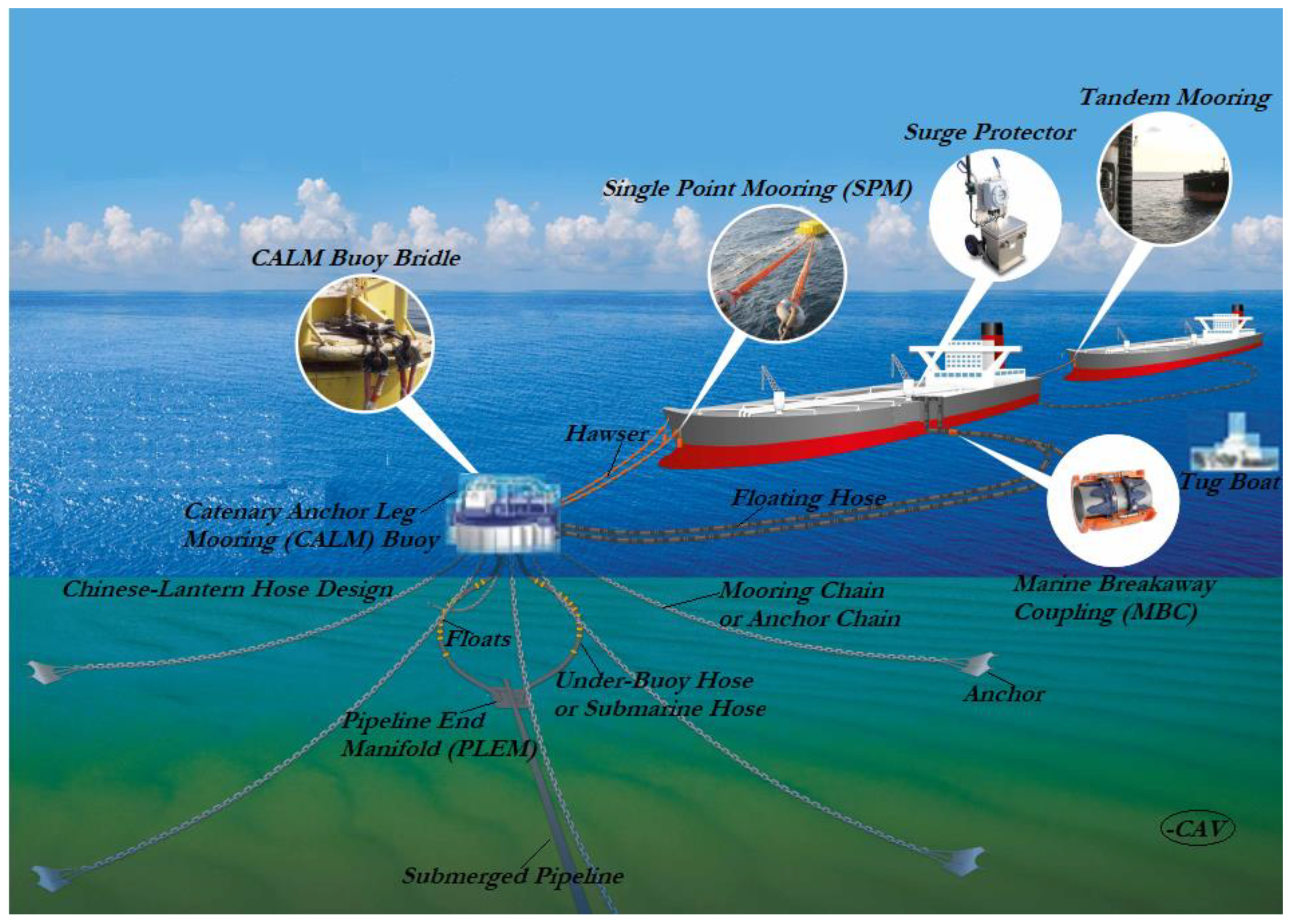
2. Single Point Mooring (SPM): An Overview

A single point mooring buoy is a buoy that is securely anchored to the seabed by several mooring lines/chains/anchors in a permanent position, permitting a liquid petroleum product cargo to be transferred. A bearing system on the buoy allows a portion of it to rotate around the tethered geostatic section. The turntable buoy is a refinement of the bogey wheel buoy (the initial design for an SPM, invented about 1958) that eliminates the rotating frame’s horizontal strain on the swivel bearing. This was accomplished by using a large-diameter three-race roller bearing to support the revolving frame, according to Bluewater ([132,133,134]). A ship can freely weather-vane around the geostatic component of the buoy when it is tethered to this spinning part of the buoy with a mooring link. The SPM system consists of four main components, namely, the body of the buoy, the anchoring and mooring components, the fluid transfer system and the ancillary elements. Static legs linked to the seabed underneath the surface keep the buoy body in place. Above the water level, the body has a spinning portion that is attached to the offloading/loading tanker. A roller bearing, referred to as the main bearing, connects these two portions. Due to this array, the anchored tanker can easily weather-vane around the buoy and find a steady position. The concept of the buoy is determined by the type of bearing utilized and the divide between the rotating and geostatic sections. The buoy’s size is determined by the amount of counter buoyancy required to keep the anchor chains in place, and the chains are determined by environmental conditions and vessel size.

2.1. Categorisation of SPM Moorings

CALM buoy is an application of SPM mooring systems [135,136,137,138,139,140,141,142,143,144]. There are three categories of SPM moorings that will be looked: SPMs, CALM buoys and marine hose systems. These are based on their operational relevance to the CALM buoy system or the connecting FPSO tanker in an SPM unloading or discharging hose system, like deepwater lines, Oil Offloading Lines (OLLs), flexible riser pipes, flexible hoses, and other CALM buoy hose systems [145,146,147,148,149,150,151,152,153,154]. To avoid failure, safety must be key for installation and (un)loading [155,156,157]. An operation to replace or install components can be carried out to change the complete buoy hose system, like on the SBM buoy in Djeno Teminal, Congo [158], as depicted in Figure 2.

Once the floating buoy is secured to the seafloor by moorings, next is the anchoring systems. These might be made up of ships, rigs, piles, or gravity anchors, depending on the local soil conditions. Based on the SPM classification, CALM and SALM are the two most common mooring systems for SPMs. In a CALM system, the buoy is held in place by the CALM’s anchor chain, which runs in catenaries towards anchor points slightly further away from the buoy. The SALM system is similar, with the exception that the SALM is only anchored by one anchor leg. The key advantage of a CALM buoy over a SALM buoy is it is easy to maintain. CALM buoys have been deployed in the vast majority of Marine Terminals since the mid-1990s.

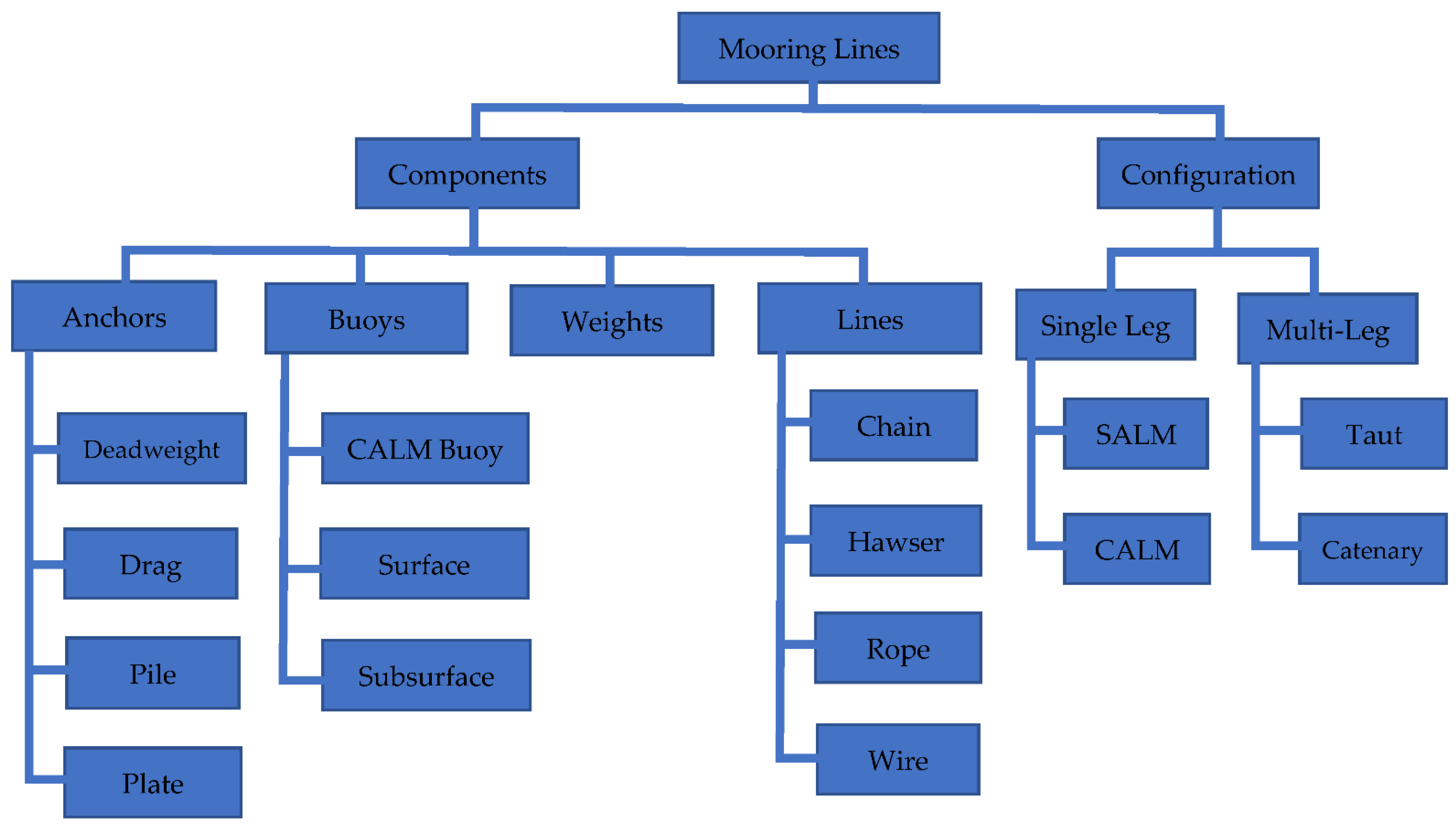
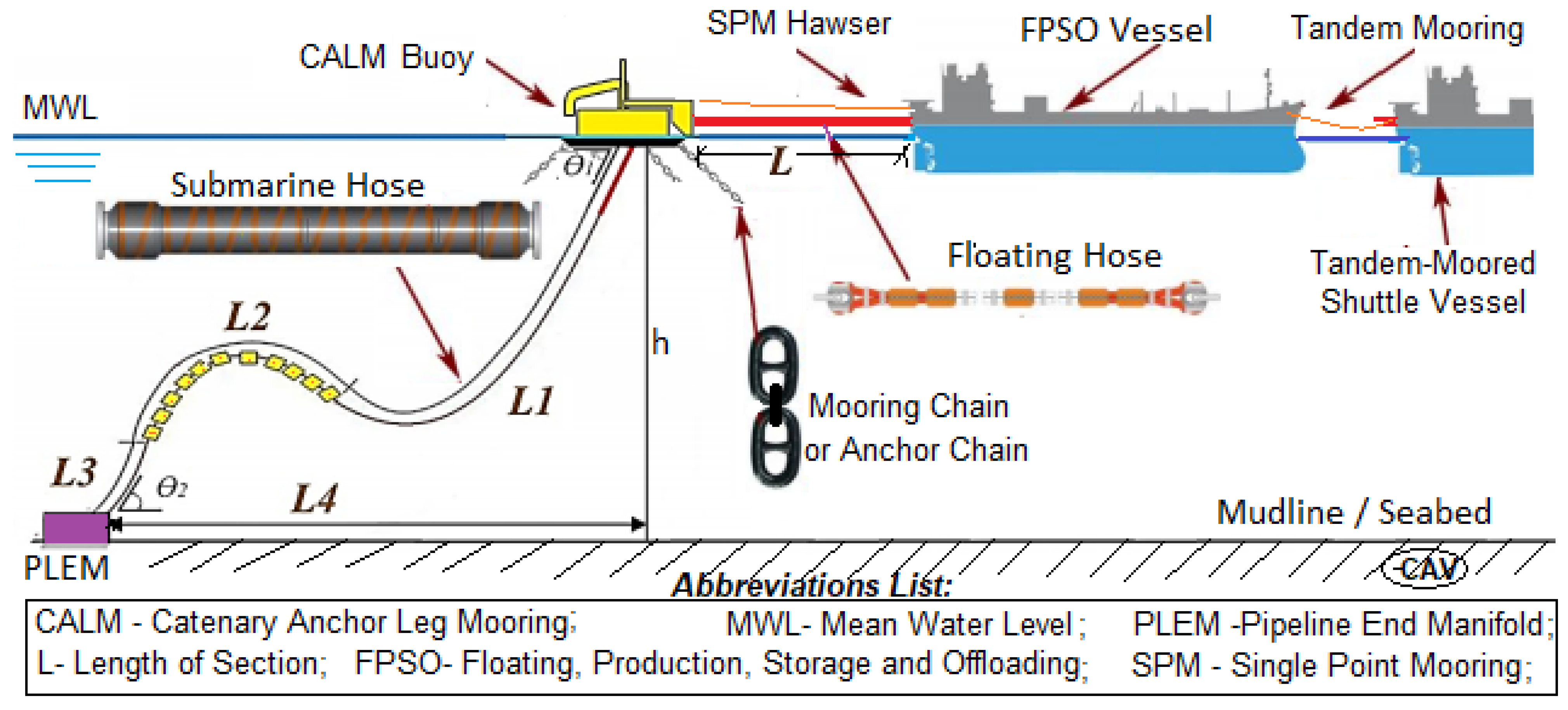
2.1.1. Components of SPM System

Generally, the mooring lines, connectors, and anchors make up a mooring system. The mooring wires can also be used to connect buoys and clump weights. A mooring line can be made of a variety of materials, such as chains, fiber ropes, or wire ropes. Figure 3 represents a CALM buoy system, three mooring configurations and various components, adapted from [159]. The three mooring configurations seen on Figure 3 are the Chinese lantern configuration, single point mooring (SPM), and tandem mooring.

Figure 3 also shows various components like the Marine Breakaway Coupling (MBC), floating hose, under-buoy hose or submarine hose, buoyancy floats, CALM buoy, surge protector, tug boat, submerged pipeline, pipeline end manifold (PLEM), hawsers, CALM buoy bridle, anchor, and anchor chain or mooring chain.

Harnois [160,161] provided a comparison of various mooring line materials. The inertia, elastic stiffness, and damping of a mooring line are affected by the material used. An anchor’s purpose is to secure a mooring line to a fixed place on the bottom. The ability to resist high, horizontal, and in some cases vertical loads in a specific seabed type (soft to hard), cost-effectiveness, and ease of installation are the major requirements for an anchor. There are several types of anchors available, including dead weight, drag embedment, pile anchor, and plate anchor. It is noteworthy to add that the use of hawser is dependent on the size of the vessel to be anchored to the buoy, as hawser systems can use one or two ropes, as depicted in Figure 1, Figure 2 and Figure 3.

A mooring system is made up of many materials and components that are organized in a specific way, as shown in Figure 4. The other SPM components are as follows:

• The access to the buoy deck is provided by a boat landing;
• The buoy is protected by fenders;
• The material handling equipment includes lifting and handling equipment;
• Maritime visibility aids and a fog siren are used to keep moving vessels alert and attentive;
• The navigation aids or other equipment are powered by the electrical subsystem;
• The sources of power systems are batteries and solar systems. While the batteries are replenished on a regular basis, the solar power systems employ sun-sourced renewable energy and maintain the charge in the battery packs, for electrical power;
• A hydraulic system can be added for remote operation with PLEM valves, if needed.

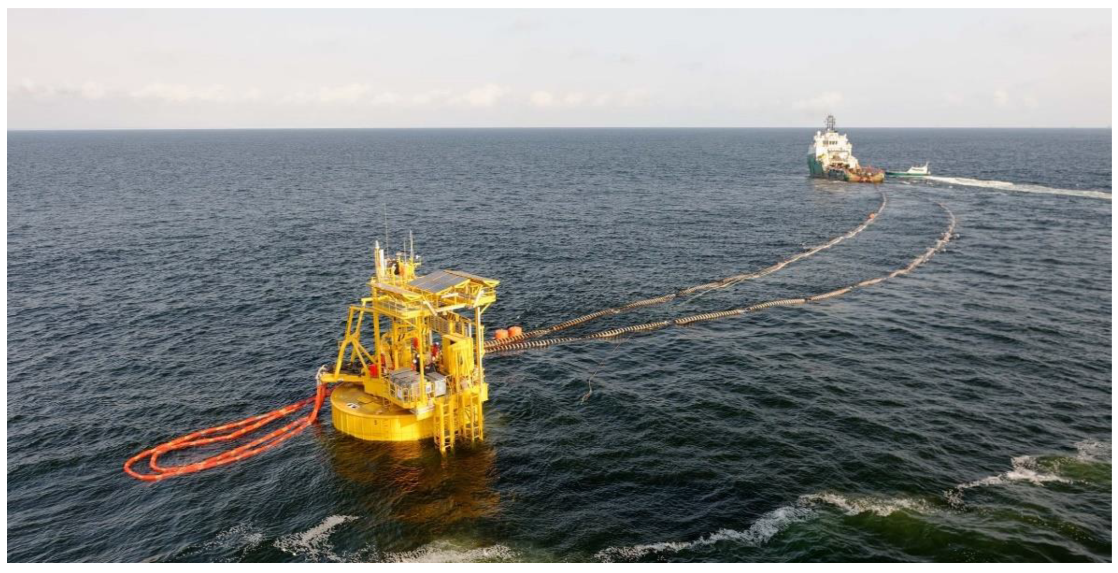
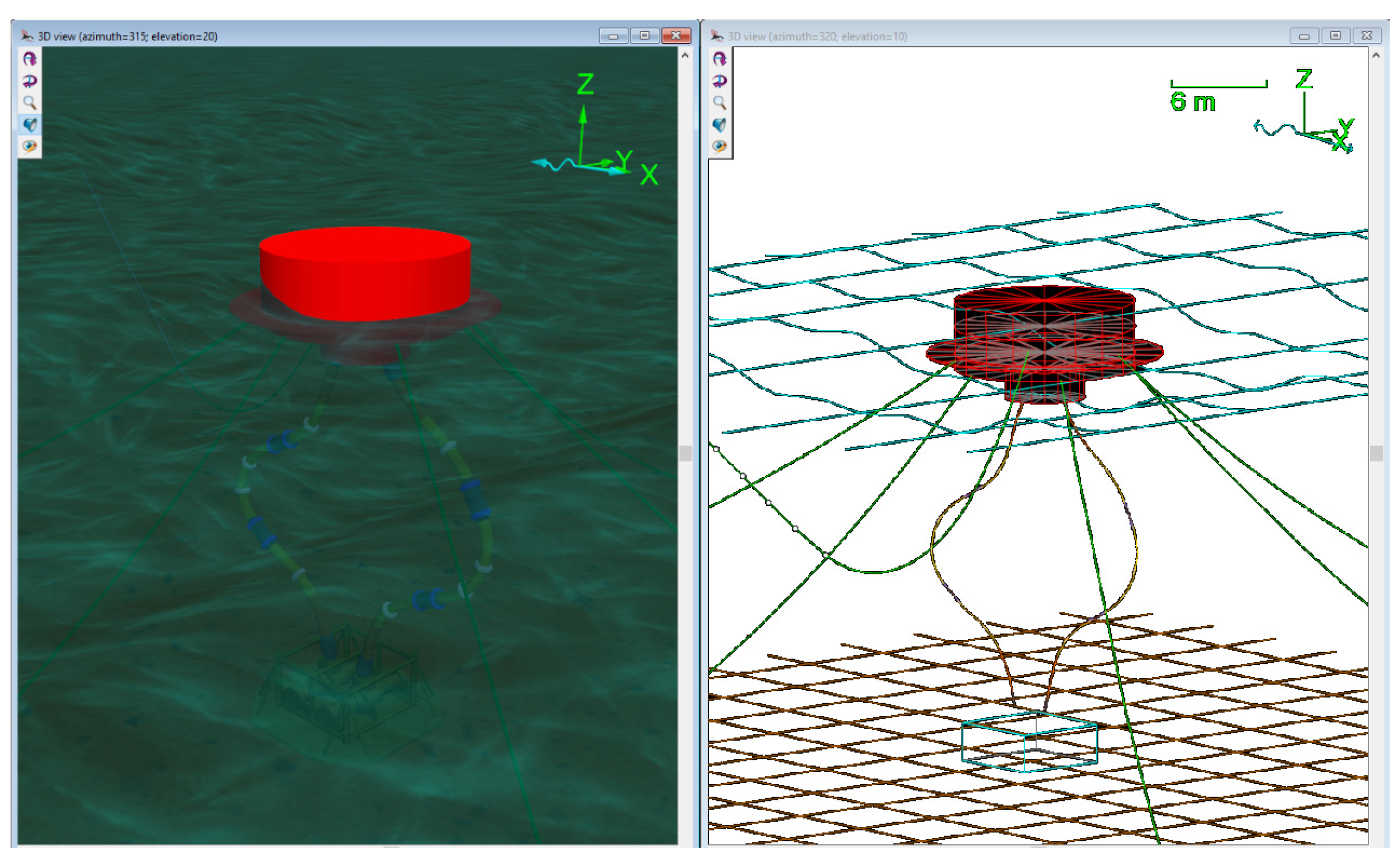
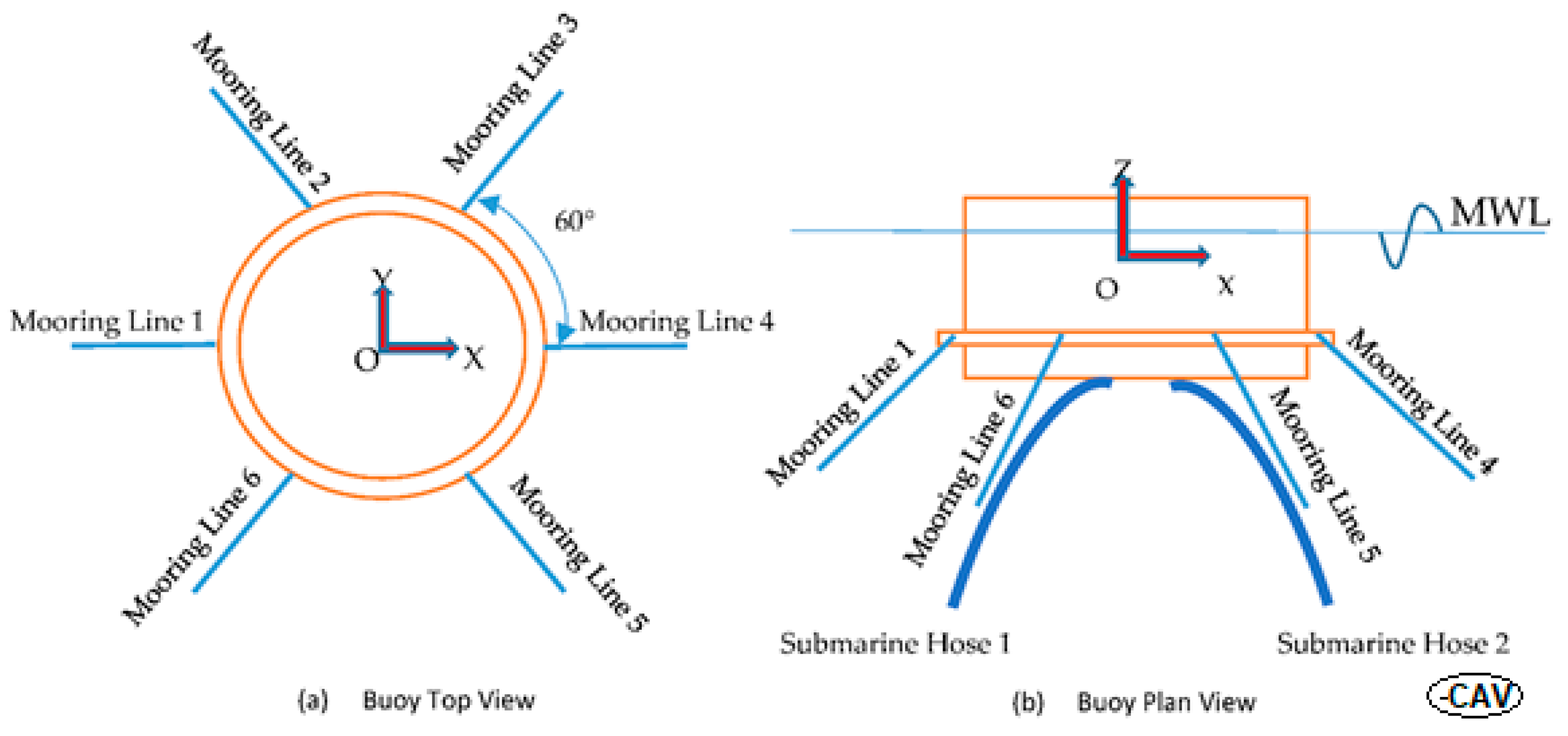
2.1.2. Components of CALM Buoy System

The Catenary Anchor Leg Mooring (CALM) buoy system has a buoy with a pivot, called the turntable. This rotates around the vertical axis of the pivot, as the tanker is moored to it. The floating hose is also connected to the turntable, at an angle through the hose manifold. The elastically moored buoy of radius a is acted upon by a wave train of irregular waves and wave height H progressing in x-direction, as illustrated in Figure 1. The turntable on the mooring buoy can spin around its vertical axis. The tanker is moored to the turntable and is connected to the floating hose strings that are also attached to the turntable. Due to the forces imposed by the currents and waves, the entire system can freely rotate, which is termed weather-vaning. Figure 1 and Figure 3 show Catenary Anchor Leg Mooring (CALM) buoy systems. Basically, there are three CALM system mooring components, namely, the anchors, the chain anchors and the chain stoppers. The anchors are used to hold things together, including the piles or gravity anchors for connecting the seabed with the mooring chain. The most common chain anchors are systems with either six or eight anchor chains. The third component is the stoppers for chains, which are for connecting the buoy with the mooring chains. The anchor chains help to keep the buoy in place. The fluid is transferred to the submarine hose strings via a swivel, which links to the undersea pipeline via the pipeline end manifold.

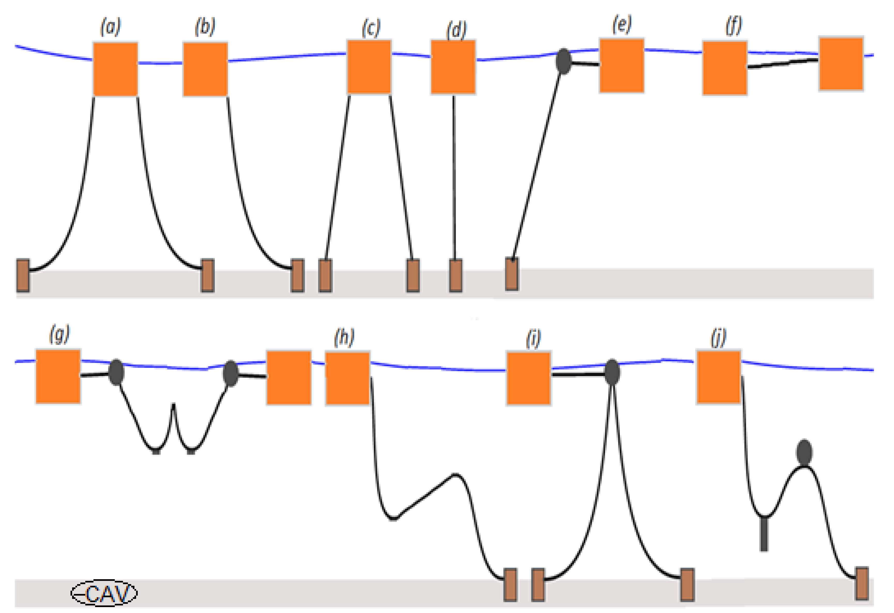
2.1.3. Different Mooring Configuration

There are other types of offshore mooring systems, aside SPM, as summarized in

Table 1. Different categories of moorings for offshore loading systems (Source: [162]).

Category	Description	System Type	Abbreviation	Flexible Hose Type
Articulated	Articulated, buoyant column for rotation. Single seabed attachment, gravity or piled. Mooring by hawser or rigid arm/yoke. Surface flowline connections via floating hoses, or within rigid arm, or aerial hoses from the raised platform (ALC/ALP). Seabed connections via flexible or by universal joint in flowline.	Single Anchor Leg Mooring	SALM	Floating and Submarine
		Single Anchor Leg Rigid Arm Mooring	SALRAM	Floating and Submarine
		Single Anchor Leg Mooring Rigid Arm	SALMRA	Floating and Submarine
		Single Anchor Leg Storage	SALS	SALS use both. ALC, ALP and possibly some SAL designs use universal joints rather than Submarine hoses.
		Articulated loading column	ALC/ARTC
		Articulated loading platform	ALP
Buoy	Buoy has turntable section, or swivel. Seabed fixing by one or more catenary lines or tension legs from varied anchor options. Mooring by hawser or rigid arm/yoke. Surface flowline connections via floating hoses, or within rigid arm. Flexible seabed connections.	Catenary anchor leg mooring	CALM	Floating and Submarine
		Catenary anchor leg mooring—soft yoke	CALM-SY	Floating and Submarine
		Catenary anchor leg—rigid arm	CALRAM	Floating and Submarine
		Rigid mooring buoy	RMB	Floating and Submarine
		Single buoy mooring	SBM	Floating and Submarine
		Unmanned production buoy	UPB	Floating and Submarine
		Vertical Anchor Leg Mooring	VALM	Floating and Submarine
Fixed Tower	Rigid tower/jacket fixed to seabed with above-water rotating section. Mooring by hawser or articulated yoke. Above-water flowline connections by aerial hoses or within articulated yoke. Rigid riser with above-water swivel joint.	Fixed Tower Single Point Mooring	FTSPM	Floating flexibles
		Jacket soft yoke	JSY	Floating flexibles
				Floating flexibles
				Floating flexibles
Floating tower	Large floating tower/spar structure with above-water rotating section. Seabed fixing via multiple catenary lines or tension legs from varied anchor options. Mooring by hawser. Above-water flowline connections by aerial hoses. Flexible Seabed connections.	Exposed location single buoy mooring	ELSBM	Floating and Submarine
		Floating loading platform	FLP	Floating and Submarine
		Floating cylinder facility	SPAR	Floating and Submarine flexibles
Spread	Usually 4 CBM, with hawsers. Flexible risers and surface hose connections.	Conventional (or catenary-anchored) buoy mooring	CBM	Floating and Submarine
Submerged flexible	Flexible riser with pick-up buoy and wire, stored on seabed when not in use; SAL has catenary mooring connection, SLS has none, requiring a DP ship.	Single Anchor Loading	SAL	Floating and Submarine
		Submerged loading system	SLS	Floating and Submarine flexibles
Submerged buoy	Submerged buoy at depth clear of shipping, tethered by one or more catenary lines or tension legs from varied anchor options. Either mooring hawser with pick-up buoy from main buoy, or no mooring connection, requiring DP ship. Flexible or part-rigid (hybrid) riser and flowline connection from seabed, via main buoy to ship, with pick-up buoy and wire. Main buoy usually has swivel/turntable to allow weather-vaning.	Hybrid riser tower	HRT	Floating and Submarine
		Single anchor loading	SAL	Floating and Submarine
		Single leg hybrid riser	SLHR	Floating and Submarine
		Submerged tethered buoy	STB	Floating and Submarine
		Tripod catenary mooring and loading system	TCMS	Floating flexibles
		Ugland Kongsberg offshore loading system	UKOLS	Floating flexibles
Turret	Turret concept involves swiveling manifold integrated with internal well through ship, or external support structure, at bow to allow weather-vaning. Turret may be fixed or disconnectable. Disconnectable turrets submerged with pick-up buoy or on surface. Turret tethered by multiple catenary lines from varied anchor options. Flexible riser from seabed, connection via turret.	Bottom mounted internal turret	BMIT	Floating flexibles
		Buoyant turret mooring	BTM	Floating flexibles
		Riser turret mooring system	RTMS	Floating and Submarine
		Single point turret	SPT	Floating and Submarine
		Submerged turret loading	STL	Floating and Submarine
		Submerged turret production	STP	Floating and Submarine
		Turret riser mooring system	TRMS	Floating and Submarine

. Based on the mathematical modeling, HMs and MMs, considering SPMs for bonded marine hoses, have been developed over 45 years based on earlier works on point moorings and simple floating buoys. The application of offshore hoses has also led to advances in different mooring systems used in fluid transfer, as seen in Figure 5.

Moorings are also applied on shipping vessels for other oil field operations like CO₂ oil recovery [162] as seen in Table 1. Several studies assessed mooring statics and dynamics for CALM buoy, as well as with attached hoses, which were considered as a single point mooring (SPM) terminal [163,164,165,166,167]. The design of each hose-mooring system considers different loadings, predictive motion responses with structural statics/dynamics [168,169,170,171,172,173,174,175,176,177,178], and governing theories on the hydrodynamics of floating structures [179,180,181,182,183,184,185,186,187,188]. In addition, the design of FOS is based on different industry standards [189,190,191,192,193]. The application of a mooring configuration is based on the application requirement, the type of (un)loading operation, and the environmental conditions. Some of these mooring applications require floating, catenary, and reeling hoses, while others require submarine hoses.

2.2. Review on Physical Models on Hoses and SPMs

The selection of hose systems for single point mooring (SPM) systems has been described by Ziccardi and Robbins [194]. Setting up buoys in low-tide areas was discussed as the authors also wanted to stimulate more hose and flexible rubber pipeline designs and applications. They studied the SPM deployments at Tokyo Bay’s Hakozaki and Koshiba terminals. They also included a timeline of hose design and trends. They claimed that the basic designs of under-buoy hoses and floating hoses are comparable. The strong crush resistance of sub-surface hoses, on the other hand, was shown to be dependent on the water depth. This was accomplished by increasing either the wire’s area or the diameter of the helical wire, or both. The rated operating pressure was found to be 5 to 6 times the design burst pressure. They highlighted the abrasion and abuse that the floating hoses attached to the tanker from the buoy were subjected to. They came to the conclusion that developing flexible rubber lines that could sustain high operating pressures and external crush, particularly in severe environments, was critical. The hose system for an SPM terminal was also reliant on both the operational and environmental conditions, according to the report. Physical tests are also used to develop environmental wave spectra, such as the Joint North Sea Wave Project (JONSWAP) wave spectrum and regular wave types like Airy waves [195,196,197,198,199]. Typical recent numerical model of CALM buoy model conducted in Orcina’s Orcaflex by the authors can be seen in Figure 6.

The operational requirements, such as the system’s working pressure, necessitated the transportation of well-specified products with an adequately defined nature. They listed several factors that must be considered when determining the length of hose strings in hose designs, including mean water depth, tide depth (low/high), maximum wave height, buoy position relative to pipeline header, maximum mooring distance, rated working pressure, desired throughput, and product(s) to be transported. They advised that the ultimate design of the under-buoy system should ensure that the hose does not come into direct contact with the seabed of the moored ship under high tide conditions. They looked at the primary design criteria for SPM hoses, underbuoy system, floating hose systems, float sinks, hose designs, and hose diameters, and encouraged greater research from hose manufacturers, using the two case studies that were employed by the US military on unloading from SPM tankers.

Earlier investigations on marine hoses depended on some lengthy calculations and experiments. Brady et al. [200] with the help of Shell B.P Petroleum Company of Nigeria Limited, built a test apparatus that was connected to 60.96 cm (24 inches) hoses attached to a CALM buoy off the coast of Nigeria. A Medilog 4–24 small four-channel cassette recorder, a 4–366 pressure transducer, and a Beaulieu S.P 16 mm Cine camera with a lens width of 5.9 mm were also included in the setup. To measure the strains on the hose of a monobuoy, a strain-gauge measuring spool was installed between the buoy manifold and the first-off buoy hose. They claimed that the hoses closest to the buoy have a lower life expectancy because they carry the majority of the hose stresses. Correlation of the measured loads was achievable using the statistical method described for calculating the 60 s recordings and visual records of the sea conditions. However, this was limited due to a lack of environmental data. Rather than the trial-and-error method employed previously, this technology enabled the investigation of the forces on buoy hoses. They came to the conclusion that the hose problem was primarily caused by fatigue rather than high loads. As a result, increasing the hoses’ strength will improve their performance. SPM terminals were subjected to model testing by Pinkster and Remery [201]. The test results were also used to describe SPM terminal features and hose phenomena found in CALM and SALM mooring systems. They also stressed the need for selecting the appropriate scale for model tests. They cited water depth, the accuracy of the results, and the capacity to generate the needed wave height and period at a certain scale in the basin as critical variables. Water depth, current, wave generators, and wind are some of the variables that can be modified to affect environmental conditions. They also went over the model testing technique, measurements, and analysis in detail. They concluded that nonlinearities were exploited in the construction of the equation of motion, which was then integrated in small time increments step by step. Additionally, based on uncertainties in the prototype’s drag coefficients, the inaccuracies in the estimates of the findings obtained from the model tests due to scale effects should be applied without modification. There was additional discussion of the Pierson–Moskowitz spectrum, wind forces, current forces, first-order wave forces, second-order wave forces, and drag wave drifting equations. However, the methodologies for calculating these forces were not sufficiently developed for design consistency. An industry collaboration with academia was conducted on the feasibility of using geodesic IGW designs for offloading hoses, as reported in Nooij [202]. Another important study that was carried out on the load response of offshore hoses by Lassen T. et al. [203] involved finite element models and full-scale testing for a 20inches-bonded hose with steel end fittings. The study presents limits based on API 17K [204] criteria for the extreme load capacity assessments. The study also included a methodology for predicting the fatigue life of bonded loading hoses’ response to applied bending, tension and pressure using a catenary configuration, with reeling loadings repeated and significantly tensioned. The study emphasized the fatigue life prediction methods, as well as the load impacts on the hose during reeling operations, for both rubber and steel parts.

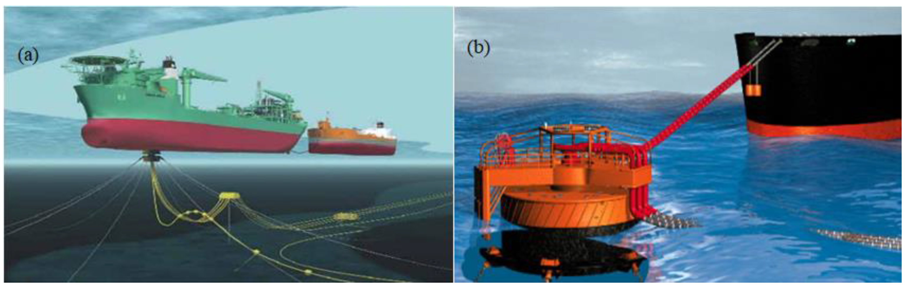
2.3. FPSOs for Marine Hose Operations

There are different types of FPSOs, as summarized (with details on their characteristics) in

Table 2. Characteristics of Turret Moored FPSO and Spread Moored FPSO.

Characteristics	Turret Moored	Spread Moored
Vessel Orientation	360 degree weather-vaning.	Fixed
Environment	Moderate to extreme, multidirectional.	Mild to moderate, one-directional
Field Layout	Fairly adaptable and suitable for a congested seabed.	Not suitable for congested field.
Riser Number and Arrangement	Suitable for medium riser numbers with moderate expansion capabilities.	Suitable for large riser numbers with capability of additional tie-ins.
Station Keeping Performance	Lower number of anchor legs, offset is minimized.	Large number of anchor legs, offset is variable.
Vessel Motions	Motions are reduced as the vessel orients itself into the most suitable environmental direction.	Varies from small to large depending upon the relative direction of vessel and environment.
Riser Connection	Turret provides the connection point for the risers.	Risers hang from the porch on the port/starboard side of FPSO.
Offloading Performance	Better as the FPSO is aligned with the mean environment.	Depends on vessel/environment orientation.
Storage Capacity	Storage is reduced for internal Turret Moored FPSO.	Large storage capacity available.

, that are used in SPMs for transfer, loading and offloading operations. The turret systems are the most common because of their freedom of movement, ease of anchorage, and accessibility during mooring and deployment. A typical turret FPSO in catenary mooring is shown in Figure 7a, and an Offloading FPSO attached to an SPM’s CALM buoy is shown in Figure 7b. A variety of numerical models on other mooring systems can be seen in the literature and existing industry projects on marine hose, as earlier discussed.

3. Model Methodologies and Software Tools

The designs of hose models are considered using some design parameters, as illustrated in Figure 8. Details of these parameters for the mathematical model are given in Section 4 and Section 5. However, these mathematical models are also designed numerically using both commercial and in-house software packages. They are also verified using experimental models. The availability of model tests and numerical simulation tools determines the design of marine hoses, mooring lines, marine risers and other floating structures for deep and ultra-deep waters. The latter has been the subject of various research investigations in the past, leading to the classification of analysis approaches as uncoupled, completely coupled, or hybrid, as in the following sections.

3.1. Uncoupled Methodology

This was the traditional method for analyzing mooring lines and risers, which involved numerical tools based on uncoupled formulations. In general, this approach starts with motion analyses, where mooring lines and risers are represented by simplified models (e.g., scalar coefficients), and vessel motions are calculated in terms of static offsets, as well as wave frequency (WF) and low frequency (LF) components. In a second stage, those offsets and motions are used as input for structural studies of the lines modelled by finite element (FE) meshes. Typically, such studies are carried out for each individual riser. The fundamental benefit of the uncoupled techniques is that each simulation has a cheap processing cost. However, they have significant, well-known flaws that could result in significant inaccuracies in deep-water circumstances and Floating Production systems (FPSs) with a large number of risers. Such flaws were identified by [205,206,207,208,209], addressing the following topics:

(1)

The uncoupled approach does not normally account for mean current loads on moorings and risers, but in those scenarios, the interactive effects of current forces on the Submarine elements and the mean offset and LF motions of the floater are significant;

(2)

A significant damping effect of the moorings and risers on LF motions must be included in a simplified way, usually as linear damping forces. Because multiple characteristics are involved, creating simplified models of this event is difficult. It should be noted that this classification of “uncoupled techniques” could include a variety of analysis methodologies.

Based on the classification, the fundamental or “classic” uncoupled technique can be described in two ways:

(a)

Uncoupled formulations utilized in the numerical tools deployed in the analysis of the floating structures, in which the vessel’s hydrodynamic response is unaffected by the lines’ nonlinear dynamic behavior;

(b)

The analytical technique takes into account the low or negligible integration for both the hose risers and mooring systems.

It is vital to distinguish between these two features because, even when only uncoupled programs are available, some amount of integration for both hose risers and moorings is achievable using variations on the “traditional” uncoupled methodology. These enhancements, which have been applied for over 25–35 years, include the use of improved algorithms for determining the scalar coefficients used in the vessel’s motion equations to describe the behavior of these lines. Even these refinements contain a number of limitations. They do not capture the non-linear dynamics and their interplay in both the lines and vessel completely. This includes the nonlinearity obtained in the response of the damping of the sections that control the vessel’s low-frequency (LF) motions. When the water depth increases, this fluid–structure interaction (FSI) increases its impact and has additional relevant effects, thus it could yield unreliable results and erroneous outputs for these deep-water scenarios.

3.2. Coupled Methodology

Using coupled analytical tools is the most accurate approach for considering the interaction between the components of an FPS and properly predicting the individual responses of the vessel, mooring lines and hose risers. In general, such tools use a time-domain solution method and a rigorous representation of the lines using FE models, taking into account any nonlinearities in the system’s dynamic response. In the literature [210,211,212], descriptions of different coupling formulations investigated for the fully coupled analysis of FPS (referred to as “weak coupling” WkC and “strong coupling” StC) have been presented. The WkC formulation focuses on the hull equations of motion: forces operating on the right-hand side of the hull equations perform the coupling between the hydrodynamic model of the hull and the hydrodynamic/structural model of the lines. The finite element mesh of all moorings and hose risers is integrated into a single set of equations in the StC formulation, and the hull is regarded as a “node” of this model. Only coupled analytical tools can simultaneously produce vessel motions and detailed structural responses of the mooring lines and risers, resulting in a “completely coupled technique.” The mooring lines and hose risers should be represented with a finite element mesh fine enough to precisely establish all key features of the structural response for this purpose (not only their top tensions, but also, for instance, tensions and moments near the touch-down zone). However, this may result in high computational costs for fully coupled analysis tools; in any case, emphasizes the importance of performing fully coupled analyses for at least some critical cases, or for specific studies wherein small-scale tests are not possible due to the limited depth in wave tanks.

3.3. Hybrid Coupled Methodology

Although devising alternate solution methods and algorithms to minimize the computer costs of coupled analyses (e.g., optimized time-domain methods with adaptive time-step variation, or frequency-domain methods) is an important line of research, the goal of achieving a balance between accuracy and computational efficiency has also been sought by proposing “hybrid” analgesics. This classification can include a variety of procedures, such as “coupled motion analyses” and “semi-coupled analyses”, which will be discussed next. Since these hybrid processes may be distinguished by the use of coupled models that introduce simplifications or approximations, they shall be referred to as “simple coupled analyses” from here on.

3.3.1. Coupled Motion Analysis

This is a two-step technique for analysis, as shown in Figure 8. The first phase (the “coupled motion analysis” itself) uses a coupled model with FE meshes that are coarser than those used in fully coupled analyses. The meshes are created to accurately represent the hose risers’ overall contribution in terms of top tensions, mass, and damping (therefore considering the non-linear dynamic interaction between vessel and lines). As a result, their vessel motions are more precise than those obtained from uncoupled motion analyses. With lower processing costs, the accuracy is comparable to that of fully coupled analyses. The detailed structural response of the hose risers (e.g., tensions and moments near the touch-down zone) is obtained in the second step of the procedure, which consists of prescribing the motions at the tops of the uncoupled FE models of each individual riser, now modeled with more refined meshes to obtain these results. Reviews of marine risers provide a more extensive overview of the approximations and benefits of this technique [123,124,125,126,127].

3.3.2. Semi-Coupled (S-C) Motion Analysis

This is a three-step technique for analysis. In the first phase, a coupled model (similar to the one described in Section 3.3.1) is used to perform a nonlinear static analysis with the static components of the loadings, yielding the system’s mean equilibrium position. Other static studies begin with the static equilibrium configuration in the second step, using modest values of prescribed displacements at the platform’s center of gravity (CG) for each of the six rigid-body DoFs. An equivalent 6DoF global stiffness matrix is calculated from the acquired comparable forces, representing the global contribution of all mooring lines and hose risers. This comprises a linearized tangent stiffness matrix around the static equilibrium configuration. Finally, an uncoupled dynamic analysis of the platform is performed, in which only the 6DoF vessel equations of motion are solved, and the equivalent global matrix is added to the platform’s hydrostatic matrix. From the perspective of the lines, this technique is quasi-static, yielding conclusions that are not as stringent as those obtained from a completely coupled analysis, but they are more accurate than those obtained from a standard uncoupled formulation (in which the lines are represented by scalar models or catenary equations). The equivalent stiffness matrix of the lines is calculated using a full FE model, allowing it to be evaluated for a wide range of complex line configurations, including effects that are typically overlooked by traditional quasi-static scalar formulations, such as the influence of current loads along the lines, the coupling of two or more lines, and bending moments when the lines bend. The inertial and damping contributions of the lines can be integrated to increase the precision of the platform motions supplied by this S-C method by computing equivalent global six-DOF matrix coefficients for its mass and damping. Numerical decay tests can be used to achieve these calculations, when the primary goal of analysis is to observe the motion response.

3.4. Software Packages

Based on the mathematical model of marine hoses, marine risers and mooring lines, there are different types of software packages that can be applied, as summarized in

Table 3. Marine Hose, Marine Riser and Mooring Analysis Software. [Note: Asterisk (*) is author’s star rating based on popularity and usage of the software; where 5* is highest, while 1* is least).

Software	Vendor	Approach			Academic Availability at LancsUni	Popularity	Usage
		Nonlinear FEM	Frequency Domain	Time Domain
Orcaflex	ORCINA	√	√	√	√	****	Wide
ABAQUS	SIMULIA	√	√	√	√	*****	Limited
ANSYS	ANSYS	√	√	√	√	*****	Limited
DeepLines	PRINCIPIA	√	√	√		***	Limited
ANFLEX	-	√	√	√		***	Limited
Freecom	MCS	√	√			*	Limited
Flexcom	MCS	√		√		*****	Wide
Riflex,	MARINTEK	√	√	√		*****	Limited
Simscale	SIMSCALE	√		√	√	***	Limited
Sesam	DNV	√	√	√		***	Limited
Orcalay	Orcina	√	√	√		***	Limited
Pipelay	MCS	√	√	√		***	Limited
Solidworks	Dassault Syst.	√	√	√	√	*****	Limited
Mathcad	MATHSOFT	√	√	√		****	Limited
MatLab	MATHWORKS	√	√	√	√	*****	Limited
PVI	Pegasus Vertex	√	√	√		*	Limited
MOSES	Bentley	√	√	√		****	Wide
DeepC	DNV	√	√	√		****	Limited
Helica	DNV	√	√	√		**	Limited
LabView	National Instru.	√	√	√	√	****	Limited
PIPESIM	Schlumberger	√	√	√		*	Limited
OLGA	Schlumberger	√	√	√		*	Limited
Inventor	Autodesk	√	√	√	√	***	Limited
VIVANA	DNV	√	√	√		****	Limited

and

Table 4. Mathematical Modeling Software Packages for Mooring and Catenary Systems.

Software	S	QS	TD	FD	WEC	CALM	SPM
Commercial:
- OrcaFlex [213,214]	x		x		x	x	x
- AQWA [215,216,217]	x	x	x	x	x	x	x
- DNV Sesam						x	x
* Deep C [218]					x	x	x
* MIMOSA [219]	x			x	x	x	x
* RIFLEX [220]			x			x	x
* SIMA [221]					x	x	x
* SIMO [222]
- FLEXCOM [223]	x	x	x	x	x	x	x
- Proteus DS [224]			x		x	x	x
Open-source:
- MAP [225]		x
- MoorDyn [226]			x			x	x
In-house:
- AQUA-FE			x			x	x
- MoDEX [227]			x			x	x
- MooDy [228,229]			x			x	x
- WHOI Cable [230]	x		x			x	x

Note: CALM means Catenary Anchor Leg Mooring, SPM means single point mooring, WEC means Wave Energy Converter, S is static, QS is quasi-static, TD is time-domain, FD is frequency domain. Source: [66].

. There are different types of riser analysis software that can be applied in both the riser-specific and general-purpose software packages currently available. Table 3 discusses the most widely used riser software and its availability for this research at Lancaster University (denoted as LancsUni). Table 4 is also discusses different software that are applicable for the design and analysis of various mooring systems. This is detailed in the body of the paper, with more discussion of their formulation, governing equations and bounding theories. This section presents different software packages and their applications. For instance, Orcaflex ([213,214]) has been applied on different offshore applications, from pipelaying, reeling, loading hoses to subsea lifting operations.

4. Mathematical Model and Other Model Types

Different theories related to the hydrodynamics and statics of bonded marine hoses attached to a CALM buoy have been proposed, as presented in this section. Since these hoses are high-pressure, high-temperature (HPHT) structures, it is important to also discuss some of the mathematical background of the test methods for the hoses.

4.1. Theory Formulation

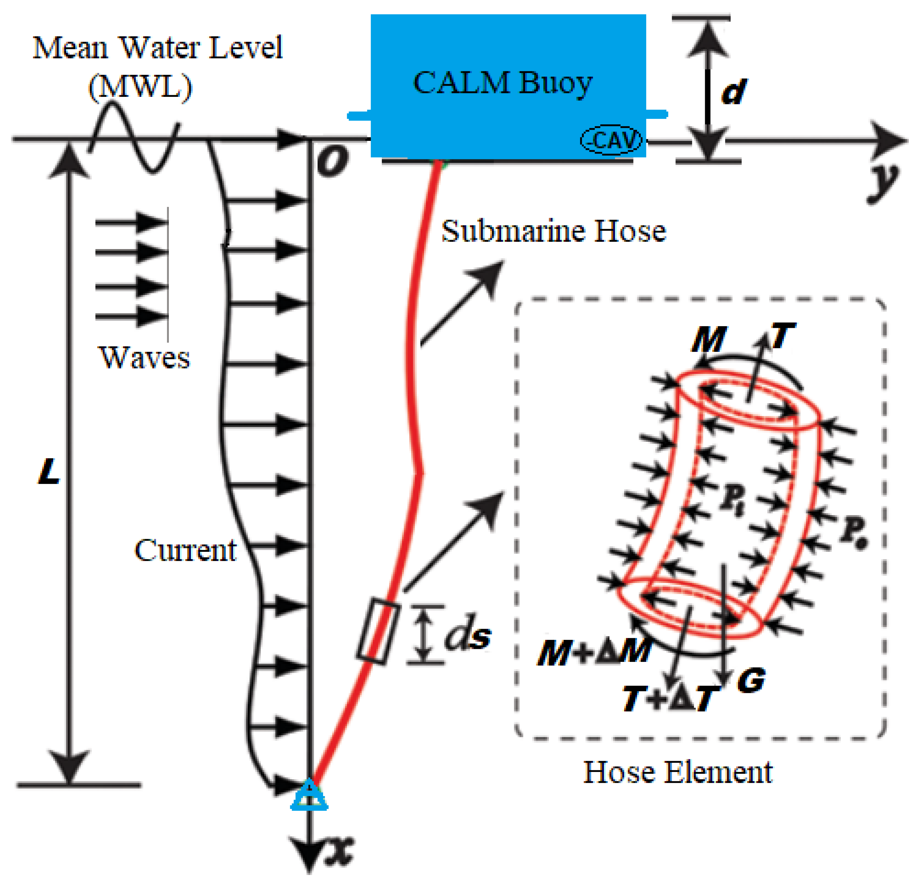
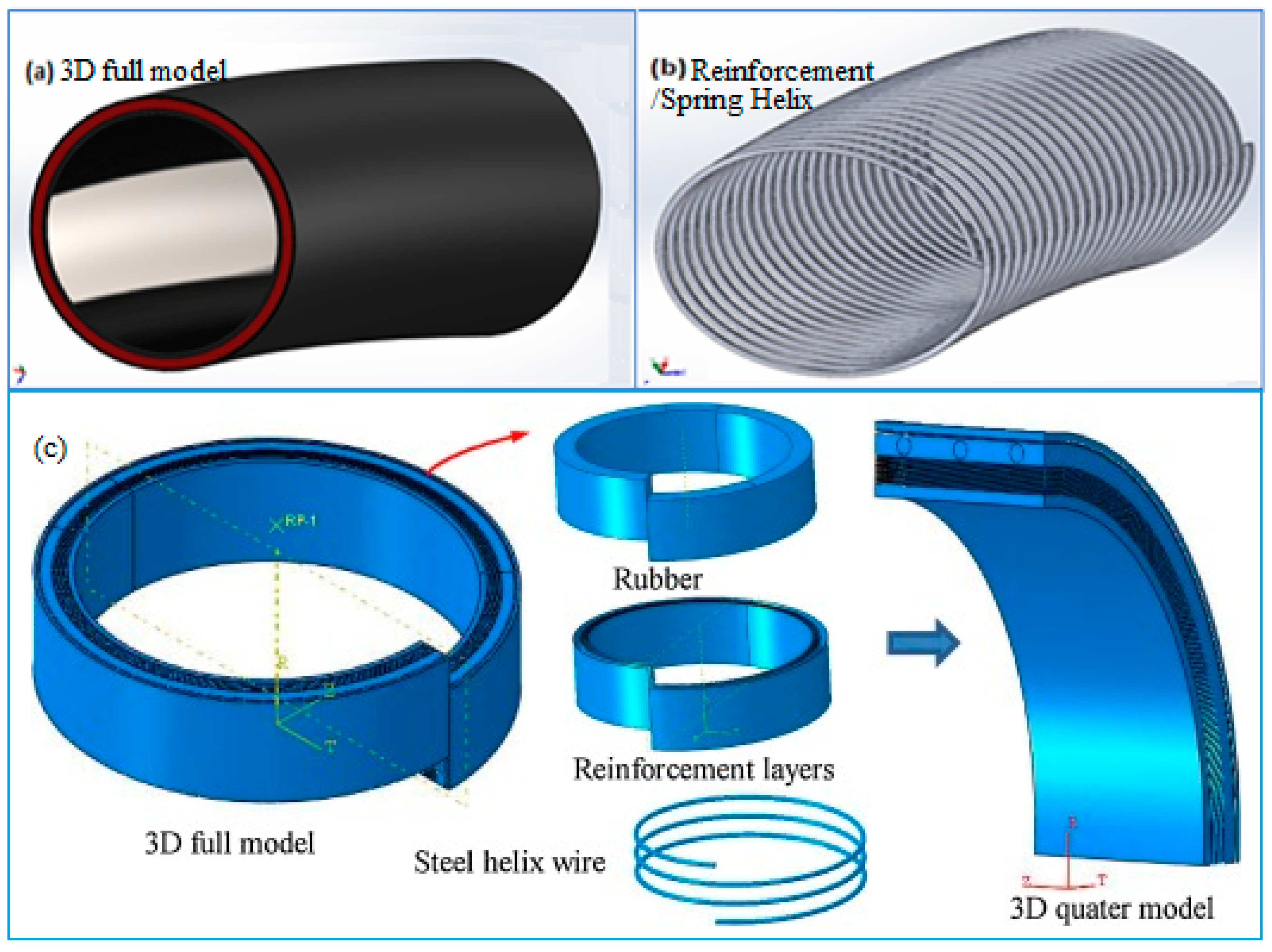
4.1.1. Mathematical Formulation of Hose Model

Based on the given problem, the mathematical formulation of the hose model was developed with some simplifications, based on the experimental findings of the author and some experiences reported in offshore engineering practice. These applications can be seen on moored WECs [231], steel catenary risers [232,233,234,235,236,237,238], flexible risers [239,240] and pipelaying operations [241,242,243,244,245]. The seabed considered is a horizontal and a rigid plane, and the material for the hose is isotropic and in an elastic state. The marine environment for this mathematical model is a stable environment. To simplify the model, the contact points of the pipeline to the pipeline end manifold (PLEM) are not considered; however, the tension at hose ends is considered. The frame of reference is the Cartesian coordinate system (CCS), with the origin shown in Figure 1. This is the locus at which the pipeline meets the seabed, called the touch-down point (TDP). The natural coordinate system for the model is established along the hose string. It is also noteworthy that the arc length of the hose string, s, determines the physical properties of the submarine hose string.

Considering the wave–structure interaction, the Laplace Equation is used to formulate the equation governing the motion. This is derived from the Continuity Equation for fluids, as shown in Equation (1).

$$\frac{\partial u}{\partial x}+\frac{\partial v}{\partial x}+\frac{\partial w}{\partial x}=0$$

(1)

The motion of the system can be represented by Equation (2). This presents the Newtonian force, F, derived from the external load of the system as the sum of the inertia force of the system, the viscous damping load and the elastic force components (also called the stiffness load of the system).

$$F=Ma+Cv+kx$$

(2)

For incompressible flow, as considered here, the Continuity Equation applies, wherein the components of the flow domain are denoted by u, v and w.

$${\nabla }^2\varphi =\frac{{\partial }^2\varphi }{\partial r^2}+\frac{1}{r}\frac{\partial \varphi }{\partial r}+\frac{1}{r^2}\frac{{\partial }^2\varphi }{\partial {\theta }^2}+\frac{{\partial }^2\varphi }{\partial z^2}=0; for a\le r\le \infty ;-h\le z\le \eta ;-\pi \le \theta \le \pi$$

(3)

For an irrotational motion, all the vector components of the rotation are equal to zero. Thus,

$$(\frac{\partial w}{\partial y})-(\frac{\partial v}{\partial z})=0;(\frac{\partial u}{\partial z})-(\frac{\partial w}{\partial x})=0;(\frac{\partial v}{\partial x})-(\frac{\partial u}{\partial y})=0$$

(4)

For simplicity, let us denote the vector components in the Cartesian coordinates as $u=\frac{\partial \varphi }{\partial x}, v=\frac{\partial \varphi }{\partial y}, and w=\frac{\partial \varphi }{\partial z}$, where the scalar functions $\mathsf{\phi }$(x,y,z) are the relations used in Equation (4).

Introducing the function ϕ to the Continuity Equation gives the second-order linear differential equation, called the Laplace Transform, as given in Equation (5).

$${\nabla }^2\varphi =\frac{{\partial }^2\varphi }{\partial x^2}+\frac{{\partial }^2\varphi }{\partial y^2}+\frac{{\partial }^2\varphi }{\partial z^2}=0$$

(5)

Where $\nabla$ is the Laplace grad operator, u is the velocity of the fluid and the motion of the fluid can be expressed as $\nabla \mathrm{u}=0$ based on Laplace formation. Thus, in a plane coordinate system, the Laplace Equation is given by the relation:

$${\nabla }^2\varphi =\frac{1}{r}\frac{\partial }{\partial r}\left(r\frac{\partial \varphi }{\partial \theta }\right)+\frac{1}{r^2}\frac{{\partial }^2\varphi }{\partial {\theta }^2}=0$$

(6)

For the conventional cylindrical coordinate or polar coordinate (r, θ, z), the Laplace Equation is given as Equation (7),:

$${\nabla }^2\varphi =\frac{{\partial }^2\varphi }{\partial z^2}+\frac{1}{r}\frac{\partial }{\partial r}\left(r\frac{\partial \varphi }{\partial \theta }\right)+\frac{1}{r^2}\frac{{\partial }^2\varphi }{\partial {\theta }^2}=0$$

(7)

For a buoy of radius a and height L, the bounding surface is r = a and the two flat parts are z = 0 and z = L. Thus, the boundary conditions can be depicted by the following for the given function, called the Velocity Potential, ϕ(r,θ):

$$\begin{gathered} \varphi \left(r,\theta ,0\right)=0; \\ \varphi \left(a,\theta ,z\right); \\ \varphi \left(r,\theta ,L\right)=\varphi \left(r,\theta \right) \end{gathered}$$

(8)

4.1.2. Assumptions

The buoy system is considered to comprise the buoy, the mooring cables and the connected submarine hoses. For this study, the hawser lines and the floating hoses are not included, as the responses from other FPSO and transport vessels are not considered. The buoy is also considered as a single-system rigid body with 6DoFs, as shown in Figure 1. The following is assumed:

• The fluid is incompressible, irrotational, and bounded by the surface of the buoy, the rigid bottom and the free surface;
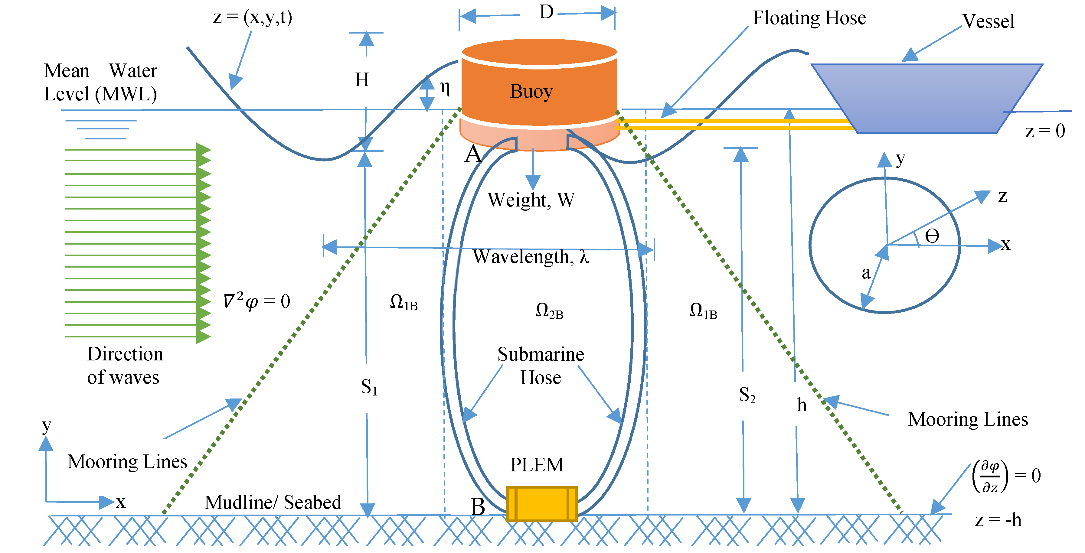
• The seabed is horizontal and on a rigid plane. For the diffraction analysis, the fluid motion is in a cylindrical coordinate system of form (r, θ, z);
• The submarine hose is considered as a beam undergoing pure bending;
• The internal and external forces will place longitudinal forces on the hose. However, the effects can be negligible at depths with small effects;
• The hose curvature is the inverse of the minimum bend radius (MBR), and the curvature calculation can be approximated using $\frac{1}{r}=\frac{{\partial }^2\mathrm{z}}{\partial {\mathrm{x}}^2}$. The measurement of the bend radius of the hose is never less than the MBR;
• The influences of both the horizontal forces and the shear forces on the curvature are negligible, depending on the bending moment;
• Due to some nonlinearities within the hose geometry, there will be some nonlinearities in the motions of fluids within the hose;
• The hose is considered to possess a solidly rigid body with constant bending stiffness for all given cross-sections transverse to the axis of the hose. The hose also transports (or carries) fluid under high pressure, and the fluid can be oil or water;
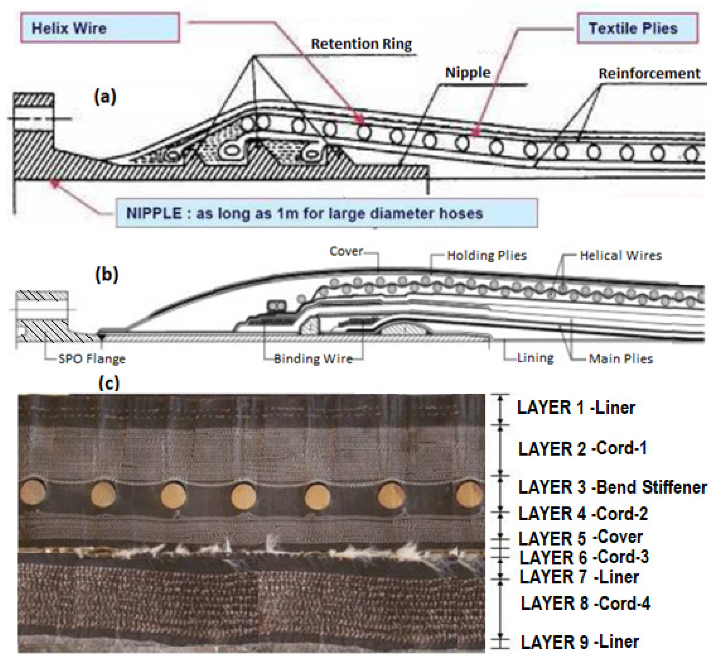
• The hose can be made of different sections, flanges, reinforced ends, floated sections and unfloated sections, and can have different section radii. A uniform density of the hose is assumed for both the rubber and steel sections.

4.1.3. Boundary Condition Formulation

The boundary conditions for the system are formulated with some assumptions in Section 4.1.2, as discussed herein. Illustrations of one (1) floating hose connected between the floating buoy and the FPSO, and two (2) submarine hoses connected underneath the buoy in a Chinese lantern configuration (with environmental forces on the system, such as waves), are shown in Figure 1. The buoy is cylindrical in shape and the submarine hoses are connected to the seabed by a fixed connection to the pipeline end manifold (PLEM). The seabed is assumed to be a horizontal plane. For simplification in modeling this system, a free-floating buoy was utilized. As such, in the initial boundary condition formulation, the mooring lines are not considered. Potential theory is used in the formulation of the boundary conditions, as given herein. The motion of the system is based on Equation (1), which is the Laplace Transform derived from the Continuity Equation of fluids. The following boundary conditions (represented as a–f) are related to Equation (2):

(a)

Dynamic boundary conditions:

$$\frac{\partial \varphi }{\partial t}+g\eta +\frac{1}{2}\left\{{\left(\frac{\partial \varphi }{\partial r}\right)}^2+{\left(\frac{1}{r}\frac{\partial \varphi }{\partial \theta }\right)}^2+{\left(\frac{\partial \varphi }{\partial z}\right)}^2\right\}=0; for r\ge a; z=\eta (x,y,t)$$

(9)

(b)

Kinematic boundary conditions:

$$\frac{\partial \eta }{\partial t}+\left(\frac{\partial \varphi }{\partial r}\right)\left(\frac{\partial \eta }{\partial r}\right)+\frac{1}{r^2}\left\{\left(\frac{\partial \varphi }{\partial \theta }\right){\left(\frac{\partial \eta }{\partial \theta }\right)}^{ }\right\}=\frac{\partial \varphi }{\partial z}; for r\ge a; z=\eta (x,y,t)$$

(10)

(c)

Free surface boundary conditions:

$$z=\eta \left(x,y,t\right)$$

(11)

$z=\eta \left(x,y,t\right)$ represents the free surface [246]. The free surface boundary conditions are given in Equations (6) and (7), which are to be satisfied by both the wave elevation η and velocity potential ϕ.

(d)

Body surface boundary conditions:

$$\frac{\partial \varphi }{\partial r}=0; for r=a;-h\le z\le \eta$$

(12)

(e)

Seabed (or bottom) boundary conditions:

For an impermeable seabed of depth h(x,y), carrying a floating buoy, the seabed boundary condition is given by Equation (13);

$$\frac{\partial \varphi }{\partial z}=0; for z=-h$$

(13)

(f)

Radiation boundary conditions:

With the assumption of infinity, the radiation boundary condition is given by Equation (9), where ϕ_S denotes the scattered wave potential for this condition and ϕ_I denotes the incident wave potential.

$$\varphi (r,\theta ,z,t)=Re[\varphi \left(r,\theta ,z\right)e^{i\sigma t}]=Re\left[\right({\varphi }_I+{\varphi }_S\left)e^{i\sigma t}\right]$$

(14)

Thus, Equations (15) and (16) will satisfy the radiation potential at infinity;

$$\underset{kr\to \infty }{\lim }\surd kr\left(\left(\frac{\partial }{\partial r}\right)\pm ik\right){\varphi }_s=0; i=\surd -1$$

(15)

$$\underset{kr\to \infty }{\lim }\sqrt{kr}\left(\left(\frac{\partial }{\partial r}\right)\pm ik\right)\left({\varphi }_{ }-{\varphi }_I\right)=0; i=\surd -1$$

(16)

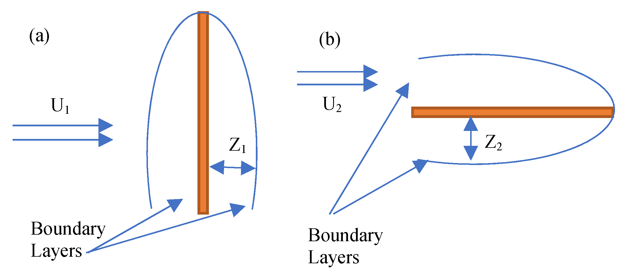
4.1.4. Boundary Layer

The boundary layer for the flow around the hose line attached to a CALM buoy can be idealized using a beam with a uniform cross-section, acted upon by velocities U₁ and U₂, as shown in Figure 9. At initial conditions, the hose is stationary and the flow around it is assumed to be stationary. To formulate the boundary value problem (BVP), the wave potential theory was considered with grouped set equations for the boundary conditions presented in Section 4.1.3, following Lighthill’s approach ([247,248]), which was based on the Laplace Equation. The coordinate systems are those used in Figure 1, where XYZ is the CCS with a z-axis facing upward, and X-Y coincides with the axis acting across the free surface that is unperturbed. The fluid domain is not limited in the horizontal position. The seabed is also rigid and horizontal, and Equation (13) is valid for the z-axis. The total velocity potential for the system is given by Equation (18). This includes the incoming wave on both the hoses and the CALM buoy, as considered in the wave mechanics of HM-MM systems.

We used these following definitions:

$$V_r=\frac{\partial \phi }{\partial x}; V_{\theta }=\frac{1}{r}\frac{\partial \phi }{\partial \theta }; V_z=\frac{\partial \phi }{\partial z}$$

(17)

where g is acceleration due to gravity, h is the water depth below a mean water level, ϕ is the total velocity potential, ${\varphi }_s$ is the scattered wave potential, ${\varphi }_I$ is the incident wave potential, η is the height of the free surface, a is the radius of the buoy, k is the wave number, T is the wave period, C is the wave celerity and λ is the wavelength.

$$\varphi ={\varphi }_I+{\varphi }_s$$

(18)

The wavelength, λ, the wave number function (called the wave celerity, C) and the wave period, T, are set as in the equations C = λ/T and $k =2\pi /\lambda$ [249,250,251,252,253,254,255]. Slender bodies such as risers, hose strings, piles and mooring lines make second-order wave loading contributions to the flow domain. Discussions on the effect of the theory on large vertical cylinders are available in the literature [181,182,183]. In principle, these properties contribute to the behavior of the structure in water or an ocean body. Equations (15) and (16) are derived from the perturbation series expressions for higher-order corrections, with Taylor series expansion.

For submarine hoses, the effect of the wave’s action on the buoy motion and the hoses is considered during the design of the manifold and the connections. This helps the hose string to withstand the minimal horizontal movements made by the buoy [256,257]. The initial displacement of the hose under static conditions is denoted by Y₀, the displacement at equilibrium is denoted by Y_e and the sloped angle the hoses make with the manifold of the buoy underneath is θ₀. At equilibrium, the stresses experienced by the hoses of the buoy are not dependent on the stresses experienced at the PLEM connection. However, there must be a sufficient length of hose string from the buoy to the PLEM.

Thus, the boundary condition at the buoy is given by Equation (19):

$$x=0; y=y_0; \theta ={\theta }_0$$

(19)

While the boundary condition at the hose end is given by Equation (20):

$$x=h; y=y_{e }; \theta ={\theta }_0$$

(20)

Another condition that is considered in the BVP is the fluid domain, as in Equation (21):

$$\Delta \varphi =0$$

(21)

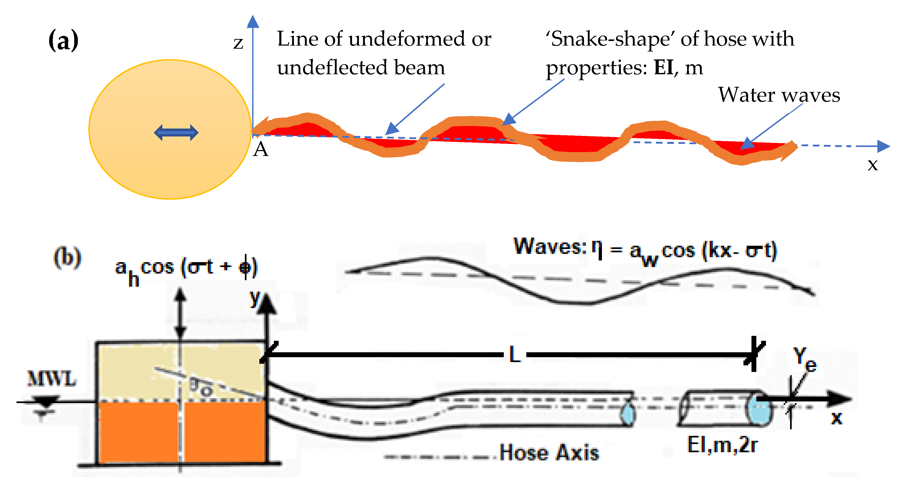
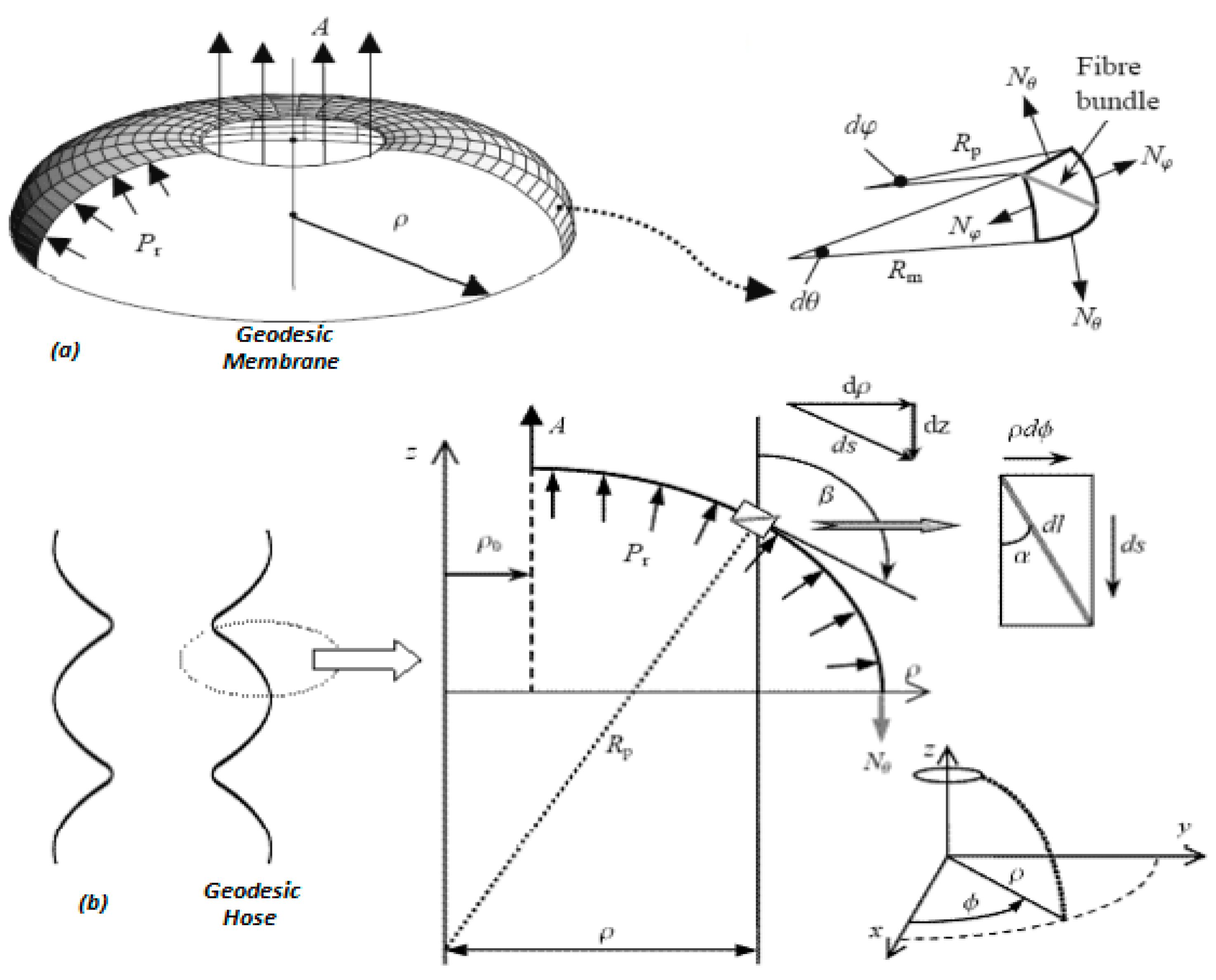
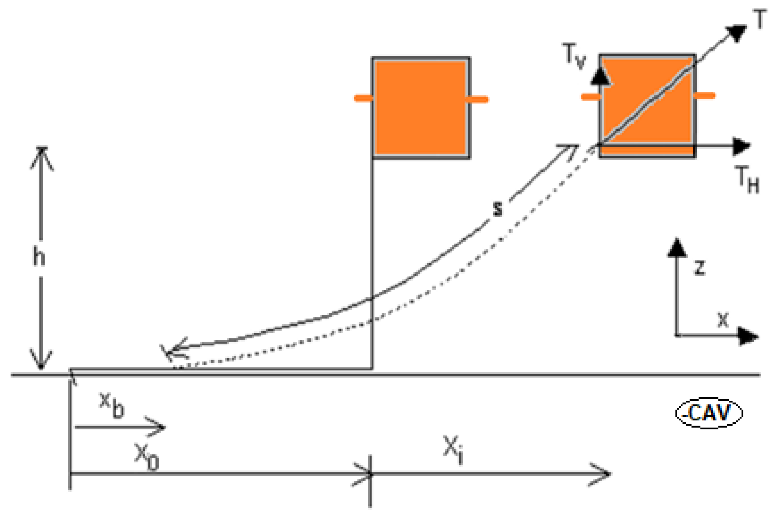
4.1.5. Modeling the Submarine Hose

For this system, there are nonlinearities in the buoy system. These include the points of connection on the buoy for both the riser hoses and the mooring lines, the different materials used in the hose sections, and the wave trains for the irregular waves acting on the system. There are also nonlinearities in the free surface under the boundary conditions, presented via Equations (22) and (23), which are a result of the wave form, the current and the propagating waves.

Consider the submarine hose string depicted in Figure 10, with hose radius r and length S. The different sections of the hose string are designed differently. The front sections of the hose, connected to the manifolds on the buoy and the PLEM, are called the first-off hoses and are designed higher than the rest of the hoses, depending on the environmental condition. This involves more reinforcements and no floats at the beginning section, or no floatation covers, which enable it to withstand heavy stresses. Thus, the complexity of the problem can be reduced with the following equations, which are used to describe the submarine hose radius, where r_u is the radius of the unfloated hose section and r_f is the radius of the floated hose section.

$$r=r_u, 0\le x<x_u or x_f\ge x\ge x_u$$

(22)

$$r=r_f, x_u<x\le 0 or x_f<x\le L$$

(23)

$$r=r_u+\frac{\left(r_f-r_u\right)}{\left(x_f-x_u\right)}.\left(x-x_u\right), x_f\ge x\ge x_u or x_u\le x\le x_f$$

(24)

Spline is used in the static calculation of submarine hoses, because it handles floating lines subjected to buoyancy better than the catenary method, and also enables better shape parameterization. However, when in equilibrium, the Bezier spline is used to obtain the shape of the submarine hose as a Bezier curve. This involves some control points obtained by integration, and this determines the order of the spline. Newman and Lee [258] discussed the utility of B-splines for velocity potential approximations in wave–structure interactions and boundary element method (BEM) computation. An approximation based on B-splines in a given order k is applied to simplify the velocity potential of the problem. For the boundary where z = 0, the radiation condition is given in Equation (24). Spline calculations use the sequence of the points on the hose at a given axis, as shown in Figure 10, where P_i(x_ki), k = 1, 2, 3, i = 1.

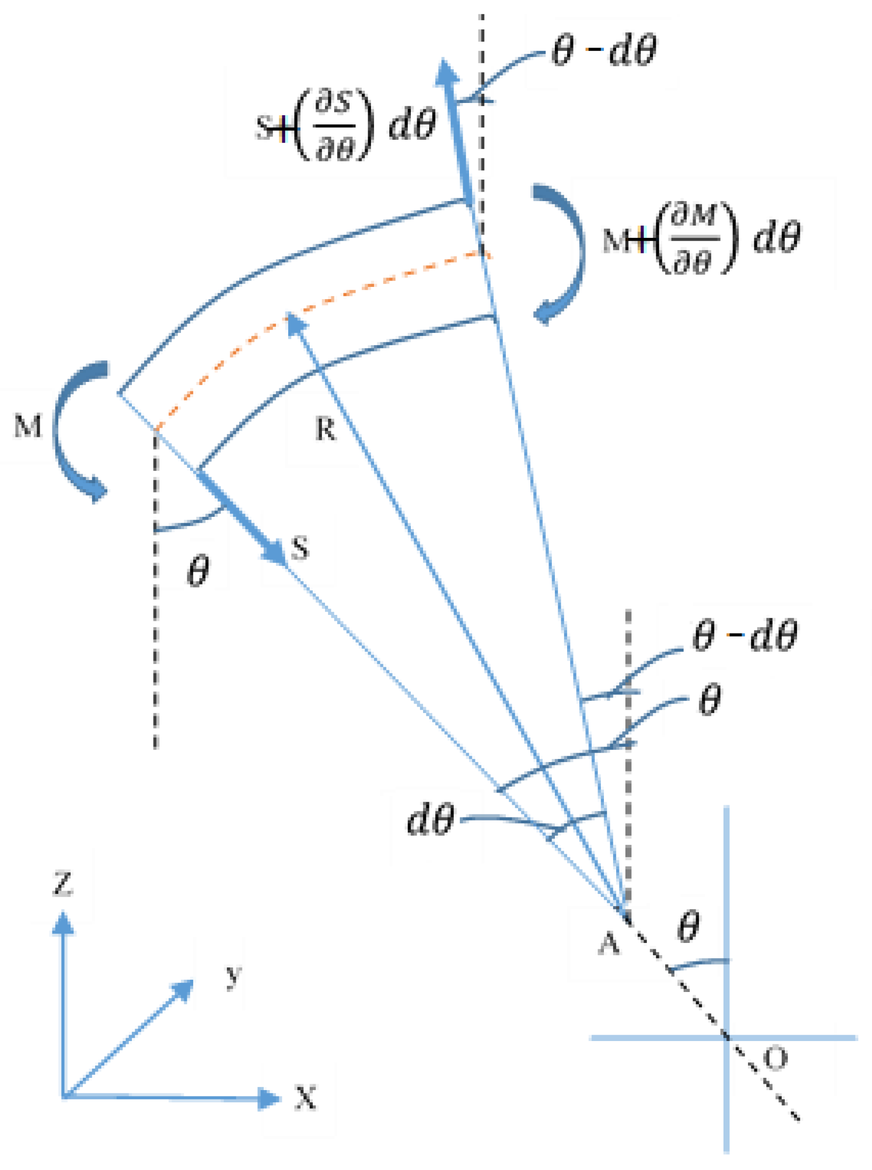
4.1.6. Governing Differential Equations

Let us consider a section of the offshore hose, using the assumptions given in Section 4.1.2. Considering the hose’s motion along the direction that is transverse to mean water level (MWL), the equation of motion is given in Equation (25), as presented in the literature [259], where the hose loading, Q, depends on the hose’s weight, w, alongside the radius of the hose, r, located on the sea, with a water depth h and a hose section bending stiffness of EI_z.

$$E{I}_z\frac{ {\partial }^{4}y}{\partial x^4}+m\frac{ {\partial }^{2}y}{\partial t^2} =Q$$

(25)

A small hose string segment that is relatively short, as given in Figure 11, Figure 12 and Figure 13, can be easily accessed via the governing differential equations [121,122]. In Figure 11, the resultant force, T₀, is localized at point A on the arc length, s. The horizontal force, H₀, is assessed at the CCS locus point, called the origin, O, while V₀ represents the vertical force. Due to the motion of the hose string varying with different durations, different angles will emerge between the axis of the hose string and the horizon, θ_{(i = 1,2,3,..n)}. The times required for a full wave cycle is given by n. The angle between the resultant force’s direction and the horizontal is given by θ₀.

The submarine hose being modeled is considered as a beam under tension, as shown in Figure 12. Normally, two types of differential equations are applied in the analysis of this type of problem. These are the second-order and third-order differential equations; however, a third-order equation is more suitable at the start of the operation. Different approximations have been made from analytical models by some researchers, but these have mostly dealt with floating hoses. The more popular approximations carried out on hoses include the tanh approximation, elastic foundation approximation and buoyancy approximation. The methods applied in the integration of these equations for marine hose’s static analysis include the Runge–Kutta integration method, the fixed mesh difference method and the generalized-α integration method [260,261,262].

Considering the assumptions in Section 4.1.2, the Navier–Stokes equation is applied for an incompressible fluid carrying out a nonrotational motion at sea depth, z, on a floating buoy of depth, d. The velocity potential may be expressed in terms of the fluid quantities, thus yielding:

$$\varphi \left(x,y,t,z\right)=\phi \left(x,y\right)f\left(z\right)e^{i\omega t}$$

(26)

$${\nabla }^2\varphi =0$$

(27)

Considering diffraction theory, there will be no normal flux or normal velocity for impermeable cases, as given in Equation (27); the equation may be simplified and solved by considering the problem in two dimensions (2D), in terms of the velocity potential, denoted as ϕ(x,y), as follows:

$$\nabla \varphi .\stackrel{\rightharpoonup }{n}=\frac{\partial \phi }{\partial n}=0$$

(28)

However, the force on the submarine hose element, F, can be deduced using Cartesian coordinates (x, y, z) or polar coordinates (r, θ, z). As shown in Figure 11, the resultant force is a function of the of the pressure of the fluid_, the sea depth, z and the angle made by the hose element, $\theta$. Similarly, in Figure 13, the total force for the hose segment will be a function of the pressure of the fluid, (P_o and P_i), and the sea depth, z. Thus,

$$\stackrel{\rightharpoonup }{F}\left(\omega \right)=-P\cos \theta dS;-P\sin \theta dS$$

(29)

$$\stackrel{\rightharpoonup }{F}\left(\omega ,t\right)=-{{\displaystyle \int }}_{S}P\stackrel{\rightharpoonup }{r}dS$$

(30)

$$\stackrel{\rightharpoonup }{F}\left(\omega ,t\right)=-{{\displaystyle \int }}_0^{2\pi }{{\displaystyle \int }}_{-d}^{0}P\stackrel{\rightharpoonup }{r}.rd\theta dS$$

(31)

The length of the submarine hose is relative to the sea depth, z and the longitudinal depth profile of the hose, L as seen in Figure 13. A very small section of the submarine hose is considered as the hose element, as represented in Figure 13. The forces acting on it, include the inner pressure denoted as P_i, the outer pressure denoted as P_o, the moment denoted as M, the tension force denoted as T while ds is the small length of the hose element. Also, the supporting floating structure (the CALM buoy) with buoy depth, d is influenced by some dynamic states, which can be discretised. However, for a sea depth z, the force per unit length of the hose element with respect to the depth of the hose from the mean water level (MWL) or surface of the sea is taken to be relative to the existing structure and the global loadings ([263,264,265,266,267]). Thus Equation (31) can be expressed as:

$$\stackrel{\rightharpoonup }{F}\left(z,\omega ,t\right)=-{{\displaystyle \int }}_0^{2\pi }P\stackrel{\rightharpoonup }{r}.rd\theta$$

(32)

4.1.7. Hose Bending and Lateral Deflection

Considering the end at point A as depicted in Figure 14, the distance is x = 0. As the submarine hose strings move due to waves and some vibration motions, an asymptotic relationship can be derived. This is expressed in Equation (33), which gives the movement at the end of the hose string.

$$u\left(x=0\right)=a_h\cos \sigma t$$

(33)

where $a_h$ is the amplitude of the buoy motion, σ is the circular frequency of the wave, ω is the angular frequency, and k is the wave number. It is noteworthy to state that this equation is only accurate when there is steady harmonic motion relative to a straight and lateral configuration of the buoy, positioned backwards. However, for a simpler hose motion in phase, the perturbation from waves can be represented as:

$$u\left(x=0\right)=a_h\left(1-\cos \sigma t\right)$$

(34)

Considering the hose bending and deflection, a displaced beam element is illustrated in Figure 14. It shows the tension forces, bending moments and torsional moments for the displaced hose beam element. This was developed by considering a beam model element undergoing forces and moments with longitudinal displacement u and lateral displacement w, as depicted in Figure 15. The equations of motion in the x-direction and z-direction can be represented as in Equation (35).

In the x-direction, the equation of motion is:

$$S\theta -\left[S+\left(\frac{\partial S}{\partial \theta }\right)d\theta \right]\left(\theta -d\theta \right)=mRd\theta \frac{ {\partial }^{2}u}{\partial t^2}$$

(35)

Diving both sides by dθ and simplifying gives:

$$S-\left(\frac{\partial S\left(\theta +d\theta \right)}{\partial \theta }\right)=mR\frac{ {\partial }^{2}u}{\partial t^2}$$

(36)

Along the z-direction, the equation of motion is:

$$-S+\left[S+\left(\frac{\partial S}{\partial \theta }\right)d\theta \right]=mRd\theta \frac{ {\partial }^{2}w}{\partial t^2}$$

(37)

Diving both sides by dθ and simplifying gives:

$$\left(\frac{\partial S}{\partial \theta }\right)=mR\frac{ {\partial }^{2}u}{\partial t^2}$$

(38)

Taking moments about the edge of the elements in LHS:

$$M-\left[M+\left(\frac{\partial M}{\partial \theta }\right)d\theta \right]+\left[S+\left(\frac{\partial M}{\partial \theta }\right)d\theta \right]Rd\theta =0$$

(39)

Diving both sides by dθ and simplifying gives:

$$-\left[\left(\frac{\partial M}{\partial \theta }\right)\right]+SR+\left[\left(\frac{\partial S}{\partial \theta }\right)d\theta \right]=0$$

(40)

Limiting δS to 0 gives:

$$\frac{\partial M}{\partial \theta }=SR$$

(41)

Applying beam bending theory gives:

$$\frac{M}{EI}=\frac{1}{R}=-\frac{ {\partial }^{2}z}{\partial x^2}$$

(42)

Applying the hose modeling method by O’Donoghue [39,40,41,42], assuming that $\theta =\frac{\partial z}{\partial x}$, $Rd\theta =dx$, and w = z, and incorporating these into Equations (41) and (42), the equation of motion in the longitudinal or x-direction gives rise to Equation (43), and that in the lateral or y-direction gives Equation (44), similar to Equation (25):

$$E{I}_{ }\frac{\partial }{\partial x}\left(\frac{ {\partial }^{3}z}{\partial x^3}.\frac{\partial z}{\partial x}\right)=m\frac{ {\partial }^{2}u}{\partial t^2}$$

(43)

$$E{I}_{ }\frac{ {\partial }^{4}y}{\partial x^4}+m\frac{ {\partial }^{2}y}{\partial t^2} =0$$

(44)

Equation (44) gives the equation of motion for beam bending for the lateral deflection z(x,t) along the length of the beam section [268,269,270], while Equation (43) presents the longitudinal motion of the beam, with the point of force applied at only x = 0, which is the position used in the beam model for the free lateral vibration’s inertial end condition.

4.2. Hydrodynamic Model

In this section, a simple treatise on hydrodynamic forces will be presented, applying the boundary element method (BEM), which is applied when carrying out the hydrodynamics study.

4.2.1. Hydrodynamic Forces

Hydrodynamics affect both the CALM buoy and the attached hoses. When the hose string experiences some hydrodynamic forces, the hose bends. If it is a floating hose, it will bend on the water surface, but if it is a submarine hose, it will bend inside the water body. The damping force is the part of the hydrodynamic force that is proportional to the hose velocity, whereas the added mass force is proportional to the acceleration. The Euler beam approximation of the damping force and added mass force components in the z-axis, can be used to model the dynamical state of the hose beam. The force components for both the damping and the added mass coefficient can be respectively represented as $\left(-Q\frac{\partial z}{\partial t}\right)$ and ($-C_{a}m\frac{ {\partial }^{2}z}{\partial t^2}$), where the damping constant is denoted as Q while the coefficient of added mass is denoted as C_a. By incorporating these terms into Equation (44), we obtain:

$$E{I}_{ }\frac{ {\partial }^{4}y}{\partial x^4}+Q\frac{\partial z}{\partial t}+\left(1+C_a\right) m\frac{ {\partial }^{2}z}{\partial t^2} =0$$

(45)

Similar to the Euler beam approximation, the hydrodynamic damping and added mass force are seen as insignificant in the context of the inertial end condition.

However, O’Donoghue [271,272,273,274] defined C and K via Equations (46) and (47):

$$c^2=\frac{EI}{\left(1+C_a\right)m}$$

(46)

$$K=\frac{Q}{EI}$$

(47)

By applying Equation (33), the equation of motion becomes:

$$\frac{ {\partial }^{4}z}{\partial x^4}+K\frac{\partial z}{\partial t}+\left(\frac{1}{c^2}\right)\frac{ {\partial }^{2}z}{\partial t^2} =0$$

(48)

Considering the inertia end condition gives:

$$[ \frac{\partial }{\partial x}(\frac{ {\partial }^{3}z}{\partial x^3}.\frac{\partial z}{\partial x})]{ }_{x=0} =\frac{a_s}{\left(1+C_a\right)}\left(\frac{{\sigma }^2}{c^2}\right)\cos \left(\sigma t\right)$$

(49)

4.2.2. Snaking Model of Hose

Following the snaking model given in Figure 15, the solution without damping can be considered by taking V = z(x,t) + iy(x,t); assuming that the Euler beam equation without damping is represented by V as K approaches 0 [274] gives

$$\frac{ {\partial }^{4}V}{\partial x^4}+\left(\frac{1}{c^2}\right)\frac{ {\partial }^{2}V}{\partial t^2} =0$$

(50)

and when the inertial end condition is satisfied by z(x,t), this gives Equation (49), thus:

$$[\frac{\partial }{\partial x}(\frac{ {\partial }^{3}z}{\partial x^3}.\frac{\partial z}{\partial x})]{ }_{x=0} =\frac{a_s}{1+C_a}\left(\frac{{\sigma }^2}{c^2}\right)\cos \sigma t$$

(51)

The solution is given in the form $V= A{e}^{-i\omega t}$ when Equation (49) requires values of k = +$k=\pm \frac{\sqrt{\omega }}{c}, \pm \frac{i\sqrt{\omega }}{c}$.

Thus, Equation (49) presents a new solution for the waves in the floating buoy system, where the constants considered are A, B, C and D, expressed as:

$$V= A{e}^{i\left[{\left(\frac{\omega }{c}\right)}^{\frac{1}{2}}x-\omega t\right]}+B{e}^{-i\left[{\left(\frac{\omega }{c}\right)}^{\frac{1}{2}}x-\omega t\right]}+C{e}^{-\left[{\left(\frac{\omega }{c}\right)}^{\frac{1}{2}}x-\omega t\right]e^{-i\omega t}}+D{e}^{\left[{\left(\frac{\omega }{c}\right)}^{\frac{1}{2}}x\right]e^{-i\omega t}}$$

(52)

The terms of B and D tend towards zero in this mathematical formulation based on physical grounds, whereby B = D = 0, as they negate the terms for the waves in A and i, thus:

$$V= A{e}^{i\left[{\left(\frac{\omega }{c}\right)}^{\frac{1}{2}}x-\omega t\right]}+C{e}^{-\left[{\left(\frac{\omega }{c}\right)}^{\frac{1}{2}}x-\omega t\right]e^{-i\omega t}}$$

(53)

where the first term of the RHS of Equation (53) is the traveling wave propagated away by the floating buoy, while the standing wave is represented by the second term, which becomes exponentially lower as x decreases.

By considering the inertial end condition, we obtain:

$$C=0; \omega =\frac{\sigma }{2}; A =2^{\frac{5}{4}}{\left(\frac{a_s}{1+C_a}\right)}^{\frac{1}{2}}{\left(\frac{c}{\sigma }\right)}^{\frac{1}{4}}{e}^{-i\frac{\pi }{4}}$$

(54)

Incorporating Equation (54) into Equation (53) then obtains:

$$V= 2^{\frac{5}{4}}{\left(\frac{a_s}{1+C_a}\right)}^{\frac{1}{2}}{\left(\frac{c}{\sigma }\right)}^{\frac{1}{4}}{e}^{i\left[{\left(\frac{\omega }{c}\right)}^{\frac{1}{2}}x-\omega t\right] \frac{\pi }{4}}$$

(55)

$$V= 2^{\frac{5}{4}}{\left(\frac{a_s}{1+C_a}\right)}^{\frac{1}{2}}{\left(\frac{c}{\sigma }\right)}^{\frac{1}{4}}{e}^{i\left[{\left(\frac{\sigma }{2c}\right)}^{\frac{1}{2}}x-\frac{\sigma }{2}t-\frac{\pi }{4}\right] }$$

(56)

An accurate depiction of the motion of the hose string without damping can be represented as Equation (57), with consideration of the uniqueness of the equation under real conditions. Thus:

$$z\left(x,t\right)= 2^{\frac{5}{4}}{\left(\frac{a_s}{1+C_a}\right)}^{\frac{1}{2}}{\left(\frac{c}{\sigma }\right)}^{\frac{1}{4}}\cos \left[{\left(\frac{\sigma }{2c}\right)}^{\frac{1}{2}}x-\frac{\sigma }{2}t-\frac{\pi }{4}\right]$$

(57)

However, as the hose string’s narrow end approaches x = 0, when x > x₀, then x₀ > 2a_s.

On the other hand, the solution with damping can be considered by taking V = z(x,t) + iy(x,t); by assuming that the Euler beam equation with damping is represented by V as K approaches 0 under inertial end conditions ( [42]), yields:

$$\frac{ {\partial }^{4}V}{\partial x^4}+K\frac{\partial V}{\partial t}+\left(\frac{1}{c^2}\right)\frac{ {\partial }^{2}V}{\partial t^2} =0$$

(58)

Based on the dynamical state of the hose, the form $V= A{e}^{-i\omega t}$ in Equation (58) offers a solution of the form shown in Equation (59), where the constants are depicted as A, B, C and D, while the values of $\alpha ,\beta ,H and \phi$ are given by Bree J. et al. ([274]).

$$V= A{e}^{-\beta x}{e}^{i\left(\alpha x-\omega t\right)}+B{e}^{\beta x}{e}^{i\left(-\alpha x-\omega t\right)}+C{e}^{-\alpha x}{e}^{i\left(-\beta x-\omega t\right)}+D{e}^{\alpha x}{e}^{i\left(\beta x-\omega t\right)}$$

(59)

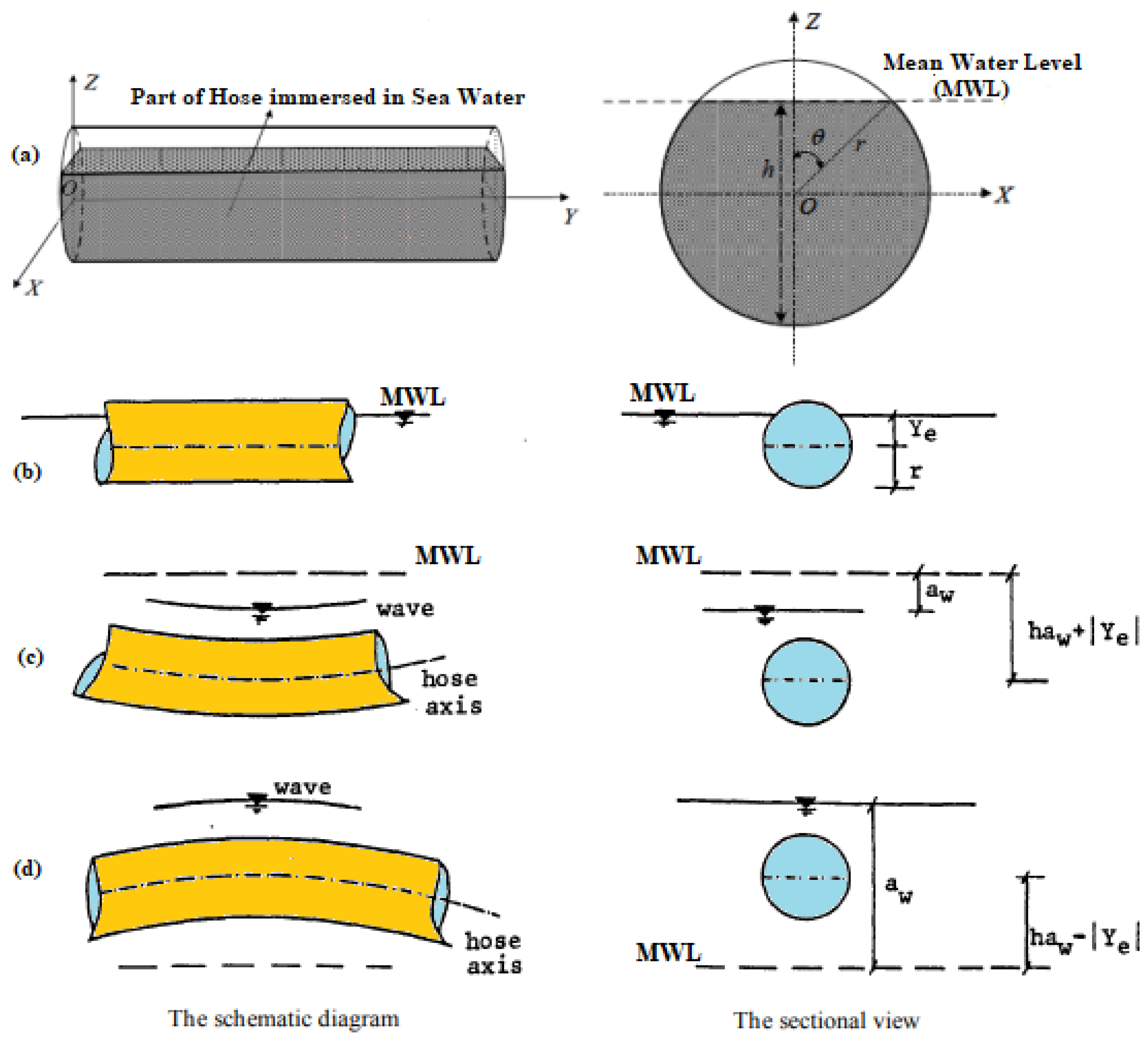
4.2.3. Buoyancy Force

When the marine hose with hose radius r and length S is not submerged in water, it is not acted upon by any buoyancy force because the marine hose is out of the ocean (B_f = 0). This considers the fully submerged hose string depicted in Figure 1, as is the case with submarine hoses, and the force of buoyancy per unit of hose length is denoted by B_f, as shown in Figure 16 for the case of floating hoses. The buoyancy force does not depend on the sea depth when it is completely submerged, thus the buoyancy force is the maximum, B_f(max). However, if it is partially submerged, as is the case with floating hoses, the buoyancy force becomes equal to the weight of the water the hose displaces, and this also depends on the depth below the MWL of the axis of the hose. Thus, the force of buoyancy when the submarine hose is out of water is given by Equation (60), while the buoyancy force for the fully submerged submarine hose is given in Equation (61):

$$B_f=0$$

(60)

$$B_{f\left(max\right)}=\rho gh\left(\pi r^2\right)$$

(61)

4.3. Hose Material Models

The mathematical design of hoses cannot be complete without presenting some hose design models, while discussing material models for the behavior of hoses. Chesterton [6] and Amaechi [19,275] presented a full model of reeling hose in finite element modelling with unique multi-layered scheme, for the hose body and the reinforcement helix, as typified respectively in Figure 17a,b. However, Gao et al. [276] presented a simplified hose model for a 3D hose, with steel helix wire, reinforcement layers and rubber, and addressed symmetry using a 3D quarter model, as shown in Figure 17c.

This helped to save computational time in carrying out the analysis and solving the equations behind the model. However, the later (simple model could not consider reeled sections which the former (full scale model) covered. There are other interesting numerical hose models recently been published on the effect of internal pressure on bonded marine hoses, using methods similar to those of the earlier investigation on multi-layered tubular structures, bonded marine composite hoses and composite risers [277,278,279,280].

In another model by Gonzalez et al. [281], a new approach for modeling the rebars was proposed for marine hoses using polymeric reinforcements. As shown in Figure 18, rebar layers are used to represent polymeric reinforcements embedded in an elastomeric material. Each lamina of fiber reinforcement, referred to as a rebar layer, is suitably positioned within the elastomeric matrix, which is depicted by a continuum finite element similar to the one discussed previously. The relative height of the lamina in relation to the height of the host continuum element totally determines the positioning. This parameter also acts as a constraint between the rebar layer elements and the host element, preventing changes in the relative height value, even after nonlinear analysis deformation. The lay angle, which is given with respect to a chosen global direction, the cross-sectional area of one fiber cable, and the distance between two successive fiber cords are all aspects of the reinforcement that must be defined.

An important feature of hose models is the layers, which are usually made of rubberized or elastomeric materials, while the reinforcements are usually made of steel materials. The end-fitting of the marine hose, as shown in Figure 19, is usually bonded to its layers. As seen in Figure 19a,b, the end fitting has a flange, retention ring or locking ring, nipple, holding plies or textile plies, lining, main plies, helical wires and binding wires or reinforcement wires. The cross-section of the marine hose depicted in Figure 19c shows a hose material with the following layers: the liner, cord-1, bend stiffener, cord-2, cover, cord-3, liner, cord-4, and liner. An important aspect of material assessment is presented in

Table 5. Commonly used elastomers in bonded hoses.

Elastomers	General Attributes
Natural rubber	Excellent physical properties, high elasticity, flexibility, very good abrasion, limited resistance to acids, not resistant to oil
Silicone rubber	Very good hot air resistance approximately up to +250 °C for short periods of time, good low-temperature behavior, ozone and weather resistance, limited oil resistance, not resistant to petrol and acids
NVC (NBR/PVC)	Excellent oil resistance and weather resistance for both lining and cover, not particularly resistant to cold
Fluorinated rubber (Viton)	Excellent high-temperature resistance up to +225 °C and up to +350 °C for short periods of time especially in oil and water, very good chemical resistance
Acrylo-nitrile rubber (Nitrile, NBR)	Excellent oil resistance, limited resistance to aromatic compounds, resistance to fuel and flexibility under cold depend on I content
Chlorosulfonated polyethylene	Excellent weather, ozone, and acid resistance, limited resistance to mineral–oil-derived liquids
Ethylene propylene rubber (EPDM)	Excellent ozone, chemical and ageing properties, low resistance to oil-derived liquids, very good steam resistance, good cold and heat resistance (−40 °C to +175 °C), good resistance to brake fluid based on glycerol
Butyl rubber	Excellent weather resistance, low air and gas permeability, good acid and caustic resistance, good physical properties, good heat and cold resistance, no resistance to mineral–oil-deprived liquids
Chlorinated polyethylene (CPE)	Excellent resistance to ozone and weather, medium resistance to aromatic compounds and oil, excellent flame resistance
Hydrogenated nitrile rubber (HNBR)	Good resistance to mineral–oil-based fluids, animal fats and vegetable fats
Acrylate rubber	Excellent oil and tar resistance at high temperatures
Styrene-butadiene rubber (SBR)	Good physical properties, good abrasion resistance, low resistance to mineral–oil-derived liquids
Chlorobutyl rubber	Variant of butyl rubber
Polychloroprene (Neoprene)	Excellent weather resistance, flame-retardant, medium oil resistance, good physical properties, good abrasion resistance

, regarding the use of a matrix with similar rubber properties for marine hoses, offshore fenders and offshore safety barriers. Rubber models are considered based on different elastomeric attributes when designing, modelling and manufacturing hoses. This is important because different grades of elastomers have different behaviours to certain chemicals, high temperature, corrosive fluids and sea water. Milad et al. [282] and Aboshio et al. [283] analytically investigated the hyperelastic material behavior of a PVC/nitrile elastomer with a woven continuous nylon reinforcement composite sheet based on experimental findings under loading cases of uniaxial extension and pure shear. This was achieved via wide strip tension testing using a novel advanced non-contact optical strain measurement technique, carried out on an Imetrum system, and validated using ABAQUS hyperelastic material models for the curve fittings.

Based on the fiber design, Nooij [202] presented a geodesic model for modeling offloading hoses by applying Integral Geodesic Winding (IGW) technology and Netting theory. In the model, the theory had two limiting assumptions: that the stiffness matrix contribution is negligible and that the wall thickness remains small. This implies that the composite structure will be classified as a thin-walled structure with a thin revolving shell, under external load (A) and internal pressure (Pr), as illustrated in Figure 20. However, when the laminate’s in-plane shear stress equals zero, this design can optimally utilize the maximal strength of its fiber bundle. The study was able to use composites in winding marine hoses, which have better flexibility than helical paths and higher fatigue resistance. However, the trade-off with high pressure (burst load) reported on the IGW hoses [202] was improved by composites in the geodesic design, which helped it to maintain a level position (balance), stable position (stability), and improve resistance to high motion response (vibration).

4.4. Hose Stability Models

Hoses, like submarine pipelines, can be subjected to lateral forces; thus, lateral stability, motion stability, and material stability models exist, as presented in this section.

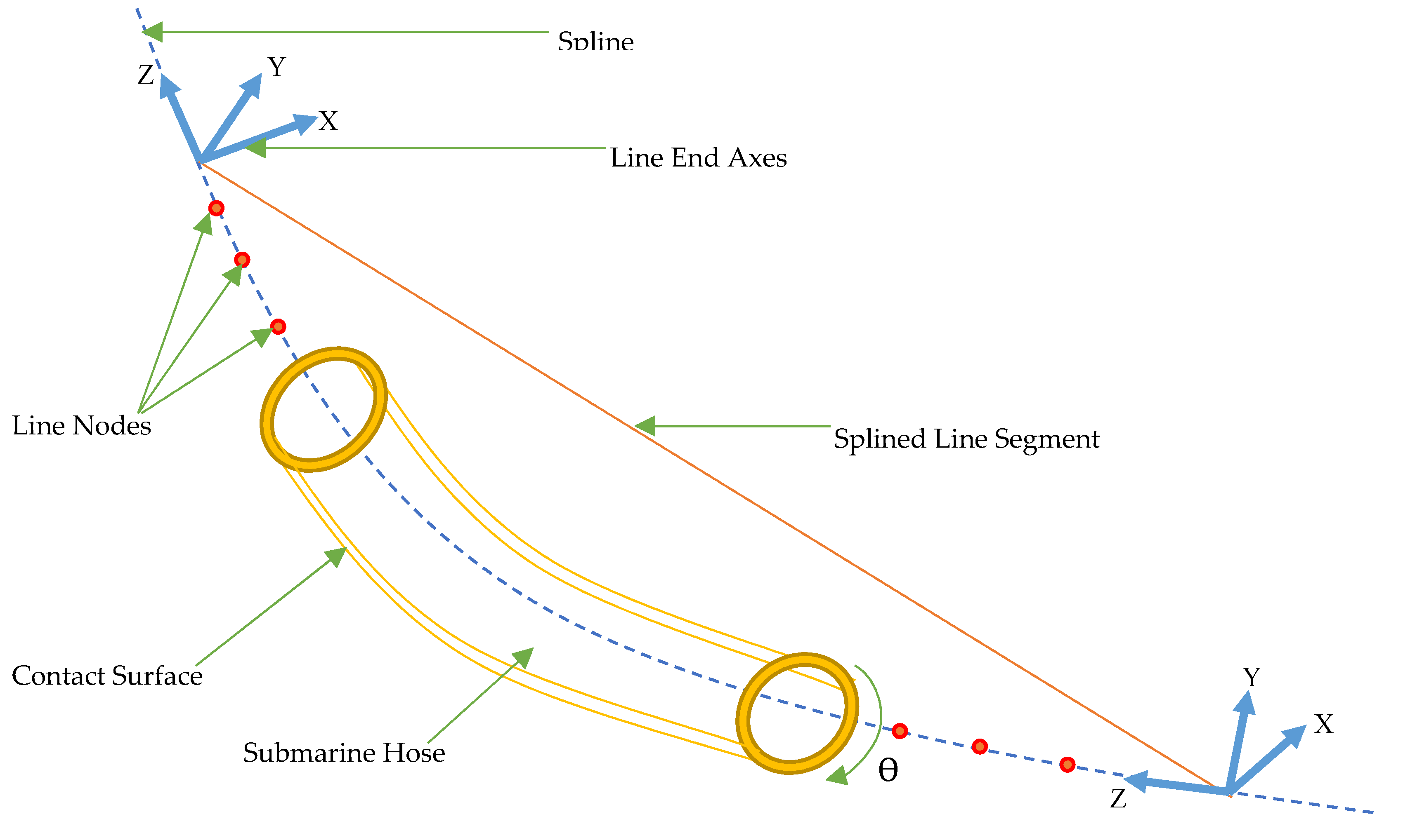
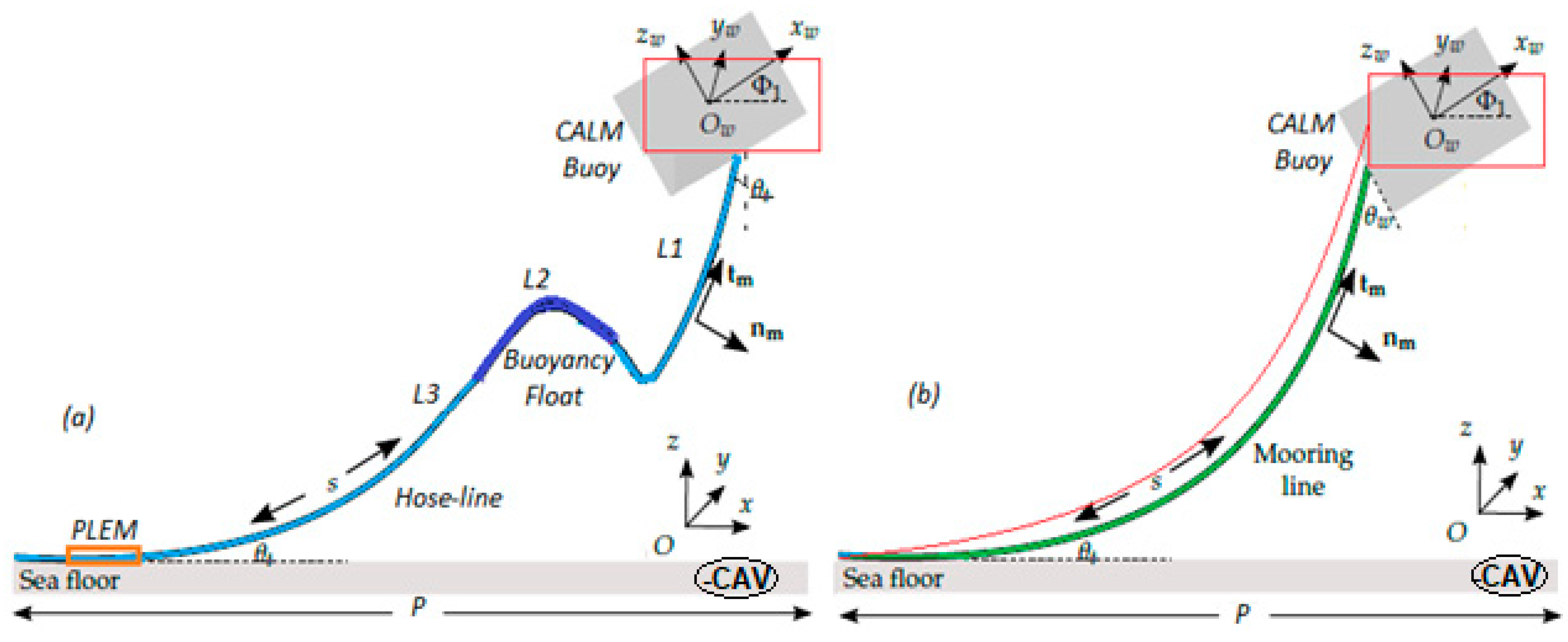
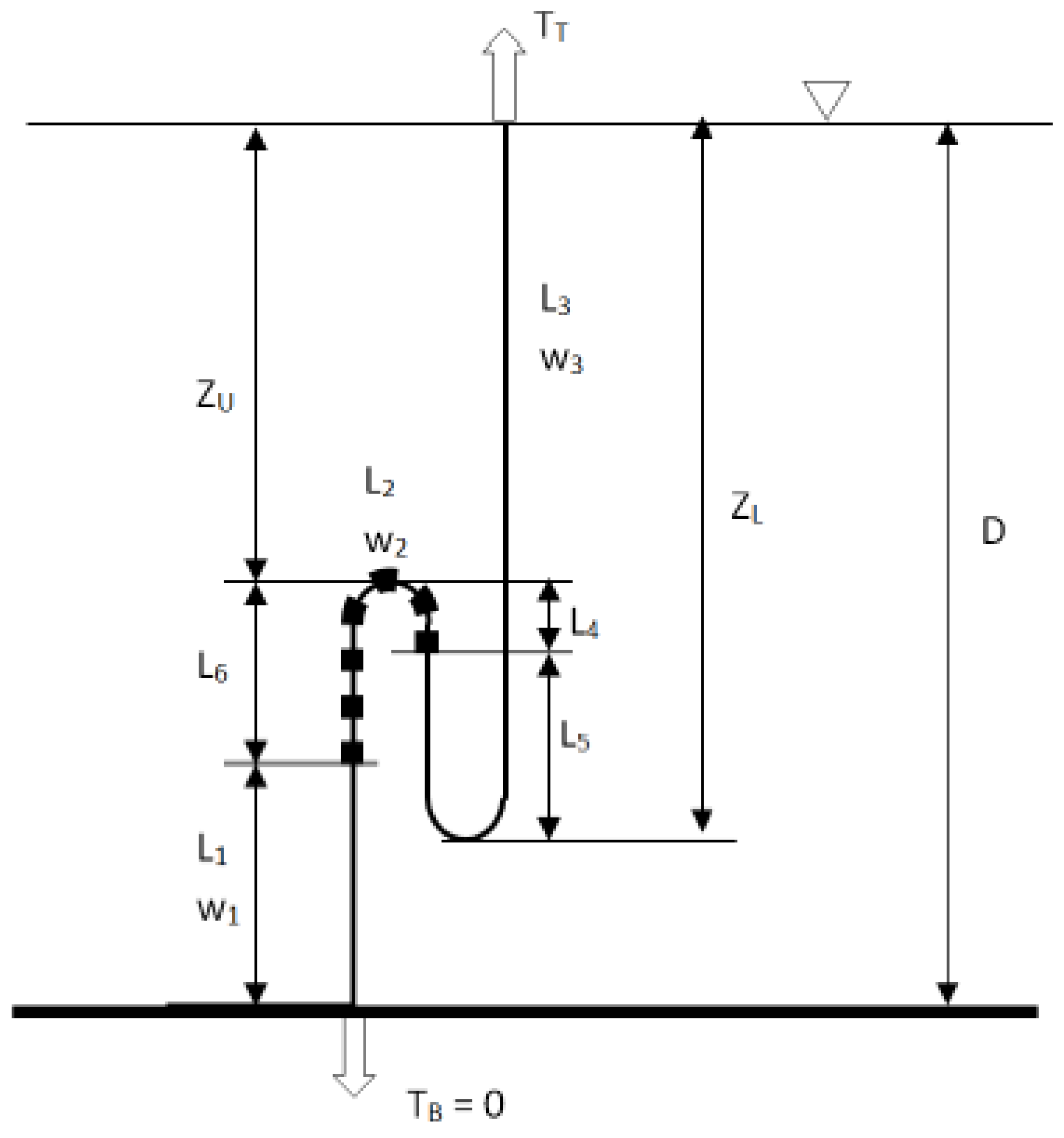
4.4.1. Hose Coordinate Systems

In modeling marine hose systems, three coordinate systems or frames of reference are considered, as illustrated in Figure 21. They are as follows:

(a)

The global frame of reference (x, y, z);

(b)

The CALM buoy frame of reference (x_w, y_w, z_w);

(c)

The curvilinear distance along the hose line, s, also used for moorings.

Both the global and CALM buoy frames of reference are three-dimensional, defining two horizontal and one vertical Cartesian coordinate. The CALM buoy frame of reference’s origin, O_w, is specified at the CALM buoy’s center of mass, while the global frame of reference’s origin, O, can be defined at any appropriate fixed position. The curvilinear distance is a one-dimensional coordinate measured along the hose line (also used for moorings), with s = 0 corresponding to the bottom end linked to the PLEM for hoses and anchors for moorings. Additionally, s = L, corresponding to the top end connected to the CALM buoy (L being the length of the hose line, also used for moorings).

In Figure 21, some angles and vectors are denoted, defined as follows:

Φ is a vector containing three angles—

Φ₁ corresponds to the angle between x and xw due to the CALM buoy pitch displacement;

Φ₂ corresponds to the angle between y and yw due to the CALM buoy roll displacement;

Φ₃ corresponds to the angle between z and zw, due to the CALM buoy yaw displacement.

θ_w is the angle between the mooring line’s top end and the CALM buoy at the connection point;

θ_t is the angle between the mooring line and the ground at the touch-down point on the sea floor;

t_m is the unit vector tangential to the hose line and mooring line;

n_m is the unit vector normal to the hose line and mooring line;

L1, L2 and L3 are section lengths of the hose line.

4.4.2. Environmental Conditions

Waves, currents, wind, and variations in water depth owing to the tide are the environmental inputs that drive the mooring line dynamics, as shown in Figure 1. Due to the action of the waves and currents, external forces are directly imparted onto the mooring lines from the fluid. Furthermore, because to the CALM buoy’s motion, driven by waves, currents and winds, which create some variations in the water depth, a force is applied to the end of the hose line and the mooring line. This also generates some top tension at the hose’s top connection to the buoy manifold. As a result, most hose lines have heavily reinforced ends at the top end to control internal pressure loads, tension forces and wave exciting forces. The exciting forces are a combination of three excitation modes based on environmental inputs, are as follows: Firstly, a mean force, or static loading, is created by the steady current, mean wind, and mean wave drift forces. Secondly, high-frequency (HF) forces are considered for oceans with higher wave characteristics in typical range of 0-0.35Hz, while low-frequency (LF) forces are induced by slowly varying wave drift forces, unsteady wind forces, and slowly varying tidal forces in the general range of 0–0.02 Hz. Thirdly, the wave frequency (WF) forces are induced by first-order wave forces in the general range of 0.03–0.3 Hz. This is applicable in larger floating structures like semisubmersibles. This is also considered in the mathematical computation of the Response Amplitude Operators (RAO) for the motion behaviour of the floating structure.

4.4.3. Hose Slenderness Ratio

In principle, the stability of marine hoses is a function of their slenderness ratio, as they are slender structures. Due to the high span-to-diameter ratio of a marine hose, especially when connected as a hose string, as well as its flexible characteristics, the bending effects are not negligible, unlike flexible riser systems or models [208,284,285].

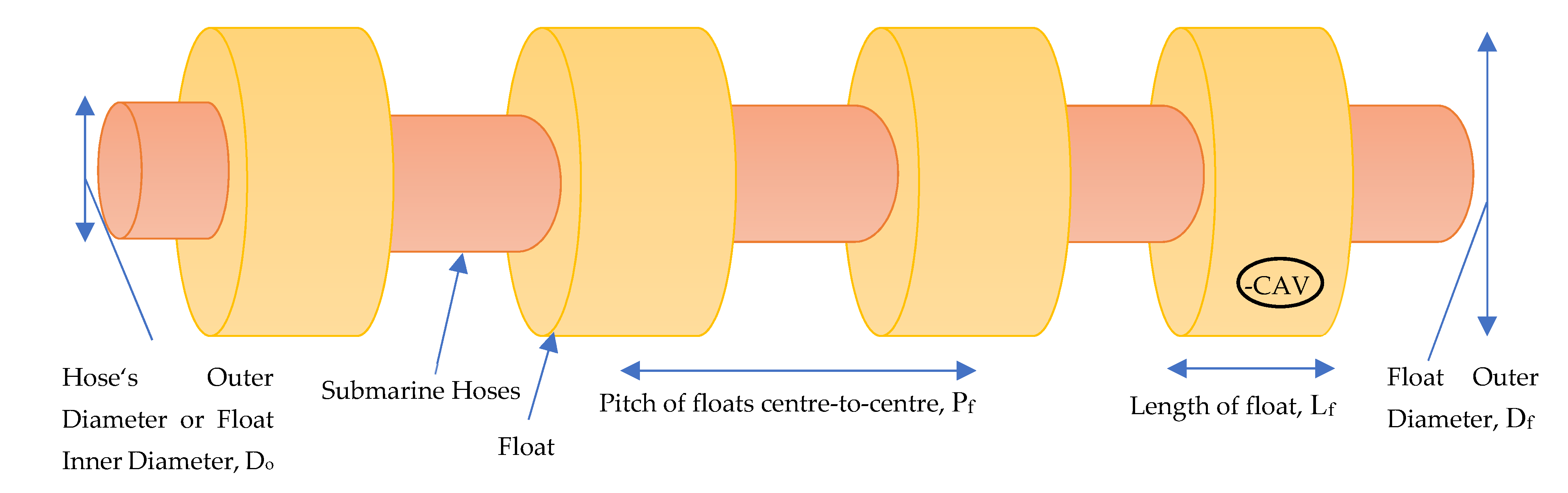
4.5. Hose Floats and Buoyancy Module Models

A buoyancy connection on the hoses was designed with a float incorporated as part of the hose line. The design of float materials is performed in accordance with the industry requirements for OCIMF GMPHOM hoses [3,21,204]. The buoyancy of the submarine hose line is obtained by designing a series of floats arranged together, as depicted in Figure 22. With the application of the equivalence principle of the hydrodynamic loads per unit length and buoyancy load for the buoyancy section, as presented in [286], the equivalent float weight w_e, equivalent float outer diameter D_e, and equivalent hydrodynamic coefficients C_de and C_τe for the buoyancy section can be presented as in Equations (62)–(65), where w is the weight per unit length of riser, ρf is the material density of the buoyancy block, mfh is the mass of attached rigging of the buoyancy float block, and Cτn is the tangential drag coefficient acting on the cross-section of the buoyancy float block. Note that Equation (62) is purely for the case in [286], but not for other hoselines with floats. It defers from other baseline mathematical models for hoselines in Orcaflex documentation [213,214]. However, the equivalent normal and tangential added mass coefficients for the buoyancy section in this case by Ruan et al. [286] can also refer to the equivalent process of drag force coefficients [287], given as:

$$w_e=w+\frac{\pi }{4}\left[{\rho }_f{L}_f\left(D_f^2-D_o^2\right)+m_{fh}\right].\frac{g}{S_f}$$

(62)

$$D_e=\sqrt{\left(D_f{}^2-D_o{}^2\right).\left(\raisebox{1ex}{$L_f$}\!\left/ \!\raisebox{-1ex}{$S_f$}\right.\right)+D_o{}^2)}$$

(63)

$$C_{de}=\frac{C_d}{D_e{S}_f}\left[D_f{L}_f+D_o\left(S_f-L_f\right)\right]$$

(64)

$$C_{\tau e}=\frac{1}{D_e{S}_f}\left[\frac{C_{\tau n}}{4}\left(D_f{}^2-D_o{}^2\right)+C_{dt}{D}_f{L}_f+C_{dt}{D}_o\left(S_f-L_f\right)\right]$$

(65)

5. Governing Equations and Motion Characteristics

In this section, modeling methods and software tools for marine hoses are presented.

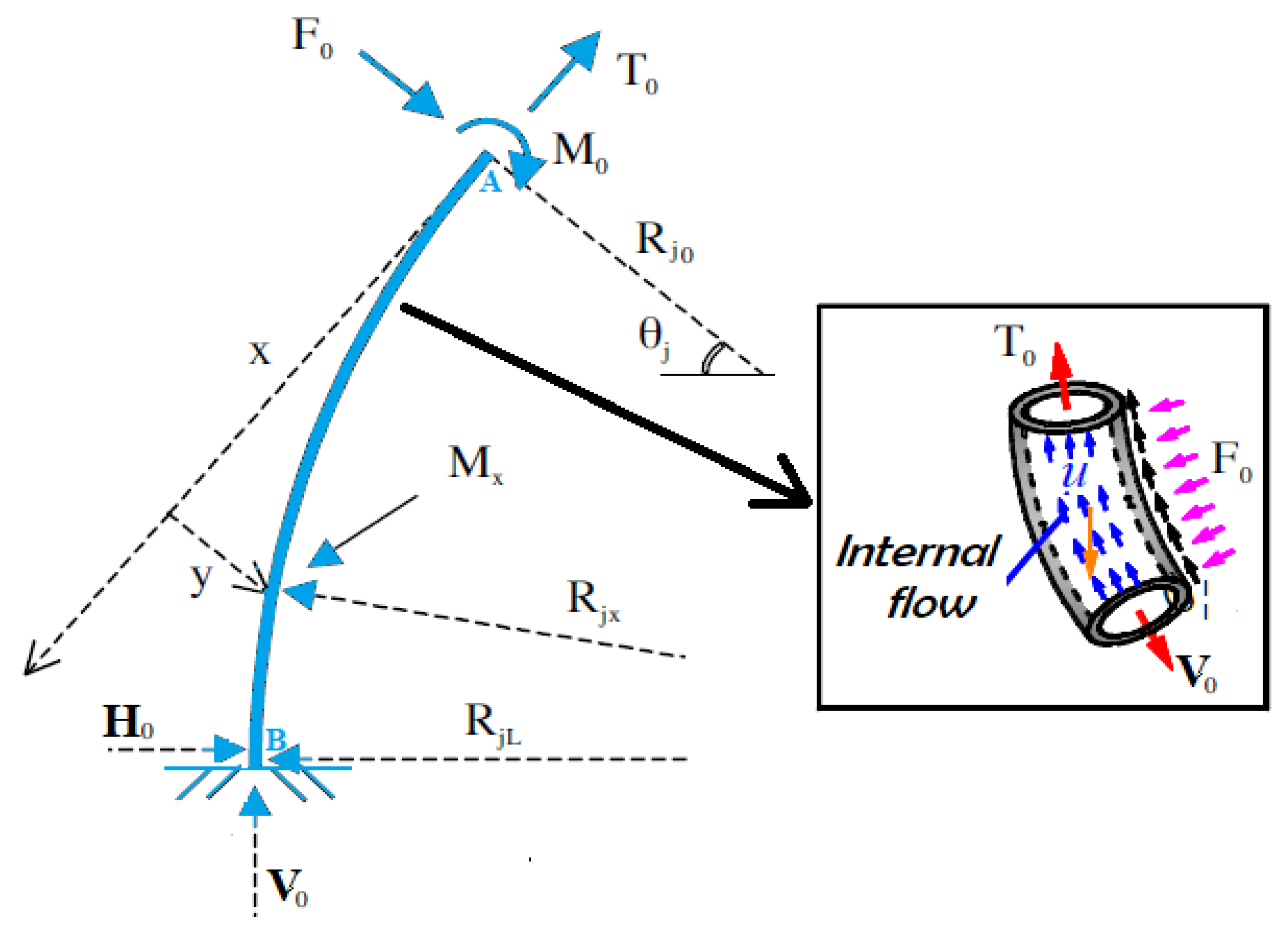
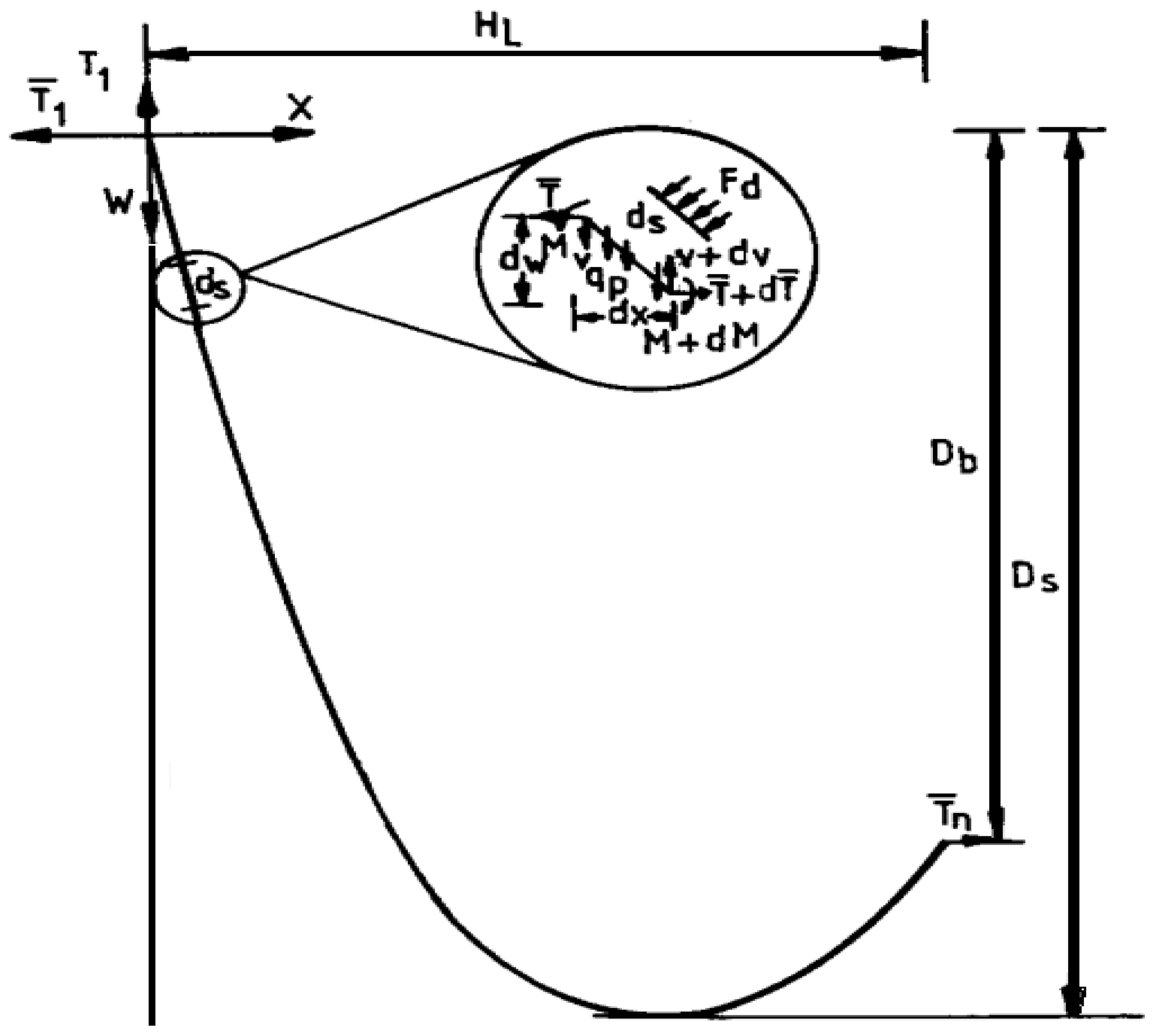
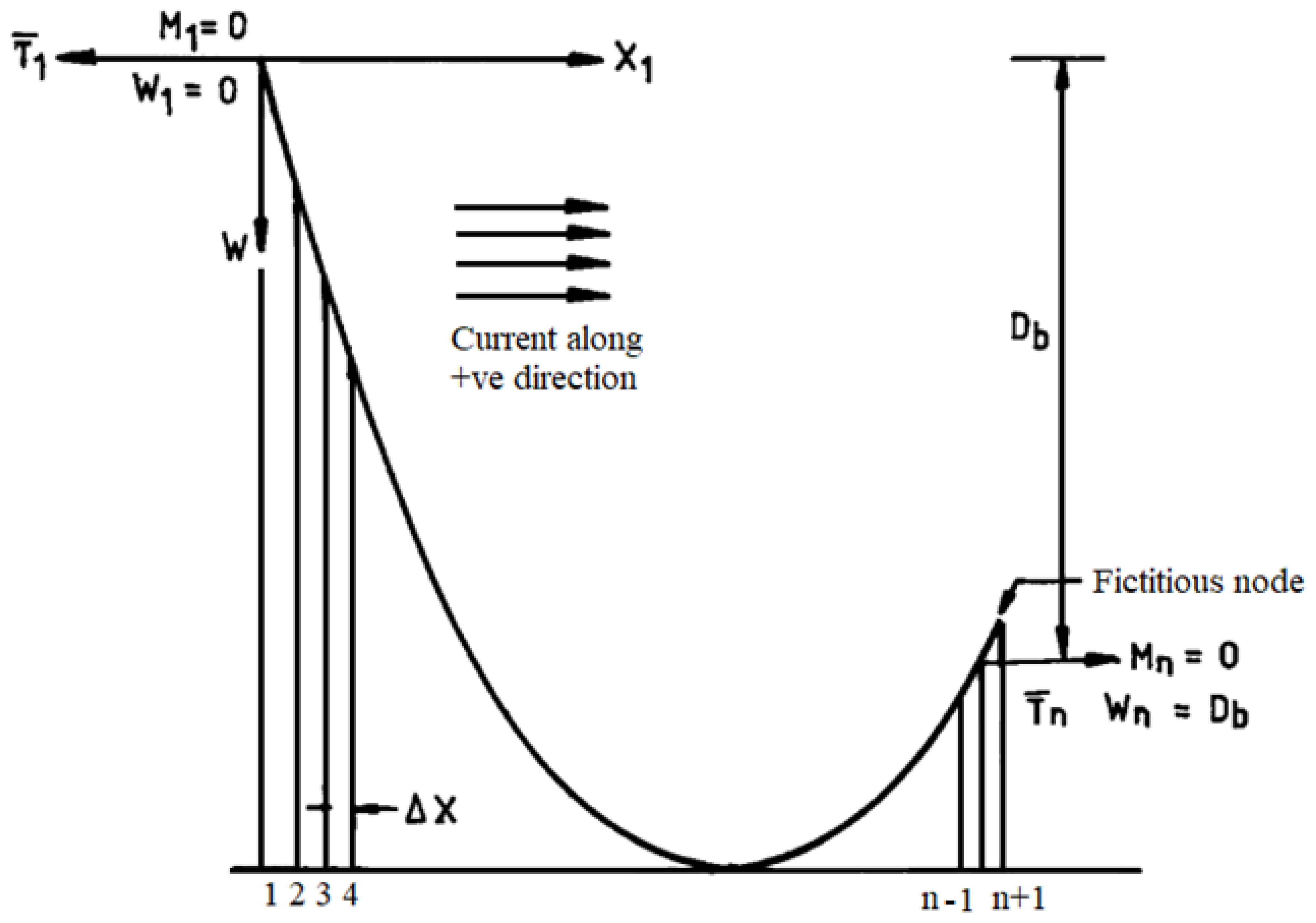
5.1. Static Analysis of Marine Hoses and Risers Subjected to Submerged Self-Weight

The mathematical model of marine hoses that are in a Lazy-S configuration is considered to be similar to that of marine risers under submerged self-weight. To design this, different methods are considered for the elastic line analysis. Of note is the finite difference method as reviewed herein, using earlier considerations for marine hoses on articulated platforms [287,288]. The finite difference method gives a more robust and efficient solution for nonlinear problems that have large angles within the geometrical aspect of the hose’s bending. However, the hose must be designed with limits (2D or 4D, where D is diameter) to its diameter, depending on the type of the hose, as specified in the OCIMF standards [289,290,291].

For marine hoses, most are designed to be buoyant. Marine risers are not designed to include buoyancy, but buoyancy loads are considered among the loads in its design. As such, configurations such as Lazy-S are considerable for marine hoses and marine risers by ensuring that the elastic line has minimal flexural stiffness and hangs between both points of the mid-arch buoy (or floating buoy) and the floater (or FPSO or shuttle vessel). It is this segment that is exposed to most of the environmental loadings, which is considered in the following mathematical modeling.

To develop this, some assumptions have been made for the mathematical model under static and quasi-static loads, as follows:

• The loads acting on the marine hose or marine riser are defined in the analysis;
• The marine hose is considered to be a hose string, similar to a marine riser in a single line;
• The marine hose has its own buoyancy, which is the only buoyancy considered, and it is assumed that there is no additional buoyancy in the system;
• The marine hose exists in a plane that lies in two dimensions, as produced by both static and quasi-static forces;
• Horizontal tension is applied at the hose end attached to the floater (called the floater end), which predominantly controls the marine hose profile;
• It is assumed that the applied horizontal tension is supported by the floater’s anchoring system;
• The two ends of the marine hose are hinged, whereby the end attached to the mid-arch buoy (called the mid-arch buoy end) has negligible moment as a result of the minimal flexural stiffness of the marine hose.

5.2. Motion Behaviour of Marine Hoses and Risers

The equation of motion for marine hoses has been defined in an earlier submarine hose model by Amaechi et al. [50], as given in Equation (66). With particular details regarding the degrees of freedom (DoFs) along the translational direction, the general equation of motion of the body in the horizontal plane can be represented as Equation (66), where {$\ddot{x}$} is the acceleration vector, {$\dot{x}$} is the velocity vector, {x} is the motion vector, [K] is the stiffness matrix, [C] is the damping matrix, [M] is the mass matrix, and {F} is the hydrodynamic exciting force vector of this marine hose system.

$$\left\{F\right\}=\left[M\right]\left\{\ddot{x}\right\}+\left[C\right]\left\{\dot{x}\right\}+\left[K\right]\left\{x\right\}$$

(66)

However, for an articulated hose model, the equation of motion includes the measured movements and the descriptive load effects, as given in Equation (67).

$$m\ddot{x}+c\left[\dot{x}\left(t\right)\right]+k\left[x\left(t\right)\right]=q_a\left(t\right)+q_h\left(t\right)$$

(67)

where the damping forces and restoring forces may theoretically be nonlinear.

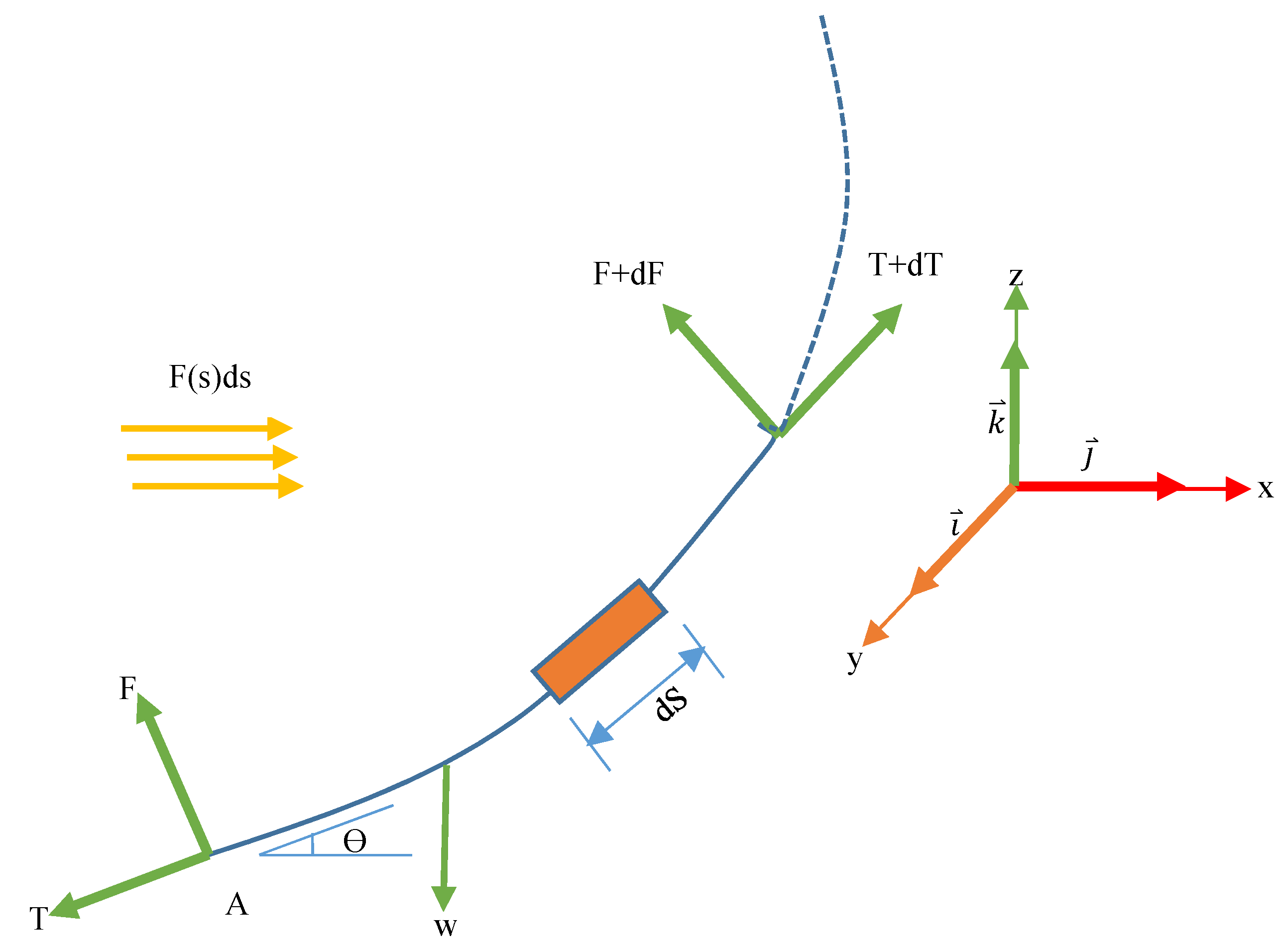
5.3. Static Equilibrium of Marine Hoses and Risers

In addition to the mathematical illustrations shown in Figure 23, some equations from the mathematical model of static equilibrium in marine hoses are presented in this section. The portion of the hose line that is suspended between the hose end and the floater end is depicted in Figure 1. Equation (68) depicts the relationship relating to the static equilibrium of the hose element, with a given length of hose, represented as $\partial s$.

$$\partial V-q_p\partial s-F_d\partial x=0$$

(68)

$$\partial M-V\partial dx-\overline{T}\partial w=0$$

(69)

$$\partial \overline{T}-F_d\partial w=0$$

(70)

where the damping force, $F_d$ can be expressed as:

$$F_d=\rho C_{d}r{V}_c{}^2{\left(\partial w/\partial s\right)}^2$$

(71)

Rewriting Equation (68), we get:

$$V+\overline{T}\frac{\partial w}{\partial x}-\frac{\partial M}{\partial x}=0$$

(72)

Differentiating Equation (72) with respect to x yields

$$\frac{\partial V}{\partial x}+\overline{T}\frac{{\partial }^{2}w}{\partial x^2}+\frac{\partial \overline{T}}{\partial x}.\frac{\partial w}{\partial x}-\frac{{\partial }^{2}M}{\partial x^2}=0$$

(73)

Via the substitution of $\frac{\partial V}{\partial x}$ and $\frac{\partial \overline{T}}{\partial x}$ into Equation (73), using the terms from Equations (67) and (70),

$$\overline{T}\frac{{\partial }^{2}w}{\partial x^2}+F_d{\left(\frac{\partial w}{\partial x}\right)}^2-\frac{{\partial }^{2}M}{\partial x^2}+q_p\frac{\partial s}{\partial x}+F_d=0$$

(74)

For simplicity, it can be convenient to rewrite Equation (74) as:

$$\frac{{\partial }^{2}M}{\partial x^2}-\overline{T}\frac{{\partial }^{2}w}{\partial x^2}+={\overline{q}}_p+{\overline{F}}_d$$

(75)

Equation (75) is a fourth-order differential equation of equilibrium with four boundary conditions in terms of w and x.

In terms of displacement, Jain [288] expressed the equation as:

$$E\overline{I}\frac{{\partial }^{4}M}{\partial x^4}-\overline{T}\frac{{\partial }^{2}w}{\partial x^2}+={\overline{q}}_p+{\overline{F}}_d$$

(76)

where ${\overline{q}}_p$ and ${\overline{F}}_d$ are respectively expressed as:

$${\overline{q}}_p=q_p{\{1+{(\frac{\partial w}{\partial x})}^2\}}^{\frac{1}{2}}$$

(77)

$${\overline{F}}_d=\rho C_{d}r{V}_c{}^2{\left(\partial w/\partial x\right)}^2$$

(78)

For the bending moment, Equation (79) holds:

$$M=E\overline{I}\frac{{\partial }^{2}M}{\partial x^2}$$

(79)

where

$$\overline{I}=\frac{I}{{[1+{(\frac{\partial w}{\partial x})}^2]}^{1.5}}$$

(80)

At a static equilibrium position, the bending moments at the buoy end and the floater end are assumed to equal zero. Thus, the equilibrium relationship in Equation (75) has the following boundary conditions, based on Figure 24.

X = 0 at w = 0; M = 0

(81)

X = H_L at w = D_b, M = 0

(82)

5.4. Equation of Motion of Marine Hoses and Risers

Here, we consider a short hose line assumed to be in a straight line, similar to marine risers, whereby the deformation is relative to its orientation. Bennett and Metcalf [292] presented equations of motion for a structure along a 2D plane, with the equilibrium equations of Equations (83)–(85), constitutive Equations (86) and (87) and kinematic Equations (88)–(90);

$$\frac{\partial P}{\partial x}=-P_x+{\mu }_x\frac{{\delta }^{2}u}{\delta t^2}+k_x\left(x,u\right)u$$

(83)

$$\frac{\partial V}{\partial x}=-P_z+k_z\left(x,w\right)w$$

(84)

$$\frac{\partial M}{\partial x}=-V+\left(P+r\right)\frac{\delta w}{\delta x}-\widehat{t}$$

(85)

where $\widehat{t}$ is applied moment/length, V is transverse shear, u is axial displacement, w is lateral displacement, P is tensional force, x is the axial axis, T is the concentrated applied tension, k is the change in curvature, and r is rotational spring stiffness/length.

As regards the constitutive equations, we have:

$$P=EAϵ$$

(86)

$$M=EI\kappa$$

(87)

$$ϵ=\frac{\delta u}{\delta x}+\frac{1}{2}{(\frac{\delta w}{\delta x})}^2$$

(88)

$$\kappa =\frac{{\delta }^{2}w}{\delta x^2}{[1+\frac{\delta w}{\delta x}]}^2$$

(89)

With the application of rotation theory under conditions of large deflection and moderate conditions of ${(\frac{\delta w}{\delta x})}^2\ll 1$, there are limitation that restrict $(\frac{\delta w}{\delta x})$. Thus, the curvature becomes:

$$\kappa =\frac{{\delta }^{2}w}{\delta x^2}$$

(90)

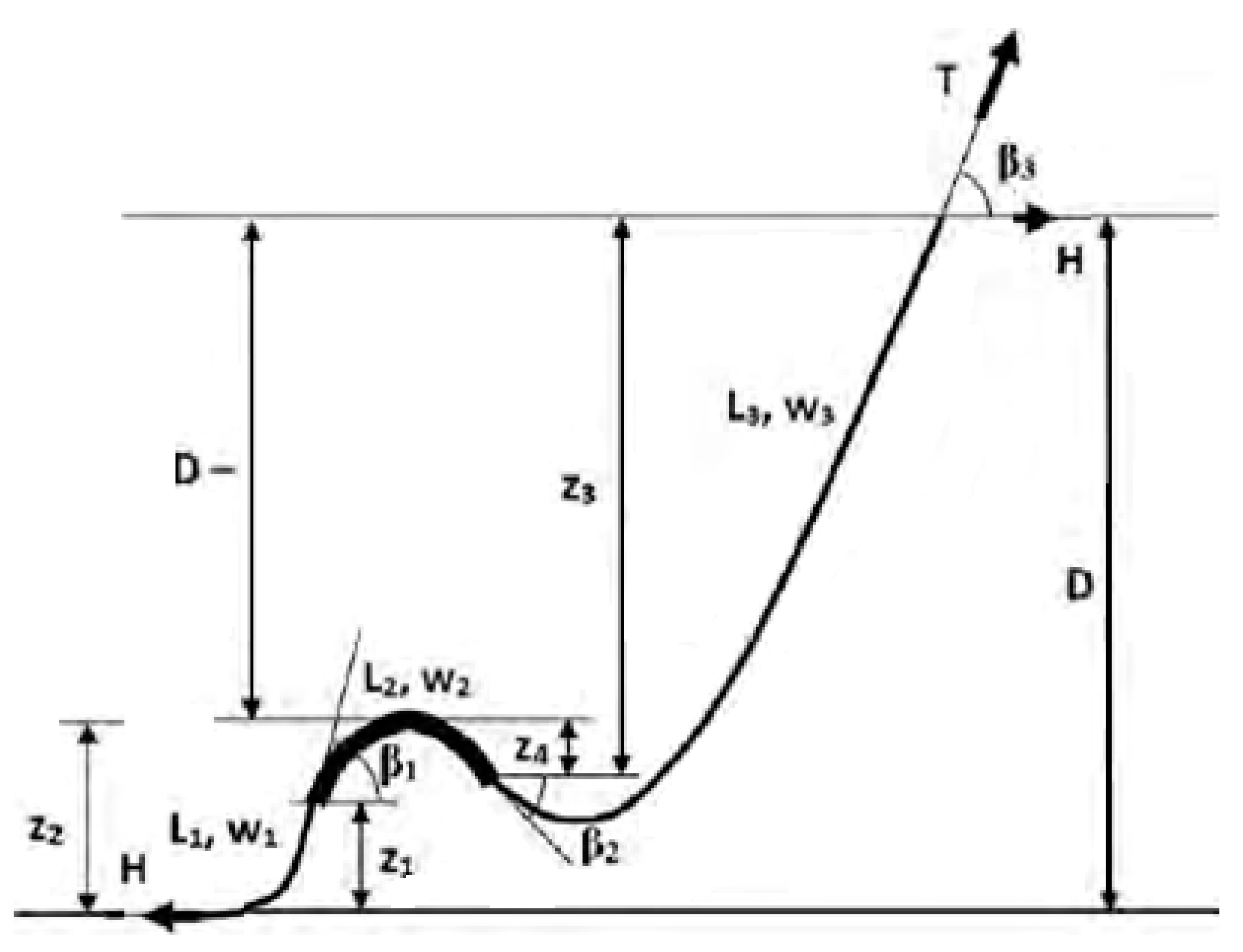
5.5. Analysis of Lazy-Wave Configuration

Permissible bending at the two bends in a “near” position and allowable tension at the upper end in a “far” position are both characteristics of an acceptable design. Vertical equilibrium and compatibility equations can be created, allowing unknown design parameters to be calculated. Three diverse design situations will be addressed with solutions. Initial higher and lower bend positions, as well as the effective weights of segments, are provided; segment lengths can be computed.

5.5.1. First Option

Initial upper and lower bend positions, as well as effective weights of segments, are provided; segment lengths can be computed.

When the desired bend positions and effective weights of all segments are determined, the required segment lengths may be calculated. There are six unknown length parameters in Figure 25, but we also have six equations; four are based on compatibility, and two are based on vertical equilibrium. One assumption here is that the initial condition lies below the MWL. Segment 1 is the lowest segment that partially rests on the bottom. In the initial condition, the length L₁ is vertical and the effective tension T_B equals zero at the touch-down point (TDP). Segment 2 is the segment with uniform buoyancy. Its total length is L₂. This segment will, in the initial condition, have a horizontal tangent at distance Z_u from the upper end (or surface on the figure). This point is referred to as the upper bend. It is noteworthy to state that a horizontal tangent means that tension in the riser must be zero in the initial condition, since the horizontal force equals zero and the hose has no shear force. Segment 3 is the segment that ends at the floater. Segment length is L₃. This segment will in the initial condition have a horizontal tangent at a distance Z_L from upper end. This point is referred to as lower bend. The effective axial force at the upper end will be T_T. For this analysis, w_i is the effective (or submerged) weight per unit length of segment i (N/m), while D is the vertical distance from the upper end to the bottom.

Length of segment 1: L₁ = D − Z_u − L₆

(91)

Length of segment 2: L₂ = L₄ − L₆

(92)

Length of segment 3: L₃ = Z₁ + L₅

(93)

Total length of riser: L₁ + L₂ + L₃ = D + 2(Z_L − Z_u)

(94)

Equilibrium bottom–upper bend: L₆w₂ + L₁w₁ = 0

(95)

Equilibrium of reversed section: L₄w₂ + L₅w₃ = 0

(96)

L₁ = w₂(Z_u − D)/ (w₁ − w₂)

(97)

L₃ = {(D − Z_u − L₁)w₂ + Z_L w₃ − w₂[D + 2(Z_L − Z_u) − L₁]}/(w₃ − w₂)

(98)

L₂ = D + 2(Z_L − Z_u) − L₁ − L₃

(99)

L₄ = L₂ − L₆

(100)

L₅ = L₃ − Z_L

(101)

L₆ = D − Z_u − L₁

(102)

5.5.2. Second Option

The length of the buoyant zone and upper segment, as well as the effective weight of the segments, are specified, and the bend position are computed.

Using some known variables, the unknown parameters include the tension of the upper end, denoted as T_T, the length of the suspended part of segment 1, denoted as L₁, the vertical position of the upper bend, denoted as Z_u, and the vertical position of the lower bend, denoted as Z_L.

In this case, there are three equilibrium equations, and one that defines compatibility:

Equilibrium top–lower bend: T_T = w₃Z_L

(103)

Equilibrium bottom–upper bend: {(D − L₁ − Z_U)w₂ + L₁w₁ } = 0

(104)

Global equilibrium: L₁w₁ + L₂w₂ + L₃w₃ = T_T

(105)

Global compatibility: L₁ + L₂ + L₃ − 2(Z_L − Z_U) = D

(106)

Standard manipulation of these equations gives the following solutions:

Z_L = (2A₁w₁ + A₂w₁w₂ − 2A₃w₁ + A₃w₂)/(2w₁w₃ − w₂w₃ − 2w₁w₂)

(107)

Z_U = (A₂w₁ − A₃ − w₃Z_L + 2Z_Lw₁)/2w₁

(108)

L₁ = (A₃ + w₃Z_L)/w₁

(109)

A₁ = −Dw₂

(110)

A₂ = D − L₂ − L₃

(111)

A₃ = −L₂w₂ − L₃w₃

(112)

5.5.3. Third Option

Upper and lower bend initial positions, effective weight of upper and lower segments, and upper segment length are all specified. The buoyancy segment’s length and effective weight must be computed.

If the desired bend positions are known, vertical equilibrium at the initial position can be used to determine the length and weight of the buoyancy segment. L₁, L₄, L₅, L₆, and w₂ are unknown parameters. The following relationships can be used to find them:

L₅ = L₃ − Z_L

(113)

L₄ = Z_L − Z_u − L₅

(114)

w₂ = −L₅w₃/L₄

(115)

L₁ = {(D − Z_u)w₂}/(w₂ − w₁)

(116)

L₆ = D − Z_u − L₁

(117)

5.6. CALM Catenary Configuration Equations

The governing equation used in the calculation of the statics for the mooring lines is the catenary equation. It is also applied in other applications, such as steel catenary risers (SCR) and cable structures. In the case of mooring lines, which suspend from the CALM buoy to the anchor on the seabed, the catenary shape is approximate, as shown in Figure 26. The catenary line is defined by the following equation (118), where w denotes weight per unit length and H denotes the tension in the horizontal component.

$$y=\frac{H}{w}\left[\cosh \left(w\frac{x}{H}\right)-1\right]$$

(118)

$$T_H=\omega \left[\frac{s^2-h^2}{2.h}\right]$$

(119)

$$T_v=\omega .s$$

(120)

$$T=T_H+h.\omega$$

(121)

The catenary equations for CALM systems are presented in Equations (118)–(124), where h (or z) denotes the height above seabed, s denotes the arc length, x denotes the section length of the mooring cable, w_s denotes the submerged weight, T_H denotes the tension along the horizontal component, T_v denotes the tension along the vertical component, T denotes the tension component along the plane, V denotes the body’s volume and W denotes the body’s weight. The schematic of the catenary mooring system of a CALM buoy is illustrated in Figure 27. The suspended part of the line, s [172] is given by:

$$s=z \sqrt{\left[1+2\left(\frac{T_H}{z\omega }\right)\right]}$$

(122)

$$x=\frac{T_H}{\omega }.\ln [\frac{T}{T_H}+\sqrt{{[\left(\frac{T}{T_H}\right)]}^2-1} ]$$

(123)

$$X=h+X_O-s+x$$

(124)

5.7. Catenary Analysis of Lazy-Wave Configuration

Figure 28 depicts the geometry of a lazy-wave riser as well as all of the required geometry parameters. If the horizontal force H, all weights, and segment lengths are known, and the bottom segment is considered to be long enough to maintain zero vertical force at the bottom end, the unknown parameters are:

L₁ is the lower suspended segment length, and z₂ is the upper bend vertical position.

The riser geometry can be simply determined using classical catenary theory if these parameters can be found. For the two unknown parameters, a direct solution is not available. As a result, an iterative technique must be devised. First, the relationship between L₁ and z₂ must be discovered, and then equations describing compatibility for all segments must be developed.

The link between segments 1 and 2 (bottom and buoyancy segments) is z₂ in the vertical position. The following relationship between z₁ and L₁ is derived from the catenary theory in Equation (125) for a given horizontal force:

$$L_1=\sqrt{z_1{}^2+\frac{2z_{1}H}{w_1}}$$

(125)

Consider segment 1 or the portion of segment 2 between the connection point and the higher bend to find tension in the riser at the connection point between segments 1 and 2. Since we assume there is no shear force in the riser, this is possible. As a result, we have Equation (126):

$$T_1=H+w_1{z}_1=-T_1=-\left[H+w_2\left(z_2-z_1\right)\right]$$

(126)

Since the buoyancy of segment 2 will obviously be greater than its weight, w₂ in Equation (125) is negative. If we assume that z₂ is known, this problem can be solved in Equation (127) with respect to z₁:

$$z_1=\frac{w_2{z}_2 }{w_1-w_2 }$$

(127)

We may find the relationship between L₁ and z₂ without any other unknowns by entering Equation (127) into Equation (125), resulting in Equation (128) and (129):

$$L_1=\sqrt{{[\frac{w_2{z}_2 }{w_1-w_2 }]}^2+\frac{-2[\frac{w_2{z}_2 }{w_1-w_2 }]H}{w_1}}$$

(128)

$$L_1={[{(\frac{w_2{z}_2 }{w_1-w_2 })}^2-\frac{2H{w}_2{z}_2}{w_1\left(w_1-w_2\right)}]}^{0.5}$$

(129)

Compatibility can be determined by combining all of the segments’ vertical projections and comparing the result to the known vertical distance between the upper and lower ends, using the parameters as defined in Figure 28.

Thus, Equations (130) and (131) gives the vertical distances z₃ and z₄:

$$z_3=\frac{H }{w_3 }\sqrt{1+{\beta }_3{}^2}-\frac{H }{w_3 }\sqrt{1+{\beta }_2{}^2}$$

(130)

$$z_4=\frac{H }{w_2 }\sqrt{1+{\beta }_2{}^2}-\frac{H }{w_2 }$$

(131)

When the segment lengths, horizontal force, and riser weights are known, the angles at segment boundaries and higher ends can also be determined, as shown in Equations (132)–(134). Finally, Equation (135) may be used to determine the vertical position of upper bend z₂. See the literature [293] for more information on this calculation.

$${\beta }_1=\frac{w_1{L}_1}{H }$$

(132)

$${\beta }_2={\beta }_1\frac{w_2{L}_2}{H }$$

(133)

$${\beta }_3={\beta }_2\frac{w_3{L}_3}{H }$$

(134)

With the above, the vertical position of the upper bend z₂ can be obtained, using:

$$z_2=D-z_3+z_4$$

(135)

5.8. Fundamental Approaches to the Motion of Marine Hoses and Risers

There are three fundamental approaches that can be used in the mathematical modeling of marine hoses. The dynamic responses of the marine hoses can be modeled as follows:

(a)

Time history analysis by the direct integration approach;

(b)

Time history analysis by the mode superposition approach;

(c)

Frequency domain analysis by the steady-state approach.

Firstly, the direct integration method considers time, and involves step-wise numerical integration. The equations of motion with respect to time have already been defined in earlier sections. They show that the computation can be taken step-by-step, and could be time-consuming. For the second, the mode superposition approach, there is a transposition of the equations of motion into the modal space. The modal shapes are considered in the deformation and buckling of the marine hose, by using the dynamic responses of the marine hose system. This approach is utilised in the FEM of flexible risers [284,285,294,295]. In the third approach, it is assumed that the time-dependent terms are harmonic, with the form shown in Equation (136), with respect to time. With the elimination of time in this equation, the transience of the hose response can be neglected to improve the convergence time of the steady-state solution by making it faster.

$$Y=S{e}^{i\omega t}$$

(136)

where Y is the lateral response of the marine hose, w is the angular frequency and t is the time.

In the consideration of hydrodynamic loads, it is assumed that the current, waves and hose motions occur in the same plane along the beam–column axis, with the same small angle conditions and linear elastic behavior.

5.9. Marine Hose and Riser Response Equations

The hose curvature is given by the inverse of the minimum bending radius (MBR), as:

$$Curvature= \frac{1}{MBR}$$

(137)

The limit of permission for the bending radius is subject to the stiffness, EI, which thus becomes:

$$Minimum Bending Moment, M_o=\frac{EI}{MBR}$$

(138)

Hose bending is a key parameter that requires some sensitive investigation, due to strains in the hose material and other forces on the hose. Figure 29 shows the equivalent force system of marine riser or hose segment for internal fluid and external fluid flows.

When external pressure p_e is also present, a similar approach can be used. Both the lateral pressure effects are removed by adding the force systems acting on the pipe section and the internal fluid, then subtracting the force system operating on the displaced fluid. When external pressure p_e is also present, it is approached in a similar fashion, as depicted in Figure 29 and Figure 30. Conversely, the schematic in Figure 30 presents the force loads and pressures acting along a hose string segments with float collars, for the loads on the (a) floating hose, and (b) submarine hose.

Based on the hose content or marine riser content, the pressure field acting on the internal fluid column is closed and in equilibrium with the weight of the internal fluid. The lateral pressures acting on the pipe wall are equal and opposite to those acting on the internal fluid. Hence, by the superposition and addition of the two force systems, those lateral pressures are eliminated. However, the supposedly axial tension in the fluid column, denoted as −p_iA_i, remains, where p_i is the internal pressure and A_i is the internal cross-sectional area of the pipe [121,122]. This leads to equations for the effective tension T_e and apparent weight w_a of the equivalent system.

The force systems operating on the pipe section and the internal fluid are added together, and then the force systems are subtracted. In Figure 29 and Figure 30, w_t denotes the equivalent system’s weight, w_e denotes the weight of the displaced fluid column, w_a denotes the weight of the internal fluid column, and w_i denotes the weight per unit length of the tube.

The effective tension, $T_e$, denotes the axial tension at any point of the riser calculated by considering only the top tension and the apparent weight of the intervening riser segment [49,50]. The equations of effective tension T_e are expressed as in Equation (139) and (140).

$$T_e=T_{tw}-\left(-p_i{A}_i\right)-\left(-p_i{A}_e\right)$$

(139)

$$T_e=T_{tw}-p_i{A}_i+p_i{A}_e$$

(140)

The apparent weight, w_a, can then be represented by Equation (141):

$$w_a=w_t+w_i-w_e$$

(141)

The resolution of forces along the axial direction of an element of length ds can be represented as:

$$\frac{d{T}_e}{ds}=w_a\cos \phi$$

(142)

Considering the resolution of forces along the vertical plane of an element of length ds with small vertical angles yields:

$$\frac{d{T}_e}{ds} = \frac{d{T}_e}{dx} = w_a$$

(143)

6. Concluding Remarks

A review on the mathematical modeling of bonded marine hoses for single point mooring (SPM) systems, with the application of Catenary Anchor Leg Mooring (CALM) buoys, has been conducted. Due to the need to design, analyses, and optimize bonded marine hoses, mathematical modeling for SPM mooring systems involves many methodologies from other offshore engineering domains. Various modeling strategies of increasing complexity and fidelity are available, with the most realistic models being computationally expensive in comparison to their simpler equivalents. These models are based on wave loads on the offshore structures. The sort of model chosen will be determined by the CALM buoy’s operating principles, the mooring system employed, and the analytic application.

This review has achieved the following:

• A mathematical modeling review of marine hoses, SPM moorings and CALM buoys;
• Assessment of marine hoses used for CALM buoys and single point moorings;
• An overview of single point moorings with the contribution to other marine applications;
• Assessment of marine industry application of mooring models (MMs) and hose models (HMs);
• The mathematical modeling of hose behavior, the effect of waves and hydrodynamics.

Studies reporting on hose mooring array analysis, CALM buoy hose system simulations, extreme loads, CALM buoy hose system control, the use of HMs and MMs in design, hose strength analysis, and hose configuration, are compiled separately in Section 2 and Section 3. As regards mooring, fatigue and heavy load studies suggest the need for the highest quality MMs capable of capturing dynamic tensions and effects across the mooring line. The effect of the mooring system on CALM buoy dynamics, i.e., the mechanical impedance of the mooring system, is essential to CALM buoy modeling and control applications, which generally allow for the use of more basic MMs, but this is rarely detailed in research reports. For the real-time computation of CALM buoy control, as well as long-term simulation, it is beneficial to consider time periods, weather conditions and sea states as case studies by using simpler models in fully developed sea state simulations of HM-MM models of CALM buoy systems. Simple models are used in CALM buoy hose systems, hose mooring array layouts, and the optimization of HM-MM design, with model fidelity increasing as the design and analysis become more advanced. The mathematical model has also been reported as applied in field experiences and safety of marine hoses.

Models of the hydrodynamics of marine hoses are presented in Section 4.2. It is noteworthy that the whole range of phenomena that HMs and MMs can capture covers multiple time scales, including ultra-high-frequency effects such as low-frequency (LF) drift motions, low-frequency (LF) motion variations, wave frequency (WF) oscillations, dynamic tensions, snap loads, load disconnection effects and ultra-low-frequency motion responses. To capture the HF effects, the simulations must use very small time-steps, but large simulation durations are necessary to catch the LF effects. Furthermore, the mooring system and the CALM buoy hose models should be subjected to a variety of sea states and environmental variables, which should be investigated using different simulations. These include utilising FPSOs, floating buoys and the attached marine hoses. To achieve the optimal balance between computational requirements and the accuracy of outcomes, pragmatic decisions about the sort of mathematical models to utilize and which inputs to examine must be made. The review also covers challenges encountered in hose installation, connection and hang-off operations. The state-of-the-art, developments, and recent innovations in mooring applications for SURP (subsea umbilicals, risers and pipelines) have been presented. Finally, this study details the materials required for model implementations in hoses and moorings.

References

1. Trelleborg. Oil & Gas Solutions: Oil & Gas Hoses for Enhanced Fluid Transfer Solutions. In Trelleborg Fluid Handling Solutions. Oil & Marine Hoses: Innovation and Safety for Oil & Gas Transfer Systems; Trelleborg: Clemont-Ferrand, France, 2018; Volume 1, pp. 1–30. [Google Scholar]
2. Bluewater. Buoyed Up: The Future of Tanker Loading/Offloading Operations; Bluewater Energy Services: Amsterdam, The Netherlands, 2009; Available online: https://www.bluewater.com/wp-content/uploads/2013/04/CALM-Buoy-brochure-English.pdf (accessed on 12 July 2021).
3. Yokohama. Seaflex Yokohama Offshore Loading & Discharge Hose; The Yokohama Rubber Co. Ltd: Hiratsuka City, Japan, 2016; Available online: https://www.y-yokohama.com/global/product/mb/pdf/resource/seaflex.pdf (accessed on 17 May 2021).
4. EMSTEC. EMSTEC Loading & Discharge Hoses for Offshore Moorings; EMSTEC: Rosengarten, Germany, 2016; Available online: https://denialink.eu/pdf/emstec.pdf (accessed on 17 September 2021).
5. ARPM. Hose Handbook; IP-2; Association for Rubber Products Manufacturers: Indianapolis, IN, USA, 2019; Available online: https://arpminc.com/publications/category/handbooks-and-guides (accessed on 17 September 2021).
6. Chesterton, C. A Global and Local Analysis of Offshore Composite Material Reeling Pipeline Hose, with FPSO Mounted Reel Drum. Bachelor’s Thesis, Lancaster University, Engineering Department, Bailrigg, UK, 2020. [Google Scholar]
7. Amaechi, C.V. Single Point Mooring (SPM) Hoses and Catenary Anchor Leg Mooring (CALM) Buoys. LinkedIn Pulse. 2021. Available online: https://www.linkedin.com/pulse/single-point-mooring-spm-hoses-catenary-anchor-leg-calm-amaechi (accessed on 1 September 2021).
8. Amaechi, C.V.; Odijie, C.; Sotayo, A.; Wang, F.; Hou, X.; Ye, J. Recycling of Renewable Composite Materials in the Offshore Industry. In Encyclopedia of Renewable and Sustainable Materials; Hashmi, S., Choudhury, I.A., Eds.; Elsevier: Oxford, UK, 2020; Volume 2, pp. 583–613. [Google Scholar] [CrossRef]
9. Amaechi, C.V.; Odijie, C.; Etim, O.; Ye, J. Economic Aspects of Fiber Reinforced Polymer Composite Recycling. In Encyclopedia of Renewable and Sustainable Materials; Hashmi, S., Choudhury, I.A., Eds.; Elsevier: Oxford, UK, 2020; Volume 2, pp. 377–397. [Google Scholar] [CrossRef]
10. Ye, J.; Cai, H.; Liu, L.; Zhai, Z.V.; Amaechi, C.V.; Wang, Y.; Wan, L.; Yang, D.; Chen, X.; Ye, J. Microscale intrinsic properties of hybrid unidirectional/woven composite laminates: Part I: Experimental tests. Compos. Struct. 2021, 262, 113369. [Google Scholar] [CrossRef]
11. Amaechi, C.V. Numerical study on plastic deformation, plastic strains and bending of tubular pipes. Inventions 2021, 9. under review. [Google Scholar]
12. Amaechi, C.V.; Gillet, N.; Odijie, C.A.; Xiaonan, H.; Ye, J. Composite Risers for Deep Waters Using a Numerical Modelling Approach. Compos. Struct. 2019, 210, 486–499. [Google Scholar] [CrossRef] [Green Version]
13. Amaechi, C.V.; Gillett, N.; Odijie, A.C.; Wang, F.; Hou, X.; Ye, J. Local and Global Design of Composite Risers on Truss SPAR Platform in Deep waters, Paper 20005. In Proceedings of the 5th International Conference on Mechanics of Composites, Lisbon, Portugal, 1–4 July 2019; pp. 1–3. [Google Scholar]
14. Amaechi, C.V.; Ye, J. A numerical modeling approach to composite risers for deep waters. In Proceedings of the International Conference on Composite Structures (ICCS20) Proceedings, ICCS20 20th International Conference on Composite Structures, Paris, France, 4–7 September 2017. [Google Scholar]
15. Amaechi, C.V. A review of state-of-the-art and meta-science analysis on composite risers for deep seas. Ocean. Eng. 2021. under review. [Google Scholar]
16. Amaechi, C.V. Development of composite risers for offshore applications with review on design and mechanics. Ships Offshore Struct. 2021. under review. [Google Scholar]
17. Amaechi, C.V. Local tailored design of deep water composite risers subjected to burst, collapse and tension loads. Ocean Eng. 2021. under review. [Google Scholar]
18. Gillett, N. Design and Development of a Novel Deepwater Composite Riser. Bachelor’s Thesis, Lancaster University, Engineering Department, Lancaster, UK, 2018. [Google Scholar]
19. Amaechi, C.V. Novel Design, Hydrodynamics and Mechanics of Composite Risers in Oil/Gas Applications: Case Study with Marine Hoses. Ph.D. Thesis, Lancaster University, Engineering Department, Lancaster, UK, 2021. [Google Scholar]
20. Esmailzadeh, E.; Goodarzi, A. Stability analysis of a CALM floating offshore structure. Int. J. Non-Linear Mech. 2001, 36, 917–926. [Google Scholar] [CrossRef]
21. Sun, L.; Zhang, X.; Kang, Y.; Chai, S. Motion response analysis of FPSO’s CALM buoy offloading system. Paper Number OMAE2015-41725. In Proceedings of the International Conference on Ocean, Offshore and Arctic Engineering, St. John’s, NW, Canada, 31 May–5 June 2015; pp. 1–7. [Google Scholar] [CrossRef]
22. Qi, X.; Chen, Y.; Yuan, Q.; Xu, G.; Huang, K. Calm Buoy and Fluid Transfer System Study. In Proceedings of the 27th International Ocean and Polar Engineering Conference, San Francisco, CA, USA, 25–30 June 2017; Available online: https://onepetro.org/ISOPEIOPEC/proceedings-abstract/ISOPE17/All-ISOPE17/ISOPE-I-17-128/17225 (accessed on 12 July 2021).
23. Duggal, A.; Ryu, S. The dynamics of deepwater offloading buoys. In WIT Transactions on The Built Environment. Fluid Structure Interaction and Moving Boundary Problem; WIT Press: Southampton, UK, 2005; Available online: https://www.witpress.com/Secure/elibrary/papers/FSI05/FSI05026FU.pdf (accessed on 17 May 2021).
24. Le Cunff, C.; Ryu, S.; Duggal, A.; Ricbourg, C.; Heurtier, J.; Heyl, C.; Liu, Y.; Beauclair, O. Derivation of CALM Buoy coupled motion RAOs in Frequency Domain and Experimental Validation. In Proceedings of the International Society of Offshore and Polar Engineering Conference, Lisbon, Portugal, 1–6 July 2007; pp. 1–8. Available online: https://www.sofec.com/wp-content/uploads/white_papers/2007-ISOPE-Derivation-of-CALM-Buoy-Coupled-Motion-RAOs-in-Frequency-Domain.pdf (accessed on 19 July 2021).
25. Le Cunff, C.; Ryu, S.; Heurtier, J.-M.; Duggal, A.S. Frequency-Domain Calculations of Moored Vessel Motion Including Low Frequency Effect. In Proceedings of the ASME 2008 27th International Conference on Offshore Mechanics and Arctic Engineering, Estoril, Portugal, 15–20 June 2008; pp. 689–696. [Google Scholar] [CrossRef] [Green Version]
26. Salem, A.G.; Ryu, S.; Duggal, A.S.; Datla, R.V. Linearization of Quadratic Drag to Estimate CALM Buoy Pitch Motion in Frequency-Domain and Experimental Validation. J. Offshore Mech. Arct. Eng. 2012, 134, 011305. [Google Scholar] [CrossRef]
27. D Rutkowski, G. A Comparison Between Conventional Buoy Mooring CBM, Single Point Mooring SPM and Single Anchor Loading SAL Systems Considering the Hydro-meteorological Condition Limits for Safe Ship’s Operation Offshore. TransNav Int. J. Mar. Navig. Saf. Sea Transp. 2019, 13, 187–195. [Google Scholar] [CrossRef] [Green Version]
28. Huang, Z.J.; Santala, M.J.; Wang, H.; Yung, T.W.; Kan, W.; Sandstrom, R.E. Component Approach for Confident Predictions of Deepwater CALM Buoy Coupled Motions: Part 1—Philosophy. In Proceedings of the ASME 2005 24th International Conference on Offshore Mechanics and Arctic Engineering, Halkidiki, Greece, 12–17 June 2005; pp. 349–356. [Google Scholar] [CrossRef]
29. Santala, M.J.; Huang, Z.J.; Wang, H.; Yung, T.W.; Kan, W.; Sandstrom, R.E. Component Approach for Confident Predications of Deepwater CALM Buoy Coupled Motions: Part 2—Analytical Implementation. In Proceedings of the ASME 2005 24th International Conference on Offshore Mechanics and Arctic Engineering, Halkidiki, Greece, 12–17 June 2005; pp. 367–375. [Google Scholar] [CrossRef]
30. Kang, Y.; Sun, L.; Kang, Z.; Chai, S. Coupled Analysis of FPSO and CALM Buoy Offloading System in West Africa. Paper Number: OMAE2014-23118. In Proceedings of the ASME 2014 33rd International Conference on Ocean, Offshore and Arctic Engineering, San Francisco, CA, USA, 8–13 June 2014. [Google Scholar] [CrossRef]
31. Ryu, S.; Duggal, A.S.; Heyl, C.N.; Liu, Y. Prediction of Deepwater Oil Offloading Buoy Response and Experimental Validation. Int. J. Offshore Polar Eng. 2006, 16, 1–7. [Google Scholar]
32. O’Sullivan, M. Predicting interactive effects of CALM buoys with deepwater offloading systems. Offshore Mag. 2003, 63, 66–68. [Google Scholar]
33. O’Sullivan, M. West of Africa CALM Buoy Offloading Systems. MCS Kenny Offshore Technical Note for Flexcom-3D Version 5.5.2, MCS International. 2002. Available online: http://www.mcskenny.com/downloads/Software-OffshoreArticle.pdf (accessed on 17 May 2018).
34. Roveri, F.E.; Volnei, S.; Sagrilo, L.; Cicilia, F.B. A Case Study on the Evaluation of Floating Hose Forces in a C.A.L.M. System. In Proceedings of the International Offshore and Polar Engineering Conference, Kitakyushu, Japan, 26–31 May 2002; Volume 3, pp. 190–197. Available online: https://onepetro.org/ISOPEIOPEC/proceedings-abstract/ISOPE02/All-ISOPE02/ISOPE-I-02-030/8329 (accessed on 15 August 2021).
35. Wang, D.; Sun, S. Study of the Radiation Problem for a CALM Buoy with Skirt. Shipbuild. China 2015, 56, 95–101. [Google Scholar]
36. Pecher, A.; Foglia, A.; Kofoed, J.P. Comparison and sensitivity investigations of a CALM and SALM type mooring system for wave energy converters. J. Mar. Sci. Eng. 2014, 2, 93–122. [Google Scholar] [CrossRef]
37. Hasanvand, E.; Edalat, P. A Comparison of the Dynamic Response of a Product Transfer System in CALM and SALM Oil Terminals in Operational and Non-Operational Modes in the Persian Gulf region. Int. J. Coast. Offshore Eng. 2021, 5, 1–14. [Google Scholar]
38. Hasanvand, E.; Edalat, P. Comparison of Dynamic Response of Chinese Lantern and Lazy-S Riser Configurations Used in CALM Oil Terminal. Mar.-Eng. 2021, 17, 37–52. [Google Scholar]
39. Hasanvand, E.; Edalat, P. Sensitivity Analysis of the Dynamic Response of CALM Oil Terminal, in The Persian Gulf Region Under Different Operation Parameters. J. Mar. Eng. 2020, 16, 73–84. [Google Scholar]
40. Bidgoli, S.I.; Shahriari, S.; Edalat, P. Sensitive Analysis of Different Types of Deep Water Risers to Conventional Mooring Systems. Int. J. Coast. Offshore Eng. 2017, 5, 45–55. [Google Scholar]
41. Berhault, C.; Guerin, P.; le Buhan, P.; Heurtier, J.M. Investigations on Hydrodynamic and Mechanical Coupling Effects for Deepwater Offloading Buoy. In Proceedings of the International Offshore and Polar Engineering Conference, Toulon, France, 23–28 May 2004; Volume 1, pp. 374–379. [Google Scholar]
42. Doyle, S.; Aggidis, G.A. Development of multi-oscillating water columns as wave energy converters. Renew. Sustain. Energy Rev. 2019, 107, 75–86. [Google Scholar] [CrossRef] [Green Version]
43. Zhang, D.; George, A.; Wang, Y.; Gu, X.; Li, W.; Chen, Y. Wave tank experiments on the power capture of a multi-axis wave energy converter. J. Mar. Sci. Technol. 2015, 20, 520–529. [Google Scholar] [CrossRef]
44. Zhang, D.; Shi, J.; Si, Y.; Li, T. Multi-grating triboelectric nanogenerator for harvesting low-frequency ocean wave energy. Nano Energy 2019, 61, 132–140. [Google Scholar] [CrossRef]
45. Amaechi, C.V.; Chesterton, C.; Butler, H.O.; Wang, F.; Ye, J. Review on the design and mechanics of bonded marine hoses for Catenary Anchor Leg Mooring (CALM) buoys. Ocean Eng. 2021, in press. [Google Scholar]
46. Amaechi, C.V.; Chesterton, C.; Butler, H.O.; Wang, F.; Ye, J. An overview on Bonded Marine Hoses for sustainable fluid transfer and (un)loading operations via Floating Offshore Structures (FOS). J. Mar. Sci. Eng. 2021, 9. under review. [Google Scholar]
47. Amaechi, C.V. Development of bonded marine hoses for sustainable loading and discharging operations in the offshore-renewable industry. J. Pet. Sci. Eng. 2021. under review. [Google Scholar]
48. Amaechi, C.V.; Ye, J. Offshore applications of Composite marine risers and submarine hoses in deep waters. In Composite Marine Risers and Submarine Hose Applications for Deep Waters; 20 Minutes Talk; Engineering Department, Lancaster University: Lancaster, UK, 2018; Available online: https://www.research.lancs.ac.uk/portal/en/publications/offshore-applications-ofcomposite-marine-risers-and-submarine-hoses-in-deep-waters(08f8a84b-8e1b-41dc-962e-9203f2aaa62c).html (accessed on 17 May 2021).
49. Amaechi, C.V.; Ye, J.; Hou, X.; Wang, F.-C. Sensitivity Studies on Offshore Submarine Hoses on CALM Buoy with Comparisons for Chinese-Lantern and Lazy-S Configuration OMAE2019-96755. In Proceedings of the 38th International Conference on Ocean, Offshore and Arctic Engineering, Glasgow, Scotland, 9–14 June 2019. [Google Scholar]
50. Amaechi, C.V.; Wang, F.; Hou, X.; Ye, J. Strength of submarine hoses in Chinese-lantern configuration from hydrodynamic loads on CALM buoy. Ocean Eng. 2019, 171, 429–442. [Google Scholar] [CrossRef] [Green Version]
51. Young, R.A.; Brogren, E.E.; Chakrabarti, S.K. Behavior of Loading Hose Models in Laboratory Waves and Currents. In Offshore Technology Conference Proceeding; OTC-3842-MS; OnePetro/OTC: Houston, TX, USA, 1980; pp. 421–428. [Google Scholar] [CrossRef]
52. Zou, J. Vim Response of a Dry Tree Paired-Column Semisubmersibles Platform and Its Effects on Mooring Fatigue. In Proceedings of the SNAME 19th Offshore Symposium, Houston, TX, USA, 6 February 2014; Available online: https://onepetro.org/SNAMETOS/proceedings-abstract/TOS14/1-TOS14/D013S006R002/3701 (accessed on 17 May 2021).
53. Das, S.; Zou, J. Characteristic Responses of a Dry-Tree Paired-Column and Deep Draft Semisubmersible in Central Gulf of Mexico. In Proceedings of the 20th Offshore Symposium, Texas Section of the Society of Naval Architects and Marine Engineers, Houston, TX, USA, 17 February 2015; Available online: https://onepetro.org/SNAMETOS/proceedings-abstract/TOS15/1-TOS15/D013S004R003/3695 (accessed on 17 May 2021).
54. Bhosale, D. Mooring Analysis of Paired-Column Semisubmersible. Bachelor’s Thesis, Lancaster University, Engineering Department, Lancaster, UK, 2017. [Google Scholar]
55. Zou, J.; Poll, P.; Antony, A.; Das, S.; Padmanabhan, R.; Vinayan, V.; Parambath, A. VIM Model Testing and VIM Induced Mooring Fatigue of a Dry Tree Paired-Column Semisubmersible Platform. In Proceedings of the Offshore Technology Conference, Houston, TX, USA, 5–8 May 2014. [Google Scholar] [CrossRef] [Green Version]
56. Amaechi, C.V.; Wang, F.; Ye, J. Numerical investigation on mooring line configurations of a Paired Column Semisubmersible for its global performance in deep water condition. Ocean Eng. 2021. under review. [Google Scholar]
57. Amaechi, C.V.; Wang, F.; Ye, J. Dynamic analysis of tensioner model applied on global response with marine riser recoil and disconnect. Ocean Eng. 2021. under review. [Google Scholar]
58. Amaechi, C.V.; Wang, F.; Ye, J. Parametric investigation on tensioner stroke analysis, recoil analysis and disconnect for the marine drilling riser of a Paired Column Semisubmersible under deep water waves. Ocean Eng. 2021. under review. [Google Scholar]
59. Amaechi, C.V. Effect of marine riser integration for characteristic motion response studies on a Paired Column Semisubmersible in deep waters. Mar. Struct. 2021. under review. [Google Scholar]
60. Odijie, A.C. Design of Paired Column Semisubmersible Hull. Ph.D. Thesis, Lancaster University, Engineering Department, Lancaster, UK, 2016. Available online: https://eprints.lancs.ac.uk/id/eprint/86961/1/2016AgbomeriePhD.pdf (accessed on 12 February 2020).
61. Odijie, A.C.; Wang, F.; Ye, J. A review of floating semisubmersible hull systems: Column stabilized unit. Ocean Eng. 2017, 144, 191–202. [Google Scholar] [CrossRef] [Green Version]
62. Odijie, A.C.; Quayle, S.; Ye, J. Wave induced stress profile on a paired column semisubmersible hull formation for column reinforcement. Eng. Struct. 2017, 143, 77–90. [Google Scholar] [CrossRef] [Green Version]
63. Odijie, A.C.; Ye, J. Effect of Vortex Induced Vibration on a Paired-Column Semisubmersible Platform. Int. J. Struct. Stab. Dyn. 2015, 15, 1540019. [Google Scholar] [CrossRef]
64. Odijie, A.C. Understanding Fluid-Structure Interaction for high amplitude wave loadings on a deep-draft paired column semi-submersible platform: A finite element approach. In Proceedings of the International Conference on Light Weight Design of Marine Structures, Glasgow, UK, 9–11 November 2015. [Google Scholar]
65. Friis-Madsen, E.; Sørensen, H.; Parmeggiani, S. The development of a 1.5 MW Wave Dragon North Sea Demonstrator. In Proceedings of the 4th International Conference on Ocean Energy (ICOE 2012), Dublin, Ireland, 17–19 October 2012; pp. 1–5. Available online: https://www.icoe-conference.com/publication/the_development_of_a_1.5_mw_wave_dragon_north_sea_demonstrator/ (accessed on 17 May 2021).
66. Davidson, J.; Ringwood, J.V. Mathematical Modelling of Mooring Systems for Wave Energy Converters—A Review. Energies 2017, 10, 666. [Google Scholar] [CrossRef] [Green Version]
67. Penalba, M.; Giorgi, G.; Ringwood, J.V. Mathematical modelling of wave energy converters: A review of nonlinear approaches. Renew. Sustain. Energy Rev. 2017, 78, 1188–1207. [Google Scholar] [CrossRef] [Green Version]
68. Giorgi, G.; Penalba, M.; Ringwood, J. Nonlinear Hydrodynamic Models for Heaving Buoy Wave Energy Converters. In Proceedings of the Asian Wave and Tidal Energy Conference, Singapore, 25–27 October 2016; Available online: http://mural.maynoothuniversity.ie/9418/1/JR-Nonlinear-2016.pdf (accessed on 4 March 2021).
69. Kalogirou, A.; Bokhove, O. Mathematical and numerical modelling of wave impact on wave-energy buoys. In Proceedings of the International Conference on Ocean, Offshore and Arctic Engineering, Busan, Korea, 19–24 June 2016; pp. 1–8. [Google Scholar] [CrossRef] [Green Version]
70. Huang, T.S.; Leonard, J.W. Lateral Stability of a Flexible Submarine Hoseline; US Military, Port Hueneme: Oxnard, CA, USA, 1989; Available online: https://apps.dtic.mil/sti/pdfs/ADA219251.pdf (accessed on 8 September 2021).
71. Obokata, J. On the basic design of single point mooring (1st Report)-Applications of the Dynamic Stability Analysis to the Primary Planning of the System. J. Soc. Nav. Archit. Jpn. 1987, 161, 183–195. [Google Scholar] [CrossRef] [Green Version]
72. Obokata, J.; Nakajima, T. On the basic design of single point mooring system (2nd report)-Estimation of the Mooring Force. J. Soc. Nav. Archit. Jpn. 1988, 163, 252–260. [Google Scholar] [CrossRef] [Green Version]
73. Sao, K.; Numata, T.; Kikuno, S. Basic Equation and SALM Buoy Motion. J. Soc. Nav. Archit. Jpn. 1987, 1987, 257–266. [Google Scholar] [CrossRef] [Green Version]
74. Lenci, S.; Callegari, M. Simple analytical models for the J-lay problem. Acta Mech. 2005, 178, 23–39. [Google Scholar] [CrossRef]
75. Luongo, A.; Zulli, D. Mathematical Models of Beams and Cables; John Wiley & Sons, Inc: London, UK, 2013. [Google Scholar] [CrossRef]
76. Irvine, H.M. Cable Structures; MIT Press: Cambridge, MA, USA, 1981; pp. 1–259. [Google Scholar]
77. Berteaux, H.O.; Goldsmith, R.A.; Schott, W.E., III. Heave and Roll Response of Free Floating Bodies of Cylindrical Shape; Report WHOI-77-12; Woods Hole Oceanographic Institution: Falmouth, MA, USA, 1977; Available online: https://apps.dtic.mil/sti/pdfs/ADA038215.pdf (accessed on 15 August 2021).
78. Berteaux, H.O. Buoy Engineering; John Wiley and Sons: New York, NY, USA, 1976. [Google Scholar]
79. Newman, J.N. The Motions of a Spar Buoy in Regular Waves; Report No. 1499; Massachusetts Institute of Technology, Hydromechanics Laboratory: Cambridge, MA, USA, 1963; Available online: http://hdl.handle.net/1721.3/48955 (accessed on 25 July 2021).
80. Ibinabo, I.; Tamunodukobipi, D.T. Determination of the Response Amplitude Operator(s) of an FPSO. Engineering 2019, 11, 541–556. [Google Scholar] [CrossRef] [Green Version]
81. Baghfalaki, M.; Das, S.K.; Das, S.N. Analytical model to determine response amplitude operator of a floating body for coupled roll and yaw motions and frequency based analysis. Int. J. Appl. Mech. 2012, 4, 1–20. [Google Scholar] [CrossRef]
82. Das, S.K.; Baghfalaki, M. Mathematical modelling of response amplitude operator for roll motion of a floating body: Analysis in frequency domain with numerical validation. J. Marine. Sci. Appl. 2014, 13, 143–157. [Google Scholar] [CrossRef]
83. Katayama, T.; Hashimoto, K.; Asou, H.; Komori, S. Development of a Motion Stabilizer for a Shallow-Sea-Area Spar Buoy in Wind, Tidal Current and Waves. J. Ocean Wind. Energy 2015, 2, 182–192. [Google Scholar] [CrossRef]
84. Bao, J.; Wu, Q.; Xie, J.; Jiang, N.; Ma, L.; Zhang, Z.; Dai, H.; Chen, H.; Liu, L. Design and analysis of a wave-piercing buoy. In Automotive, Mechanical and Electrical Engineering; CRC Press: London, UK, 2017; pp. 69–73. [Google Scholar]
85. Jiang, D.; Zhang, J.; Ma, L.; Chen, H.; Qiu, Y.; Li, B.; Liu, L. Effect of heave plate on wave piercing buoy. In Automotive, Mechanical and Electrical Engineering; CRC Press: Boca Raton, FL, USA, 2017; pp. 367–370. [Google Scholar] [CrossRef]
86. Jiang, D.; Li, W.; Chen, X.; Chen, H. The strength analysis of the wave piercing buoy. AIP Conf. Proc. 2017, 1834, 030030. [Google Scholar] [CrossRef] [Green Version]
87. Graber, H.C.; Terray, E.A.; Donelan, M.A.; Drennan, W.M.; Van Leer, J.C.; Peters, D.B. ASIS—A New Air–Sea Interaction Spar Buoy: Design and Performance at Sea. J. Atmos. Ocean. Technol. 2000, 17, 708–720. [Google Scholar] [CrossRef]
88. Zhu, X.; Yoo, W.-S. Numerical modeling of a spherical buoy moored by a cable in three dimensions. Chin. J. Mech. Eng. 2016, 29, 588–597. [Google Scholar] [CrossRef]
89. Beirão, P.J.B.F.N.; Malça, C.M.D.S.P. Design and analysis of buoy geometries for a wave energy converter. Int. J. Energy Environ. Eng. 2014, 5, 1–11. [Google Scholar] [CrossRef] [Green Version]
90. Kim, J.; Kweon, H.-M.; Jeong, W.-M.; Cho, I.-H.; Cho, H.-Y. Design of the dual-buoy wave energy converter based on actual wave data of East Sea. Int. J. Nav. Arch. Ocean Eng. 2015, 7, 739–749. [Google Scholar] [CrossRef] [Green Version]
91. Zhu, X.; Yoo, W.S. Dynamic analysis of a floating spherical buoy fastened by mooring cables. Ocean Eng. 2016, 121, 462–471. [Google Scholar] [CrossRef]
92. Stearns, T.B. Computer Simulation of Underbuoy Hoses. Master’s Thesis, California State University, Northridge, CA, USA, 1975. Available online: https://scholarworks.calstate.edu/downloads/qj72p950b?locale=en (accessed on 17 May 2021).
93. Sweeney, T.E. The Concept of an Unmanned Transatlantic Sailing Buoy (NOAA’s Ark), AMS Report No. 1358; DTIC_ADA132160; Princeton University, Department of Aerospace and Mechanical Sciences: Princeton, NJ, USA, 1977; Available online: https://ia600100.us.archive.org/19/items/DTIC_ADA132160/DTIC_ADA132160.pdf (accessed on 17 May 2021).
94. Wang, Y.-L. Design of a cylindrical buoy for a wave energy converter. Ocean Eng. 2015, 108, 350–355. [Google Scholar] [CrossRef]
95. Wang, F.; Chen, J.; Gao, S.; Tang, K.; Meng, X. Development and sea trial of real-time offshore pipeline installation monitoring system. Ocean Eng. 2017, 146, 468–476. [Google Scholar] [CrossRef]
96. Vickers, A.; Johanning, L. Comparison of damping properties for three different mooring. In Proceedings of the 8th European Wave and Tidal Energy Conference, Uppsala, Sweden, 7–10 September 2009. [Google Scholar]
97. Bergdahl, L.; Palm, J.; Eskilsson, C.; Lindahl, J. Dynamically Scaled Model Experiment of a Mooring Cable. J. Mar. Sci. Eng. 2016, 4, 5. [Google Scholar] [CrossRef] [Green Version]
98. Cozijn, J.L.; Bunnik, T.H.J. Coupled Mooring Analysis for a Deep Water CALM Buoy. In Proceedings of the ASME 2004 23rd International Conference on Offshore Mechanics and Arctic Engineering, Vancouver, BC, Canada, 20–25 June 2004; pp. 663–673. [Google Scholar] [CrossRef] [Green Version]
99. Cozijn, H.; Uittenbogaard, R.; Brake, E.T. Heave, Roll and Pitch Damping of a Deepwater CALM Buoy with a Skirt. In Proceedings of the Fifteenth International Offshore and Polar Engineering Conference, Seoul, Korea, 19–24 June 2005; pp. 388–395. Available online: https://onepetro.org/ISOPEIOPEC/proceedings-abstract/ISOPE05/All-ISOPE05/ISOPE-I-05-296/9432# (accessed on 15 August 2021).
100. Williams, N.A.; McDougal, W.G. Experimental Validation of a New Shallow Water CALM Buoy Design. In Proceedings of the ASME 2013 32nd International Conference on Ocean, Offshore and Arctic Engineering, Nantes, France, 9–14 June 2013; pp. 1–6. [Google Scholar] [CrossRef]
101. Capobianco, R.; Rey, V.; Le Calvé, O. Experimental survey of the hydrodynamic performance of a small spar buoy. Appl. Ocean Res. 2002, 24, 309–320. [Google Scholar] [CrossRef]
102. Ricbourg, C.; Berhault, C.; Camhi, A.; Lecuyer, B.; Marcer, R. Numerical and Experimental Investigations on Deepwater CALM Buoys Hydrodynamics Loads. In Proceedings of the Offshore Technology Conference, Houston, TX, USA, 1–4 May 2006; pp. 1–8. [Google Scholar]
103. Eriksson, M.; Isberg, J.; Leijon, M. Theory and Experiment on an Elastically Moored Cylindrical Buoy. IEEE J. Ocean. Eng. 2006, 31, 959–963. [Google Scholar] [CrossRef]
104. Saito, H.; Mochizuki, T.; Fukai, T.; Okui, K. Actual measurement of external forces on marine hoses for SPM. In Proceedings of the Offshore Technology Conference Proceeding-OTC 3803, Houston, TX, USA, 19–20 March 1980; pp. 89–97. [Google Scholar]
105. Edward, C.; Dev, A.K. Assessment of CALM Buoys Motion Response and Dominant OPB/IPB Inducing Parameters on Fatigue Failure of Offshore Mooring Chains. In Practical Design of Ships and Other Floating Structures. PRADS 2019. Lecture Notes in Civil Engineering; Okada, T., Suzuki, K., Kawamura, Y., Eds.; Springer: Singapore, 2021; Volume 64. [Google Scholar]
106. Jean, P.; Goessens, K.; L’Hostis, D. Failure of Chains by Bending on Deepwater Mooring Systems. In Proceedings of the Paper presented at the Offshore Technology Conference, Houston, TX, USA, 2–5 May 2005. [Google Scholar] [CrossRef]
107. Denney, D. Chain Failure by Bending on Deepwater Mooring Systems. J. Pet. Technol. 2006, 58, 72–73. [Google Scholar] [CrossRef]
108. HSE. Floating Production System—JIP FPS Mooring Integrity. Prepared by Noble Denton Europe Limited for the Health and Safety Executive. Research Report 444. HSE Books: Crown, UK, 2006. Available online: https://www.hse.gov.uk/research/rrpdf/rr444.pdf (accessed on 17 May 2021).
109. Brown, M.G.; Hall, T.D.; Marr, D.G.; English, M.; Snell, R.O. Floating Production Mooring Integrity JIP—Key Findings. In Proceedings of the Offshore Technology Conference Held, Houston, TX, USA, 2–5 May 2005. [Google Scholar] [CrossRef]
110. Amaechi, C.V.; Wang, F.; Ye, J. Numerical studies on CALM buoy motion responses, and the effect of buoy geometry cum skirt dimensions with its hydrodynamic waves-current interactions. Ocean Eng. 2021. under review. [Google Scholar]
111. Amaechi, C.V.; Wang, F.; Ye, J. Numerical Assessment on the Dynamic Behaviour of Submarine Hoses Attached to CALM Buoy Configured as Lazy-S Under Water Waves. J. Mar. Sci. Eng. 2021, 9, 1130. [Google Scholar] [CrossRef]
112. Amaechi, C.V.; Wang, F.; Ye, J. Understanding the fluid-structure interaction from wave diffraction forces on CALM buoys: Numerical and analytical solutions. Ships Offshore Struct. J. 2021. under review. [Google Scholar]
113. Amaechi, C.V. Investigation on hydrodynamic characteristics, wave-current interaction and sensitivity analysis of submarine hoses attached to a CALM buoy. J. Mar. Sci. Eng. 2021, 9. under review. [Google Scholar]
114. Amaechi, C.V. Experimental, analytical and numerical study on CALM buoy hydrodynamic motion response and the hose-snaking phenomenon of the attached marine hoses under water waves. J. Mar. Sci. Eng. 2021. under review. [Google Scholar]
115. Tonatto, M.L.; Tita, V.; Amico, S.C. Composite spirals and rings under flexural loading: Experimental and numerical analysis. J. Compos. Mater. 2020, 54, 2697–2705. [Google Scholar] [CrossRef]
116. Tonatto, M.L.P.; Tita, V.; Forte, M.M.C.; Amico, S.C. Multi-scale analyses of a floating marine hose with hybrid polyaramid/polyamide reinforcement cords. Mar. Struct. 2018, 60, 279–292. [Google Scholar] [CrossRef]
117. Tonatto, M.L.P.; Roese, P.B.; Tita, V.; Forte, M.M.C.; Amico, S.C. Offloading marine hoses: Computational and experimental analyses. In Marine Composites: Design and Performance, 1st ed.; Summerscales, J., Graham-Jones, J., Pemberton, R., Eds.; Woodhead Publishing: New York, NY, USA, 2018; Volume 1, pp. 389–416. [Google Scholar]
118. Tonatto, M.L.P.; Forte, M.M.; Tita, V.; Amico, S. Progressive damage modeling of spiral and ring composite structures for offloading hoses. Mater. Des. 2016, 108, 374–382. [Google Scholar] [CrossRef]
119. Tonatto, M.L.P.; Tita, V.; Araujo, R.T.; Forte, M.M.; Amico, S. Parametric analysis of an offloading hose under internal pressure via computational modeling. Mar. Struct. 2017, 51, 174–187. [Google Scholar] [CrossRef]
120. Szczotka, M. Dynamic analysis of an offshore pipe laying operation using the reel method. Acta Mech. Sin. 2011, 27, 44–55. [Google Scholar] [CrossRef]
121. Sparks, C.P. Fundamental of Marine Riser Mechanics: Basic Principles and Simplified Analysis, 2nd ed.; PennWell Corporation Books: Tulsa, OK, USA, 2018. [Google Scholar]
122. Dareing, D.W. Mechanics of Drillstrings and Marine Risers; ASME Press: New York, NY, USA. [CrossRef]
123. Seyed, F.; Patel, M. Mathematics of flexible risers including pressure and internal flow effects. Mar. Struct. 1992, 5, 121–150. [Google Scholar] [CrossRef]
124. Patel, M.H.; Seyed, F.B. Review of flexible riser modelling and analysis techniques. Eng. Struct. 1995, 17, 293–304. [Google Scholar] [CrossRef]
125. Chakrabarti, S.K.; Frampton, R.E. Review of riser analysis techniques. Appl. Ocean Res. 1982, 4, 73–91. [Google Scholar] [CrossRef]
126. Bernitsas, M.M. Problems in Marine Riser Design. Mar. Technol. 1982, 19, 73–82. [Google Scholar] [CrossRef]
127. Ertas, A.; Kozik, T.J. A Review of Current Approaches to Riser Modeling. ASME J. Energy Resour. Technol. 1987, 109, 155–160. [Google Scholar] [CrossRef]
128. Woo, N.S.; Han, S.M.; Kim, Y.J. Design of a marine drilling riser for the deepwater environment. WIT Trans. Eng. Sci. 2016, 105, 233–242. [Google Scholar] [CrossRef] [Green Version]
129. Amaechi, C.V. Analytical cum numerical solutions on added mass and damping of a CALM buoy towards understanding the fluid-structure interaction of marine bonded hose under random waves. Mar. Struct. 2021. under review. [Google Scholar]
130. Gao, P.; Gao, Q.; An, C.; Zeng, J. Analytical modeling for offshore composite rubber hose with spiral stiffeners under internal pressure. J. Reinf. Plast. Compos. 2021, 40, 352–364. [Google Scholar] [CrossRef]
131. Zhou, Y.; Duan, M.; Ma, J.; Sun, G. Theoretical analysis of reinforcement layers in bonded flexible marine hose under internal pressure. Eng. Struct. 2018, 168, 384–398. [Google Scholar] [CrossRef]
132. Bluewater. Conventional Buoy Mooring Systems; Bluewater Energy Services: Amsterdam, The Netherlands, 2009. [Google Scholar]
133. Bluewater. Turret Buoy; Bluewater Energy Services: Amsterdam, The Netherlands, 2016; Available online: https://www.bluewater.com/wp-content/uploads/2013/03/turretbuoy_folder.pdf (accessed on 30 July 2021).
134. Bluewater. Bluewater Turret Buoy-Technical Description; Bluewater Energy Services: Amsterdam, The Netherlands, 2011; Available online: https://www.bluewater.com/wp-content/uploads/2013/04/digitale-brochure-TurretBouy-Tech-description.pdf (accessed on 30 July 2021).
135. Trelleborg. Surface Buoyancy. Trelleborg Marine and Infrastructure: Product Brochure. 2017. Available online: https://www.trelleborg.com/en/marine-and-infrastructure/products-solutions-and-services/marine/surface-buoyancy (accessed on 17 September 2021).
136. ContiTech. Marine Hose Brochure. 2020. Available online: https://aosoffshore.com/wp-content/uploads/2020/02/ContiTech_Marine-Brochure.pdf (accessed on 17 February 2021).
137. ContiTech. Marine Hoses-Offshore Fluid Transfer; Continental Dunlop; Contitech Oil & Gas: Grimsby, UK, 2017; Available online: http://www.contitech-oil-gas.com/pages/marine-hoses/marine-hoses_en.html (accessed on 17 September 2021).
138. ContiTech. High Performance Flexible Hoses Brochure; Continental Dunlop; Contitech Oil & Gas: Grimsby, UK, 2014. [Google Scholar]
139. Alfagomma. Industrial Hose & Fittings; Alphagomma SpA: Vimercate, Italy, 2016. [Google Scholar]
140. SBMO. SBMO CALM Brochure; SBM Offshore: Amsterdam, The Netherlands, 2012. [Google Scholar]
141. Technip. Coflexip® Flexible Steel Pipes for Drilling and Service Applications: User’ s Guide; Technip: Paris, France, 2006. [Google Scholar]
142. Trelleborg. Trelline Catalogue. Trelleborg, France. 2014. Available online: http://www2.trelleborg.com/Global/WorldOfTrelleborg/Fluid%20handling/TRELLINE%20Catalogue.pdf. (accessed on 17 May 2021).
143. OIL. Offloading Hoses: Floating & Submarine Hoses-OIL Hoses Brochure; Offspring International Limited: Dudley, UK, 2014; Available online: https://www.offspringinternational.com/wp-content/uploads/2020/06/OIL-Offloading-Hoses-Brochure-2020-W.pdf (accessed on 12 July 2021).
144. Maslin, E. Unmanned Buoy Concepts Grow; Offshore Engineer: New York, NY, USA, 2014; Volume 1, Available online: http://www.oedigital.com/component/k2/item/5621-unmanned-buoy-concepts-grow. (accessed on 17 May 2021).
145. Xu, X.; Chen, G.; Zhu, W.; Shi, Y.; Gao, W.; Jin, W. Study on a New Concept of Offloading System for SDPSO. In Proceedings of the 30th International Ocean and Polar Engineering Conference, Shanghai, China, 11–16 October 2020. [Google Scholar]
146. Oliveira, M.C. Ultradeepwater Monobuoys, OMAE2003-37103. In Proceedings of the International Conference on Offshore Mechanics & Arctic Engineering, Cancun, Mexico, 8–13 June 2003; pp. 1–10. [Google Scholar]
147. Quash, J.E.; Burgess, S. Improving Underbuoy Hose System Design Using Relaxed Storm Design Criteria. In Proceedings of the Offshore Technology Conference, Houston, TX, USA, 30 April 30–3 May 1979. [Google Scholar] [CrossRef]
148. Carpenter, E.B.; Idris, K.; Leonard, J.W.; Yim, S.C.S. Behaviour of a moored Discus Buoy in an Ochi-Hubble Wave Spectrum. In Proceedings of the Offshore Technology Conference Proceeding, Houston, TX, USA, 27 February–3 March 1994; pp. 347–354. Available online: http://web.engr.oregonstate.edu/~yims/publications/OMAE1994.DiscusBuoy.pdf (accessed on 17 June 2021).
149. Rampi, L.; Lavagna, P.; Mayau, D. TRELLINE? A Cost-Effective Alternative for Oil Offloading Lines (OOLs). Paper Number: OTC-18065-MS. In Proceedings of the Paper Presented at the Offshore Technology Conference, Houston, TX, USA, 1–4 May 2006. [Google Scholar] [CrossRef]
150. Prischi, N.; Mazuet, F.; Frichou, A.; Lagarrigue, V. SS-Offshore Offloading Systems and Operations Bonded Flexible Oil Offloading Lines, A Cost Effective Alternative to Traditional Oil Offloading lines. Paper Number: OTC-23617-MS. In Proceedings of the Paper Presented at the Offshore Technology Conference, Houston, TX, USA, 30 April–3 May 2012. [Google Scholar] [CrossRef]
151. Mayau, D.; Rampi, L. Trelline—A New Flexible Deepwater Offloading Line (OLL). In Proceedings of the 16th International Offshore and Polar Engineering Conference, San Francisco, CA, USA, 28 May–2 June 2006; Available online: https://onepetro.org/ISOPEIOPEC/proceedings-abstract/ISOPE06/All-ISOPE06/ISOPE-I-06-127/9875 (accessed on 17 June 2021).
152. Tschoepe, E.C.; Wolfe, G.K. SPM Hose Test Program. In Proceedings of the Offshore Technology, Houston, TX, USA, 4–7 May 1981; pp. 71–80. [Google Scholar] [CrossRef]
153. Zhang, S.-F.; Chen, C.; Zhang, Q.-X.; Zhang, N.-M.; Zhang, F. Wave Loads Computation for Offshore Floating Hose Based on Partially Immersed Cylinder Model of Improved Morison Formula. Open Pet. Eng. J. 2015, 8, 130–137. [Google Scholar] [CrossRef] [Green Version]
154. Lebon, L.; Remery, J. Bonga: Oil Off-loading System using Flexible Pipe. In Proceedings of the Offshore Technology Conference Proceeding-OTC 14307, Houston, TX, USA, 6 May 2002; pp. 1–12. [Google Scholar]
155. Asmara, I.P.S.; Wibowo, V.A.P. Safety Analysis of Mooring Hawser of FSO and SPM Buoy in Irregular Waves. In Proceedings of the Maritime Safety International Conference. IOP Conf. Ser. Earth Environ. Sci. 2020, 557, 012003. [Google Scholar] [CrossRef]
156. Løtveit, S.A.; Muren, J.; Nilsen-Aas, C. Bonded Flexibles–State of the Art Bonded Flexible Pipes; 26583U-1161480945-354, Revision 2.0, Approved on 17.12.2018; PSA: Asker, Norway, 2018; pp. 1–75. Available online: https://www.4subsea.com/wp-content/uploads/2019/01/PSA-Norway-State-of-the-art-Bonded-Flexible-Pipes-2018_4Subsea.pdf (accessed on 17 June 2021).
157. Muren, J.; Caveny, K.; Eriksen, M.; Viko, N.G.; MÜLler-Allers, J.; JØRgen, K.U. Un-Bonded Flexible Risers–Recent Field Experience and Actions for Increased Robustness; 0389-26583-U-0032, Revision 5.0; PSA: Asker, Norway, 2013; Volume 2, pp. 1–78. Available online: https://www.ptil.no/contentassets/c2a5bd00e8214411ad5c4966009d6ade/un-bonded-flexible-risers--recent-field-experience-and-actions--for-increased-robustness.pdf (accessed on 17 June 2021).
158. SouthOffshore. Congo BW CALM Buoy Full Replacement with New SBM Buoy Project. Djeno Terminal. South Offshore. 2018. Available online: https://www.south-offshore.com/portfolio/djeno-terminal/ (accessed on 17 May 2021).
159. OIL. Mooring and Offloading Systems; Offspring International Limited: Dudley, UK, 2015; Available online: https://www.offspringinternational.com/wp-content/uploads/2015/04/OIL-SPM-Brochure-2015.pdf (accessed on 12 July 2021).
160. Harnois, V. Analysis of Highly Dynamic Mooring Systems: Peak Mooring Loads in Realistic Sea Conditions. Ph.D. Thesis, University of Exeter, Exeter, UK, 2014. [Google Scholar]
161. Harnois, V.; Weller, S.D.; Johanning, L.; Thies, P.R.; Le Boulluec, M.; Le Roux, D.; Soule, V.; Ohana, J. Numerical model validation for mooring systems: Method and application for wave energy converters. Renew. Energy 2015, 75, 869–887. [Google Scholar] [CrossRef] [Green Version]
162. Brownsort, P. Offshore offloading of CO2: Review of Single Point Mooring Types and Suitability. In SCCS (Scottish Carbon Capture and Storage); SCCS CO2-Enhanced Oil Recovery Joint Industry Project: Eaton Socon, UK, 2015; pp. 1–23. Available online: https://www.sccs.org.uk/images/expertise/misc/SCCS-CO2-EOR-JIP-Offshore-offloading.pdf (accessed on 19 July 2021).
163. Gao, Z.; Moan, T. Mooring system analysis of multiple wave energy converters in a farm configuration. In Proceedings of the 8th European Wave and Tidal Energy Conference, Uppsala, Sweden, 7–10 September 2009; pp. 509–518. [Google Scholar]
164. Sound and Sea Technology. Advanced Anchoring and Mooring Study; Technical Report; Oregon Wave Energy Trust: Portland, OR, USA, 2009.
165. Angelelli, E.; Zanuttigh, B.; Martinelli, L.; Ferri, F. Physical and numerical modelling of mooring forces and displacements of a Wave Activated Body Energy Converter. In Proceedings of the ASME 2014 33rd International Conference on Ocean, Offshore and Arctic Engineering, San Francisco, CA, USA, 8–13 June 2014; p. V09AT09A044. [Google Scholar] [CrossRef]
166. Petrone, C.; Oliveto, N.D.; Sivaselvan, M.V. Dynamic Analysis of Mooring Cables with Application to Floating Offshore Wind Turbines. J. Eng. Mech. 2015, 142, 1–12. [Google Scholar] [CrossRef] [Green Version]
167. Wichers, I.J. Guide to Single Point Moorings; WMooring Inc: Houston, TX, USA, 2013; Available online: http://www.wmooring.com/files/Guide_to_Single_Point_Moorings.pdf (accessed on 17 June 2021).
168. Bishop, R.E.D.; Price, W.G. Hydroelasticity of Ships; Cambridge University Press: New York, NY, USA, 2005. [Google Scholar]
169. Bruschi, R.; Vitali, L.; Marchionni, L.; Parrella, A.; Mancini, A. Pipe technology and installation equipment for frontier deep water projects. Ocean Eng. 2015, 108, 369–392. [Google Scholar] [CrossRef]
170. Brebbia, C.A.; Walker, S. Dynamic Analysis of Offshore Structures, 1st ed.; Newnes-Butterworth & Co. Publishers Ltd: London, UK, 1979. [Google Scholar]
171. Chandrasekaran, S. Dynamic Analysis and Design of Offshore Structures, 1st ed.; Springer: New Delhi, India, 2015. [Google Scholar]
172. Bai, Y.; Bai, Q. Subsea Pipelines and Risers, 1st ed.; 2013 RePrint; Elsevier: Oxford, UK, 2005. [Google Scholar]
173. Raheem, S.E.A. Nonlinear response of fixed jacket offshore platform under structural and wave loads. Coupled Syst. Mech. Int. J. 2013, 2, 111–126. [Google Scholar] [CrossRef] [Green Version]
174. Papusha, A.N. Beam Theory for Subsea Pipelines: Analysis and Practical Applications; Wiley-Scrivener: Hoboken, NJ, USA, 2015. [Google Scholar]
175. Barltrop, N.D.P.; Adams, A.J. Dynamics of Fixed Marine Structures, 3rd ed.; Butterworth Heinemann: Oxford, UK, 1991. [Google Scholar]
176. Barltrop, N.D.P. Floating Structures: A Guide for Design and Analysis; Oilfield Publications Limited (OPL): Herefordshire, UK, 1998; Volume 1. [Google Scholar]
177. Wilson, J.F. Dynamics of Offshore Structures, 2nd ed.; John Wiley and Sons: New York, NY, USA, 2003. [Google Scholar]
178. Bai, Y.; Bai, Q. Subsea Engineering Handbook, 1st ed.; Elsevier: Oxford, UK, 2012. [Google Scholar]
179. Newman, J.N. Marine Hydrodynamics; 1999 Repri; IT Press: London, UK, 1977. [Google Scholar]
180. Chakrabarti, S.K. Handbook of Offshore Engineering; Elsevier: Oxford, UK, 2005; Volume 1. [Google Scholar]
181. Chakrabarti, S.K. Hydrodynamics of Offshore Structures; Reprint; WIT Press: Southampton, UK, 2001. [Google Scholar]
182. Chakrabarti, S.K. Offshore Structure Modeling-Advanced Series on Ocean Engineering; World Scientific: Singapore, 1994; Volume 9. [Google Scholar]
183. Chakrabarti, S.K. The Theory and Practice of Hydrodynamics and Vibration-Advanced Series on Ocean Engineering; World Scientific: Singapore, 2002; Volume 20. [Google Scholar]
184. Chakrabarti, S.K. Handbook of Offshore Engineering; Elsevier: Oxford, UK, 2006; Volume 2. [Google Scholar]
185. Faltinsen, O.M. Sea Loads on Ships and Offshore Structures; 1995 Repri; Cambridge University Press: Cambridge, UK, 1990. [Google Scholar]
186. Païdoussis, M.P. Fluid-Structure Interactions: Slender Structures and Axial Flow, 2nd ed.; Elsevier Ltd: Oxford, UK, 2014. [Google Scholar]
187. Morison, J.R.; O’Brien, M.P.; Johnson, J.W.; Schaaf, S.A. The Force Exerted by Surface Waves on Piles. J. Pet. Technol. (Pet. Trans. AIME) 1950, 2, 149–154. [Google Scholar] [CrossRef]
188. Walker, B. Dynamic Analysis of Offshore Structures; Newnes-Butterworths: London, UK, 2013. [Google Scholar]
189. ABS. Rules For Building And Classing-Single Point Moorings; American Bureau of Shipping: New York, NY, USA, 2021. Available online: https://ww2.eagle.org/content/dam/eagle/rules-and-guides/current/offshore/8_rules-forbuildingandclassingsinglepointmoorings_2021/spm-rules-jan21.pdf (accessed on 17 August 2021).
190. DNV. Offshore Standard: Dynamic Risers DNV-OS-F201; Det Norske Veritas: Oslo, Norway, 2010. [Google Scholar]
191. DNVGL. DNVGL-OS-E403 Offshore Loading Buoys; Det Norske Veritas & Germanischer Lloyd: Oslo, Norway, 2015. [Google Scholar]
192. DNVGL. DNVGL-RP-N103 Modelling and Analysis of Marine Operations; Det Norske Veritas & Germanischer Lloyd: Oslo, Norway, 2017. [Google Scholar]
193. DNVGL. DNVGL-RP-F205 Global Performance Analysis of Deepwater Floating Structures; Det Norske Veritas & Germanischer Lloyd: Oslo, Norway, 2017. [Google Scholar]
194. Ziccardi, J.J.; Robbins, H.J. Selection of Hose Systems for SPM Tanker Terminals. In Proceedings of the Offshore Technology Conference Proceeding-OTC 1152, Dallas, TX, USA, 21 April 1970; pp. 83–94. [Google Scholar] [CrossRef]
195. Hasselmann, K.; Barnett, T.P.; Bouws, E.; Carlson, H.; Cartwright, D.E.; Enke, K.; Ewing, J.A.; Gienapp, H.; Hasselmann, D.E.; Kruseman, P.; et al. Measurements of wind-wave growth and swell decay during the Joint North Sea Wave Project (JONSWAP). In Ergänzungsheft zur Dtsch. Hydrogr. Z. -Hydraulic Engineering Reports; Deutches Hydrographisches Institut: Hamburg, Germany, 1973; pp. 1–90. Available online: http://resolver.tudelft.nl/uuid:f204e188-13b9-49d8-a6dc-4fb7c20562fc (accessed on 4 March 2021).
196. Chakrabarti, S.K. Technical Note: On the formulation of Jonswap spectrum. Appl. Ocean Res. 1984, 6, 175–176. [Google Scholar] [CrossRef]
197. Isherwood, R. Technical note: A revised parameterisation of the Jonswap spectrum. Appl. Ocean Res. 1987, 9, 47–50. [Google Scholar] [CrossRef]
198. Chibueze, N.O.; Ossia, C.V.; Okoli, J.U. On the Fatigue of Steel Catenary Risers. J. Mech. Eng. 2016, 62, 751–756. [Google Scholar] [CrossRef] [Green Version]
199. Pierson, W.J.; Moskowitz, L. A proposed spectral form for fully developed wind seas based on the similarity theory of S. A. Kitaigorodskii. J. Geophys. Res. Space Phys. 1964, 69, 5181–5190. [Google Scholar] [CrossRef]
200. Brady, I.; Williams, S.; Golby, P. A study of the Forces Acting on Hoses at a Monobuoy Due to Environmental Conditions. In Proceedings of the Offshore Technology Conference Proceeding-OTC 2136, Dallas, TX, USA, 5–7 May 1974; pp. 1–10. [Google Scholar] [CrossRef]
201. Pinkster, J.A.; Remery, G.F.M. The role of Model Tests in the design of Single Point Mooring Terminals. In Proceedings of the Offshore Technology Conference Proceeding-OTC 2212, Dallas, TX, USA, 4–7 May 1975; pp. 679–702. [Google Scholar] [CrossRef]
202. Nooij, S. Feasibility of IGW Technology in Offloading Hoses. Masters Dissertation; Civil Engineering Department: Delft, The Netherlands, 2006; Available online: http://resolver.tudelft.nl/uuid:4617e7a0-b5d8-4c86-94d5-8d2037b31769 (accessed on 19 July 2021).
203. Lassen, T.; Lem, A.I.; Imingen, G. Load response and finite element modelling of bonded offshore loading hoses. In Proceedings of the ASME 2014 33rd International Conference on Ocean, Offshore and Arctic Engineering, OMAE2014, San Francisco, CA, USA, 8–13 June 2014. [Google Scholar] [CrossRef]
204. API. API 17K: Specification for Bonded Flexible Pipe, 3rd ed.; American Petroleum Institute (API): Washington, DC, USA, 2017. [Google Scholar]
205. Yang, S.H.; Ringsberg, J.W.; Johnson, E. Analysis of Mooring Lines for Wave Energy Converters: A Comparison of De-Coupled and Coupled Simulation Procedures. In Proceedings of the ASME 2014 33rd International Conference on Ocean, Offshore and Arctic Engineering, San Francisco, CA, USA, 8–13 June 2014; p. V04AT02A034. [Google Scholar] [CrossRef]
206. Ormberg, H.; Larsen, K. Coupled analysis of floater motion and mooring dynamics for a turret-moored ship. Appl. Ocean Res. 1998, 20, 55–67. [Google Scholar] [CrossRef]
207. Idris, K. Coupled Dynamics of Buoys and Mooring Tethers. Ph.D. Thesis, Civil Engineering Department, Oregon State University, Corvallis, OR, USA, 1995. Available online: https://ir.library.oregonstate.edu/concern/graduate_thesis_or_dissertations/3t945v475 (accessed on 12 July 2021).
208. Tahar, A.; Kim, M. Hull/mooring/riser coupled dynamic analysis and sensitivity study of a tanker-based FPSO. Appl. Ocean Res. 2003, 25, 367–382. [Google Scholar] [CrossRef]
209. Sagrilo, L.V.S.; Siqueira, M.Q.; Ellwanger, G.B.; Lima, E.C.P. A coupled approach for dynamic analysis of CALM systems. Appl. Ocean Res. 2002, 24, 47–58. [Google Scholar] [CrossRef]
210. Girón, A.R.C.; Corrêa, F.N.; Hernández, A.O.V.; Jacob, B.P. An integrated methodology for the design of mooring systems and risers. Mar. Struct. 2014, 39, 395–423. [Google Scholar] [CrossRef]
211. Girón, A.R.C.; Corrêa, F.N.; Jacob, B.P.; Senra, S.F. An Integrated Methodology for the Design of Mooring Systems and Risers of Floating Production Platforms. In Proceedings of the International Conference on Offshore Mechanics and Arctic Engineering, Rio de Janeiro, Brazil, 1–6 July 2012; Volume 44885, pp. 539–549. [Google Scholar] [CrossRef]
212. Girón, A.R.C.; Corrêa, F.N.; Jacob, B.P. Evaluation of Safe and Failure Zones of Risers and Mooring Lines of Floating Production Systems. In Proceedings of the ASME 2013 32nd International Conference on Ocean, Offshore and Arctic Engineering, Nantes, France, 9–14 June 2013. [Google Scholar] [CrossRef]
213. Orcina. OrcaFlex Manual; Version 9.8a; Orcina Ltd: Cumbria, UK, 2014. [Google Scholar]
214. Orcina. Orcaflex Documentation, Version 11.0f. 2020. Available online: https://www.orcina.com/webhelp/OrcaFlex/Default.htm (accessed on 16 February 2020).
215. ANSYS. ANSYS Aqwa User’s Manual, Release 14.5; ANSYS Inc: Canonsburg, PA, USA, 2012; Available online: https://cyberships.files.wordpress.com/2014/01/wb_aqwa.pdf (accessed on 17 September 2021).
216. ANSYS. ANSYS Aqwa Reference Manual, Release 14.5; ANSYS Inc.: Canonsburg, PA, USA, 2012; Available online: https://cyberships.files.wordpress.com/2014/01/aqwa_ref.pdf (accessed on 17 September 2021).
217. Bhinder, M.A.; Karimirad, M.; Weller, S.; Debruyne, Y.; Guérinel, M.; Sheng, W. Modelling mooring line non-linearities (material and geometric effects) for a wave energy converter using AQWA, SIMA and Orcaflex. In Proceedings of the 11th European Wave and Tidal Energy Conference, Nantes, France, 6–11 September 2015. [Google Scholar]
218. DNV and Marintek. Deep C—User Manual, 4.5 Edition. 2010. Available online: https://projects.dnvgl.com/sesam/manuals/DeepC_UM.pdf (accessed on 12 July 2021).
219. MARINTEK. MIMOSA 6.3—User’s Documentation. 2010. Available online: https://projects.dnvgl.com/sesam/manuals/Mimosa_UM.pdf (accessed on 12 July 2021).
220. Det Norske Veritas (DNV). RIFLEX User’s Manual; Det Norske Veritas: Høvik, Norway, 2011. [Google Scholar]
221. MARINTEK. SIMA—Fact Sheet. 2014. Available online: https://www.sintef.no/globalassets/upload/marintek/software/sima.pdf (accessed on 12 July 2021).
222. MARINTEK. SIMO—User’s Manual Version 3.6. 2007. Available online: https://projects.dnvgl.com/sesam/manuals/Simo36/Simo-User_Manual.pdf (accessed on 12 July 2021).
223. MCS Kenny. Flexcom—Program Documentation. 2016. Available online: http://www.mcskenny.com/support/flexcom/ (accessed on 12 July 2021).
224. Dynamic Systems Analysis Ltd. ProteusDS—Manual, 2.5.2135 Edition. 2013. Available online: http://downloads.dsa-ltd.ca/documentation/ProteusDS (accessed on 12 July 2021).
225. Masciola, M. Instructional and Theory Guide to the Mooring Analysis Program. NREL. 2013. Available online: https://nwtc.nrel.gov/system/files/MAP_v0.87.06a-mdm.pdf (accessed on 12 July 2021).
226. Hall, M. MoorDyn—Users Guide. Available online: http://www.matt-hall.ca/moordyn/ (accessed on 12 July 2021).
227. Bergdahl, L. MODEX Version 3 User’s Manual; Department of Hydraulics Report Series B:62; Chalmers University of Technology: Gothenburg, Sweden, 1996. [Google Scholar]
228. Palm, J.; Eskilsson, C. MOODY—Users Manual; Version 1.0.0. Department of Mechanics and Maritime Sciences, Chalmers University of Technology: Gothenburg, Sweden, 2018. Available online: https://vbn.aau.dk/ws/portalfiles/portal/280126306/Moody_userManual_1.0.pdf (accessed on 25 October 2021).
229. Ferri, F.; Palm, J. Implementation of a Dynamic Mooring Solver (MOODY) into a Wave to Wire Model of a Simple WEC; Technical Report; Department of Civil Engineering, Aalborg University: Aalborg, Denmark, 2015. [Google Scholar]
230. Gobat, J.; Grosenbaugh, M. WHOI Cable v2.0: Time Domain Numerical Simulation of Moored and Towed Oceanographic Systems; Technical Report; Woods Hole Oceanographic Institute: Woods Hole, MA, USA, 2000. [Google Scholar]
231. Fitzgerald, J.; Bergdahl, L. Considering mooring cables for offshore wave energy converters. In Proceedings of the 7th European Wave Tidal Energy Conference, Porto, Portugal, 11–13 September 2007. [Google Scholar]
232. Kimiaei, M.; Randolph, M.; Ting, I. A parametric study on effects of environmental loadings on fatigue life of steel catenary risers (using a nonlinear cyclic riser-soil interaction model), Paper OMAE2010-21153. In Proceedings of the ASME 2010 29th International Conference on Ocean, Offshore and Arctic Engineering, Shanghai, China, 6–11 June 2010; pp. 1085–1093. [Google Scholar] [CrossRef]
233. Quéau, L.M.; Kimiaei, M.; Randolph, M. Analytical estimation of static stress range in oscillating steel catenary risers at touchdown areas and its application with dynamic amplification factors. Ocean Eng. 2014, 88, 63–80. [Google Scholar] [CrossRef]
234. Quéau, L.M.; Kimiaei, M.; Randolph, M.F. Sensitivity studies of SCR fatigue damage in the touchdown zone using an efficient simplified framework for stress range evaluation. Ocean Eng. 2015, 96, 295–311. [Google Scholar] [CrossRef]
235. Quéau, L.M.; Kimiaei, M.; Randolph, M.F. Dimensionless groups governing response of steel catenary risers. Ocean Eng. 2013, 74, 247–259. [Google Scholar] [CrossRef]
236. Randolph, M.; Quiggin, P. Non-linear hysteretic seabed model for catenary pipeline contact. OMAE2009-79259. In Proceedings of the 28th International Conference on Ocean, Offshore and Arctic Engineering Proceedings, Honolulu, HI, USA, 31 May–5 June 2009; pp. 1–10. Available online: https://www.orcina.com/wp-content/uploads/OMAE2009-79259.pdf (accessed on 17 August 2021).
237. Quéau, L.M.; Kimiaei, M.; Randolph, M.F. Dynamic Amplification Factors for Response Analysis of Steel Catenary Risers at Touch Down Areas. In Proceedings of the 21st International Conference on Offshore and Polar Engineering (ISOPE) Proceedings, Maui, HI, USA, 19–24 June 2011; Available online: https://onepetro.org/ISOPEIOPEC/proceedings-abstract/ISOPE11/All-ISOPE11/ISOPE-I-11-233/13224 (accessed on 17 August 2021).
238. Maneschy, R.; Romanelli, B.; Butterworth, C.; Pedrosa, J.; Escudero, C. Steel Catenary Risers (SCRs): From Design to Installation of the First Reel CRA Lined Pipes. Part II: Fabrication and Installation OTC-25857-MS. In Proceedings of the Offshore Technology Conference Proceeding, Houston, TX, USA, 4–7 May 2015. [Google Scholar] [CrossRef]
239. Khan, R.A.; Kaur, A.; Singh, S.; Ahmad, S. Nonlinear Dynamic Analysis of Marine Risers under Random Loads for Deepwater Fields in Indian Offshore. Procedia Eng. 2011, 14, 1334–1342. [Google Scholar] [CrossRef] [Green Version]
240. Hanonge, D.; Luppi, A. Special Session: Advances in Flexible Riser Technology: Challenges of Flexible Riser Systems in Shallow Waters. In Proceedings of the Paper presented at the Offshore Technology Conference, Houston, TX, USA, 3–6 May 2010. [Google Scholar] [CrossRef]
241. Gong, S.; Xu, P. Influences of pipe–soil interaction on dynamic behaviour of deepwater S-lay pipeline under random sea states. Ships Offshore Struct. 2017, 12, 370–387. [Google Scholar] [CrossRef]
242. Gong, S.; Xu, P.; Bao, S.; Zhong, W.; He, N.; Yan, H. Numerical modelling on dynamic behaviour of deepwater S-lay pipeline. Ocean Eng. 2014, 88, 393–408. [Google Scholar] [CrossRef]
243. Wang, F. Effective design of submarine pipe-in-pipe using Finite Element Analysis. Ocean Eng. 2018, 153, 23–32. [Google Scholar] [CrossRef]
244. O’Grady, R.; Harte, A. Localised assessment of pipeline integrity during ultra-deep S-lay installation. Ocean Eng. 2013, 68, 27–37. [Google Scholar] [CrossRef]
245. Trapper, P.A. Static analysis of offshore pipe-lay on flat inelastic seabed. Ocean Eng. 2020, 213, 107673. [Google Scholar] [CrossRef]
246. Sarpkaya, T. Wave Forces on Offshore Structures, 1st ed.; Cambridge University Press: New York, NY, USA, 2014. [Google Scholar]
247. Lighthill, J. Fundamentals concerning wave loading on offshore structures. J. Fluid Mech. 1986, 173, 667–681. [Google Scholar] [CrossRef]
248. Lighthill, J. Waves and hydrodynamic loading. In Proceedings of the 2nd International Conference Behavior of Offshore Structures (BOSS ’79), London, UK, 28–31 August 1979; Volume 1, pp. 1–40. [Google Scholar]
249. McCormick, M.E. Ocean Engineering Mechanics with Applications; Cambridge University Press: New York, NY, USA, 2010. [Google Scholar]
250. Holthuijsen, L.H. Waves in Oceanic and Coastal Waters, 1st ed.; Cambridge University Press: New York, NY, USA, 2007. [Google Scholar]
251. Dean, R.G.; Dalrymple, R.A. Water Wave Mechanics for Engineers and Scientists-Advanced Series on Ocean Engineering; World Scientific: Singapore, 1991; Volume 2. [Google Scholar]
252. Boccotti, P. Wave Mechanics and Wave Loads on Marine Structures; Elsevier B.V. & Butterworth-Heinemann: Waltham, MA, USA, 2015. [Google Scholar] [CrossRef]
253. Boccotti, P. Wave Mechanics for Ocean Engineering; Elsevier, B.V.: Amsterdam, The Netherlands, 2000. [Google Scholar]
254. Sorensen, R.M. Basic Coastal Engineering, 3rd ed.; Springer: New York, NY, USA, 2006. [Google Scholar]
255. Sorensen, R.M. Basic Wave Mechanics: For Coastal and Ocean Engineers; John Wiley and Sons: London, UK, 1993. [Google Scholar]
256. Rahman, M. Non-linear wave loads on large circular cylinders: A perturbation technique. Adv. Water Resour. 1981, 4, 9–19. [Google Scholar] [CrossRef]
257. Rahman, M. Second order wave interaction with large structures. In Wave Phenomena: Modern Theory and Applications; Rogers, T.B.M.C., Ed.; Elsevier B.V: North Holland, The Netherlands, 1984; pp. 49–69. [Google Scholar] [CrossRef]
258. Newman, J.N.; Lee, C.H. Boundary-Element Methods In Offshore Structure Analysis. J. Offshore Mech. Arct. Eng. 2002, 124, 81. [Google Scholar] [CrossRef]
259. Bishop, R.; Johnson, D. The Mechanics of Vibration; Cambridge University Press: Cambridge, UK, 2011. [Google Scholar]
260. Brown, M.J. Mathematical Model of a Marine Hose-String at a Buoy- Part 1-Static Problem. In Offshore and Coastal Modelling; Dyke, P., Moscardini, A.O., Robson, E.H., Eds.; Springer: London, UK, 1985; pp. 251–277. [Google Scholar] [CrossRef]
261. Brown, M.J. Mathematical Model of a Marine Hose-String at a Buoy- Part 2-Dynamic Problem. In Offshore and Coastal Modelling; Dyke, P., Moscardini, A.O., Robson, E.H., Eds.; Springer: London, UK, 1985; pp. 279–301. [Google Scholar] [CrossRef]
262. Brown, M.; Elliott, L. Two-dimensional dynamic analysis of a floating hose string. Appl. Ocean Res. 1988, 10, 20–34. [Google Scholar] [CrossRef]
263. Rudnick, P. Motion of a Large Spar Buoy in Sea Waves. J. Ship Res. 1967, 11, 257–267. [Google Scholar] [CrossRef]
264. Rychlik, I. A new definition of the rainflow cycle counting method. Int. J. Fatigue 1987, 9, 119–121. [Google Scholar] [CrossRef]
265. Temarel, P.; Hirdaris, S.E. (Eds.) Hydroelasticity 2009: Hydroelasticity in Marine Technology; University of Southampton: Southampton, UK; p. 405. Available online: https://eprints.soton.ac.uk/69018/ (accessed on 17 August 2021).
266. Hirdaris, S.; Temarel, P. Hydroelasticity of ships: Recent advances and future trends. Proc. Inst. Mech. Eng. Part M J. Eng. Marit. Environ. 2009, 223, 305–330. [Google Scholar] [CrossRef]
267. Hirdaris, S.; Bai, W.; Dessi, D.; Ergin, A.; Gu, X.; Hermundstad, O.; Huijsmans, R.; Iijima, K.; Nielsen, U.; Parunov, J.; et al. Loads for use in the design of ships and offshore structures. Ocean Eng. 2014, 78, 131–174. [Google Scholar] [CrossRef]
268. Timoshenko, S. LXVI. On the correction for shear of the differential equation for transverse vibrations of prismatic bars. Mag. J. Sci. 1921, 41, 744–746. [Google Scholar] [CrossRef] [Green Version]
269. Timoshenko, S.P.X. On the transverse vibrations of bars of uniform cross-section. Mag. J. Sci. 1922, 43, 125–131. [Google Scholar] [CrossRef] [Green Version]
270. Hirdaris, S.E.; Lees, A.W. A conforming unified finite element formulation for the vibration of thick beams and frames. Int. J. Numer. Methods Eng. 2005, 62, 579–599. [Google Scholar] [CrossRef]
271. O’Donoghe, T.; Halliwell, A.R. Floating Hose-Strings Attached to a CALM Buoy. In Proceedings of the Offshore Technology Conference Proceeding-OTC 5717, Houston, TX, USA, 2–5 May 1988; pp. 313–320. [Google Scholar]
272. O’Donoghue, T.; Halliwell, A. Vertical bending moments and axial forces in a floating marine hose-string. Eng. Struct. 1990, 12, 124–133. [Google Scholar] [CrossRef]
273. O’Donoghue, T. The Dynamic Behaviour of a Surface Hose Attached to a CALM Buoy. Ph.D. Thesis, Heriot-Watt University, Edinburgh, UK, 1987. Available online: https://www.ros.hw.ac.uk/handle/10399/1045?show=full (accessed on 17 May 2021).
274. Bree, J.; Halliwell, A.R.; O’Donoghue, T. Snaking of Floating Marine Oil Hose Attached to SPM Buoy. J. Eng. Mech. 1989, 115, 265–284. [Google Scholar] [CrossRef]
275. Amaechi, C.V. Numerical assessment of marine hose load response during reeling and free-hanging operations under ocean waves. Ocean Eng. 2021. under review. [Google Scholar]
276. Gao, Q.; Zhang, P.; Duan, M.; Yang, X.; Shi, W.; An, C.; Li, Z. Investigation on structural behavior of ring-stiffened composite offshore rubber hose under internal pressure. Appl. Ocean Res. 2018, 79, 7–19. [Google Scholar] [CrossRef]
277. Wang, F.; Han, L. Analytical behaviour of carbon steel-concrete-stainless steel double skin tube (DST) used in submarine pipeline structure. Mar. Struct. 2019, 63, 99–116. [Google Scholar] [CrossRef]
278. Xia, M.; Takayanagi, H.; Kemmochi, K. Analysis of multi-layered filament-wound composite pipes under internal pressure. Compos. Struct. 2001, 53, 483–491. [Google Scholar] [CrossRef]
279. Sun, X.S.; Tan, V.B.C.; Chen, Y.; Tan, L.B.; Jaiman, R.K.; Tay, T.-E. Stress analysis of multi-layered hollow anisotropic composite cylindrical structures using the homogenization method. Acta Mech. 2013, 225, 1649–1672. [Google Scholar] [CrossRef]
280. Chou, P.C.; Carleone, J. Elastic constants of layered media. J. Compos. Mater. 1971, 6, 80–93. [Google Scholar] [CrossRef]
281. Gonzalez, G.M.; De Sousa, J.R.M.; Sagrilo, L.V.S. A study on the axial behavior of bonded flexible marine hoses. Mar. Syst. Ocean Technol. 2016, 11, 31–43. [Google Scholar] [CrossRef]
282. Milad, M.; Green, S.; Ye, J. Mechanical properties of reinforced composite materials under uniaxial and planar tension loading regimes measured using a non-contact optical method. Compos. Struct. 2018, 202, 1145–1154. [Google Scholar] [CrossRef] [Green Version]
283. Aboshio, A.; Green, S.; Ye, J. Experimental investigation of the mechanical properties of neoprene coated nylon woven reinforced composites. Compos. Struct. 2015, 120, 386–393. [Google Scholar] [CrossRef]
284. Gonzalez, G.M.; Cortina, J.P.R.; de Sousa, J.R.M.; Sagrilo, L.V.S. Alternative Solutions of the Geodesic Differential Equations Applied to the Mechanical Analysis of the Tensile Armors of Flexible Pipes under Bending. Math. Probl. Eng. 2018, 2018, 1040973. [Google Scholar] [CrossRef]
285. Gonzalez, G.M.; de Sousa, J.R.M.; Sagrilo, L.V.S. A Finite Element Model for the Instability Analysis of Flexible Pipes Tensile Armor Wires. J. Mech. Eng. Autom. 2017, 7, 165–170. [Google Scholar] [CrossRef] [Green Version]
286. Ruan, W.; Shi, J.; Sun, B.; Qi, K. Study on fatigue damage optimization mechanism of deepwater lazy wave risers based on multiple waveform serial arrangement. Ocean. Eng. 2021, 228, 108926. [Google Scholar] [CrossRef]
287. Engseth, A.; Bech, A.; Larsen, C.M. Efficient method for analysis of flexible risers. In Proceedings of the Behaviour of Offshore Structures, Trondheim, Norway, 2–8 June 1988; Volume 3, p. 1357. [Google Scholar]
288. Jain, A. Review of flexible risers and articulated storage systems. Ocean Eng. 1994, 21, 733–750. [Google Scholar] [CrossRef]
289. OCIMF. Guide to Manufacturing and Purchasing Hoses for Offshore Moorings (GMPHOM); Witherby Seamanship International Ltd: Livingstone, UK, 2009. [Google Scholar]
290. OCIMF. Guideline for the Handing, Storage, Inspection and Testing of the Hose, 2nd ed.; Witherby & Co. Ltd: London, UK, 1995. [Google Scholar]
291. OCIMF. Single Point Mooring Maintenance and Operations Guide (SMOG); Witherby & Co. Ltd: London, UK, 1995. [Google Scholar]
292. Bruce, E.B.; Metcalf, F.M. Nonlinear Dynamic Analysis Of Coupled Axial And Lateral Motions Of Marine Risers. In Proceedings of the Offshore Technology Conference, Houston, TX, USA, 1–4 May 1977. [Google Scholar] [CrossRef]
293. Fergestad, D.; Løtveit, S.A. Handbook on Design and Operation of Flexible Pipes, Sintef MARINTEK/NTNU/4Subsea. 2017. Available online: https://www.4subsea.com/wp-content/uploads/2017/07/Handbook-2017_Flexible-pipes_4Subsea-SINTEF-NTNU_lo-res.pdf (accessed on 25 August 2021).
294. Gonzalez, G.M.; de Sousa, J.R.M.; Sagrilo, L.V.S. A modal finite element approach to predict the lateral buckling failure of the tensile armors in flexible pipes. Mar. Struct. 2019, 67, 102628. [Google Scholar] [CrossRef]
295. Brownsort, P. Ship Transport of CO2 for Enhanced Oil Recovery: Literature Review. 2015. Available online: https://era.ed.ac.uk/handle/1842/15703 (accessed on 19 July 2021).
Figure 1. Sketch of wave forces and boundary conditions for mathematical modelling of the loading and offloading operation on a CALM buoy system, showing the offloading FPSO/ shuttle vessel, the mooring lines, the CALM buoy, the source potentials, the fluid domains, the mean water level (MWL), the submarine hoses and floating hoses.
Jmse 09 01179 g001
Figure 2. Full replacement operation of floating hoses, submarine hoses, hawsers and a single point mooring (SPM) buoy attached to a service offshore vessel (SOV) by a tug supply boat, located at 35 m water depth in Republic of Congo, Djeno Terminal (Courtesy: Bluewater & South Offshore [158]).
Jmse 09 01179 g002
Figure 3. Catenary Anchor Leg Mooring (CALM) buoy hose system showing Chinese lantern configuration, single point mooring (SPM), and tandem mooring. It shows the Marine Breakaway Coupling (MBC), anchor, mooring chain or anchor chain, floating hose, under-buoy hose or submarine hose, buoyancy floats, CALM buoy, hawsers, surge protector, tug boat, submerged pipeline, pipeline end manifold (PLEM) and the CALM buoy bridle. (Adapted with permission [159]).
Jmse 09 01179 g003
Figure 4. Illustration of the components and configurations for a mooring system. [Illustration design: by Author1].
Jmse 09 01179 g004
Figure 5. Configurations for mooring lines showing: (a) multi-catenary taut; (b) catenary; (c) taut; (d) spread; (e) SALM; (f) ship-to-ship catenary; (g) weight-added connection; (h) Lazy-S, (i) CALM; and (j) Steep-S. [Sketch design: by Author1].
Jmse 09 01179 g005
Figure 6. CALM buoy model using Chinese lantern configuration under an ocean environment in Orcaflex 11.0f, showing a shaded view and a wireframe view. [Model design: by Author1].
Jmse 09 01179 g006
Figure 7. Typical Floating Production Storage and Offloading (FPSO) systems showing (a) a turret FPSO with catenary moorings and (b) an Offloading FPSO attached to a CALM buoy using single point mooring by 2 hawsers and 3 floating hoses.
Jmse 09 01179 g007
Figure 8. Design parameters for a CALM buoy system with moorings, submarine hoses and floating hose. [Sketch design: by Author1].
Jmse 09 01179 g008
Figure 9. Boundary layer developing around a hose beam.
Jmse 09 01179 g009
Figure 10. Submarine hose segment showing spline line and nodes.
Jmse 09 01179 g010
Figure 11. Schematic of a short segment of a riser hose string. (Adapted with permission from: Sparks C.P., Fundamental of Marine Riser Mechanics: Basic Principles and Simplified Analysis, 2nd ed.; published by PennWell Corporation Books: Tulsa, OK, USA, 2018 [121]).
Jmse 09 01179 g011
Figure 12. Forces on an element of the submarine hose.
Jmse 09 01179 g012
Figure 13. Schematic of static model for the mechanical behaviour of CALM Buoy hose, showing hose element and forces acting on it.
Jmse 09 01179 g013
Figure 14. A displaced beam element showing moments and forces.
Jmse 09 01179 g014
Figure 15. Sketch of a floating hose showing (a) the “snaking” hose model and (b) the vertical displacement and bending model.
Jmse 09 01179 g015
Figure 16. Sketch illustrating the dynamic displacement of a floating hose in waves, showing (a) a sectional view of the hose immersed in sea water, (b) the position of the hose in still water, (c) the amplitude of the dynamic displacement of the hose axis is greater than the wave amplitude, i.e., h > 1.0, and (d) the amplitude of the dynamic displacement of the hose axis is less than the wave amplitude, i.e., h < 1.0.
Jmse 09 01179 g016
Figure 17. Typical hose models showing (a) full scale hose model, and (b) simple numerical hose model (Image (a) and (b) courtesy: author [19,275]. Image (c) courtesy: Gao et al. [276], Copyright year: 2018, Publisher: Elsevier Ltd. Amsterdam, The Netherlands).
Jmse 09 01179 g017
Figure 18. Reinforcing rebar elements ((a) single and (b) layered (red)) inserted into isoparametric solid elements. (Adapted with permission of Dr. Gonzalez & Prof. de Sousa. Source: Gonzalez et al. [281], Copyright year: 2016, Publisher: Springer Nature, Basingstoke, UK).
Jmse 09 01179 g018
Figure 19. Cross-section through two hose end-fittings with its coupling area showing (a) end fitting concept 1 and (b) end fitting concept 1, and (c) the layers of the hose. (a,b) depicts two end fittings, showing the flange, retention ring or locking ring, nipple, holding plies or textile plies, lining, main plies, helical wires and binding wires or reinforcement wires. The cross-section of the marine hose depicted in (c) shows a hose material with the following layers: the liner, cord-1, bend stiffener, cord-2, cover, cord-3, liner, cord-4, and liner.
Jmse 09 01179 g019
Figure 20. Depiction of loads on (a) the membrane element and (b) the geodesic hose as regards the pressure.
Jmse 09 01179 g020
Figure 21. Coordinate frames used in the hose model and the mooring model. This shows the position of the marine hose when attached to the CALM buoy in (a) submarine hose in Lazy-S configuration and (b) mooring line in catenary configuration. The submarine hose is attached to the underneath of the buoy, while the mooring line is attached to the side of the buoy, usually at the fairlead, on the buoy’s skirt.
Jmse 09 01179 g021
Figure 22. Typical floats attached to offshore submarine hoses.
Jmse 09 01179 g022
Figure 23. An illustration of the elastic hose line or marine riser line.
Jmse 09 01179 g023
Figure 24. Mathematical model for the approximation of finite difference.
Jmse 09 01179 g024
Figure 25. Lazy-wave configuration, showing initial condition, upper end and other parameters.
Jmse 09 01179 g025
Figure 26. Local coordinate system for buoy and mooring lines: (a) buoy top view and (b) buoy plan.
Jmse 09 01179 g026
Figure 27. Schematic of catenary mooring system of CALM buoy.
Jmse 09 01179 g027
Figure 28. Definition of lazy-wave geometry parameters.
Jmse 09 01179 g028
Figure 29. The equivalent force system of marine riser pipes/marine hose segment for internal fluid and external fluid flows.
Jmse 09 01179 g029
Figure 30. Schematic of force loads and pressures acting along a hose string segments with float collars, showing the loads on the (a) floating hose, and (b) submarine hose.
Jmse 09 01179 g030