Article

Applying Artificial Intelligence Methods to Detect and Classify Fish Calls from the Northern Gulf of Mexico

by
Emily E. Waddell
1,*,
Jeppe H. Rasmussen
1,2 and
Ana Širović
1,3
1
Marine Biology Department, Texas A&M University at Galveston, Galveston, TX 77554, USA
2
Center for Coastal Research, Center for Artificial Intelligence Research, University of Agder, 4604 Kristiansand, Norway
3
Department of Biology, Norwegian University of Science and Technology, 7491 Trondheim, Norway
*
Author to whom correspondence should be addressed.
J. Mar. Sci. Eng. 2021, 9(10), 1128; https://doi.org/10.3390/jmse9101128
Submission received: 29 July 2021 / Revised: 11 October 2021 / Accepted: 12 October 2021 / Published: 15 October 2021
(This article belongs to the Special Issue Fish Acoustic Communities in a Conservation Perspective)

Abstract

:
Passive acoustic monitoring is a method that is commonly used to collect long-term data on soniferous animal presence and abundance. However, these large datasets require substantial effort for manual analysis; therefore, automatic methods are a more effective way to conduct these analyses and extract points of interest. In this study, an energy detector and subsequent pre-trained neural network were used to detect and classify six fish call types from a long-term dataset collected in the northern Gulf of Mexico. The development of this two-step methodology and its performance are the focus of this paper. The energy detector by itself had a high recall rate (>84%), but very low precision; however, a subsequent neural network was used to classify detected signals and remove noise from the detections. Image augmentation and iterative training were used to optimize classification and compensate for the low number of training images for two call types. The classifier had a relatively high average overall accuracy (>87%), but classifier average recall and precision varied greatly for each fish call type (recall: 39–91%; precision: 26–94%). This coupled methodology expedites call extraction and classification and can be applied to other datasets that have multiple, highly variable calls.

1. Introduction

Passive acoustics are increasingly being used as a tool for population management and assessment [1,2]. Passive acoustic monitoring (PAM) is a relatively low-cost way to collect long-term datasets of animal occurrence, which is particularly effective when the animals are not constantly present and calling [3]. PAM systems are fairly non-invasive, require relatively little maintenance, are deployable in remote and extreme locations, and can record continuously or on a pre-set schedule for months [4,5]. A plethora of information can be extracted from the extensive recordings, such as specific call characteristics at the individual and species level [1], diel and seasonal calling patterns [1,6,7], habitat use [8,9,10], biological processes (e.g., mating, spawning, feeding, social interactions, and competition) [11,12,13], species abundance and/or composition [14,15,16,17], and ecosystem health [18,19].
PAM has been applied in both freshwater and marine environments [4,6] and proven to be a useful method in detecting and recording the calls of a variety of aquatic animals, such as whales [10,20], dolphins and porpoises [6,21,22], seals [23,24], and fish [4,25,26]. There are over 800 species of soniferous fishes [27,28,29,30,31,32], so PAM is a very useful method for collecting spatial and temporal data on many of those species in a non-invasive, continuous way. For example, PAM has been used to characterize oyster toadfish (Opsanus tau) boat whistle activity (daily, seasonal, and geographical), characteristics (amplitude, waveforms, and spectra), and propagation [1], to determine distinct diel and seasonal calling patterns of white-spotted damselfish (Dascyllus albisella) [33], and to locate grouper, Epinephelidae [34], and red drum (Sciaenops ocellatus) [35] spawning sites. Fish calls are commonly identified in long-term datasets based on their low frequency (<1 kHz) [25,36], chorusing at dawn, dusk, and/or overnight [36,37], and a peak in calling during summer months or known spawning times [38,39]. However, due to the large datasets that are often created using PAM, manual analysis may not be feasible, so automatic detection and classification methods are preferred to expedite the data analysis process by extracting and identifying signals of interest [40,41,42,43,44].
To date, at least 15 studies have used automatic analysis methods to detect and/or classify fish calls [45]. Some studies focused only on automatic call detection without classification [46,47], whereas others applied an automatic pattern recognition method that both detected and classified the target call [48,49]. The commonly used detection methods among the fish call studies included using a matched filter and spectrogram correlation or energy threshold to find and extract the target fish calls in the dataset. These are supervised detection methods because they are created based on call characteristics that the researcher specifies. For example, Ruiz-Blais et al. [46] created a kernel to detect Jamaica weakfish (Cynoscion jamaicensis) calls based on four call features and a call was detected if every feature exceeded its threshold, which was predetermined by the researchers. Ricci et al. [47] used a multikernel approach based on the two lowest harmonic frequencies of oyster toadfish calls, to identify their calls within the recordings. Other detection methods include both supervised and unsupervised machine learning algorithms, such as Gaussian mixture models, k-nearest neighbors, support vector machine, and neural networks, which are capable of pattern recognition and extracting relevant information to not only detect, but also classify calls [45,50,51,52,53]. Most studies had an average detection or classification accuracy between 85% and 93%. Previous studies reported that accuracy was dependent on a variety of factors. The size of the training set was important, with larger training sets leading to higher accuracy [51,53]. Data with louder ambient noise led to decreased accuracy [53,54]. Finally, call type or fish species also affected the performance of detectors and classifiers [45]. Meagre (Argyrosomus regius) pulses had a much lower identification rate (6.6%) than long grunts (26.4%), intermediate grunts (93.2%), and short grunts (96%) [45], while the identification accuracy of the grouper depended on species [49]. Additionally, Vieira et al. [52] and Monczak et al. [50] observed that their models were able to identify longer duration fish calls with prominent harmonics more accurately than shorter-duration, pulsed calls. Even though detection and classification accuracy is not high for every fish call or species, all acoustic studies of fish that have used automatic analysis methods concluded that these methods provide the most efficient way to analyze long-term PAM datasets [50,52].
In this study, we used a novel two-step analysis method to automatically detect and then classify six fish call types, which were manually identified from a long-term dataset collected in the northern Gulf of Mexico. We discuss the development of the detector and classifier, as well as report on the accuracy, precision, and recall of each step. This two-step methodology expedites call extraction and identification processes, can be used when the target calls vary in both duration and frequency, and presents a new, effective approach to study soniferous fish abundance and presence, which can help ecologists and managers estimate population size and health, leading to improved management decisions. Consequently, this method will be applied to a seven-year dataset collected from the northern Gulf of Mexico to assess the impact of the 2010 Deepwater Horizon oil spill on the local fish community based on fish calling patterns and call abundance. Lastly, this automatic, two-step analysis approach could be used by biologists and ecologists with limited programming skills to detect and classify many different and variable call types in a dataset, whereas previous machine learning algorithms were often created based on a specific call type or a few calls that have relatively similar frequency and duration.

2. Materials and Methods

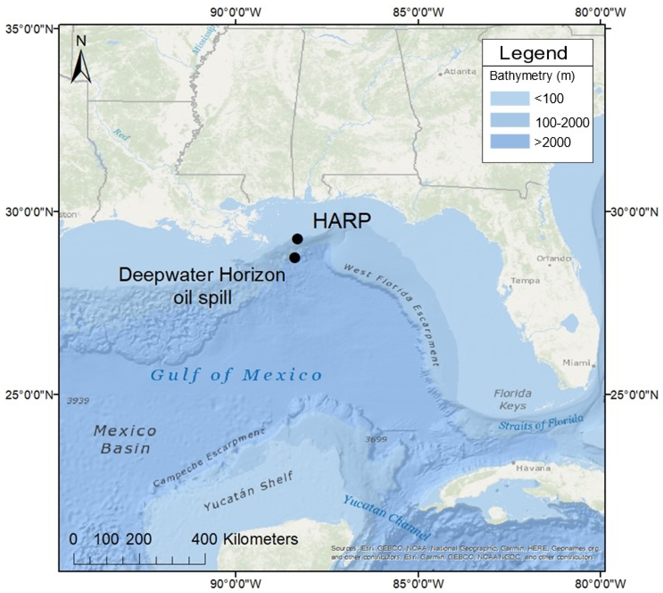
2.1. Data Collection

Data used for training, testing and evaluation of the detector and classifier were collected using a High-frequency Acoustic Recording Package (HARP), a bottom-mounted, autonomous calibrated recorder, containing a two-channel hydrophone—one to record high frequencies and one to record low frequencies (sensitivity: −200 dB re Vrms/µPa and −187 dB re Vrms/µPa, respectively; flat frequency response (±1.5 dB): 1–100 Hz and 1–10,000 Hz, respectively) [55]. The HARP was deployed in the northern Gulf of Mexico, approximately 60 km north of the 2010 Deepwater Horizon oil spill site, at ~90 m depth (Figure 1). Recordings were collected between 2010 and 2012 continuously, with short gaps for recovery and redeployment. The HARP recorded at a sample rate of 200 kHz with 16-bit quantization.
The data were pre-processed by converting the compressed binary files into WAV files. All WAV files were decimated to a sampling frequency of 2 kHz (initial sampling frequency: 200 kHz) to reduce the data to a 1 kHz bandwidth (0–1000 Hz), which allowed for faster computational analysis because the fish calls of interest have energy content below 1 kHz [25,30]. Long-Term Spectral Averages (LTSAs), with a frequency and temporal resolution of 1 Hz and 5 s, respectively, were calculated from the data using Triton, a Matlab-based acoustic analysis software package [56]. A years’ worth of data were manually analyzed to determine potential fish call types in the dataset. There were a total of six likely fish calls identified in these data that were the main target of this analysis. They are likely fish calls due to their low frequency (<1 kHz) and drumming or vibratory, pulsed sound [29,30,31]. The six calls varied in frequency and duration (Figure 2, Table 1). Five of the six calls—Beats, Buzz, Croak, Downsweep, and Pulse train—have not been documented before and are named based on the way they sound. It is possible the Jetski is the same call as the 300 Hz frequency modulated harmonic call described by Wall et al. [57]; however, it is difficult to discern based on the limited call description and low-resolution spectrogram.

2.2. Train/Test and Evaluation Datasets

When developing artificial intelligence methods to detect and classify calls, it is necessary to have two datasets: a train/test and evaluation dataset. A train/test dataset was established from one month of data (August 2010) and was used to develop and modify the automatic detector and classifier. This month was selected because all six fish call types were present, as well as many different noise types, and a relatively high number of occurrence of each call was present compared to other months that were manually analyzed. The evaluation dataset was composed of the first seven days of June, September, and December 2011 and March 2012, as well as 18–24 July 2012 to cover all four seasons, two different years, and provide a good number of all six call types. These data were used to assess the performance of the detector and classifier on a new, diverse subset of the long-term dataset.
Triton was used to manually create the groundtruth, a log of the six fish calls of interest, for both datasets. When signals of interest were visually detected in the Triton-generated LTSA (plot length: 1 h), a short, higher-resolution spectrogram (plot length: 30–120 s, Hanning window, 90% overlap, frequency resolution: 2 Hz, time resolution: 0.5 s) was used to identify the fish call and record the call’s start and end time. The average maximum and minimum frequencies and duration of each call type were measured, too (Table 1). Based on the analyst’s manual analysis, the train/test dataset contained a total of 834 calls of the six fish call types and the evaluation dataset contained a total of 1503 calls of the six fish call types.
Data analysis occurred in two steps—detection followed by classification. These two methods are explained in more detail in Section 2.3 and Section 2.4.

2.3. Call Detection: Energy Detector

To effectively and automatically determine the occurrence of signals of interest, fish calls were detected and extracted from the recording’s waveforms using the energy detector feature of Ishmael, a bioacoustics analysis software [58]. An energy detector was used to detect the six fish calls of interest because it is a general, broad detector, capable of detecting any signal or noise within a certain frequency band and above a specific threshold that the user specifies. The fish call characteristics needed to create the Ishmael energy detector were average minimum call frequency, average maximum call frequency, and average call duration (Table 1). The specified detector parameters included the frequency band (maximum frequency and minimum frequency), call duration, threshold, and call detection neighborhood, which is how soon a subsequent call can be detected after an initial detection. These parameters were iteratively adjusted until a detector with a high recall (>85%) was established for the train/test dataset. Because the energy detector did not rely on other temporal characteristics, such as amplitude, number of pulses, or interpulse interval, they were not measured for each call type and the focus of this paper is the application of automatic analysis methods to these data, not describing each call.
To begin, a single, broadband energy detector (frequency range: 100–800 Hz) was applied to the dataset. The frequency range, threshold, and call detection neighborhood were then slowly decreased to 500 Hz (spanning from 150 to 650 Hz), 0.054, and 4 s, respectively. Recall is the fraction of true positives divided by the sum of true positives and false negatives (i.e., the number of detections that are also found in the groundtruth divided by the total number of calls in the groundtruth) and precision is the fraction of true positives divided by the sum of true positives and false positives (i.e., the number of detections that are also found in the groundtruth divided by all detections). Even though recall was relatively high with these parameters, precision was low (Figure S1), so modifications were made to the energy detector. Instead of one single broadband (150 to 650 Hz) energy detector, a detector with three smaller bands was applied to the train/test dataset. However, after iteratively adjusting the three frequency band widths and settling on 200 to 240 Hz (captured Beats and Buzz calls), 450 to 600 Hz (captured Downsweep, Jetski, and Pulse train calls), and 870 to 950 Hz (captured Croak calls) for the bands, detector precision and recall decreased (Figure S2). Because both recall and precision decreased, the three-band energy detector was not tested on the evaluation dataset and the single broadband energy detector was determined to be the best detector to extract the six fish call types in this dataset.
The most efficient detector at extracting the six fish call types from the train/test dataset operated over 150 to 650 Hz and had maximum call duration of 15 s with 4 s detection neighborhood and a threshold of 0.054. The detector was then applied to the evaluation dataset to check its performance on a new, diverse dataset it had not been trained on. Recall and precision were calculated for different buffer lengths (tested between 3 and 6 s) to assess detector performance (Figure S1) [59]. Buffer length was used to evaluate detector performance to see how close a detection is to a manually selected call; if the buffer length was set to 3 s, then that means a detection occurred within 3 s of a manually logged call start time and the detection would be considered a true positive. Therefore, a longer buffer length will result in a higher recall rate because it increases the probability that a detected signal will be identified in the dataset (Figure S1). In this study, recall was prioritized over precision because the overall purpose of the detector was to extract the majority of calls of interest. Each energy detection was saved as an individual WAV file with the detection start time as the file’s name and the detection centered in the file. The second step of the process, classification, enabled rejection of the false detections and retention of signals of interest.

2.4. Call Classification: ResNet-50 Convolutional Neural Network

Before the classification step could be conducted, the automatic detections had to be converted into images. A custom-built MATLAB code was created to convert each Ishmael energy detection WAV file into an image (JPG file) by performing a short-time Fourier transform on each detection audio file, resulting in images with 2 Hz and 0.5 s resolution. Each detection WAV file was read into MATLAB and then a spectrogram of the detection file was created and changed to gray scale; the spectrogram was then filtered with a 2D Gaussian smoothing kernel with standard deviation of 1 and saved as an image.
Transfer learning was used to classify all of the detected images [60,61]. The pre-trained convolutional neural network that was used was ResNet-50 [62] and it was chosen because of its efficiency, accuracy, and simplicity to retrain for other classification purposes [63,64,65]. The classifier was trained with an unbalanced dataset since some fish calls were less common than others (Figure 3). The ~2200 image dataset (train/test image dataset) used to train and test ResNet-50 were images of the manually detected six fish call types from the August 2010 train/test dataset, as well as with images of five noise types—Disk write, Click train, Blank/noise (Blank), Low frequency noise (LF Noise), and Random noise (Ra Noise)—which were commonly observed in the dataset (Figure S3). Disk write is self-made noise by the HARP that occurs every 75 s. Click train most likely represents sounds produced by dolphins. LF Noise was most often airgun noise. Only 26 Downsweep fish calls were manually detected in the train/test dataset, so 27 additional Downsweep images, which were manually detected in the long-term dataset, were added to increase the number of Downsweep images to 53, and 32 manually detected Beats images from the evaluation dataset were added to increase the number of Beats images to 151.
ResNet-50′s accuracy was optimized by experimenting with data augmentation and adjusting hyperparameters, such as number of epochs and mini batch size. Data augmentation involved iteratively adjusting the scaling and translation range of images [66]. When using augmentation to train the classifier in this study, images were randomly scaled and translated by any value in the range specified by the user. In this study, the scale range was specified as ±10% in the Y dimension and the translation range was specified as ±50 pixels in the X dimension, meaning each individual training image was randomly scaled in just the Y dimension by any percentage between −10% and +10% and shifted to the left or right by any pixel value less than 51. However, it should be noted that there were probably instances where no scaling or no translation or neither augmentation parameter was applied since augmentation was random. For example, an image would only be translated if the random scaling value was 0%, or vice versa, an image would only be scaled randomly and not shifted if the random pixel translation value was 0, or the image would be scaled and translated, or both the scaling and translation values would be 0 so the image remained “unaugmented.” Therefore, classification accuracy can slightly differ between trials based on how the training images are randomly augmented. Images of the six fish call and five noise types were augmented (i.e., scaled and translated). The hyperparameters were set to 6 epochs and a mini batch size of 10.
Data augmentation was not used to adjust the level of background noise in the images. They already had various levels of background noise found in the data, ensuring the classifier was not trained on images with only the most intense and clear signals with low background noise. Lastly, the actual training dataset remained unbalanced after augmentation. Multiple epochs increased the training number of images for all sound types, so the classifier was trained on more images of the rarer call types (e.g., Downsweep and Pulse Train), but these rarer call types were not resampled more times than other call types to ensure equal numbers of images in the training process.
To examine classifier consistency and accuracy, the detection images from both datasets—train/test and evaluation—were run through the classifier three different times, so there were three classification trials for each dataset in order to calculate average recall and precision for each fish call type and to calculate average overall accuracy (total correctly labeled images/total number of images) for each dataset [53]. Recall and precision were also computed to assess classifier performance and a confusion matrix of classifier performance was used to evaluate accuracy for each trial and averaged for each dataset (Table 2, Table 3, Tables S1 and S2) [59]. For classification, recall is the fraction of correctly labeled images of one sound type divided by the total number of images of that one sound type and precision is the fraction of correctly labeled images of one sound type divided by the total number of images that are labeled as that one sound type. Accuracy is the fraction of true positives and true negatives divided by the total (i.e., total number of correctly labeled images in the dataset divided by the total number of images in the dataset). Lastly, to see if classifier performance could increase and further observe if the classifier was consistent in labeling images, detection images labeled as the six fish call types were re-classified because many images labeled as a fish call were often images of noise.
Finally, MATLAB was used to calculate the signal-to-noise ratio (SNR) of 100 randomly selected classified images of each fish call type—50 correctly classified and 50 incorrectly classified—to evaluate if classifier performance was dependent on the intensity of the signal compared to ambient background noise. To calculate SNR, the WAV file of each image was used and the frequency band and duration were adjusted for each call to capture where the most energy was present and to avoid including too much noise in the signal’s sound pressure level (SPL) calculation (Figure S4). Two SNR calculations were made for each Downsweep call because a high intensity version of the call would have multiple downsweeps present but a low intensity call, which was more commonly observed in the data, had one or two downsweeps; therefore, a full band SNR calculation would be quite low compared to the SNR calculation when just using the strongest downsweep. The SPL of the background noise, which was computed over the same frequency band and time duration as the signal SPL but prior to the start of the signal start time, was then subtracted from the signal SPL to compute the SNR. To analyze the SNR and classifier performance, binomial logistic regression was used (0 = call was misclassified, 1 = call was correctly classified) to fit a probability of correct classification curve. A threshold value of 0.5 was used to determine the SNR threshold value, which is the minimum SNR value beyond which calls have a chance better than random to be correctly classified (Figure S5). The area under the receiver operating characteristic curve (AUC) was then calculated to evaluate predictive performance of the logistic regression model (i.e., classifier performance based on the SNR of a call), where anything under 0.7 was bad, 0.7–0.8 was adequate, 0.8–0.9 was good, and >0.9 was excellent.

3. Results

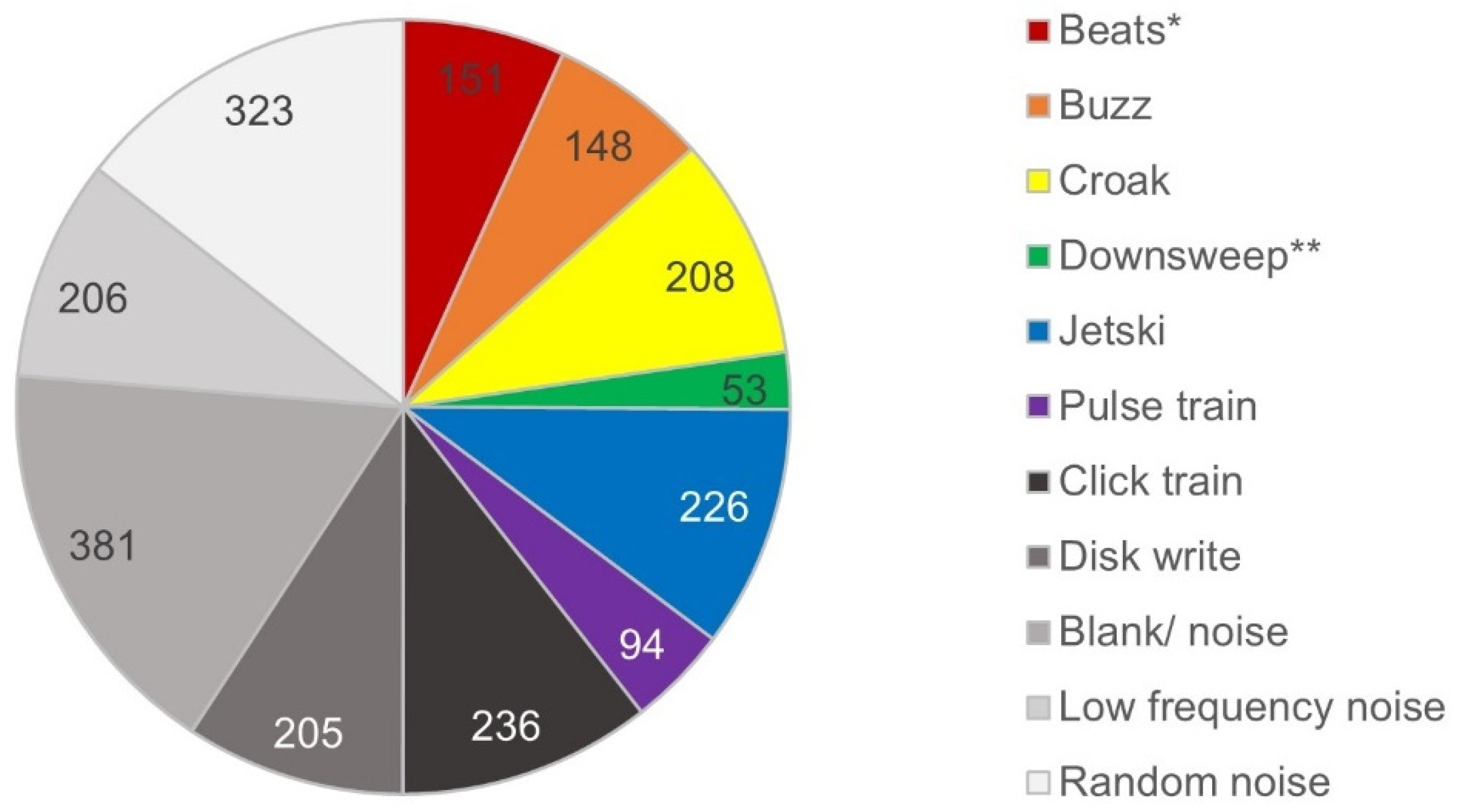
3.1. Energy Detector Performance

The energy detector recall ranged from 79 to 92% depending on the buffer length—as buffer length increased, so did recall (Figure S1a). Because detector recall was >85% when the buffer length was 4 s for the train/test dataset, the detector was also run on the evaluation dataset and recall only slightly decreased to 84.1% when buffer length was 4 s (Figure S1b).
Detector precision was very low (Figure S1). The detector extracted 91,387 and 128,938 signals of interest when applied to the train/test and evaluation datasets, respectively. Regardless of buffer length, detector precision was <1.2% for the train/test dataset and the evaluation dataset. Because the energy detector threshold was quite low, the detector selected all types of noise, including ships and boats, disk write, airguns, and a large variety of unidentified random noises (Figure S6).

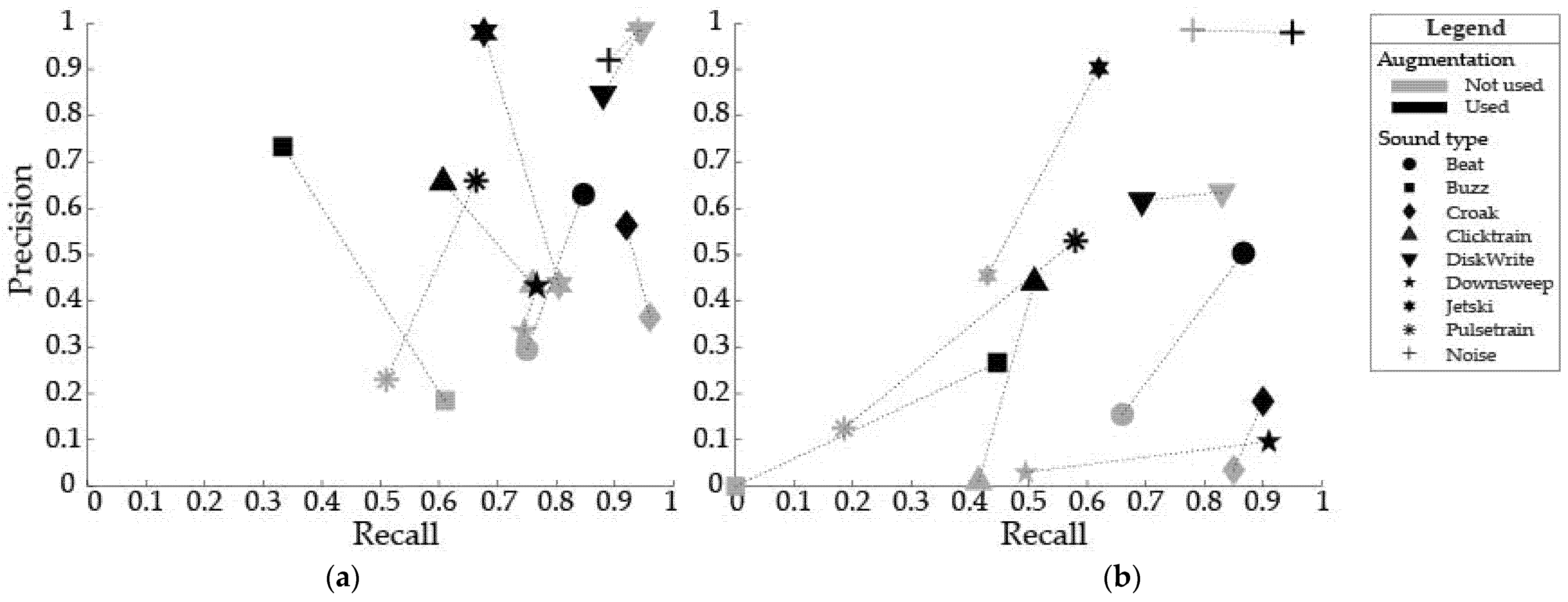
3.2. ResNet-50 Classifier Performance

Varying the training and testing set ratio (training: test ratio) of the train/test image dataset indicated that a higher training:test ratio increased classifier accuracy when labeling Downsweep images the most; for other call types, increasing the training:test ratio only slightly improved classifier accuracy (Figure S7). However, overall classification accuracy, the rate of correct classifications for all 11 sound types (not just the six fish calls), of the train/test image dataset increased when the training:test ratio increased. When the training:test ratio was 70:30, 80:20, and 90:10, overall accuracy was 90.5%, 91.4%, 95.1%, respectively. Therefore, a training:test ratio of 90:10 was used for the remainder of the study to train and then test ResNet-50′s performance prior to classifying the thousands of detection images from each dataset.
When augmentation was not used to train ResNet-50, average classifier precision was low for the six fish call types when classifying the train/test dataset (<45%) and evaluation dataset (<46%) (Figure 4). Because the six fish call types were not always in the same location in the detection image and call size (call duration and frequency band) would slightly vary, image augmentation was used to increase classifier precision. After iteratively adjusting the scaling factor and pixel translation range, classifier performance was highest when the scale range in only the Y dimension was ±10% and the translation range in only the X dimension was ±50 pixels. When these image augmentation settings were applied to images to train ResNet-50, as well as increasing the number of epochs to six so that the classifier looped through the train/test image dataset six times instead of just once, average classifier precision increased for all six fish call types (Figure 4). Augmentation also increased average classifier recall for all six fish call types when classifying the evaluation dataset detection images (Figure 4b). Even though average recall and precision varied greatly depending on fish call and noise type, average overall classifier accuracy with augmentation, when all 11 sound types are considered, was 87.97% and 93.02% for the train/test and evaluation dataset detection images, respectively (Table 2 and Tables S1 and S2).
Classifier performance varied among call types. The Buzz fish call had the lowest average recall rate (39.00%); most of the Buzz images were labeled as LF Noise, Blank, or Ra Noise (Table 3). For example, in one trial of the evaluation dataset, 61 of the 213 Buzz images were labeled correctly, 8 were labeled as another fish call type (Beats), and 144 were labeled as LF Noise, Blank, or Ra Noise. The other five fish call types had much higher average recall rates, from 91% for the Croak to 62% for the Pulse train (Table 3), than the Buzz call, but similar to the Buzz images, the majority of the other fish call images that were mislabeled were labeled as LF Noise, Blank, or Ra Noise, not as another fish call type (Tables S1 and S2).
A similar trend was observed for precision for all six fish call types—if images labeled as a fish call were misclassified, they were not commonly labeled as a different fish call type, but rather a noise type. For example, in one trial of the evaluation dataset, 1148 images were labeled as “Beats” of which 448 were Beats, but 663 were LF Noise, Blank, or Ra Noise, 5 were Disk Write, 6 were Click train, and 26 were other fish call types (21 of which were Buzz). The fish call type with the lowest average precision was Downsweep (26.50%) and the Croak fish call type had the second lowest average precision (37.33%) (Table 3). The four other fish call types had higher average precision (Beats: 56.67%, Buzz: 50.00%, Jetski: 94.17%, Pulse train: 59.50%). Interestingly, the average precision for each of the six call types for the evaluation dataset was lower than the train/test dataset average precisions for each of the fish calls.
Re-running the images labeled as any of the six fish calls through the classifier resulted in slightly (<0.5%) to greatly increased (>20%) classifier precision (Table 4). One train/test and evaluation data trial each had their percentage of correctly labeled images increase by <0.5%. On the other hand, two of the evaluation and one train/test dataset trials resulted in increases in precision between 19 and 34%, further indicating substantial level of the inconsistency in this classifier.
For all six fish call types, the SNR was not directly related to classifier performance (Figure S5). The selected SNR threshold value was greater than 0 for four of the calls (Beats, Buzz, Jetski, and Pulse train) and less than 0 for three of the calls (Croak, Downsweep full sweep, and Downsweep strongest sweep). For all fish calls, however, many calls were not correctly classified even when the SNR value was greater than the SNR threshold value. The area under the receiver operating characteristic curve (AUC) values ranged from 57.1% (Buzz) to 86.2% (Beats), indicating the logistic regression model ranged from “bad” to “good” (i.e., classifier performance was variable when labeling images correctly based on the SNR value), depending on the call type (Figure S5). Based on the model, classifier performance was “bad” at correctly labeling images of Buzz (57.1%), Croak (63.5%), Jetski (67.0%), and Pulse train (66.9%) calls based on their SNR, “adequate” at correctly labeling images of Downsweep calls when the full or strongest downsweep was measured (full: 76.6%; strongest: 71.8%), and “good” at correctly labeling images of Beats calls (86.2%).

3.3. Analysis Time: Manual vs. Automatic Methods

Using the energy detector and a pre-trained neural network sped up the call detection and identification process (Table 5). These automatic methods, implemented on a mid-range desktop computer with 8.00 GB RAM, 64-bit operating system, and Intel Core i3-8100 CPU and no GPU, resulted in processing of a month of data in approximately 8 and 10 hrs for the train/test and evaluation dataset, respectively. Manually going through a day of data takes 15 to 45 min depending on the number of calls present and amount of background noise. It took the analyst more than double the time (~2.6) to go through each dataset than the two-step automatic detection and classification methods applied in this study.

4. Discussion

We used an effective automatic detector and classifier system to efficiently extract and label six fish call types from a long-term passive acoustic monitoring dataset from the northern Gulf of Mexico. This approach offers the potential to expedite the analysis process for multiyear datasets from this region. However, understanding the caveats and potential pitfalls of the process is important before applying it to long-term data.

4.1. Automatic Energy Detector

The energy detector function in Ishmael was chosen since it is a general, broad detector capable of extracting the six fish call types, which vary in duration and frequency. The recall rate in this study (~85%) was similar to the recall rate in another fish acoustic study [46]. Ruiz-Blais et al. [46] used four Jamaica weakfish call features to create their detector, which had an accuracy of 96% and recall of 81%, and Monczak et al. [50] had a signal detector with an identification rate ((#files-# of files with false negative-# of files with false positive/#files)*100) > 80% in most cases, depending on species, recorder location, and call type. Wall et al. [67] developed an automatic detection algorithm to extract red grouper (Epinephelus morio) calls within a year-long dataset and its recall rate was 44%; however, they prioritized precision over recall because they were more interested in timing of sound production rather than call abundance. Ricci et al. [47] also used a detector to extract fish calls of interest, but they measured detector performance by the false detection rate (=1—precision); their false detection rate was ~1%, which is significantly higher than the rate observed for the energy detector in this study (precision < 1.2%). Additionally, two other studies [48,49] developed their own algorithm that both detected and identified their target fish call/s in their respective datasets. Kottege et al. [48] used spectro-temporal features to successfully identify tilapia calls with ~98% accuracy and a recall rate of 94%, using discriminant analysis methods. Chérubin et al. [49] did not report detector recall, but their algorithm had an overall identification accuracy of 87.5%; however, it varied based on species.
The majority of detections in our data were noise. The high false detection rate was not surprising because the Gulf of Mexico has one of the loudest US water soundscapes due to shipping and seismic exploitation and exploration, including airgun presence [68,69,70]. Manual review of detections revealed that many were airguns, which is not surprising since seismic surveys occur all year in the northern Gulf of Mexico. Another frequent detection was Disk write, which is self-made noise by the HARP; this noise occurs every 75 s and was often detected by the energy detector we developed.
Despite the low precision, the energy detector by itself was deemed a good detector since it had a relatively high recall rate and it resulted in more total detections of the six fish call types than the manual observer analysis, indicating that even though the detector did not detect all of the same fish calls as the analyst, it was capable of extracting the calls at alternate times that were missed by the analyst. It should be noted that in our analysis, when the detector extracted a signal of interest and the signal was a fish call that the manual observer had not marked, the detection was considered a false positive, even though a fish call was present. Any other treatment would have resulted in a bias in our analysis.
Lastly, the train/test (August 2010) and evaluation datasets were manually analyzed by three different people to reduce subjectivity and bias because there is often inconsistency in marking calls among multiple analysts [71]. Rather than combine the manual detections from all three observers, we chose to use only one analyst’s log as our groundtruth for both datasets because that log had more total fish calls marked and at the same time contained ~80% of the calls marked by the other two analysts. This approach led to a larger dataset for evaluation and, thus, higher detector precision and recall.

4.2. ResNet-50 Classifier

ResNet-50 is an efficient and accurate pre-trained neural network that can easily be retrained for other classification purposes [63,64]. Based on the literature review for this study, this is the only fish acoustic study to date that has used transfer learning to classify fish calls. Other fish acoustic studies used machine learning algorithms that were created and trained specifically to detect and classify their fish calls of interest [45,49,51,52,53,54,72]. Pre-trained neural networks that can be retrained for other classification purposes, such as AlexNet [73], GoogleNet [74], and ResNet-50, provide scientists, who have a background in biology and ecology rather than signal processing or artificial intelligence, with a ready-to-use model that can be easily modified based on their classification goals and target signal. Zhang et al. [75] observed that classification accuracy was >20% higher when they used transfer learning compared to training a neural network from the beginning on the 16 target whale calls in their dataset.
In this study, the classifier ResNet-50 was retrained with an unbalanced dataset of images of the six fish call types and five noise types that were commonly detected by the energy detector. The higher the training:test set ratio, the higher the classification accuracy for each of the six fish call types, especially Downsweep, which only had a total of 53 images for training and testing. It is well-known that classifier performance is frequently dependent on the size and quality of the training dataset [76]. Two fish acoustic studies that used automatic classification methods noted the impact of training set size. Harakawa et al. [51] used sequential machine learning algorithms to classify Sciaenidae calls and recall increased from 80.8% to 92.2% when the percentage of training data increased from 1% to 80%. Noda et al. [53] observed that median classification accuracy increased from 81.77% to 95.58% when the training dataset size increased from 5% to 50%. Both studies used a smaller training set percentage (<80% of the train/test image dataset) than what we used (90%), but the number of images they had for their calls of interest was greater than the number of images we had for each category, which is why our train:test ratio was larger than normal.
Image augmentation, as well as having a mini batch size of 10 and 6 epochs increased classifier precision across all fish call types (Figure 4). Interestingly, none of the fish acoustic studies to date (according to our literature search) mentioned using image augmentation to train their classifier; however, image augmentation has been used to increase the training data size and classification performance when labeling other animal calls [75,77,78]. For example, Padovese et al. [79] used image augmentation to generate synthetic calls to increase training data size resulting in increased classifier recall and precision for labeling North Atlantic right whale (Eubalaena glacialis) upcalls. Rasmussen and Širović [80] used scaling and translation augmentation to prevent their classifier from overfitting during the training process. Image augmentation was beneficial in this study because the number of images for training and testing was relatively small (<400 images) for each sound type; in fact, two of the six fish calls had <100 images each for training and testing (Figure 3). Therefore, increasing the number of epochs and using augmentation to scale and translate images increased the training set size and ensured the classifier was trained on images where the call or noise was not always in the same location in the image and the size of each call and noise was slightly variable.
The fish call types with the lowest (39.00%) and highest (91.00%) average recall was Buzz and Croak, respectively. Usually, classifier performance is lower for short-duration, pulsed calls [45,52]; however, classifier recall did not appear to depend on call duration or frequency band in our study. For the two pulsed calls, Pulse train and Downsweep, average recall was 62.17% (second lowest, but much higher than average recall for Buzz) for Pulse train and 83.83% (third highest) for Downsweep. Additionally, it was surprising that the Buzz had a low average recall because calls with distinguished harmonics had a higher identification rate (i.e., classified correctly more often) than shorter duration, pulsed calls in another fish acoustic study [50]. It is likely Buzz calls were misclassified because they slightly resemble airguns (LF Noise; Figure S6c) and Ra Noise, which have more energy (i.e., higher intensity) at very low frequencies (<100 Hz) similar to the Buzz call (Figure 2b). Average classifier recall was lower than might be expected for relatively long-duration Jetski calls (64.83%). They were often labeled as Blank, which was surprising because upon reviewing the images, the call was always present and visible.
Average precision of the classifier, on the other hand, generally appeared related to call duration or frequency band for most of the fish calls. Even though average recall was not the highest for the Jetski call (third lowest, 64.83%), average precision was much higher for the Jetski call (94.17%) than the other five fish call types (second highest, Pulse train: 59.50%). This is likely because the Jetski call looks unique and does not resemble any of the other calls or noise, making it easy to distinguish from the other call and noise types (Figure 2e). The Downsweep call had the lowest average precision (26.50%); most images labeled as “Downsweep” were noise, but Jetski and Pulse train images were also labeled as Downsweep occasionally because some Jetski calls are short in duration and may resemble a Downsweep. Pulse train calls are pulsed calls that are in the same frequency band as the strongest sweep in a Downsweep call (Figure 2d,f) which could also have contributed to the confusion. Croak had the second lowest average precision (37.33%) with images of broadband noise and Disk write, which loosely look like the Croak call, commonly labeled as “Croak.” The presence of airguns also impacted precision. They are low frequency noise and cover the same frequency band as Beats and Buzz [69,70] and could have been the cause of reduced precision for those calls, because lots of LF Noise was labeled as Beats and Buzz. Further, because there was greater airgun presence in the evaluation dataset than the train/test dataset, average precision for Beats and Buzz was further lowered in the evaluation dataset. Lastly, average recall was higher than average precision for four of the six calls—Beats, Croak, Downsweep, Pulse train. Harakawa et al. [51] similarly noted that overall classifier recall was greater than overall classifier precision, regardless of training set size, when classifying Sciaenidae calls.
Finally, average overall classifier accuracy in this study (~90%) was similar to classifier accuracies observed in fish acoustic studies that used automatic analysis methods, such as matched filters and machine learning algorithms [49,50,52,53,72,81]. Some studies with higher performance trained their models on fewer classes (i.e., sound types). ResNet-50 was trained on 11 sound types (six fish calls and five common noises) and other studies have shown that more classes (referred to as sound types in this study) often result in lower classification accuracy [45,82]. When Vieira et al. [45] used four sound types of meagre calls, the overall mean identification rate was 43.3%, but when they reduced the number of sound types to two, the overall mean identification rate increased to 78.8%. Maintaining a large number of classification labels can be useful for datasets with a large variety of signals and when the focus of the study is not a single species or sound source. ResNet-50 performed well overall in this study and was capable at labeling 11 different sound types and thus could be a good option for other studies of multiple sound sources as well. Interestingly, the “SNR” of each image (each spectrogram had to be converted into an image to be processed by the ResNet-50 classifier) did not appear to affect classifier accuracy (Figure S5). The relatively gradual logistic curve, low AUC values, and many calls that were not correctly classified even though they had a high SNR indicate the poor predictive performance of the logistic regression model and that SNR does not appear to affect classification performance (i.e., accuracy) in this study. This was unexpected since the SNR affected automatic detection and classification of fish chorusing and individual calls in other studies [53,54]. However, both Noda et al. [53] and Lin et al. [54] ran their detection and classification algorithm on spectrograms instead of images, which means that signal intensity and frequency influence detection and classification differently than 2D images [83]. Overall, though, ResNet-50 classified images of the six fish call types well, regardless of the SNR.

4.3. Considerations for Application of This Approach to Long-Term Datasets

There is no ideal or standard way to divide all available data between training/testing and evaluation. However, typical studies split the data so that 70–80% is used for training and testing the model and 20–30% is used for evaluating how the model performs on data it has not seen before. In this study, though, we used a much larger evaluation dataset than typical (~55% of the data). To apply this two-step methodology to real data, we thought it was important to evaluate the detector and classifier performance across a variety of situations, including different months, seasons, years, and noise levels (e.g., airgun and shipping presence). Therefore, a large evaluation dataset was specifically used to ensure that the energy detector and ResNet-50 could perform as well across a large variety of sound conditions that represent the diverse soundscape of the northern Gulf of Mexico.
The coupled automatic detector and machine learning methodology used in this study expedites the call detection and identification process when analyzing a long-term passive acoustic monitoring dataset. The analyst took ~2.6 more time to analyze each dataset than the automatic methods used in this study, and this difference in analysis time could be further increased if a supercomputer with more specialized and powerful hardware, such as RAM, GPU, and FPGA, is used [84]. However, already, the methods employed here could produce results on fish call presence from a full year of acoustic data in about five days of processing time. The energy detector feature in Ishmael and ResNet-50 are relatively simple programs that can be easily modified to detect and classify any signal, or signals, of interest without requiring extensive programming abilities or equipment. Further, this study is proof of concept that transfer learning can be used in fish vocalization studies, which has not been applied in any previous fish acoustic study.
Even though the classifier performed well overall (~90% accuracy), it is important to note the inconsistency in classifier performance. The accuracies of the three trials for each dataset were similar to each other (Table 2); however, the recall and precision for each fish call varied among trials for each dataset, indicating that the classifier was not consistent at labeling images (Table 3). Further, when we re-ran the images labeled as any of the six fish calls, the percentage of correctly labeled images increased between 0.2% and 34.3% for the six trials (Table 4). This broad range in percentage of correctly re-classified images originally labeled as a fish call shows the inconsistency in classifier performance. However, seeing an increase of >19% in the percentage of correctly re-labeled images for three of the six trials also suggests that using the classifier multiple times can ultimately lead to improvement in the overall output (i.e., accuracy and precision). However, this multiple-classification process may need to be coupled with a manual review step to validate fish detections and remove misclassified noise from the final output.
This methodology could be applied to datasets with multiple call types that have diverse, variable temporal features. In our study, temporal variations in calls did not matter because the energy detector will pick up any signal if it is above the specified threshold and within the specified frequency band; the number of pulses and interpulse interval did not affect detection recall and precision. Similarly, since our training dataset represented the variability of calls’ temporal features, the success of the classifier was not affected by those variations. For example, images labeled as Beats had from one to more than five Beats present with calls separated or overlapping. Additionally, images with three to seven pulses for a Pulse train were reliably identified as a Pulse train due to their short duration and relative y-position in the image (i.e., frequency), regardless of the interpulse interval. Therefore, as long as the training set is diverse and fairly large (or diversified and expanded with the use of data augmentation), the methods used in this study can detect and classify calls well, even when there are temporal and frequency variations. The energy detector is broad and can work for any signals of interest, while the pre-trained ResNet-50 classifier could work with any call type. However, for different call types, a separate library of training and test images will have to be developed and ResNet-50 will have to be retrained for those particular calls for the classifier to work on the new call types.
The methods developed in this study have the potential to be applied to soundscapes and signals from a variety of ecosystems. By decimating the data, we were able to remove from the energy detection most of the higher frequency biological noise—snapping shrimp and cetaceans—that is also abundant in the region. A similar decimation approach might be of use to others wishing to reduce false detections in the first step of the process. Our study region, the Gulf of Mexico, is one of the loudest U.S. water soundscapes [69] with high levels of low-frequency anthropogenic noise (e.g., commercial shipping and airguns). These sounds could not be removed by decimation since they generally overlap in frequency with our calls of interest. Even with these noises, however, our methods performed well because the six fish call types were common in the dataset, allowing development of a robust training and testing library, and distinct from other sounds in the environment. In most instances, automated detection and classification should be used on signals that are relatively common and easy to distinguish. In cases of sounds that are rare or whose features are challenging to distinguish, it is not likely any automated classification methods will perform satisfactorily. Therefore, the methodology presented in this paper should be well suited for relatively common signals, regardless of habitat type and levels of noise present, be they biophonic, anthrophonic, or geophonic.
In conclusion, this two-step process presents a novel, effective method to study soniferous fish abundance and presence and can help ecologists and managers understand potential population recovery based on call numbers and change in occurrence patterns over the years. As the next step, the energy detector and ResNet-50 classifier will be applied to the long-term PAM dataset collected between August 2010 and August 2017 at this location in the Gulf of Mexico. Those results will enable us to estimate changes in call abundance and observe daily, monthly, and annual calling patterns in the area, and possibly assess the impact of the 2010 Deepwater Horizon oil spill on the local fish community.

Supplementary Materials

The following are available online at https://www.mdpi.com/article/10.3390/jmse9101128/s1, Table S1: Average confusion matix of the three train/test dataset trials, Table S2: Average confusion matrix of the three evaluation dataset trials, Figure S1: Energy detector precision and recall dependent on various buffer lengths (3 s, 4 s, 5 s, and 6 s) for: (a) the train/test dataset and (b) the evaluation dataset, Figure S2: Comparison of precision and recall between the three-band detector (circles) and single, broadband (stars) energy detector based on various buffer lengths of 3 s, 4 s, 5 s, and 6 s, Figure S3: Images (created from spectrograms) of the five noise types that the classifier was trained with: (a) Disk write, (b) Click train, (c) Blank/ noise, (d) Low frequency noise, (e) Low frequency noise, (f) Random noise, and (g) Random noise, Figure S4: Images (created from spectrograms) of the six fish call types: (a) Beats, (b) Buzz, (c) Croak, (d) Downsweep full sweep, (e) Downsweep strongest sweep, (f) Jetski, and (g) Pulse train, with shaded bands (yellow) representing the frequency band and duration over which the signal sound pressure level was calculated for each call type. Two SNR calculations were made for each Downsweep call (indicated by d and e) because a high intensity Downsweep call had multiple downsweeps, but a less intense Downsweep call, which was more commonly observed in the data, had only one or two downsweeps, Figure S5: Binomial logistic regression plots with a 0.5 threshold (black, dotted horizontal line; 0 = incorrectly classified, 1 = correctly classified) to determine the signal-to-noise ratio (SNR) threshold value (vertical blue line in each subplot), the SNR value above which a call should be correctly classified, for each fish call type: (a) Beats, (b) Buzz, (c) Croak, (d) Downsweep full sweep, (e) Downswee strongest sweep, (f) Jetski, and (g) Pulse train. Area under the receiver operating characteristic curve J. Mar. Sci. Eng. 2021, 9, x FOR PEER REVIEW 16 of 19 (AUC) calculation included in each subplot for each fish call type, Figure S6: Images (created from spectrograms) of commonly detected noises in the three datasets: (a) ship noise, (b) disk write, (c) airguns, (d) airguns, (e) unidentified noise, and (f) unidentified noise, Figure S7: ResNet-50 classification accuracy for each of the six fish call types depending on the training:test set ratio (30:70, 50:50, 70:30, 80:20, 90:10).

Author Contributions

Conceptualization, A.Š. and E.E.W.; methodology, A.Š. and E.E.W.; software and coding, E.E.W. and J.H.R.; validation, E.E.W.; formal analysis, E.E.W.; data curation, A.Š.; writing—original draft preparation, E.E.W.; writing—review and editing, A.Š. and J.H.R.; visualization, E.E.W.; supervision, A.Š.; project administration, A.Š.; funding acquisition, A.Š. All authors have read and agreed to the published version of the manuscript.

Funding

This research was funded by the NRDA partners and BP, award number 20105138, as well as C-IMAGE and C-IMAGE II under grants from The Gulf of Mexico Research Initiative.

Institutional Review Board Statement

Not applicable.

Informed Consent Statement

Not applicable.

Data Availability Statement

The data presented in this study are available on request from the corresponding author. The data are not publicly available due to large size.

Acknowledgments

We would like to acknowledge past and present members of the Scripps Whale Acoustics Lab at the Scripps Institution of Oceanography for HARP deployment and recovery, as well as Hannah Bassett and Sarah Johnson, who initially selected the six fish calls of interest studied in this paper. We also want to acknowledge Steve Murawski and Sherryl Gilbert at the University of San Francisco of C-IMAGE for their support for acoustic work.

Conflicts of Interest

The authors declare no conflict of interest. The funders had no role in the design of the study; in the collection, analyses, or interpretation of data; in the writing of the manuscript, or in the decision to publish the results.

References

  1. Fine, M.L.; Thorson, R.F. Use of Passive Acoustics for Assessing Behavioral Interactions in Individual Toadfish. Trans. Am. Fish. Soc. 2008, 137, 627–637. [Google Scholar] [CrossRef]
  2. Blumstein, D.T.; Mennill, D.; Clemins, P.; Girod, L.; Yao, K.; Patricelli, G.; Deppe, J.L.; Krakauer, A.; Clark, C.; Cortopassi, K.A.; et al. Acoustic monitoring in terrestrial environments using microphone arrays: Applications, technological considerations and prospectus. J. Appl. Ecol. 2011, 48, 758–767. [Google Scholar] [CrossRef]
  3. Wrege, P.H.; Rowland, E.D.; Keen, S.; Shiu, Y. Acoustic monitoring for conservation in tropical forests: Examples from forest elephants. Methods Ecol. Evol. 2017, 8, 1292–1301. [Google Scholar] [CrossRef]
  4. Linke, S.; Gifford, T.; Desjonquères, C.; Tonolla, D.; Aubin, T.; Barclay, L.; Karaconstantis, C.; Kennard, M.; Rybak, F.; Sueur, J. Freshwater ecoacoustics as a tool for continuous ecosystem monitoring. Front. Ecol. Environ. 2018, 16, 231–238. [Google Scholar] [CrossRef]
  5. Lammers, M.O.; Brainard, R.E.; Au, W.W.L.; Mooney, T.A.; Wong, K.B. An ecological acoustic recorder (EAR) for long-term monitoring of biological and anthropogenic sounds on coral reefs and other marine habitats. J. Acoust. Soc. Am. 2008, 123, 1720–1728. [Google Scholar] [CrossRef] [PubMed] [Green Version]
  6. Dede, A.; Öztürk, A.A.; Akamatsu, T.; Tonay, A.M.; Öztürk, B. Long-term passive acoustic monitoring revealed seasonal and diel patterns of cetacean presence in the Istanbul Strait. J. Mar. Biol. Assoc. United Kingd. 2014, 94, 1195–1202. [Google Scholar] [CrossRef]
  7. Nelson, D.V.; Garcia, T.S.; Klinck, H. Seasonal and Diel Vocal Behavior of the Northern Red-Legged Frog, Rana aurora. Northwestern Nat. 2017, 98, 33–38. [Google Scholar] [CrossRef]
  8. Palmer, K.J.; Brookes, K.L.; Davies, I.M.; Edwards, E.; Rendell, L. Habitat use of a coastal delphinid population investigated using passive acoustic monitoring. Aquat. Conserv. Mar. Freshw. Ecosyst. 2019, 29, 254–270. [Google Scholar] [CrossRef] [Green Version]
  9. Kalan, A.K.; Piel, A.K.; Mundry, R.; Wittig, R.M.; Boesch, C.; Kühl, H.S. Passive acoustic monitoring reveals group ranging and territory use: A case study of wild chimpanzees (Pan troglodytes). Front. Zool. 2016, 13, 34. [Google Scholar] [CrossRef] [PubMed] [Green Version]
  10. Riera, A.; Pilkington, J.; Ford, J.; Stredulinsky, E.; Chapman, N. Passive acoustic monitoring off Vancouver Island reveals extensive use by at-risk Resident killer whale (Orcinus orca) populations. Endanger. Species Res. 2019, 39, 221–234. [Google Scholar] [CrossRef]
  11. Ricci, S.; Eggleston, D.; Bohnenstiehl, D. Use of passive acoustic monitoring to characterize fish spawning behavior and habitat use within a complex mosaic of estuarine habitats. Bull. Mar. Sci. 2017, 93, 439–453. [Google Scholar] [CrossRef]
  12. Tricas, T.; Boyle, K. Acoustic behaviors in Hawaiian coral reef fish communities. Mar. Ecol. Prog. Ser. 2014, 511, 1–16. [Google Scholar] [CrossRef] [Green Version]
  13. Wilson, K.C.; Semmens, B.X.; Pattengill-Semmens, C.V.; McCoy, C. Potential for grouper acoustic competition and parti-tioning at a multispecies spawning site off Little Cayman, Cayman Islands. Mar. Ecol. Prog. Ser. 2020, 634, 127–146. [Google Scholar] [CrossRef] [Green Version]
  14. Celis-Murillo, A.; Deppe, J.L.; Allen, M.F. Using soundscape recordings to estimate bird species abundance, richness, and composition. J. Field Ornithol. 2009, 80, 64–78. [Google Scholar] [CrossRef]
  15. Deichmann, J.L.; Hernández-Serna, A.; Delgado C., J.A.; Campos-Cerqueira, M.; Aide, T.M. Soundscape analysis and acoustic monitoring document impacts of natural gas exploration on biodiversity in a tropical forest. Ecol. Indic. 2017, 74, 39–48. [Google Scholar] [CrossRef] [Green Version]
  16. Frommolt, K.-H. Information obtained from long-term acoustic recordings: Applying bioacoustic techniques for monitoring wetland birds during breeding season. J. Ornithol. 2017, 158, 659–668. [Google Scholar] [CrossRef]
  17. Širović, A.; Cutter, G.R.; Butler, J.L.; Demer, D.A. Rockfish sounds and their potential use for population monitoring in the Southern California Bight. ICES J. Mar. Sci. 2009, 66, 981–990. [Google Scholar] [CrossRef] [Green Version]
  18. Piercy, J.; Codling, E.; Hill, A.; Smith, D.; Simpson, S. Habitat quality affects sound production and likely distance of detection on coral reefs. Mar. Ecol. Prog. Ser. 2014, 516, 35–47. [Google Scholar] [CrossRef] [Green Version]
  19. Butler, J.; Stanley, J.A.; Butler, M.J., IV. Underwater soundscapes in near-shore tropical habitats and the effects of envi-ronmental degradation and habitat restoration. J. Exp. Mar. Biol. Ecol. 2016, 479, 89–96. [Google Scholar] [CrossRef]
  20. Hildebrand, J.A.; Frasier, K.E.; Baumann-Pickering, S.; Wiggins, S.M.; Merkens, K.P.; Garrison, L.P.; Soldevilla, M.S.; McDonald, M.A. Assessing Seasonality and Density From Passive Acoustic Monitoring of Signals Presumed to be From Pygmy and Dwarf Sperm Whales in the Gulf of Mexico. Front. Mar. Sci. 2019, 6, 66. [Google Scholar] [CrossRef] [Green Version]
  21. Wiggins, S.M.; Hildebrand, J.A. Long-term monitoring of cetaceans using autonomous acoustic recording packages. In Listening in the Ocean; Springer: Berlin/Heidelberg, Germany, 2016; pp. 35–59. [Google Scholar]
  22. Pirotta, E.; Brookes, K.L.; Graham, I.M.; Thompson, P.M. Variation in harbour porpoise activity in response to seismic survey noise. Biol. Lett. 2014, 10, 20131090. [Google Scholar] [CrossRef] [Green Version]
  23. Marcoux, M.; Ferguson, S.H.; Roy, N.; Bedard, J.; Simard, Y. Seasonal marine mammal occurrence detected from passive acoustic monitoring in Scott Inlet, Nunavut, Canada. Polar Biol. 2017, 40, 1127–1138. [Google Scholar] [CrossRef]
  24. Van Opzeeland, I.; Hillebrand, H. Year-round passive acoustic data reveal spatio-temporal patterns in marine mammal community composition in the Weddell Sea, Antarctica. Mar. Ecol. Prog. Ser. 2020, 638, 191–206. [Google Scholar] [CrossRef] [Green Version]
  25. Rountree, R.A.; Gilmore, R.G.; Goudey, C.A.; Hawkins, A.D.; Luczkovich, J.J.; Mann, D.A. Listening to fish: Applications of passive acoustics to fisheries science. Fisheries 2006, 31, 433–446. [Google Scholar] [CrossRef]
  26. Luczkovich, J.J.; Mann, D.A. and Rountree, R.A. Passive acoustics as a tool in fisheries science. Trans. Am. Fish. Soc. 2008, 137, 533–541. [Google Scholar] [CrossRef] [Green Version]
  27. Slabbekoorn, H.; Bouton, N.; van Opzeeland, I.; Coers, A.; Cate, C.T.; Popper, A.N. A noisy spring: The impact of globally rising underwater sound levels on fish. Trends Ecol. Evol. 2010, 25, 419–427. [Google Scholar] [CrossRef] [PubMed] [Green Version]
  28. Fish, M.P.; Mowbray, W.H. Sounds of Western North Atlantic Fishes: A Reference File of Biological Underwater Sounds; Johns Hopkins Press: Baltimore, MD, USA, 1970. [Google Scholar]
  29. Fine, M.L.; Parmentier, E. Mechanisms of fish sound production. In Sound Communication in Fishes; Ladich, F., Ed.; Springer: Berlin/Heidelberg, Germany, 2015; pp. 77–126. [Google Scholar]
  30. Amorim, M.C.P. Diversity of sound production in fish. Commun. Fishes 2006, 1, 71–104. [Google Scholar]
  31. Kasumyan, A.O. Sounds and sound production in fishes. J. Ichthyol. 2008, 48, 981–1030. [Google Scholar] [CrossRef]
  32. Ladich, F. Agonistic behaviour and significance of sounds in vocalizing fish. Mar. Freshw. Behav. Physiol. 1997, 29, 87–108. [Google Scholar] [CrossRef]
  33. Mann, D.A.; Lobel, P.S. Passive acoustic detection of sounds produced by the damselfish, Dascyllus albisella (Pomacentridae). Bioacoustics 1995, 6, 199–213. [Google Scholar] [CrossRef]
  34. Locascio, J.V.; Burton, M.L. A passive acoustic survey of fish sound production at Riley’s Hump within Tortugas South Ecological Reserve; implications regarding spawning and habitat use. Fish. Bull. 2016, 114, 103–116. [Google Scholar] [CrossRef]
  35. Lowerre-Barbieri, S.K.; Barbieri, L.R.; Flanders, J.R.; Woodward, A.G.; Cotton, C.F.; Knowlton, M.K. Use of Passive Acoustics to Determine Red Drum Spawning in Georgia Waters. Trans. Am. Fish. Soc. 2008, 137, 562–575. [Google Scholar] [CrossRef]
  36. Pieretti, N.; Martire, M.L.; Farina, A.; Danovaro, R. Marine soundscape as an additional biodiversity monitoring tool: A case study from the Adriatic Sea (Mediterranean Sea). Ecol. Indic. 2017, 83, 13–20. [Google Scholar] [CrossRef]
  37. Buscaino, G.; Ceraulo, M.; Pieretti, N.; Corrias, V.; Farina, A.; Filiciotto, F.; Maccarrone, V.; Grammauta, R.; Caruso, F.; Giuseppe, A.; et al. Temporal patterns in the soundscape of the shallow waters of a Mediterranean marine protected area. Sci. Rep. 2016, 6, 34230. [Google Scholar] [CrossRef] [Green Version]
  38. Lindseth, A.V.; Lobel, P.S. Underwater soundscape monitoring and fish bioacoustics: A review. Fishes 2018, 3, 36. [Google Scholar] [CrossRef] [Green Version]
  39. McCauley, R.D.; Cato, D.H. Patterns of fish calling in a nearshore environment in the Great Barrier Reef. Philos. Trans. R. Soc. Lond. Ser. B Biol. Sci. 2000, 355, 1289–1293. [Google Scholar] [CrossRef] [PubMed]
  40. Gavrilov, A.N.; McCauley, R.D.; Gedamke, J. Steady inter and intra-annual decrease in the vocalization frequency of Antarctic blue whales. J. Acoust. Soc. Am. 2012, 131, 4476–4480. [Google Scholar] [CrossRef] [PubMed] [Green Version]
  41. Zhang, Y.-J.; Huang, J.-F.; Gong, N.; Ling, Z.-H.; Hu, Y. Automatic detection and classification of marmoset vocalizations using deep and recurrent neural networks. J. Acoust. Soc. Am. 2018, 144, 478–487. [Google Scholar] [CrossRef]
  42. Salamon, J.; Bello, J.P.; Farnsworth, A.; Robbins, M.; Keen, S.; Klinck, H.; Kelling, S. Towards the Automatic Classification of Avian Flight Calls for Bioacoustic Monitoring. PLoS ONE 2016, 11, e0166866. [Google Scholar] [CrossRef]
  43. Mac Aodha, O.; Gibb, R.; Barlow, K.E.; Browning, E.; Firman, M.; Freeman, R.; Harder, B.; Kinsey, L.; Mead, G.R.; Newson, S.E.; et al. Bat detective—Deep learning tools for bat acoustic signal detection. PLoS Comput. Biol. 2018, 14, e1005995. [Google Scholar] [CrossRef] [PubMed] [Green Version]
  44. Bittle, M.; Duncan, A. A review of current marine mammal detection and classification algorithms for use in automated passive acoustic monitoring. In Proceedings of the Acoustics, Victor Harbor, Australia, 17–20 November 2013. [Google Scholar]
  45. Vieira, M.; Pereira, B.P.; Pousão-Ferreira, P.; Fonseca, P.J.; Amorim, M.C.P.; Ferreira, P. Seasonal Variation of Captive Meagre Acoustic Signalling: A Manual and Automatic Recognition Approach. Fishes 2019, 4, 28. [Google Scholar] [CrossRef] [Green Version]
  46. Ruiz-Blais, S.; Camacho, A.; Rivera-Chavarria, M.R. Sound-based automatic neotropical sciaenid fishes identification: Cynoscion jamaicensis. In Proceedings of the Meetings on Acoustics 167th ASA, Acoustical Society of America, Providence, RI, USA, 5–9 May 2014. [Google Scholar]
  47. Ricci, S.W.; Bohnenstiehl, D.R.; Eggleston, D.B.; Kellogg, M.L.; Lyon, R.P. Oyster toadfish (Opsanus tau) boatwhistle call detection and patterns within a large-scale oyster restoration site. PLoS ONE 2017, 12, e0182757. [Google Scholar] [CrossRef] [PubMed] [Green Version]
  48. Kottege, N.; Kroon, F.; Jurdak, R.; Jones, D. Classification of underwater broadband bio-acoustics using spectro-temporal features. In Proceedings of the Seventh ACM International Conference on Underwater Networks and Systems, Los Angeles, CA, USA, 5–6 November 2012; pp. 1–8. [Google Scholar]
  49. Chérubin, L.M.; Dalgleish, F.; Ibrahim, A.K.; Schärer-Umpierre, M.; Nemeth, R.S.; Matthews, A.; Appeldoorn, R. Fish Spawning Aggregations Dynamics as Inferred from a Novel, Persistent Presence Robotic Approach. Front. Mar. Sci. 2020, 6, 779. [Google Scholar] [CrossRef]
  50. Monczak, A.; Ji, Y.; Soueidan, J.; Montie, E.W. Automatic detection, classification, and quantification of sciaenid fish calls in an estuarine soundscape in the Southeast United States. PLoS ONE 2019, 14, e0209914. [Google Scholar] [CrossRef]
  51. Harakawa, R.; Ogawa, T.; Haseyama, M. and Akamatsu, T. Automatic detection of fish sounds based on multi-stage classi-fication including logistic regression via adaptive feature weighting. J. Acoust. Soc. Am. 2018, 144, 2709–2718. [Google Scholar] [CrossRef]
  52. Vieira, M.; Fonseca, P.J.; Amorim, M.C.P.; Teixeira, C.J.C. Call recognition and individual identification of fish vocalizations based on automatic speech recognition: An example with the Lusitanian toadfish. J. Acoust. Soc. Am. 2015, 138, 3941–3950. [Google Scholar] [CrossRef]
  53. Noda, J.J.; Travieso, C.M.; Sánchez-Rodríguez, D. Automatic Taxonomic Classification of Fish Based on Their Acoustic Signals. Appl. Sci. 2016, 6, 443. [Google Scholar] [CrossRef] [Green Version]
  54. Lin, T.-H.; Tsao, Y.; Akamatsu, T. Comparison of passive acoustic soniferous fish monitoring with supervised and unsu-pervised approaches. J. Acoust. Soc. Am. 2018, 143, EL278–EL284. [Google Scholar] [CrossRef]
  55. Wiggins, S.M.; Hildebrand, J.A. High-frequency Acoustic Recording Package (HARP) for broad-band, long-term marine mammal monitoring. In Proceedings of the 2007 Symposium on Underwater Technology and Workshop on Scientific Use of Submarine Cables and Related Technologies, Tokyo, Japan, 17–20 April 2007; pp. 551–557. [Google Scholar]
  56. Wiggins, S.M.; Roch, M.A.; Hildebrand, J.A. TRITON software package: Analyzing large passive acoustic monitoring data sets using MATLAB. J. Acoust. Soc. Am. 2010, 128, 2299. [Google Scholar] [CrossRef]
  57. Wall, C.; Lembke, C.; Mann, D. Shelf-scale mapping of sound production by fishes in the eastern Gulf of Mexico, using autonomous glider technology. Mar. Ecol. Prog. Ser. 2012, 449, 55–64. [Google Scholar] [CrossRef] [Green Version]
  58. Mellinger, D. Ishmael: 1.0 User’s Guide; Ishmael: Integrated System for Holistic Multi-Channel Acoustic Exploration and Localization; NOAA Technical Memorandum OAR PMEL-120: Newport, OR, USA, 2002; Volume 30, p. 2434.
  59. Sirović, A. Variability in the performance of the spectrogram correlation detector for North-east Pacific blue whale calls. Bioacoustics 2016, 25, 145–160. [Google Scholar] [CrossRef]
  60. Caruana, R. Learning many related tasks at the same time with backpropagation. In Proceedings of the Advances in Neural Information Processing Systems, Denver, CO, USA, 28 November–1 December 1994; pp. 657–664. [Google Scholar]
  61. Bengio, Y. Deep learning of representations for unsupervised and transfer learning. In Proceedings of the ICML Workshop on Unsupervised and Transfer Learning, JMLR 27 Workshop and Conference Proceedings, Bellevue, WA, USA, 2 July 2011; pp. 17–37. [Google Scholar]
  62. He, K.; Zhang, X.; Ren, S.; Sun, J. Deep residual learning for image recognition. In Proceedings of the IEEE Conference on Computer Vision and Pattern Recognition, Las Vegas, NV, USA, 27–30 June 2016; pp. 770–778. [Google Scholar]
  63. Sharma, N.; Jain, V.; Mishra, A. An analysis of convolutional neural networks for image classification. Procedia Comput. Sci. 2018, 132, 377–384. [Google Scholar] [CrossRef]
  64. Rauf, H.T.; Lali, M.I.U.; Zahoor, S.; Shah, S.Z.H.; Rehman, A.U.; Bukhari, S.A.C. Visual features based automated identi-fication of fish species using deep convolutional neural networks. Comput. Electron. Agric. 2019, 167, 105075. [Google Scholar] [CrossRef]
  65. Raikar, M.M.; Meena, S.M.; Kuchanur, C.; Girraddi, S.; Benagi, P. Classification and Grading of Okra-ladies finger using Deep Learning. Procedia Comput. Sci. 2020, 171, 2380–2389. [Google Scholar] [CrossRef]
  66. Bianco, M.J.; Gerstoft, P.; Traer, J.; Ozanich, E.; Roch, M.A.; Gannot, S.; Deledalle, C.-A. Machine learning in acoustics: Theory and applications. J. Acoust. Soc. Am. 2019, 146, 3590–3628. [Google Scholar] [CrossRef] [PubMed] [Green Version]
  67. Wall, C.; Simard, P.; Lindemuth, M.; Lembke, C.; Naar, D.; Hu, C.; Barnes, B.B.; Muller-Karger, F.E.; Mann, D. Temporal and spatial mapping of red grouper Epinephelus morio sound production. J. Fish. Biol. 2014, 85, 1470–1488. [Google Scholar] [CrossRef]
  68. Haver, S.M.; Gedamke, J.; Hatch, L.T.; Dziak, R.P.; Van Parijs, S.; McKenna, M.F.; Barlow, J.; Berchok, C.; DiDonato, E.; Hanson, B.; et al. Monitoring long-term soundscape trends in U.S. Waters: The NOAA/NPS Ocean Noise Reference Station Network. Mar. Policy 2018, 90, 6–13. [Google Scholar] [CrossRef]
  69. Wiggins, S.M.; Hall, J.M.; Thayre, B.J.; Hildebrand, J.A. Gulf of Mexico low-frequency ocean soundscape impacted by airguns. J. Acoust. Soc. Am. 2016, 140, 176–183. [Google Scholar] [CrossRef] [Green Version]
  70. Estabrook, B.; Ponirakis, D.; Clark, C.; Rice, A. Widespread spatial and temporal extent of anthropogenic noise across the northeastern Gulf of Mexico shelf ecosystem. Endanger. Species Res. 2016, 30, 267–282. [Google Scholar] [CrossRef] [Green Version]
  71. Baumgartner, M.F.; Mussoline, S.E. A generalized baleen whale call detection and classification system. J. Acoust. Soc. Am. 2011, 129, 2889–2902. [Google Scholar] [CrossRef] [Green Version]
  72. Malfante, M.; Mars, J.I.; Mura, M.D.; Gervaise, C. Automatic fish sounds classification. J. Acoust. Soc. Am. 2018, 143, 2834–2846. [Google Scholar] [CrossRef] [PubMed] [Green Version]
  73. Krizhevsky, A.; Sutskever, I.; Hinton, G.E. ImageNet classification with deep convolutional neural networks. Adv. Neural. Inf. Process. Syst. 2012, 25, 1097–1105. [Google Scholar] [CrossRef]
  74. Szegedy, C.; Liu, W.; Jia, Y.; Sermanet, P.; Reed, S.; Anguelov, D.; Erhan, D.; Vanhoucke, V.; Rabinovich, A. Going deeper with convolutions. In Proceedings of the IEEE Conference on Computer Vision and Pattern Recognition, Boston, MA, USA, 7–12 June 2015; pp. 1–9. [Google Scholar]
  75. Zhang, L.; Wang, D.; Bao, C.; Wang, Y.; Xu, K. Large-Scale Whale-Call Classification by Transfer Learning on Multi-Scale Waveforms and Time-Frequency Features. Appl. Sci. 2019, 9, 1020. [Google Scholar] [CrossRef] [Green Version]
  76. Kavzoglu, T. Increasing the accuracy of neural network classification using refined training data. Environ. Model. Softw. 2009, 24, 850–858. [Google Scholar] [CrossRef]
  77. Nanni, L.; Maguolo, G.; Paci, M. Data augmentation approaches for improving animal audio classification. Ecol. Inform. 2020, 57, 101084. [Google Scholar] [CrossRef] [Green Version]
  78. Vickers, W.; Milner, B.; Lee, R. Improving the robustness of right whale detection in noisy conditions using denoising autoencoders and augmented training. In Proceedings of the 2021 IEEE International Conference on Acoustics, Speech and Signal Processing (ICASSP), Toronto, ON, Canada, 6–11 June 2021; pp. 91–95. [Google Scholar] [CrossRef]
  79. Padovese, B.; Frazao, F.; Kirsebom, O.S.; Matwin, S. Data augmentation for the classification of North Atlantic right whales upcalls. J. Acoust. Soc. Am. 2021, 149, 2520–2530. [Google Scholar] [CrossRef]
  80. Rasmussen, J.H.; Širović, A. Automatic detection and classification of baleen whale social calls using convolutional neural networks. J. Acoust. Soc. Am. 2021, 149, 3635–3644. [Google Scholar] [CrossRef]
  81. Ibrahim, A.K.; Zhuang, H.; Chérubin, L.M.; Schärer-Umpierre, M.T.; Erdol, N. Automatic classification of grouper species by their sounds using deep neural networks. J. Acoust. Soc. Am. 2018, 144, EL196–EL202. [Google Scholar] [CrossRef] [Green Version]
  82. Strukova, O.V.; Myasnikov, E.V. The choice of methods for the construction of PCA-based features and the selection of SVM parameters for person identification by gait. J. Phys. Conf. Ser. 2019, 1368, 032001. [Google Scholar] [CrossRef]
  83. Wyse, L. Audio spectrogram representations for processing with convolutional neural networks. In Proceedings of the First International Workshop on Deep Learning and Music, joint with IJCNN, Anchorage, AK, USA, 17–18 May 2017; pp. 37–41. [Google Scholar]
  84. Zhang, Q.; Zhang, M.; Chen, T.; Sun, Z.; Ma, Y.; Yu, B. Recent advances in convolutional neural network acceleration. Neurocomputing 2019, 323, 37–51. [Google Scholar] [CrossRef] [Green Version]
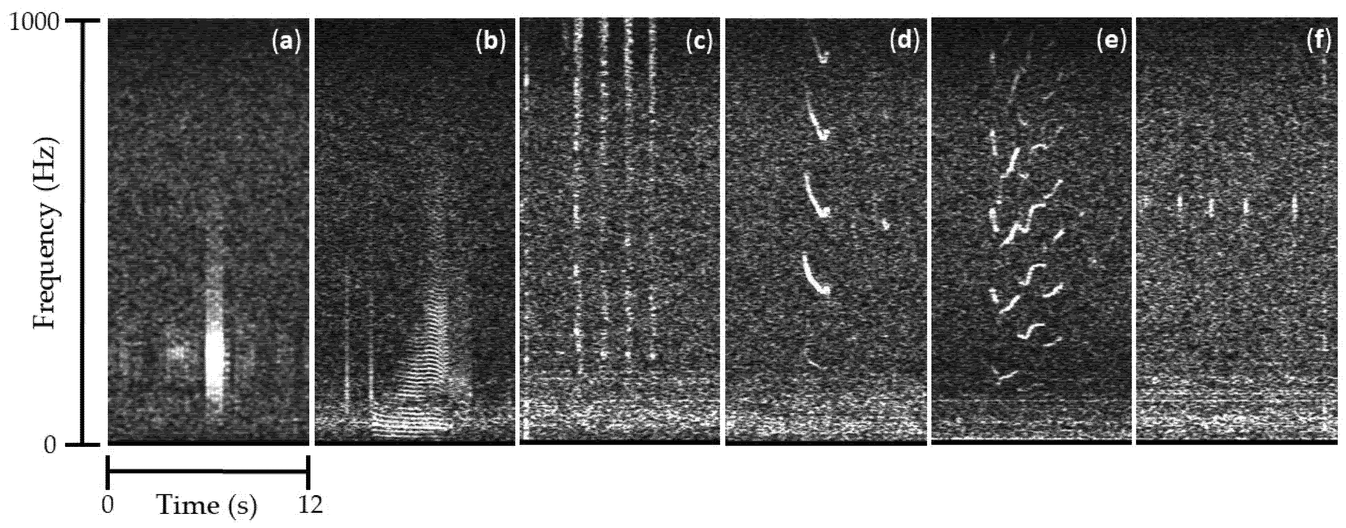
Figure 1. High-frequency acoustic recording package (HARP) deployment location in the northern Gulf of Mexico.
Jmse 09 01128 g001
Figure 2. Images (created from spectrograms) of the six potential fish calls from the northern Gulf of Mexico recording location: (a) Beats, (b) Buzz, (c) Croak, (d) Downsweep, (e) Jetski, and (f) Pulse train. Time and frequency scaling are provided for a better sense of the call’s characteristics. The scaling and gray scale are the same for all images.
Jmse 09 01128 g002
Figure 3. The number of images from the August 2010 train/test dataset used to train and test the classifier ResNet-50 for each sound type, including the six fish call types (colored; Beats, Buzz, Croak, Downsweep, Jetski, and Pulse train) and five noise types (gray scale; Click train, Disk write, Blank/noise, Low frequency noise, and Random noise). The total number of images for training and testing was 2231, with more than half of the images representing a noise type. * Majority of Beats calls were from August 2010 train/test dataset, but 32 were from the evaluation dataset. ** Approximately half of the Downsweep images were from the August 2010 train/test dataset and the other half was from other periods in the long-term dataset.
Jmse 09 01128 g003
Figure 4. Average (n = 3) classifier precision and recall with and without image augmentation (black and light gray shapes, respectively) to train the classifier. Results are presented when classifying: (a) the ~91,300 train/test dataset detection images and (b) the ~129,000 evaluation dataset detection images. Three noise categories (Low Frequency Noise, Blank/noise, and Random Noise) are combined to make the figures more clear.
Jmse 09 01128 g004
Table 1. Frequency (average minimum and maximum) and temporal (average, maximum, and minimum duration) characteristics of the six fish call types based on 30 randomly selected calls of each call type.
Call TypeAverage Minimum
Frequency (Hz)
Average Maximum
Frequency (Hz)
Average Duration (s)Maximum Duration (s)Minimum Duration (s)
Beats1212741.82.51.1
Buzz353436.218.02.2
CroakNANA10.592.82.6
Downsweep3108501.94.81.0
Jetski2148025.111.72.8
Pulse train46156323.5101.44.9
Table 2. Overall classifier accuracy (total correctly labeled detection images/total detection images) for the three different times (i.e., three trials) all the detection images from both datasets—train/test and evaluation—were classified by the data-augmented, trained classifier, as well as the average overall classifier accuracy for each dataset.
DatasetTrial #Overall Classifier Accuracy (%)Average Overall Accuracy (%)
August 2010 Train/test187.4287.97
288.20
388.29
Evaluation193.8793.02
293.82
391.35
Table 3. The average recall and precision rate (%) for each of the six fish call types for each dataset and the combined average recall and precision for each call type when considering all six trials (three train/test and three evaluation). The average precision and recall values for each call come from Tables S1 and S2 for the train/test and evaluation dataset, respectively.
DatasetBeatsBuzzCroakDownsweepJetskiPulse Train
Recall (%)Precision (%)Recall (%)Precision (%)Recall (%)Precision (%)Recall (%)Precision (%)Recall (%)Precision (%)Recall (%)Precision (%)
August 2010 Train/test84.6763.0033.3373.3392.0056.3376.6743.3367.6798.0066.3366.00
Evaluation86.6750.3344.6726.6790.0018.3391.009.6762.0090.3358.0053.00
Combined (Average)85.6756.6739.0050.0091.0037.3383.8326.5064.8394.1762.1759.50
Table 4. Reclassification statistics including the total number of detection images, the number of detection images labeled as a fish call, the number (and percentage) of correctly classified detection images, and the number (and percentage) of correctly re-classified detection images for the three trials for each dataset.
DatasetTrial #Total
Detection Images
Detection
Images Labeled as a Call
# Correctly
Classified Images
# Correctly
Re-Classified Images
Aug 2010 Train/test191,38736471902 (52.2%)2617 (71.8%)
291,38724291751 (72.1%)1759 (72.4%)
391,38728111814 (64.5%)2042 (72.6%)
Evaluation1128,93834131538 (45.1%)1546 (45.3%)
2128,93849871605 (32.2%)3318 (66.5%)
3128,93873471717 (23.4%)5352 (45.2%)
Table 5. Statistics on detector and classifier performance including the number of recording days, the number of detections selected by the energy detector, the amount of time (hr:min) it took the detector to run, the average amount of time it took the classifier to label the detection images from each dataset, and the amount of time it took the analyst to manually annotate each dataset.
DatasetNumber of Recording DaysTotal
Detection Images
Time to Run Detector (hr:min)Average Time to Run Classifier (hr:min)Manual Analysis Time (hr:min)
Aug 2010 Train/Test3191,3874:104:0721:35
Evaluation35128,9383:506:0926:20
Publisher’s Note: MDPI stays neutral with regard to jurisdictional claims in published maps and institutional affiliations.

