Coupled SPH–FEM Modeling of Tsunami-Borne Large Debris Flow and Impact on Coastal Structures

Abstract

Field surveys in recent tsunami events document the catastrophic effects of large waterborne debris on coastal infrastructure. Despite the availability of experimental studies, numerical studies investigating these effects are very limited due to the need to simulate different domains (fluid, solid), complex turbulent flows and multi-physics interactions. This study presents a coupled SPH–FEM modeling approach that simulates the fluid with particles, and the flume, the debris and the structure with mesh-based finite elements. The interaction between the fluid and solid bodies is captured via node-to-solid contacts, while the interaction of the debris with the flume and the structure is defined via a two-way segment-based contact. The modeling approach is validated using available large-scale experiments in the literature, in which a restrained shipping container is transported by a tsunami bore inland until it impacts a vertical column. Comparison of the experimental data with the two-dimensional numerical simulations reveals that the SPH–FEM models can predict (i) the non-linear transformation of the tsunami wave as it propagates towards the coast, (ii) the debris–fluid interaction and (iii) the impact on a coastal structure, with reasonable accuracy. Following the validation of the models, a limited investigation was conducted, which demonstrated the generation of significant debris pitching that led to a non-normal impact on the column with a reduced contact area and impact force. While the exact level of debris pitching is highly dependent on the tsunami characteristics and the initial water depth, it could potentially result in a non-linear force–velocity trend that has not been considered to date, highlighting the need for further investigation preferably with three-dimensional models.

1. Introduction

After the Indian Ocean Tsunami in 2004 and Great East Japan Tsunami in 2011, which resulted in significant destruction of coastline infrastructure and enormous financial losses [1], tsunamis have gained a great deal of attention. Due to the enormous amount of energy, tsunami waves can travel many kilometers and pose significant threats to coastal communities, taking away lives, and causing serious damage to coastal structures. In spite of the low frequency of the occurrence of such events, due to population growth, the urbanization trend and sea level rise, the exposure of coastal environments to extreme water hazards is increasing. Past tsunamis revealed that much of the nearshore infrastructure located in tsunami-prone areas is highly vulnerable to hydrodynamic loads. Extensive damage to coastal buildings, bridges, seawalls, and breakwaters was reported after the 2004 Indian tsunami and the 2011 Tohoku tsunami [2,3,4,5]. FEMA P-646 [3] reported that the Indian tsunami generated by a Mw9.1 subduction earthquake [3] caused extensive damage to critical infrastructure and total loss of life over 310,000 [6]. Flooding caused by the 2011 Tohoku tsunami affected areas that were 7 miles away from the shore and damaged over 162,000 buildings and more than 300 bridges [5,6,7,8,9].

Several numerical simulations and experimental studies have been carried out to date to advance the understanding of tsunami forces on coastal structures. Palermo et al. [10] described the tsunami-induced force components on nearshore structures and reported that the hydrodynamic and surge components were a function of the instantaneous velocity and water depth. Other studies focused on the experimental testing of tsunami bore loads on rectangular buildings [11], piloti-type buildings [12], walls with overhangs [13] and coastal bridges [14,15,16,17]. Some studies evaluated the effects of different wave forms on coastal decks, including unbroken, breaking and post-breaking waves and bores [14,18], and revealed fundamental differences in the effects caused by the two wave types. In fact, Istrati et al. [18] demonstrated that turbulent bores applied horizontal forces that were larger than the uplift forces by up to a factor of 2.2, while the unbroken waves exhibited an opposite trend with a ratio of horizontal/uplift force decreasing down to 0.54. This highlighted the need to be able to identify a priori the tsunami wave type that is expected to impact a specific coastal area in order to design properly a new structure or strengthen an existing one at that location. Fortunately, several simplified predictive load equations have been developed in the literature for a range of different types of structures, for both bores [19,20] and unbroken solitary waves [21,22].

Other critical aspects related to the hydrodynamic effects on coastal structures that have been identified by previous studies include the high aleatory variability of bore impact on structures [13,17], the importance of structural flexibility and dynamic fluid–structure interaction [17,23,24], the critical role of trapped air below elevated decks [21,25,26,27,28] and the demand on individual connections and columns [29]. For example, Robertson et al. [13] found a significant variability in the impulsive uplift pressures applied by a turbulent bore on the slab soffit of a vertical wall with an overhang, with the maximum pressures at selected locations ranging between 3 and 7.5 kPa among the different repetitions of the same bore. Similarly, Istrati [17] showed a large aleatory variability in the bore-induced horizontal force on a bridge deck with the standard deviation in the experimental tests being equal to approximately 20% of the average value. However, after the decomposition of the total force into a slamming and quasi-static component, it was revealed that the variability is generated by the slamming component. Moreover, several studies found that the air entrapment below elevated decks with girders can significantly increase the maximum total uplift forces generated by solitary waves [21,30]. However, the trapped air can also increase the overturning moment, while it has a complex and inconsistent effect on the total slamming and on the uplift demand in the offshore bearings and columns generated by bores [28].

In addition to the adverse tsunami-induced effects on coastal structures documented by the aforementioned studies focusing on ‘clear-water’ conditions, field surveys after recent tsunamis revealed the presence of waterborne debris (e.g., containers, cars, wooden poles), which can result in an increase in the uplift and drag forces and lead to significant lateral displacement and potential instability of the structure [1,31,32]. Consequently, the quantification of the impact forces caused by the waterborne debris attracted the attention of several research studies, both numerical [33,34,35] and experimental [36,37,38,39]. According to Haehnel and Daly [36], the peak debris impact force is a function of the impact velocity, the mass of the debris, and the effective stiffness. Como and Mahmoud [35] evaluated the debris impact on interior and exterior wood structural panels using fluid–structure interaction analyses and reported that the debris impact forces on an exterior panel increased with the wave height, while this was not the case for the interior panels. Ko [37] investigated experimentally the impact of a shipping container on a column and reported that the in-water applied load was 1.2-fold larger than the corresponding in-air condition, and had a longer duration. An equation to estimate the debris velocity based on the relative distance of debris pick-up location and the structure was developed in Shafiei et al. [38]. Derschum et al. [40] investigated the debris impact on structures and reported that the initial impoundment depth had a significant effect on the impact angle. Moreover, the same study observed a non-linear movement of the debris with a reduced impact velocity close to the structure, which was attributed to the formation of splitting streamlines and a stagnation zone in front of the coastal structure.

Yang [41] studied the tsunami-induced debris loading on bridge decks using the material point method. The results of the analyses showed that the presence of debris increases the applied loads on bridges, with the in-water analyses giving up to 35% larger debris impact forces than the in-air cases. Oudenbroek et al. [42] carried out an experimental and numerical study to evaluate the failure mechanism of selected bridges in Japan. The results confirmed that debris accumulation had significant effects on the hydraulic demand on bridges by increasing the uplift and drag forces, which could lead to the structural failure of the bridge. Istrati et al. [43] carried out a three-dimensional (3D) numerical investigation on the effects of tsunami-borne debris damming on coastal bridges. The results demonstrated that a shipping container trapped below the offshore overhang of a bridge has a negligible effect on the horizontal load but it can increase the overturning moment (pitching), which could consequently increase the probability of failure of the offshore bearings and connections that have to withstand this moment. If the container is trapped at locations offset from the mid-length of the span (e.g., close to the supports of the span), significant yaw and roll moments are generated due to 3D effects, which could lead to unequal distribution of the loads to the structural components of the two bent caps or abutments.

The majority of the numerical studies conducted to date on tsunami and extreme flooding effects on structures used mesh-based solvers that employed the finite volume [26,42] or the finite element method [23,44], while some of them used particle-based methods including smoothed particle hydrodynamics [45,46,47] or hybrid particle-finite methods such as PFEM [48]. SPH is a Lagrangian-based meshless technique, in which continuum properties of the fluid are discretized by a set of non-connected particles that carry individual material properties describing the medium, including, position, velocity, mass, density, pressure, and other physical quantities [49]. The Lagrangian nature of the SPH makes this method well suited to problems with large deformations and distorted free surface. The major advantage of using SPH is in dealing with free-surface problems where there is no need for special treatments for the free surface in order to simulate highly non-linear and potentially violent flows [50]. In recent years, SPH has been widely utilized to simulate a wide range of coastal and ocean engineering applications, such as solitary waves on beaches [51], breaking waves [52,53,54,55], wave–structure interaction and impact on coastal structures [45,46,47,56,57,58,59,60], and wave overtopping on offshore platforms [61]. Although the SPH method is one of the most matured forms of meshless techniques for cases of large deformations, such as during the breaking process of a wave, the computational accuracy and efficiency in simulating small deformation of solid bodies are lower than that of the FEM approach [62]. However, in the context of coastal structures and their dynamic response to large wave loads, the hybrid SPH–FEM approach could be utilized to take advantages of the ability of: (a) the SPH method to simulate complex free-surface flows and large fluid deformations, and (b) the FEM to simulate the dynamics of the structure [63,64].

The number of available numerical studies of tsunami-borne debris loading on coastal structures is quite limited, which can be attributed to the challenging multi-physics nature of the phenomenon. This phenomenon involves a complex fluid flow with turbulent wave breaking, a non-linear debris–fluid interaction with large deformations, a contact between the debris, the fluid and the coastal structure, and a dynamic structural response. Given (i) the catastrophic effects of large tsunami-borne debris, such as containers, in past tsunami events, and (ii) the good performance of SPH in other coastal engineering applications, the aim of this manuscript is to present a coupled SPH–FEM numerical modeling approach and evaluate its accuracy in simulating both the debris flow and the impact on a coastal structure. Therefore, this paper presents first a detailed explanation of the governing equations and modeling approach. Then, a comprehensive comparison of the coupled SPH–FEM models against experimental data available in the literature [37,65] is presented in terms of wave propagation and tsunami inland flow, debris motion and impact on a downstream coastal structure. Following the verification phase, a preliminary investigation focusing on the role of the debris restraints, the tsunami characteristics, and the initial water depth is conducted in order to shed light on the underlying physics of the debris–fluid interaction and impact on structures, and identify some critical parameters that govern this complex phenomenon.

2. Numerical Method

The SPH technique employed in this research is available in LS-DYNA [66] and is based on weakly compressible smoothed particle hydrodynamics (WCSPH). Several numerical investigations of fluid–structure interaction (FSI) were conducted using the SPH formulation in LS-DYNA to study large deformation problems [55,65,67]. For example, Pelfrene [55] used the SPH method for the simulation of free-surface water flow with focus on regular and breaking wave, and found that the solver is able to simulate the free-surface flow and capture the main features of the plunging breaking wave. Moreover, Grimaldi et al. [67] and Panciroli et al. [68] used the same method to investigate the impact of a solid body on water and both of them showed a good comparison with experimental results, justifying the selection of this solver for the numerical investigation conducted in the current study.

2.1. SPH Governing Equations

2.1.1. Kernel Approximation

In the SPH method, the particles are the computational framework on which the governing equations are resolved. This method is based on a quadrature formula on moving particles. Traditional SPH formulation exhibits very substantial pressure oscillation when modelling fluid flow. Instead of using the traditional computational grid, the conservation laws of continuum mechanics are defined by partial equations. For any SPH pseudo-particle, the function describing the field Ω is approximated in the form of a “kernel function”, which is stated as the integral form of the product of any function and kernel function [66,69]:

$$<f\left(x\right)>={\int }_{\Omega }f\left(x^{\prime }\right)W\left(x-x^{\prime },h\right){dx}^{\prime },$$

(1)

where $x$ and $x^{\prime }$ are the position vectors of the material points in a domain Ω;$f\left(x\right)$ is the continuous function of the field corresponding to the coordinate $x;f\left(x^{\prime }\right)$ is the value of quantity at the point $x^{\prime }$; $W\left(x-x^{\prime },h\right)$ is the bell-shaped smooth kernel function, where $h$ is the smoothing length, defining the influence volume of the smooth function which varies in time and in space.

The smoothing function determines the range of computation with other particles and therefore has a significant effect on precision and accuracy of the analyses. The kernel function can be constructed taking in account a number of conditions and should satisfy the following properties [49]:

• The smoothing function is normalized:

$${\int }_{\Omega }W\left(x-x^{\prime },h\right){dx}^{\prime }=1,$$

(2)

2.

There is a compact support for the smoothing function:

$$W\left(x-x^{\prime },h\right) =0, for \left|x-x^{\prime }\right| >\kappa h,$$

(3)

where $\kappa$ is the constant that determines the effective area of the smoothing function. This area is called the support domain.

3.

$W\left(x-x^{\prime },h\right)$ is non-negative for any $x^{\prime }$ within the support domain. This is necessary to achieve physically meaningful results in hydrodynamic computations.

4.

The smoothing length increases as particles separate and reduces as the concentration increases.

5.

With the smoothing length approaching zero, the kernel approaches the Dirac delta function:

$$\underset{h\to 0}{\lim }W\left(x-x^{\prime },h\right) =\partial \left(x-x^{\prime }\right),$$

(4)

6.

The smoothing function should be an even function.

The forms of kernel functions usually include a quantic spline function [70], a cubic spline function [71] and a Gaussian kernel function [72]. By balancing the calculation accuracy and efficiency and considering that the commercial software LS-DYNA was used for the simulations throughout this study, the following B-spline smoothing function was adopted [66]:

$$W\left(x,h\right)=\frac{1}{h{\left(x\right)}^d}\theta \left(x\right),$$

(5)

where d is the number of space dimensions (2 or 3) and $\theta \left(x\right)$ is the cubic B-spline function defined by:

$$\theta (\mathrm{x})=C\ast \left\{\begin{array}{l}1-\frac{3}{2}{x}_{xj}^2+\frac{3}{4}{x}_{xj}^3\hspace{1em} for\hspace{1em} x_{ij}\le 1\\ \frac{1}{4}(2-x_{ij}{)}^3\hspace{1em} for\hspace{1em} 1<x_{ij}\le 2\\ 0\hspace{1em} for\hspace{1em} 2<x_{ij}\end{array}\right.$$

(6)

where C is a constant for normalization, depending on the number of space dimensions and $x_{ij}$ is the relative distance of particles i and j.

2.1.2. Particle Approximation

The second key aspect in SPH formulations is the particle approximation, which enables the system to be represented by a finite number of particles that carry an individual mass and occupy an individual space. For the SPH method, Equation (1) can be transformed into discretized forms by summing up the values of the field function within the support domain defined by the smoothing length $h$ as follows [69]:

$$<f\left(x_i\right)>={\sum }_{j=1}^n\frac{m_{j }}{{\rho }_j}f\left(x_i\right) W(x_i-x_j,h)={\sum }_{j=1}^n\frac{m_{j }}{{\rho }_j}f\left(x_j\right) W_{ij},$$

(7)

where $<f\left(x_i\right)>$ is the kernel approximation operator; $f\left(x_j\right)$ is the physical value at the jth position, $i$ is the number of any particle in the domain; $n$ is the total number of particles within the influence area of the particle $i$; and $m_j$ and ${\rho }_j$ are the mass and density associated with particle j. Thus, the value of particle $i$ is approximated using the weighted average of the function values at all particles within the support domain of particle $j$. The partial approximation of the spatial derivation of a function can be expressed as in Das and Holm [73]:

$$<\nabla .f\left(x_i\right)> ={\sum }_{j=1}^n\frac{m_{j }}{{\rho }_j}f\left(x_i\right). \nabla W_{ij},$$

(8)

where

$$\nabla W_{ij}=\frac{x_{i }-x_{j }}{r_{ij}}\frac{\partial W_{ij}}{\partial r_{ij}}$$

(9)

2.2. SPH for Viscous Fluid

The smoothing kernel and particle approximation can be used for discretization of partial differential equations (PDEs). The SPH formulation is derived by discretizing the Navier–Stokes equations spatially, thus leading to a set of ODEs which can be solved via time integration. Substituting the SPH approximations for a function and its derivative to the partial differential equations governing the physics of fluid flows, the discretization of these governing equations can be written as follows [74]:

$$\begin{gathered} \frac{d{\rho }_i}{dt}={\sum }_{j=1}^n m_{j } (x_i^{\beta }-x_j^{\beta }) \frac{\partial W_{ij}}{\partial x_i^{\beta }}, \\ \frac{d{v}_i^{\alpha }}{dt}={\sum }_{j=1}^n m_{j } (\frac{{\sigma }_i^{\alpha \beta }}{{\rho }_i^2}+\frac{{\sigma }_j^{\alpha \beta }}{{\rho }_j^2})\frac{\partial W_{ij}}{\partial x_i^{\beta }}, \\ \frac{d{v}_i^{\alpha }}{dt}={\sum }_{j=1}^n m_{j } (\frac{{\sigma }_i^{\alpha \beta }}{{\rho }_i{\rho }_j}.\frac{\partial W_{ij}}{\partial x_i^{\beta }}-\frac{{\sigma }_j^{\alpha \beta }}{{\rho }_i{\rho }_j}.\frac{\partial W_{ij}}{\partial x_j^{\beta }}), \\ \frac{d{e}_i}{dt}=-\frac{p_i+{\Pi }_{ij}}{{\rho }_i^2}{\sum }_{j=1}^n m_{j } (v_i-v_j) \frac{\partial W_{ij}}{\partial x_i^{\beta }}, \\ \frac{d{x}_i^{\alpha }}{dt}=v_i+\epsilon {\sum }_{j=1}^n \frac{m_{j } }{{\rho }_j}(v_i-v_j) W_{ij}, \end{gathered}$$

(10)

where the superscripts $\alpha$ and $\beta$ are the coordinate directions; g is the acceleration of gravity;$\sigma$ is the particle stress; $v$ is the particle velocity; $e$ is the internal energy per unit mass; $\epsilon$ is the shear strain rate ($\epsilon$ $\cong 0.5)$ and ${\Pi }_{ij}$ is the Monaghan artificial viscosity [75]. In the analysis of the interaction between waves and structures, ${\Pi }_{ij}$ can prevent the non-physical shock of the solution results in the impact area and effectively prevent the non-physical penetration of particles when they are close to each other. The role of artificial viscosity is to smoothen the shock over several particles and to allow the simulation of viscous dissipation, the transformation of kinetic energy to heat. Therefore, to consider the artificial viscosity, an artificial viscous pressure term ${\Pi }_{ij}$ is added.

From Equations set (10), the following particle body forces can be derived [76]:

$$\begin{gathered} F_i^{pressure}=-{\sum }_j m_{j }\frac{p_{i }+p_{j } }{2{\rho }_j}\nabla W(r_{ij},h) \\ {F}_i^{viscosity}=\mu {\sum }_j m_{j }\frac{{\nu }_{i }+{\nu }_{j } }{2{\rho }_j}{\nabla }^{2}W(r_{ij}, h) \end{gathered}$$

(11)

where $r_{ij}=x_i-x_j$, and $\mu$ is the viscosity coefficient of the fluid. The pressure $p_i$ is computed via the constitutive equation:

$$p_{i }=K ({\rho }_{i }-{\rho }_{0 })$$

(12)

where K is the stiffness of the fluid and ${\rho }_0$ is the initial density.

The acceleration of particle $i$ is derived from:

$$a_{i }=\frac{1 }{{\rho }_{i }\left(F_i^{pressure}+F_i^{viscosity}+F_i^{external}\right)}$$

(13)

where $F_i^{external}$ represents external forces such as body forces and forces due to contacts.

2.3. Sorting

In the SPH method, the location of neighboring particles is important. The sorting consists of finding which particles interact with which others at a given time. A bucket sort is used that consists of partitioning the domain into boxes where the sort is performed. With this partitioning, the closest neighbors will reside in the same box or in the nearest boxes. This method reduces the number of distance calculations and therefore the computational time [66].

2.4. Equation of State (EOS)

When the SPH method is applied in solving the FSI problems, the fluid is treated as weakly compressible, which means that an equation of state is utilized to determine the dynamic fluid pressure based on the variation in density and internal energy of particles. The equation of state is originally applied to SPH by Monaghan [69] to model free-surface flows for water, which is stated in the following form:

$$P=k_0[(\frac{\rho }{{\rho }_0}{)}^{\gamma }-1]$$

(14)

where ${\rho }_0$ denotes the reference water density, $\rho$ is the current density, γ is a constant parameter and often set to 7 for water, and $k_0$ is used to govern the maximum fluctuations of pressure, and is usually taken as follows [45]:

$$c_0=\sqrt{\frac{ \gamma k_0}{{\rho }_0}}\ge \mathit{10} v_{\max }$$

(15)

where $c_0$ is the speed of sound in water at the reference density. In order to satisfy the Courant–Friedrichs–Lewy (CFL) condition, the real speed of sound should be at least 10-fold faster than the maximum fluid velocity. Satisfying this criterion will keep the density variations to within less than 1% and ensure low compressibility while allowing for a relatively large time step size.

2.5. Time Integration

The CFL condition requires the time step to be proportional to the smallest spatial particle resolution, which in SPH is represented by the smoothing length. LS-DYNA uses a simple and first-order scheme for integration. The time step is calculated by the following expression [66]:

$$\delta t=C_{CFL} mi{n}_i(\frac{h_i}{c_i+v_i})$$

(16)

2.6. Contact Definitions

The interaction between the SPH and FE elements is defined using a penalty-based contact algorithm in which the SPH is always defined to be the slave part and the finite elements are defined to be the master. When a node is in contact with the surface, each slave node is checked for penetration. If the slave node penetrates, a restoring force is applied to prevent further penetration. This magnitude of this The restoring force is defined by [66]:

f = kdn

(17)

where d is the penetration distance, n is the surface normal vector and k is a penalty factor, comparable to a spring constant. The stiffness factor k for master segment s_i is given in terms of the bulk modulus K_i, the volume V_i, and the face area A_i of the element that contains s_i as:

$$k_i=\frac{A_i K_i f_{si} }{max \left(shell diagonal\right)}$$

(18)

where $f_{si }$ is a scale factor for the interface stiffness and is normally defaulted to 10. The constant K should be set large enough to minimize penetration and instabilities, but it should not be too large that it generates artificially large forces. As the contact location and the direction may be difficult to predict, the automatic contacts are recommended, since they can detect the penetration at each time step, irrespective of whether it is coming from the slave or master part. The automatic contacts determine the contact surface by projecting normally from the shell mid-plane to a distance equal to half of the contact thickness. It must be noted that the solver can simulate the contact between flexible structures, rigid and flexible structures, or between rigid bodies only. Interestingly, even in the case of rigid bodies where the deformations are not calculated, it is possible to define a bulk modulus at the material level, which enables the user to adjust the contact parameters (e.g., contact stiffness) and avoid numerical spikes in the contact forces.

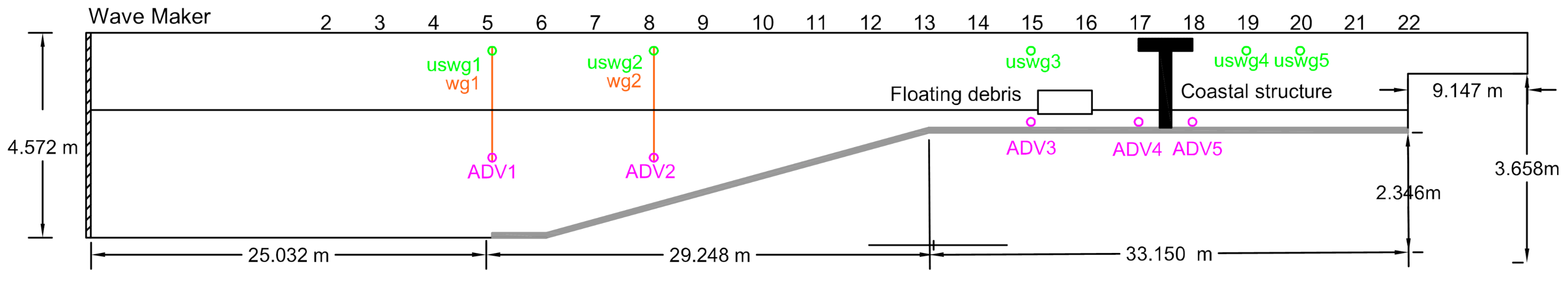
3. Experimental Work

The experimental study described in Ko and Cox [65], and Ko [37] was adopted for benchmarking the numerical SPH-FE modeling approach. These experiments had been conducted in the Large Wave Flume (LWF) at O.H. Hinsdale Wave Research Laboratory (HWRL) at Oregon State University. The flume is 104.24 m in length, 3.66 m in width, and 4.57 m in depth, and is shown in Figure 1. The LWF is equipped with a piston-type dry-back wavemaker that has a 4 m maximum hydraulic stroke actuator and a maximum speed of 4 m/s, which can generate both regular and random waves, as well as solitary waves, to simulate hurricane and tsunami waves. The LWF has adjustable bathymetry made of 20 square configurable concrete slabs. The flume includes a series of bolted holes with vertical patterns every 3.66 m along the flume for supporting test specimens, as well as, the concrete bathymetry slabs.

The coastal structure was represented by a column assembly located between bays 17 and 18, and was equipped with a load cell to measure the debris impact force. An aluminum 1:5 scale model of the standard intermodal container was used as the debris specimen. Given the fact that a standard container has dimensions of 6.1 m in length, 2.44 m in width, and 2.9 m in height, at 1:5 scale, the model had dimensions of 1.22 m × 0.49 m × 0.58 m, while the draft of the empty container was 9.1 cm. The longitudinal orientation is defined so that the major axis of the debris is parallel to the x axis and the direction of tsunami propagation. The debris specimen is located 3.5 m away from the column in the x direction. In order to control the movement of the debris and maintain the debris’ orientation, guide wires had been installed in the LWF between bays 15 and 18. The debris specimen was allowed to move freely in the x and z directions, i.e., horizontal and vertical directions, but it was restrained in the y direction, which means that there was no translation across the flume width and no yaw.

To measure the free-surface time history and fluid velocity in the x direction, several resistance and ultrasonic wave gages, and acoustic doppler velocimeter (ADV) had been installed along the flume. The error function method proposed by Thomas and Cox [77] was used to generate the wave paddle displacement in the aforementioned experiments. To maximize the volume and duration of the tsunami inundation process, the full 4 m stroke of the wave maker had been used. The time for the wave paddle to travel the full 4 m stroke, i.e., error function period, is denoted as T_erf.

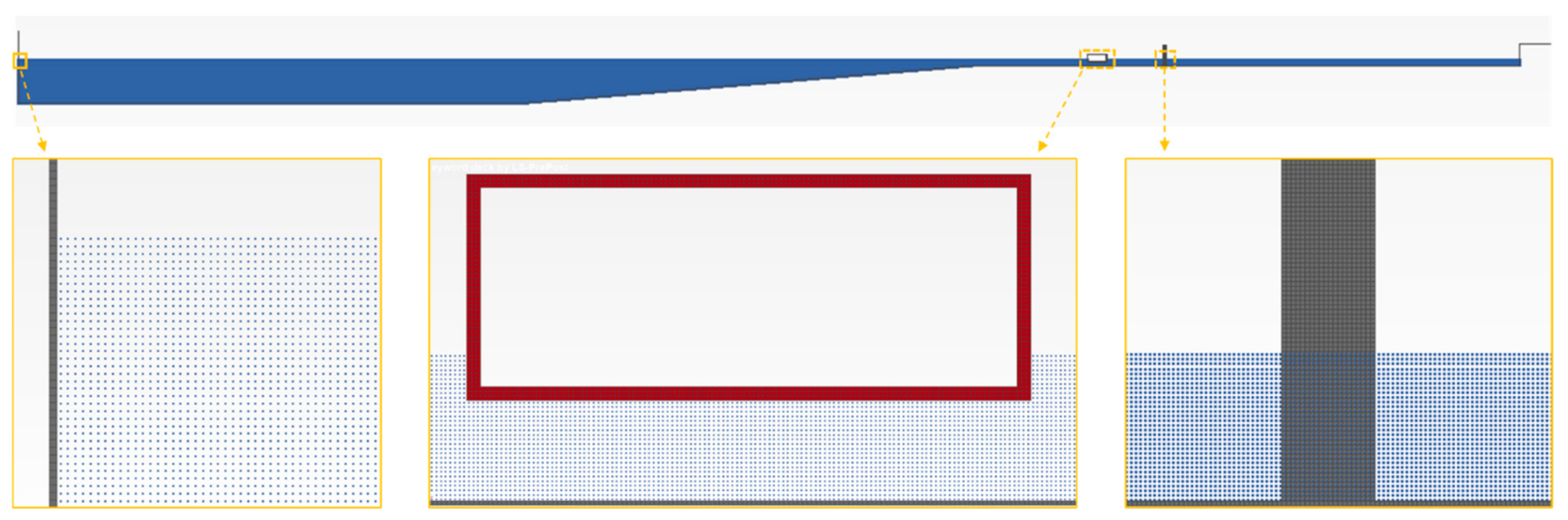
4. Coupled SPH–FEM Modeling

4.1. Numerical Settings

A numerical model of the experimental setup was developed using particles (SPH) for the fluid, and finite elements (FEM) for the flume walls, the debris specimen and the column. The bathymetry and experimental setup shown in Figure 1 was simulated via a two-dimensional model that represented a slice crossing through the mid-width of the flume, and cutting the debris and the column in two equal halves. This assumption was possible due to the debris restraints used in the experiments, which eliminated the movement of the debris across the flume width (normal to the tsunami flow). In this model, the wavemaker was represented with rigid shell elements with a prescribed horizontal motion equal to the input wavemaker displacements of the experiments found in Ko and Cox [65].

The influence of different SPH particle sizes on the computational time and numerical results was investigated by comparing sizes of 1, 2 and 3 cm, as shown in Appendix A. Decreasing the initial particle size improves the accuracy of the numerical results; however, too small sizes could cause numerical instability [78]. Considering the computational time, numerical accuracy, and calculation efficiency, the particle size of 1 cm was selected in the final numerical models presented herein. The debris and the column were generated using shell elements that had the same size with the fluid particles (1 cm), as shown in Figure 2. The final 2D numerical model consisted of 14,571 shell elements and 1,193,075 SPH particles. Given the fact that no significant deformations of the debris were observed in the selected experimental results [65] during the debris–flow interaction and impact on the structure, the debris was simulated as a rigid body. In the case of a ‘rigid’ assumption the properties of the rigid shell elements are not considered in the calculation of the time step of the explicit analyses, meaning that the time step is determined only by the remaining elements and particles. This in turn allows the explicit solver to use a significantly larger time step and reduce the required computational time per analysis.

Given the 2D nature of the numerical model, several additional calculations and assumptions had to be made in order to ensure compatibility with the actual experiments. First, the 2D geometries of the container and the column were simulated (see Figure 2). However, since the sides of the container were not simulated in the 2D model, its thickness and density were adjusted in order to simultaneously satisfy the required draft of 9.1 cm and exhibit a rotational inertia that was equivalent to the one of the experimental specimen. Then, by assuming that the ratio of the debris’ mass to the column’s mass is identical in both the numerical and experimental models, the density of the column was determined accordingly. With the beneficial effect of the ‘rigid’ assumption in mind (in terms of computational time), and the expected small effect of the steel column deformation on the overall phenomenon (e.g., fluid flow around the column and the debris–fluid–column interaction), the column was assumed to be rigid as well. Despite this assumption, since the objective of this paper was to investigate the accuracy of predicting the impact forces, the contact stiffness was reasonably calculated by the solver via the bulk modulus (defined at the material level) and Equation (18) to avoid artificially high numerical spikes generated by a rigid-to-rigid body contact.

Key parts in the development of the numerical models included the definitions of the SPH–FEM and FEM–FEM contacts interfaces. In fact, different contact algorithms were employed to define the interaction (i) between the fluid (SPH) and the flume wall, the wavemaker and the debris specimen (FE), and (ii) between the debris and the column. The interaction between the FE and the SPH particles was defined in the numerical simulation via the *CONTACT_2D_NODES_TO_SOLID contact card, with the master-slave penalty algorithm, in which the shell elements were assigned the role of the master part and the SPH particles the slave part. Moreover, the contact between the floating debris and the column was determined via the *2D_AUTOMATIC_SURFACE_TO_ SURFACE contact type, which is a segment-based two-way contact. Such segment-based contacts are preferred over node-based contacts, since the penetration can be easily traced even if it happens at locations far from existing nodal locations, and consequently tend to be more accurate but computationally more expensive. It must be noted that the contact between the fluid and the column was not simulated in the 2D model because it would generate a reflection of the bore when it reached the structure, which is not realistic given the fact that in the actual experiments the bore can escape from the sides of the column.

Despite the speed-up of the numerical analyses due to the aforementioned assumptions, it was not feasible to run the 2D model on a regular desktop and therefore all the computational analyses were run on the high-performance computing (HPC) cluster at the University of Nevada, Reno, using up to 80 cores per analysis. The analysis time ranged between 15 and 21 h depending on the hydrodynamic characteristics (i.e., water depth), which affected the total number of SPH particles.

4.2. Accuracy of Numerical Modeling

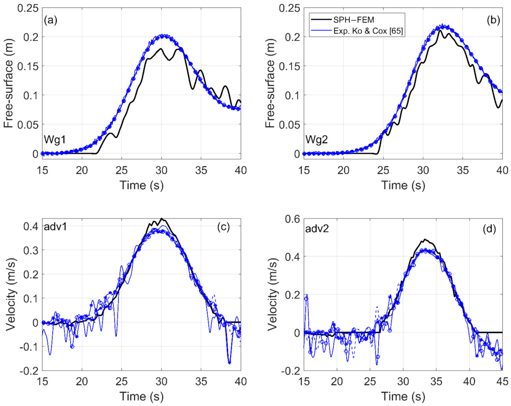
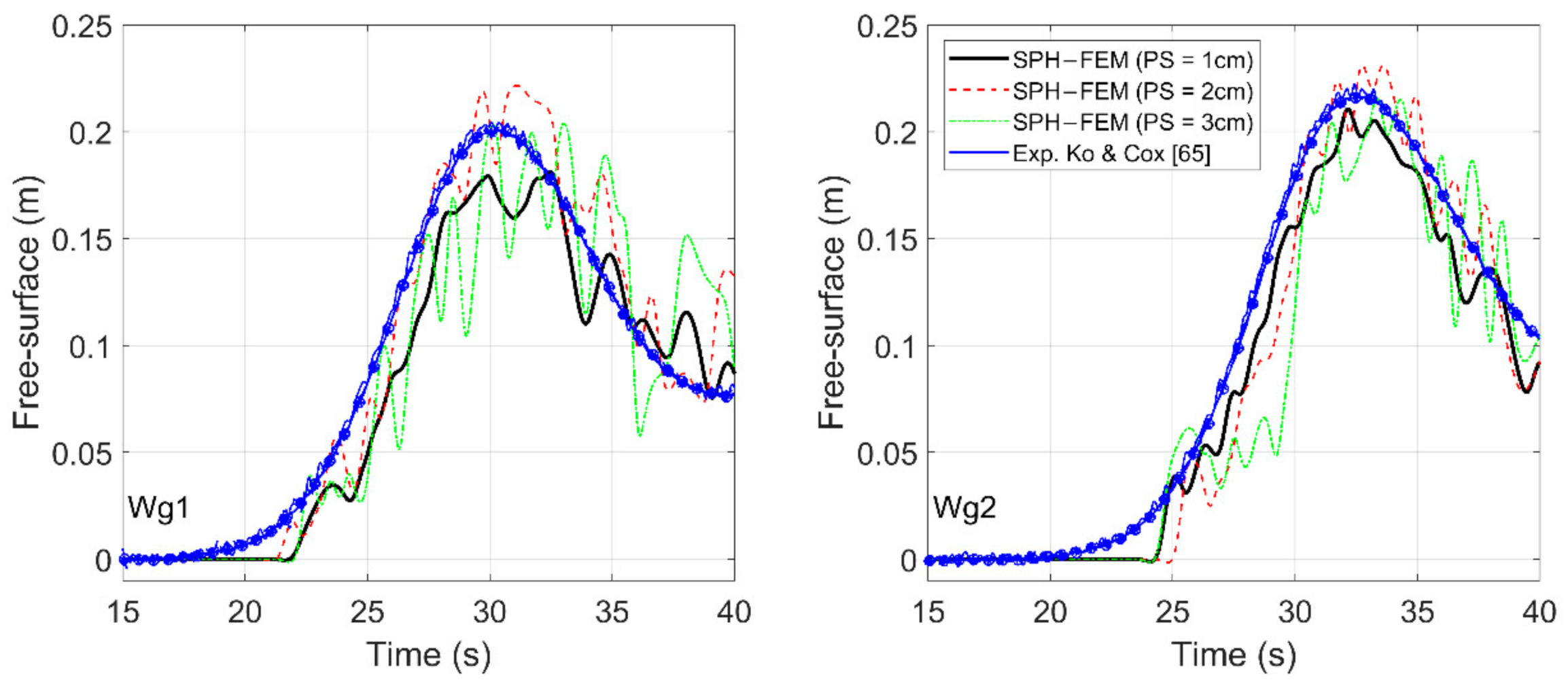
4.2.1. Free Surface and Fluid Velocities

In order to quantify the accuracy of the numerical model, the results of the free-surface and fluid velocity histories at two different distances from the wavemaker, were compared with those measured in Ko and Cox [65]. Wave gage 1 (wg1) and adv1 are the closest to the wavemaker and are located at the end of the first horizontal part, with x = 24.930 m for both instruments and z = 1.240 m for the adv. In addition to this location where the wave has propagated only over a horizontal slab, the numerical results are also compared with the experimental results at x = 35.890 m (see wg2 and adv2), which is located along the sloped part. The z coordinate of adv2 is 1.236 m. Figure 3 shows the variation of the free-surface at (a) wg1 and (b) wg2, and the fluid velocity at (c) adv1 and (d) adv2 for all trials of the experimental tests with parameters of h₁ = 2.496 m and h₂ = 0.13 m, and T_erf = 30 s from [65], where h₁ and h₂ corresponds to the initial water depth offshore (at wavemaker location) and on the coast close to the debris, respectively. It can be observed that both the free-surface and fluid velocity histories computed by the numerical model are in good agreement with the experimental data, both in terms of the peak values and temporal evolution. There are some underpredictions of the maximum wave height and some overpredictions of the velocity but those do not exceed 6% for the selected wave. In addition to this good agreement, the encouraging thing is that the numerical model can predict the relative increase between wg2 and wg1 of the maximum free surface, indicating that the SPH–FEM coupled approach can capture the interaction of the fluid with the sloped part of the flume and result in a similar non-linear transformation of the wave during the shoaling process.

Figure 4 shows a comparison of the numerically predicted maximum values of the free surface at the locations (a) wg1 and (b) wg2 with the experimental data for all the tested tsunami waves (T_erf = 30 s, 40 s, 45 s) for h₁ = 2.496 m and h₂ = 0.13 m. Promising agreement with the experimental was achieved, with the maximum deviation from the average value of the measured data at wg1 being 6.3%, 11.7%, and 13.7% for T_erf = 30, 40 and 45 s, respectively. At wg2, the maximum differences are 4%, 15.9%, and 15.2%. As expected, both the numerical and experimental data show that the shorter T_erf, i.e., T_erf = 30 s gives greater inundation depths at the two locations. This also seems to be true for the peak velocities, especially those measured at adv2, as shown in Figure 5. The latter figure presents the experimentally and numerically recorded maximum velocities at (a) adv 1 and (b) adv2 for the same hydrodynamic conditions as in Figure 4 (h₁ = 2.496 m). Similarly to the free surfaces, the SPH–FEM approach can predict reasonably the maximum fluid velocities with maximum deviations of 3%, 4.7%, and 2% at adv1 for the three different tsunami bores (T_erf = 30, 40, and 45 s), respectively. At adv2, the maximum differences are 6%, 14%, and 22%, respectively. It is noteworthy that (i) the experimentally recorded peak fluid velocities in Ko and Cox [65] had significantly larger variability than the measurements of the free surface, and (ii) the most sensitive experimental results corresponded to the measured velocities of the slower flows (e.g., for T_erf = 45 s), for which the numerical modeling yielded the largest deviations (underprediction of approximately 25%).

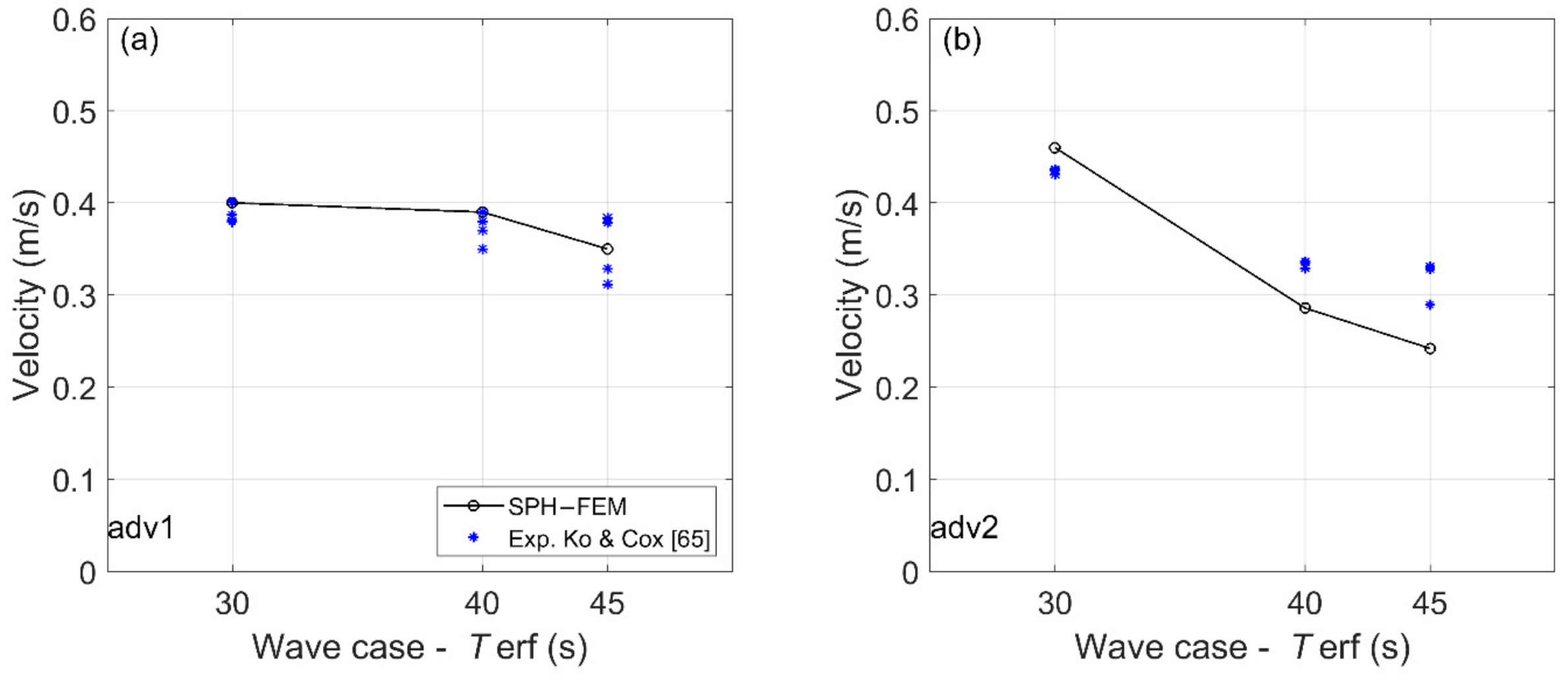
4.2.2. Debris Motion

Although the reasonable predictions of the free surface and fluid velocities achieved by the numerical simulations increase the confidence in the SPH solver and the coupled SPH–FEM approach, one of the most critical aspect for future risk assessment studies is the ability to estimate the debris transport and propagation overland. To this end, Figure 6 shows the velocity history of the debris specimen for one of the hydrodynamic conditions with h₂ = 0.13 m and T_erf = 30 s. The debris velocity was generated based on the publicly available videos on DesignSafe (i.e., Ko and Cox [65]), using a color-based tracking algorithm. However, it must be noted that the estimated velocities (from the videos of the experiments) could potentially entail some errors due to the fact that the ceiling cameras could not be perpendicular to the top surface of the debris for the whole propagation process (from its initial position up to the coastal structure). A more accurate estimate would require a perspective correction, as in Ko [37], which was not done herein due to the lack of adequate information.

Since the debris specimen was modeled as a solid body, in order to evaluate the accuracy of the debris velocity from the SPH–FEM simulation, the velocity was output at four nodes of the debris, which corresponded to the external corners. Figure 6 presents the nodal velocities at the lower right and left corner together with the experimental velocity and a reasonable agreement is observed. The numerical and experimental simulations seem to give similar debris velocities when the bore reaches the container and starts transporting it. However, as the debris propagation continues, the numerical model seems to accelerate more and reach a larger velocity than the experimental specimen before the impact on the column. This in turn causes the numerical model of the container to cross the 3.5 m (initial distance between debris-column) faster and impact the column earlier than the experiment.

One of the possible explanations for the observed differences lies in the 2D formulation of the current numerical model, which implies that the pressures applied from the bore on the offshore face of the debris (i.e., the mechanism causing the debris movement) are uniform across the debris width. However, in the actual experiments the pressures on the offshore face of the debris (and below its bottom side) are expected to be smaller at locations close to the sidewalls than the mid-width due to 3D effects. In other words, some of the bore pressures on the debris are relieved close to the vertical sides of the debris since the bore can propagate along these sides, given that there is a large area between the flume walls and the debris. Moreover, it must be clarified than in the presented numerical results the debris was restrained to move only in the horizontal direction, i.e., the direction of the bore propagation, eliminating any pitching that could potentially attenuate the debris transport.

The decision to restrain the debris was made based on the findings of Ko [37], who stated that there was significant variability in the experimentally recorded impact forces due to: (i) the “off-centered” impact of the debris on the load cell, and (ii) the effect of the pitch angle that was present in some trials but not in others. For example, it can be estimated from the figures of Ko and Cox [65] that for a debris velocity of approximately 1.4–1.5 m/s the “off-centered” impact can give maximum impact forces that are reduced by approximately 40% relative to the centered case. This explains why in the aforementioned study was decided to consider only the centered experimental results, and why in the present numerical investigation the debris was not allowed to pitch during the validation phase.

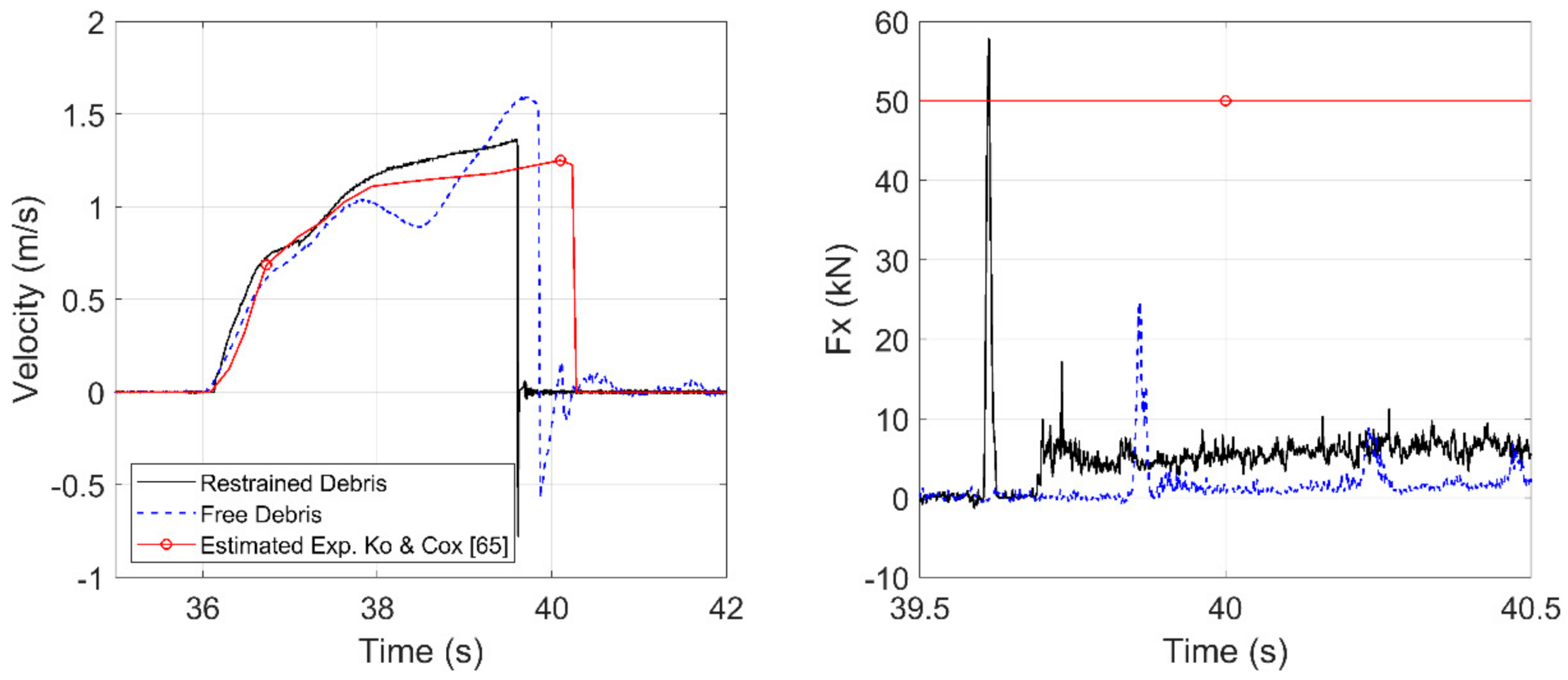
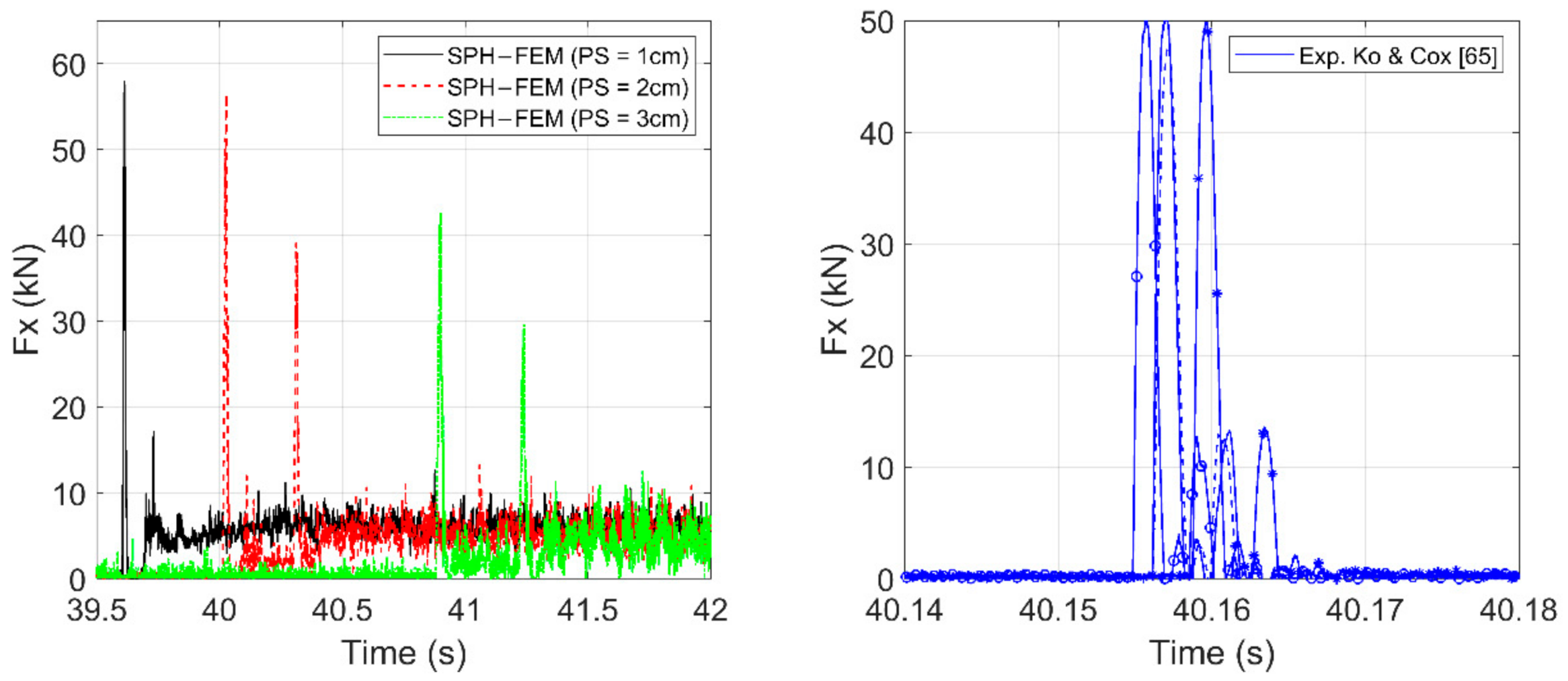
4.2.3. Debris Impact Force

Figure 7 shows the time histories of the debris impact forces on the column for two selected hydrodynamic conditions, with T_erf = 30 s and T_erf = 45 s for the same initial water depth h₂ = 0.13 m. Subfigures (a) and (b) correspond to T_erf = 30 s for the numerical and experimental data respectively, and subfigures (c) and (d) show the same results but for T_erf = 45 s.The agreement between the computations and the different trials of the physical tests is reasonable, both in terms of the peak impact force and in the overall trends. For instance, for the case of T_erf = 30 s, the SPH–FEM models predict a relatively higher impact force than the experiments by approximately 15%. However, this can be explained by the fact that as shown in Figure 6 the numerically predicted impact velocity was approximately 20% higher than the experimental one. Given the fact that the majority of the available simplified equations for debris impact loads, such as those presented in FEMA P646 [3] and ASCE [79], are a linear function of the impact velocity, it is reasonable to obtain larger impact forces from the numerical simulations since they predict larger velocities. Apart from the similarities in the results, there are also two noticeable differences:

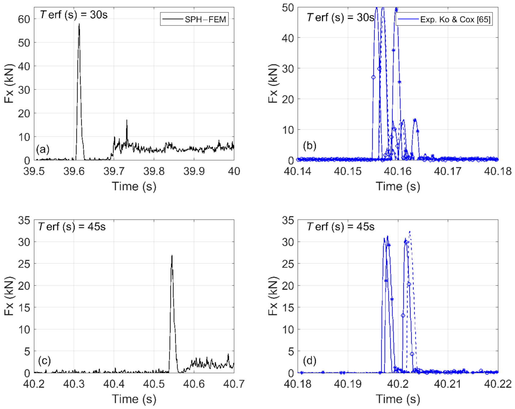
• In the numerical simulations, the impact force on the column is applied earlier for T_erf = 30 s and later for T_erf = 45 s compared to the physical tests. However, these differences in the instants could be justified by the differences in the debris velocities, which were most likely overpredicted and underpredicted, respectively, as indicated by the trends in the maximum values. In other words, it is reasonable for the debris impact to occur earlier when the numerical models overpredict the magnitude of the impact, because the reason is the larger debris velocity.
• Immediately after the primary impact force, the column in the physical tests experienced a second short-duration impact force, which is relatively small compared to the main impact. However, this trend was not observed in the numerical results. In contrast, the simulations show a long duration load after the initial impact, which seems to have a nearly constant magnitude. This difference can be attributed again to the 2D simplification made in the numerical models, which are unable to allow the fluid to escape from the sides of the debris after the initial impact on the column and relieve the pressures applied on its offshore face. This leads consequently to the stagnation of the flow in front of the offshore face, resulting in a nearly steady-state horizontal damming load.

The trends of the peak values of the impact forces observed in the previous figure are also verified in Figure 8, which plots the corresponding maximum values from the experiments and the computational models for all three hydrodynamic flows (T_erf = 30, 40, and 45 s) with h₁ = 2.496 m and h₂ = 0.13 m. In fact, this figure reveals that the maximum deviation from the measured values is 14%, 25%, and 19% for the three flows, respectively, which is promising given the differences in the debris velocities. Moreover, another observation that reinforces the confidence in the SPH–FEM modeling approach is that it presents similar trends with the physical tests (as a function of T_erf,) since both of them give larger debris velocities and impact forces for the smallest T_erf = 30 s representing the more transient flow with the largest fluid velocities.

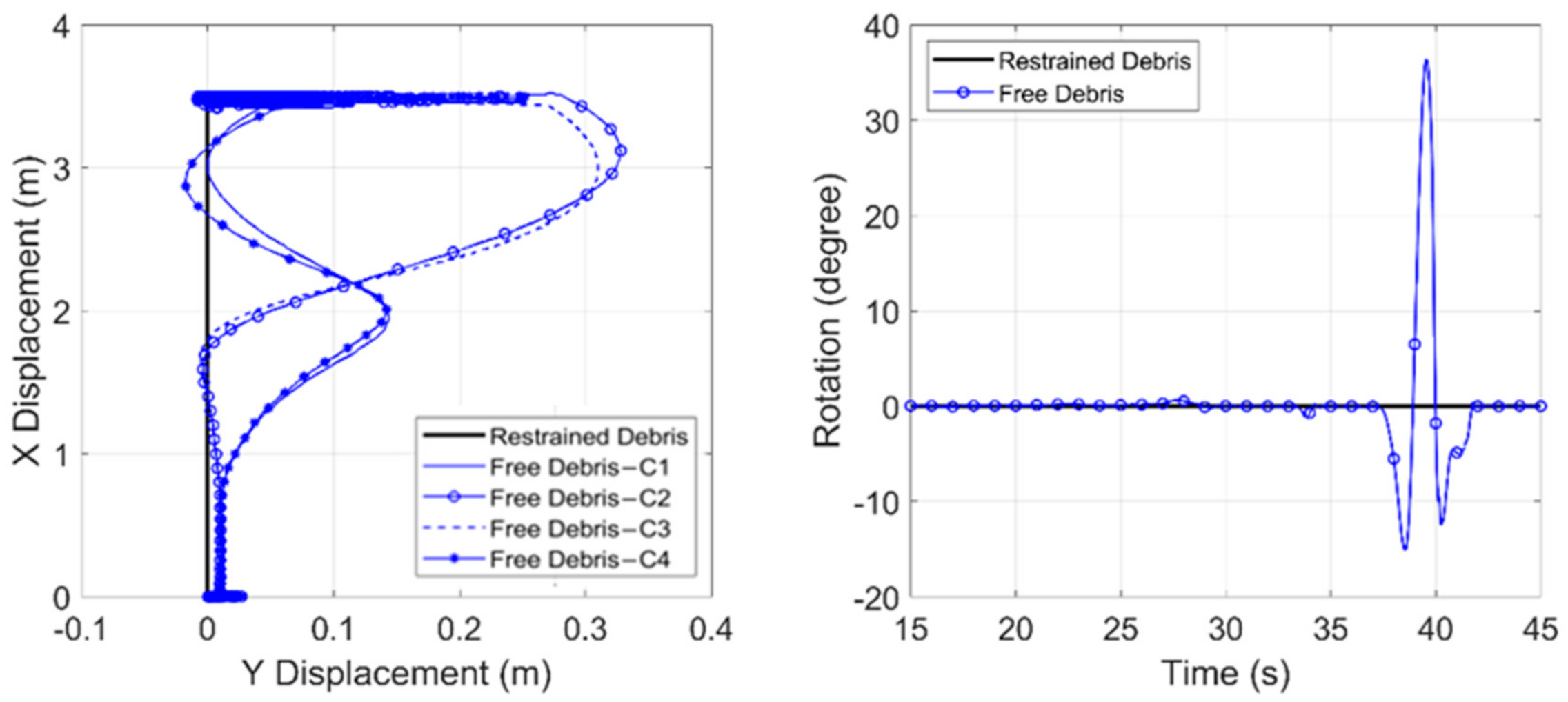
5. Role of Debris Restraints

Given the fact that in the validation section the debris was restrained in order to make it more consistent with the experiments, it is essential to assess the role of the restraint for the debris–wave interaction, the debris transport overland and the impact on the structure. To this end, the restrained model of the previous section was compared with another model that allowed the debris to move freely in the 2D plane (horizontal and vertical displacement, and pitching). Figure 9 presents several selected snapshots of the tsunami flow with T_erf = 30 s for h₂ = 0.13 m as the free debris propagates towards the column location, from the instant that the bore starts moving the debris up to the instant of the second impact. Among these snapshots, ‘e’, ‘f’, ‘g’ correspond to following instants: (i) slightly before the first impact on the column, (ii) after the 1st impact, and (iii) at the instant of the 2nd impact on the column, respectively. As shown, the debris starts pitching in the clockwise direction up to the point that the onshore bottom corner tends to touch the bottom of the flume, after which it immediately changes the direction of pitching. It is also revealed that the large counter-clockwise pitching continues until the debris reaches the column location, which results in a non-normal impact angle and a consequently non-uniform contact of the onshore vertical face of the debris with the column, affecting the contact area and consequently the maximum impact forces. After the initial impact, the debris bounces back and re-impacts the column with a clockwise pitching angle, which generates a smaller magnitude impulse.

Figure 10 presents a quantitative comparison between the debris motion of the two cases. In the case of the free debris four locations are selected for presentation, including, the lower left corner (C1), the lower right corner (C2), the upper right corner (C3), and the upper left corner (C4). The x-displacement vs. y displacement curves for the free movement debris reveals that the two lower corners move in the opposite y direction as the debris moves along the x direction. A similar motion trend is observed for the two upper corners as well. The opposite movement in the y direction indicates the initiation of the debris rotation. To evaluate the level of the pitching, the rotation angle of the debris is calculated using the corner displacements and is presented on the right subplot of Figure 10. Based on this figure it becomes evident that the debris starts rotating clockwise after the bore reaches its location (negative rotation), then as it transports inland it changes the direction of rotation until it reaches the maximum rotation of approximately 37° slightly before the primary impact on the column, and then rotates in the opposite direction as it interacts with the column, until it stabilizes at a zero angle and the long duration damming process is initiated.

The debris velocity and impact forces histories for the free and restrained container models are presented in Figure 11. Interestingly, although it was expected the peak impact velocity to be affected by the pitching, the expectation was that the free debris would exhibit a more significant wave–structure interaction (due to the larger vertical displacements and rotation), which would dissipate more of the energy of the bore leading to a smaller horizontal debris velocity and a delayed arrival at the column location. While the delayed arrival did happen as expected and the debris velocity was indeed smaller than the respective velocity of the restrained model, this was true only at some instants during the debris transport inland and not at the instant of the impact on the column. The impact velocity of the free debris was surprisingly larger than the restrained one, which highlights the complexity and non-linearity of the debris interaction with the turbulent flow.

Another interesting finding can be reached from the subplot of the impact forces, according to which, the column experiences a significantly larger impact force from the restrained debris than the free case, although the latter one impacts the column with a larger velocity. The debris restraint seems to increase the maximum impact force by approximately a factor of 2.3 relative to the free case and reach the experimentally recorded values. The above trend could be attributed to the presence of debris pitching that affects the impact angle on the column, since as was observed in the swinging in-air tests of Ko [37] the cases with a zero pitch angle tended to give larger impact forces than the larger pitch angles, even when the debris impact velocities were the same.

The above finding indicates that future predictive equations might have to be a function of not only the impact velocity but also the impact angle, while design methodologies and risk assessment frameworks should be able to predict these two parameters. Ideally, the location of the impact on the coastal structure should also be estimated since the structural damage caused by the container could be very localized (close to the point of contact) if the debris impacts a coastal structure with a non-normal pitching angle.

6. Effect of Hydraulic Conditions on Debris Motion and Impact Forces

6.1. Tsunami Flow Characteristics

To gain further insight into the debris–flow interaction and impact on coastal structures, this section will evaluate the effects of the flow characteristics by considering the three different cases with T_erf = 30 s, T_erf = 40 s, and T_erf = 45 s for h₁ = 2.496 m and h₂ = 0.13 m tested in [37]. In this section, the debris will be considered free in the 2D plane since it is considered more realistic, despite the fact that the restrained model captured better the experimental data. Comparison of the free surface and fluid velocity at a location close to the container, i.e., x = 62 m, is depicted in Figure 12. As discussed in [37], the error function (T_erf) affects the wave characteristics, and particularly the wave height and fluid velocity. The new figure shows that although there are similarities in the free-surface histories for all three waves, the smallest T_erf (which corresponds to the faster movement of the wavemaker) exhibits the largest peak values for the free surface and the fluid velocity, with the most noticeable differences observed in the fluid velocities. Interestingly, as the T_erf increases the flow height and fluid velocity is reducing, while the duration of the inundation is elongated, which indicates that the flow is switching from a highly transient bore to a more steady-state flow.

Figure 13 presents two selected snapshots of the debris–fluid interaction as the container propagates inland for two selected tsunami waves with T_erf = 30 s, and T_erf = 45 s, respectively. While both waves present similar trends in the debris motion, which comprises of a clockwise rotation followed by a counter-clockwise one, the faster moving bore results in larger particle velocities around the debris that in turn cause larger pitching of the container. This would indicate that the pitching of the debris is mainly caused by the larger velocities, and not that much by the differences in the free surface, which are much smaller. Figure 14 plots the vertical movement of the lower-right corner of the container and its rotation throughout the propagation inland. This figure illustrates that the debris flow is indeed highly dependent on the tsunami characteristics and that the fastest bore (T_erf = 30 s) can cause pitching angles that are approximately 85% larger than those of the slowest wave (T_erf = 45 s). This larger rotation leads to an increase in the upward vertical movement of the offshore face of the container, which enables it to impact structural locations at higher elevations.

Combining the trends of the previous figures and snapshots, it is possible to identify three characteristic time instants in the motion of the debris for the case of T_erf = 30 s, as shown below:

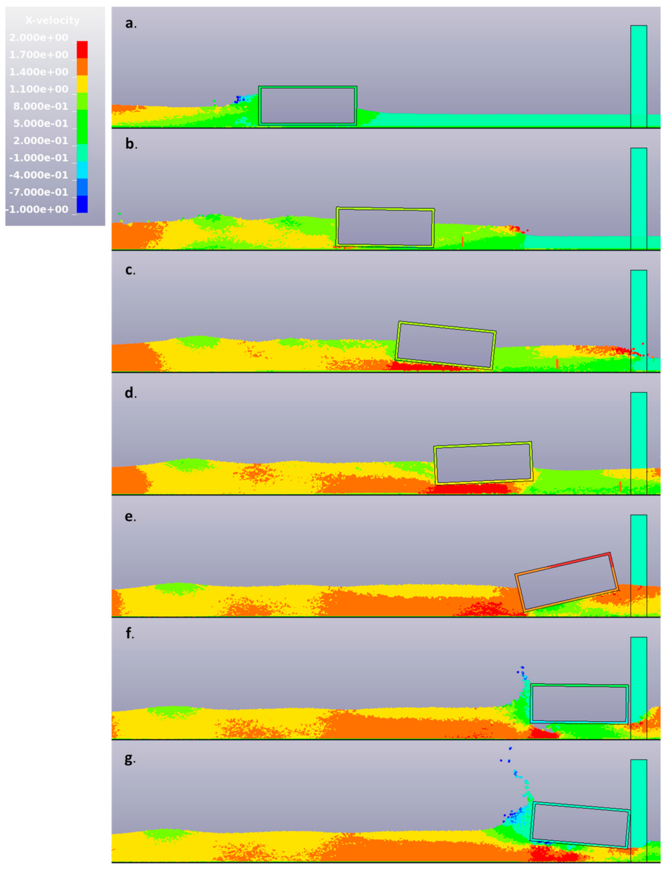
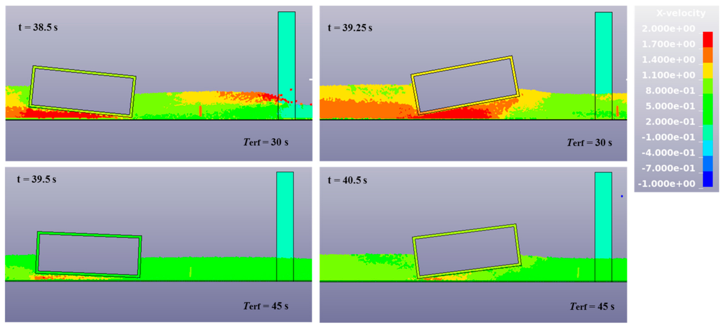
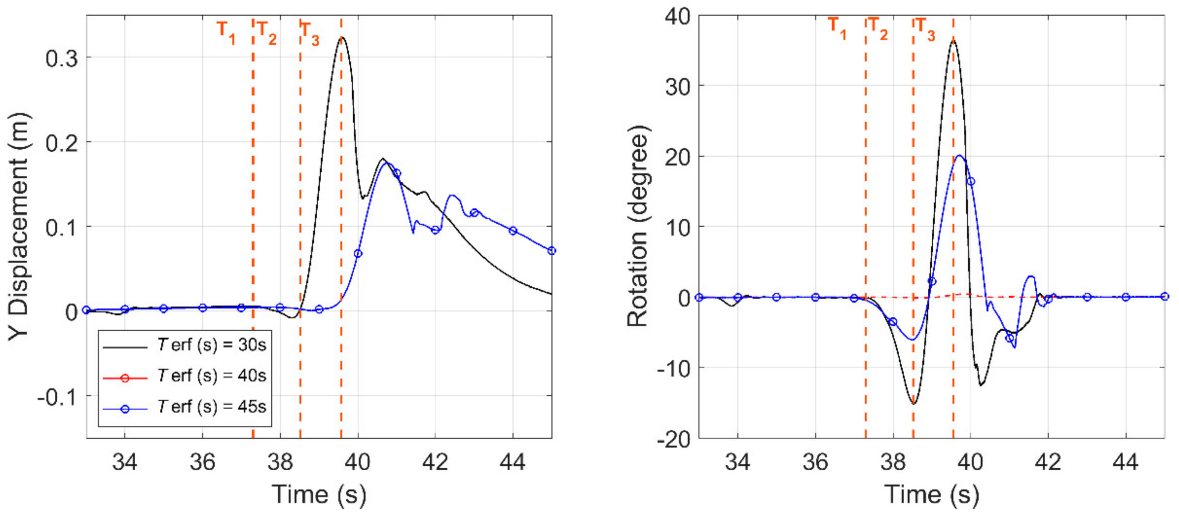
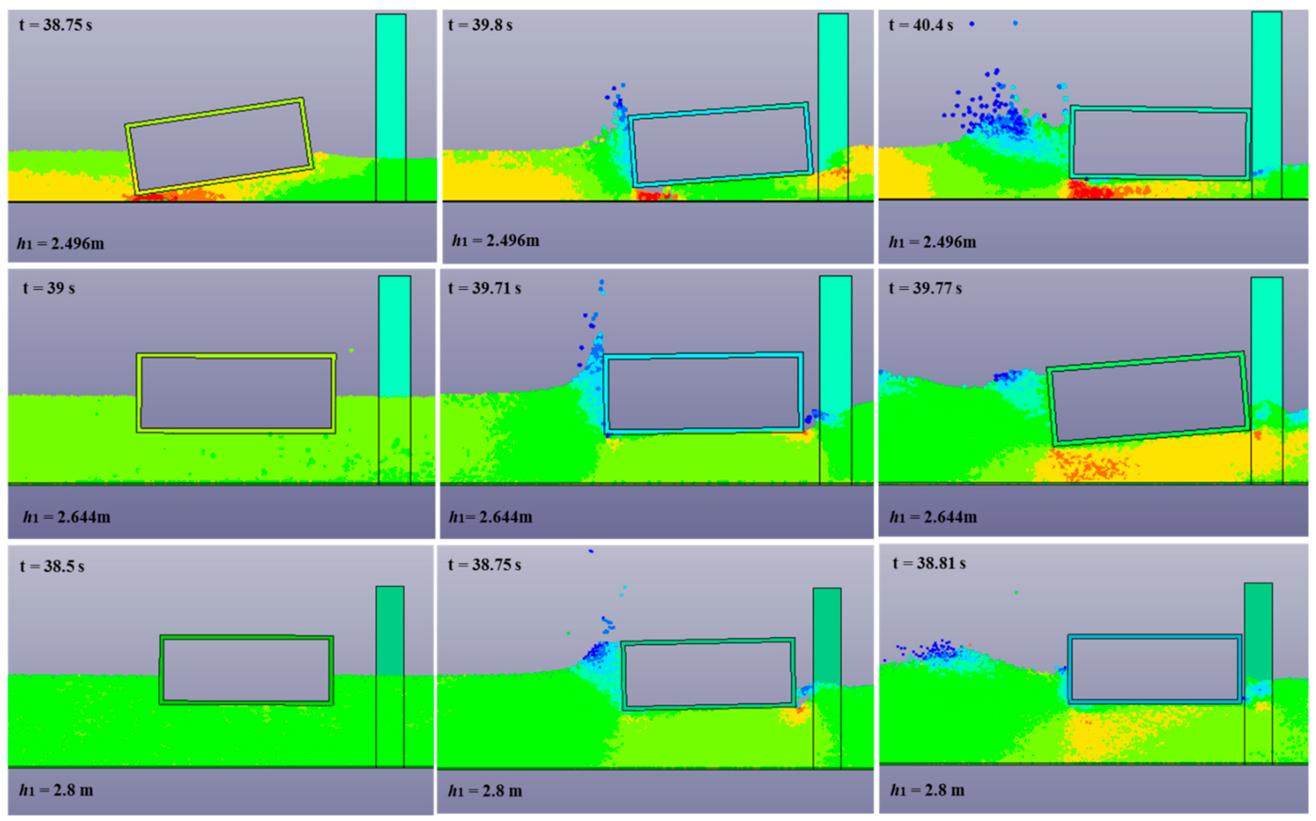
• T1: This time instant represents the initiation of the debris rotation. It occurs slightly after the tsunami has started pushing the debris inland. After that initial contact with the bore, the debris starts accelerating and as the flow below the debris increases and the bore front surpasses the debris, the latter one starts rotating clockwise (see also snapshots b. and c. in Figure 10).
• T2: This instant corresponds to the largest clockwise rotation, at which point the lower right (onshore) corner has displaced downward so much that it impacts the floor of the flume. When this impact takes place, a restoring force is applied to the debris causing it to start rotating in the opposite direction (counter-clockwise).
• T3: After the primary debris impact on the flume floor and the initiation of the counter-clockwise rotation, the debris continues rotating in this direction until it reaches the maximum pitch angle, which tends to occur slightly before the primary debris impact on the column. At this instant, it is possible for the lower left (offshore) corner of the debris to touch the floor of the flume before it impacts the column. However, this will depend on the initial relative distance between the debris and the coastal structure, as well as, the hydrodynamic conditions. This means that instant T3 represents the maximum clockwise pitching angle, which might be close to the impact angle, but not necessarily the same. Future studies should investigate different debris–structure relative distances, and a larger range of hydrodynamic conditions in order to determine the dependence of the maximum pitching angle and the impact angle on these parameters. Ideally, such studies should employ three-dimensional models, which are expected to be more accurate than two-dimensional models.

The debris impact forces on the column, including both time histories and the peak value versus the impact velocity, are presented in Figure 15 for all the tsunami waves of h₂ = 0.13 m. As expected, larger tsunami waves have more energy and higher particle velocities, which lead to higher values of the debris impact velocities and impulsive forces on the column. This is why the wave with T_erf = 30 s exerts the largest impact force on the column. Interestingly, the largest/fastest tsunami bores also result in higher damming loads, with T_erf = 30 s giving almost 3-fold larger values than T_erf = 45 s. However, this observation must be taken with caution, since, as explained earlier, the 2D nature of the numerical models can lead to over-prediction of the damming loads. Last but not least, the right subplot of Figure 15 reveals that contrary to the existing simplified equations of debris loads (e.g., FEMA P626 [3]), the impact forces might not necessarily be a linear function of the impact velocity, at least for the specific hydrodynamic conditions. In fact, when the debris velocity increases above a certain limit (e.g., 1.1 m/s for this water depth) the rate of the increase in the impact force with the velocity decreases, resulting in a non-linear increase in the force. This behavior can be explained by the trends observed in the previous figures, according to which, the largest impact velocity corresponds to the fastest bore (T_erf = 30 s) that cause significant pitching of the debris and non-normal impact on the column. Ultimately, the results presented herein indicate that the debris impact forces might be a function of both the debris velocity and pitching angle at the instant of the impact on the coastal structure. However, this indication must be further verified with validated three-dimensional models. Ideally, such future models should simulate the debris and the coastal structure as flexible bodies, since that will enable a more realistic prediction of the impact duration and determine its dependence on the debris velocity and pitch angle.

The above findings seem to extend and complement the findings of previous studies, which have demonstrated the critical role of the relative tsunami–structure or debris–structure angle, in the estimation of hydrodynamic and debris loads, respectively. For example, Istrati and Buckle [44,80] demonstrated the dependence of the maximum tsunami loads on the skew angle of a bridge and the angle of attack (obliqueness of the wave), respectively, while Haehnel and Daly [36] and Derschum et al. [40] revealed experimentally the dependence of the debris loads on the yaw angle of the impact on the structure, for wooden logs and shipping containers, respectively. The former research study proposed a reduction coefficient for cases of oblique debris impact on a structure, and was later on the basis for the development of the orientation coefficient (equal to 0.65) in the Tsunami chapter of ASCE 7-16 [79]. Interestingly, the debris rotation and oblique collisions between adjacent containers were suggested as a critical factor in Stolle et al. [81], since these could result in energy losses and consequently reduce the impact forces on coastal structures. The latter authors simplified the estimation of the impact loads induced by multiple debris, by assuming them to be a function of an area coefficient that accounted for the impact debris geometry and compactness. However, they noted that accounting for the impact angle of the agglomeration in future studies, would be physically more realistic. Last but not least, the experimental observations of Shafiei et al. [38] are perhaps the closest in agreement with the findings of the current study, since they observed that the debris always impacted the vertical structure at non-zero pitching angle, which ranged between 3 and 10° and 15 and 30° for a rigid rectangular box and a disc, respectively. This pitching angle had a major effect because it governed the variability of the impact accelerations and caused a large vertical load (in the case of a horizontal tsunami flow) that was approximately 60% of the horizontal one.

6.2. Initial Water Depth

In addition to the effect of the tsunami characteristics, it is of interest to evaluate the effect of the initial water depth on the debris motion, and the debris interaction with the column and the bottom of the flume. For this purpose, two of the water depths tested in Ko [37], i.e., h₁ = 2.496 and 2.664 m and a new depth with h₁ = 2.8 m were considered for a range of tsunami flows. These offshore water depths translated into local initial water depths of 0.13, 0.30 and 0.43 m, respectively, at the debris location. Figure 16 illustrates (a) the variation of the free surface, (b) thefluid velocity, (c) the debris vertical displacement, (d) the debris rotation, (e) the debris velocity and (f) the impact force. The free-surface histories are plotted close to the offshore side of the debris, at x = 62 m, and are calculated relative to the initial water level, while the fluid velocities are plotted at the same x coordinate at the level of the initial free surface (i.e., 9.1 cm above the bottom of the debris). This means that the absolute elevation of the locations at which the fluid velocities are plotted are different for each water depth, but the relative distance from the bottom of the debris is the same. The figure reveals small differences in the maximum bore heights and nearly negligible differences in the fluid velocity histories close to the debris location, for three water depths. There are some differences in the free-surface history of the shallower water level relative to the two larger depths, with the most obvious difference in the bore front and the instant of the arrival at x = 62 m. In the case of the deeper water, the tsunami waves are arriving slightly faster, which is attributable to the increase in the wave celerity offshore caused by the increase in the water depth. Nonetheless, the tsunami bores at the debris location are similar enough for the three water depths, enabling the proper investigation of the effect of this parameter.

Interestingly, despite the smaller bore height in the case of the h₁ = 2.496 m relative to the other depths, this case exhibits the largest vertical displacement of the debris (at its onshore corner) and the largest pitching. In fact, the maximum pitching angle seems to consistently decrease with the increase in the water depth, with the shallowest case inducing an approximately 5-fold larger maximum pitching angle relative to the deepest case of 2.8 m. This demonstrates that the rotation of the debris is highly dependent on the initial water depth. Moreover, in addition to the differences in the magnitudes, it can be observed that the previously identified pattern in the debris motion, which involved an initial clockwise debris rotation followed by a counter-clockwise one before the impact on the column, is not consistent for all the water depths. For larger initial depths it is possible to notice an opposite sequence of debris rotations (i.e., for h₁ = 2.66 m) or just a clockwise rotation before the initial debris contact with the column (i.e., for h₁ = 2.8 m). Last but not least, in contrast to the differences in the vertical displacement and rotation of the debris, the debris horizontal velocities present more similarities. The major difference is observed in the fact that the deeper cases exhibit a gradual increase in the debris velocity, which becomes nearly constant as it approaches the coastal structure, while in the shallowest case more abrupt increases in the debris velocity are observed that result in a larger impact velocity on the column. Despite the larger debris impact velocity for h₁ = 2.496 m (for the specific tsunami bore), this case gives similar impact forces with the large water depths, which can be justified by the higher level of pitching in the former case.

Figure 17 presents selected snapshots for the three water depths and T_erf = 40 s, as the debris moves inland and impacts the coastal structure. This visual representation of the phenomenon verifies the previously observed trends, with the two larger water depths being associated with nearly a consistent debris orientation (small rotation) contrary to the shallow water that is dominated by debris pitching effects. Moreover, despite the similar bore velocities at x = 62 m (a few meters from the debris) observed in Figure 16, the fringe plots of the fluid particle velocities reveal that there are significant differences in the flow around the debris, since in the shallow case the flow seems to accelerate more below the debris. This is probably due to the fact that in the latter case the bore is more restricted and does not have as much space to propagate below the debris as in deeper waters, resulting in faster flows horizontally that tend to uplift on one side of the debris and consequently rotate it. Another major difference lies in the fact that when the initial water level is low, the pitching of the debris can move one of its corners downwards so much that it impacts the bottom of the flume. This contact between the debris and the flume complicates further the debris–fluid interaction and is a distinguishable feature of the small water depths only. Last, but not least the snapshots reveal major differences in the fluid flow below the debris after the initial impact on the column, which affects the number of secondary impacts and their magnitude, as well as, the damming loads. For example, smaller damming loads can be noticed in the case of larger water depths, because less of the bore gets reflected on the structure and more of it propagates onshore by moving below the debris. However, these differences might be exaggerated by the 2D assumption made in the development of the numerical models.

The maximum debris impact forces as a function of the impact velocities for all the water depths and bores, are presented in Figure 18. This figure reveals, that although for larger water depths (e.g., h₁ = 2.66 and 2.8 m) the relationship between the maximum debris impact force and impact velocity is nearly linear, which agrees with existing predictive equations (e.g., FEMA P646 [3] and ASCE [79]), for small water depth the trend seems to be non-linear. In fact, in the latter case, after the exceedance of the debris velocities above a certain limit, the impact force increases less than what a linear force–velocity assumption would suggest, indicating that predictive equations that utilize such an assumption might yield conservative results. To investigate whether such an indication is true, additional parametric investigations are required, followed by direct comparisons with available simplified equations, which is beyond to scope of this manuscript. However, the results presented herein raise the question on whether future predictive equations of debris loads should: (i) be a function of the water depth, so that for large initial water depths a linear impact force–velocity relationship is used and for shallow depths a non-linear one that will account for the possibility of debris pitching and non-normal impact angle on the structure, especially if the structure is located close to the location of the debris entrainment, and (ii) limit the applicability of the linear force–velocity equations to a certain velocity limit, above which, the rate of the force increase with the velocity will drop significantly.

As explained earlier, the indications of this preliminary numerical investigation should be verified with follow-up expanded studies that will include a wider range of hydrodynamic conditions (e.g., faster flows and more water depths) and different relative distances between the debris and the coastal structure. The latter parameter is especially crucial, since as observed in Goseberg et al. [82] the debris tended to yaw towards an equilibrium position as it propagated inland, in which the long axis was perpendicular to the flow direction. It would be interesting to see if the pitching of the debris will be damped out in the case where it could propagate for a longer distance before impacting the structure. If such a behavior was true, then the significance of pitching effects documented herein might be applicable only to locations near the debris entrainment by the bore, and disappear after a certain propagation distance. Moreover, although the current 2D SPH–FEM models were validated against the restrained debris experiments of Ko [37] and Ko and Cox [65], future studies should employ 3D numerical models that will be able to simulate both the yaw and roll of the debris, in order to ensure that the influence of the pitching angle on the impact forces identified by the current study is not affected by the 2D assumption. Last but not least, given the observed complex interaction of the debris with a simplified vertical coastal structure, it would be interesting for future studies to investigate how to debris will interact with more complex structural geometries, such as elevated decks with overhangs, piloti-type buildings with columns or multiple structures in urban environments.

7. Summary and Conclusions

Given the documented catastrophic effects of large debris in past tsunamis, and the difficulty of simulating numerically such effects, this study presents a coupled SPH–FEM modeling approach and evaluates its capability to predict both the debris–fluid interaction and the impact on a coastal structure. In this modeling approach the fluid was modeled via particles, based on the weakly compressible smoothed particle hydrodynamics, while the wavemaker, flume, debris and structure were modeled with mesh-based finite elements. The interaction between the fluid and solid bodies was defined via node-to-solid contacts, while the interaction of solid bodies (e.g., debris–flume, debris–structure) was defined via a two-way segment-based contact that could trace the impact at any location of the body. For the validation of the coupled modeling, the large-scale experimental data from Ko and Cox [65] and Ko [37] were selected as a benchmark. In these experiments, a tsunami-like wave was generated offshore via a wavemaker, which then propagated over a complex bathymetry, forming a transient flow on the coast that entrained the debris and propagated it onshore until it impacted a vertical column. The fact that the debris was restrained experimentally to move only in the direction of the flow (i.e., no yaw and no movement across the flume width) enabled the development of a two-dimensional (2D) numerical model instead of a 3D one, which reduced consequently the required computational time.

The comparison between the experimental and numerical results revealed an overall acceptable accuracy of the SPH–FEM coupled modeling approach, with some parameters being estimated more accurately than other, as explained below:

• The free surface and fluid velocities had good agreement with the experimentally recorded results, both offshore and during the wave propagation along the slope. The deviation of the maximum wave height from the average value of the experimental tests ranged between 4% and 15.2%, while the deviation of the maximum fluid velocities was between 2% and 22%, depending on the location along the flume and the tsunami flow. These results showed that the numerical model can predict the relative increase in the free surface and fluid velocities as the wave propagates over the sloped part and undergoes a non-linear transformation, indicating that the fluid–flume contact worked properly.
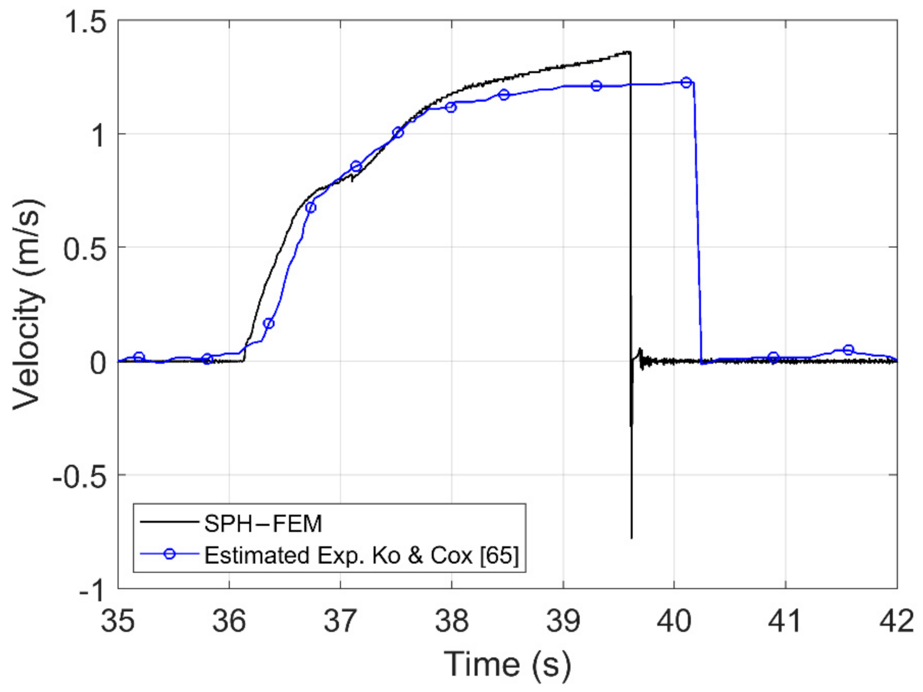
• The SPH–FEM models estimate similar debris velocities with the experiments, especially when the bore reaches the container and starts transporting it. However, as the debris propagation inland continues, the numerical model tends to accelerate more and reach an impact velocity that is approximately 20% larger than in the experiments, leading consequently to some differences in the arrival time at the column location. One possible explanation for these differences lies in the 2D formulation of the current numerical model, which implies that the pressures applied from the bore on the offshore face of the debris is uniform across the debris width, which is not necessarily the case in real 3D environments.
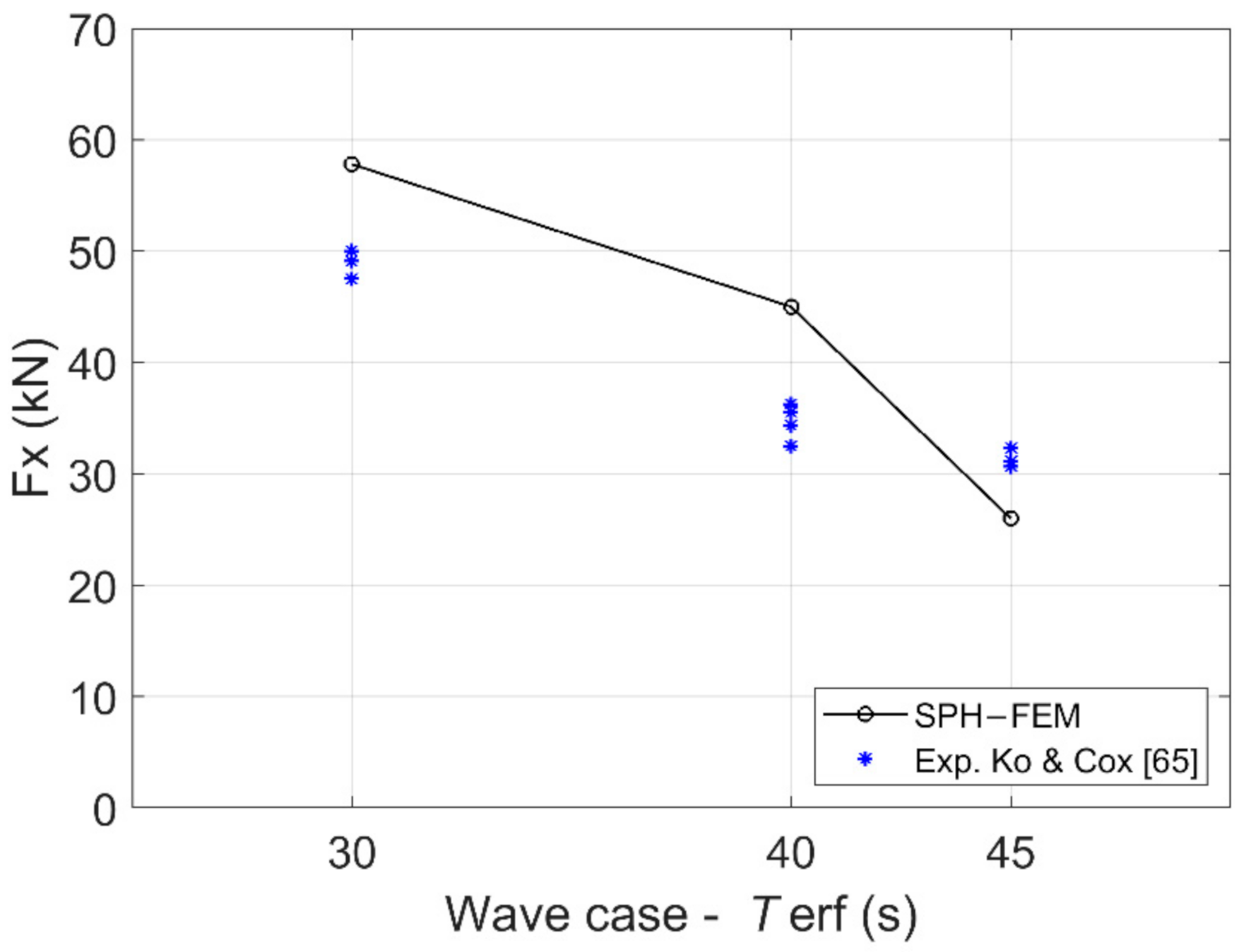
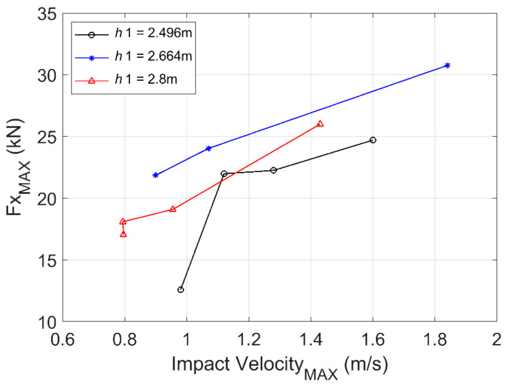
• The deviation of the numerically predicted maximum debris impact forces on the column from the experimental data was in the range of 14–25% for the investigated hydrodynamic flows. However, these differences are consistent with the observed differences in the debris impact velocities. Overall, the numerical results presented similar trends with the physical tests since both gave larger impact forces for the more transient and faster tsunami flows.

Following the verification of the numerical modeling, a preliminary investigation was conducted with the aim to gain an insight into (i) the sensitivity of the results to the debris restraints, and (ii) the role of the hydrodynamic conditions. The analyses of the 2D free debris revealed that for small water depths, the debris starts rotating clockwise upon the arrival of the bore, then as it transports inland, it changes the direction of rotation until it reaches the maximum counter-clockwise pitching angle slightly before the primary impact on the column. The prominent pitching effect during the debris transport inland resulted in higher impact velocities relatively to the restrained debris, which was unexpected, highlighting the complexity and non-linearity of the debris interaction with the turbulent flow. Moreover, despite the larger impact velocity of the free debris, the applied impact forces were smaller by approximately 56% relative to the restrained one. This is attributed to the fact that the free debris continues pitching until it reaches the column location, which results in a non-normal impact angle and a consequently non-uniform contact. This non-normal pitching angle reduces the contact area between the debris and the column, and consequently the maximum impact forces.

The comparison of different tsunami flows revealed that the 2D motion of the debris is highly dependent on the tsunami characteristics, with the largest wave (i.e., faster flow inland) causing pitching angles that were approximately 85% larger than the smallest wave. In fact, there was some indication that the pitching of the debris was caused mainly by the high velocities of the turbulent flow passing below the debris, justifying why faster bores caused more debris pitching. Moreover, the comparison of similar tsunami flows for three different water depths demonstrated that the debris–fluid interaction is also dependent on the initial water level at the debris location, with the debris pitching decreasing consistently with the increase in the water depth. When the water level is low the bottom corners of the debris can impact the bottom of the flume if the pitching angle is large, complicating further the debris–fluid interaction and impact on the column. Interestingly, although for larger water depths the relationship between the maximum debris impact force and impact velocity is nearly linear, which agrees with existing predictive equations, for the small water depth a non-linear trend was observed. In fact, in the latter case, after the exceedance of the debris velocity above a certain limit, the impact force increased less than what a linear force–velocity relationship would suggest.

Despite the limited investigated hydrodynamic conditions, the observed trends raise the question on whether debris load equations should: (i) be a function of the water depth, so that for large initial water depths a linear impact force–velocity relationship is used and for shallow depths a more complex equation is developed that will account for the debris pitching angle at the instant of impact, and/or (ii) limit the applicability of the linear force–velocity equations to a certain velocity range, above which, the rate of the force as a function of the impact velocity will drop. Future studies should consider a wider range of hydrodynamic conditions (e.g., faster flows, more water depths) and different relative distances between the debris and the coastal structure in order to determine if the pitching effects observed herein are going to be damped out as the debris propagates over longer distances. Such studies should employ 3D numerical models that will be able to simulate both the yaw and roll of the debris, in order to ensure that the influence of the pitching angle is not exaggerated by the 2D SPH–FEM models used in this study.

References

1. Yeh, H.; Sato, S.; Tajima, Y. The 11 March 2011 East Japan earthquake and tsunami: Tsunami effects on coastal infrastructure and buildings. Pure Appl. Geophys. 2013, 170, 1019–1031. [Google Scholar] [CrossRef]
2. Earthquake Engineering Research Center (EERI). The Tohoku, Japan, Tsunami of March 11, 2011: Effects on Structures, Special Earthquake Report; EERI: CA, USA, 2011; Available online: https://www.eeri.org/images/archived/wp-content/uploads/Tohoku_Japan_March_11_2011_EERI_LFE_ASCE_Tsunami_effects_on-Buildingssmallpdf.com-1.pdf (accessed on 20 September 2021).
3. FEMA P646. Guidelines for Design of Structures for Vertical Evacuation from Tsunami; Federal Emergency Management Agency: Washington, DC, USA, 2012.
4. Takahashi, S. Urgent survey for 2011 great east Japan earthquake and tsunami disaster in ports and coasts. Tech. Note Port Airpt. Res. Inst. 2011, 1231, 75–78. [Google Scholar]
5. Mikami, T.; Shibayama, T.; Esteban, M.; Matsumaru, R. Field survey of the 2011 Tohoku earthquake and tsunami in Miyagi and Fukushima prefectures. Coast. Eng. J. 2012, 54, 1250011-1–1250011-26. [Google Scholar] [CrossRef]
6. Canadian Association of Earthquake Engineering (CAEE). Reconnaissance Report on the December 26, 2004 Sumatra Earthquake and Tsunami; CAEE: British Columbia, CA, USA, 2005. [Google Scholar]
7. Akiyama, M.; Frangopol, D.M.; Strauss, A. Lessons from the 2011 Great East Japan Earthquake: Emphasis on life-cycle structural performance. In Proceedings of the Third International Symposium on Life-Cycle Civil Engineering, Vienna, Austria, 3–6 October 2012; pp. 13–20. [Google Scholar]
8. Kawashima, K.; Buckle, I. Structural performance of bridges in the Tohoku-oki earthquake. Earthq. Spectra 2013, 29, 315–338. [Google Scholar] [CrossRef]
9. Maruyama, K.; Tanaka, Y.; Kosa, K.; Hosoda, A.; Arikawa, T.; Mizutani, N.; Nakamura, T. Evaluation of tsunami force acting on bridge girders. In Proceedings of the Thirteenth East Asia-Pacific Conference on Structural Engineering and Construction, Sapporor, Japan, 11–13 September 2013; Available online: http://hdl.handle.net/2115/54508 (accessed on 15 July 2021).
10. Palermo, D.; Nistor, I.; Nouri, Y.; Cornett, A. Tsunami loading of near-shoreline structures: A primer. Can. J. Civ. Eng. 2009, 36, 1804–1815. [Google Scholar] [CrossRef]
11. Foster, A.S.J.; Rossetto, T.; Allsop, W. An experimentally validated approach for evaluating tsunami inundation forces on rectangular buildings. Coast. Eng. 2017, 128, 44–57. [Google Scholar] [CrossRef]
12. Honda, T.; Oda, Y.; Ito, K.; Watanabe, M.; Takabatake, T. An experimental study on the tsunami pressure acting on Piloti-type buildings. Coast. Eng. Proc. 2014, 1, 1–11. [Google Scholar] [CrossRef]
13. Robertson, I.N.; Riggs, H.R.; Mohamed, A. Experimental results of tsunami bore forces on structures. In Proceedings of the International Conference on Offshore Mechanics and Arctic Engineering, Shanghai, China, 6–11 January 2008; pp. 509–517. [Google Scholar] [CrossRef] [Green Version]
14. Araki, S.; Ishino, K.; Deguchi, I. Stability of girder bridge against tsunami fluid force. In Proceedings of the 32th International Conference on Coastal Engineering (ICCE), Shanghai, China, 30 June–5 July 2010. [Google Scholar]
15. Lau, T.L.; Ohmachi, T.; Inoue, S.; Lukkunaprasit, P. Experimental and Numerical Modeling of Tsunami Force on Bridge Decks; InTech: Rijeka, Croatia, 2011; pp. 105–130. [Google Scholar]
16. Hoshikuma, J.; Zhang, G.; Nakao, H.; Sumimura, T. Tsunami-induced effects on girder bridges. In Proceedings of the International Symposium for Bridge Earthquake Engineering in Honor of Retirement of Professor Kazuhiko Kawashima, Tokyo, Japan, March 2013; Available online: https://xueshu.baidu.com/usercenter/paper/show?paperid=a8a299a7f8922c5a6a312b0e8f9ad6b9&site=xueshu_se (accessed on 20 September 2021).
17. Istrati, D. Large-Scale Experiments of Tsunami Inundation of Bridges Including Fluid-Structure-Interaction. Ph.D. Thesis, University of Nevada, Reno, NV, USA, 2017. Available online: https://scholarworks.unr.edu//handle/11714/2030 (accessed on 15 July 2021).
18. Istrati, D.; Buckle, I.G.; Itani, A.; Lomonaco, P.; Yim, S. Large-scale FSI experiments on tsunami-induced forces in bridges. In Proceedings of the 16th World Conference on Earthquake, 16WCEE, Santiago, Chile, 9–13 January 2017; pp. 9–13. Available online: http://www.wcee.nicee.org/wcee/article/16WCEE/WCEE2017-2579.pdf (accessed on 15 July 2021).
19. Chock, G.Y.; Robertson, I.; Riggs, H.R. Tsunami structural design provisions for a new update of building codes and performance-based engineering. Solut. Coast. Disasters 2011, 423–435. [Google Scholar] [CrossRef]
20. Azadbakht, M.; Yim, S.C. Simulation and estimation of tsunami loads on bridge superstructures. J. Waterw. Port Coast. Ocean Eng. 2015, 141, 04014031. [Google Scholar] [CrossRef]
21. McPherson, R.L. Hurricane Induced Wave and Surge Forces on Bridge Decks. Ph.D. Thesis, Texas A&M University, College Station, TX, USA, 2008. [Google Scholar]
22. Xiang, T.; Istrati, D.; Yim, S.C.; Buckle, I.G.; Lomonaco, P. Tsunami loads on a representative coastal bridge deck: Experimental study and validation of design equations. J. Waterw. Port Coast. Ocean Eng. 2020, 146, 04020022. [Google Scholar] [CrossRef]
23. Istrati, D.; Buckle, I.G. Effect of fluid-structure interaction on connection forces in bridges due to tsunami loads. In Proceedings of the 30th US-Japan Bridge Engineering Workshop, Washington, DC, USA, 21–23 October 2014; Available online: https://www.pwri.go.jp/eng/ujnr/tc/g/pdf/30/30-10-2_Buckle.pdf (accessed on 15 July 2021).
24. Choi, S.J.; Lee, K.H.; Gudmestad, O.T. The effect of dynamic amplification due to a structure’s vibration on breaking wave impact. Ocean Eng. 2015, 96, 8–20. [Google Scholar] [CrossRef]
25. Bozorgnia, M.; Lee, J.J.; Raichlen, F. Wave structure interaction: Role of entrapped air on wave impact and uplift forces. In Proceedings of the International Conference on Coastal Engineering, 30 June–5 July 2010. [Google Scholar]
26. Seiffert, B.; Hayatdavoodi, M.; Ertekin, R.C. Experiments and computations of solitary-wave forces on a coastal-bridge deck. Part I: Flat plate. Coast. Eng. 2014, 88, 194–209. [Google Scholar] [CrossRef]
27. Xu, G.; Cai, C.S.; Chen, Q. Countermeasure of air venting holes in the bridge deck–wave interaction under solitary waves. J. Perform. Constr. Facil. 2017, 31, 04016071. [Google Scholar] [CrossRef]
28. Istrati, D.; Buckle, I. Role of trapped air on the tsunami-induced transient loads and response of coastal bridges. Geosciences 2019, 9, 191. [Google Scholar] [CrossRef] [Green Version]
29. Istrati, D.; Buckle, I.; Lomonaco, P.; Yim, S. Deciphering the tsunami wave impact and associated connection forces in open-girder coastal bridges. J. Mar. Sci. Eng. 2018, 6, 148. [Google Scholar] [CrossRef] [Green Version]
30. Seiffert, B.R.; Cengiz Ertekin, R.; Robertson, I.N. Effect of entrapped air on solitary wave forces on a coastal bridge deck with girders. J. Bridge Eng. 2016, 21, 04015036. [Google Scholar] [CrossRef]
31. Rossetto, T.; Peiris, N.; Pomonis, A.; Wilkinson, S.M.; Del Re, D.; Koo, R.; Gallocher, S. The Indian Ocean tsunami of december 26, 2004: Observations in Sri Lanka and Thailand. Nat. Hazards 2007, 42, 105–124. [Google Scholar] [CrossRef]
32. Robertson, I.N.; Carden, L.; Riggs, H.R.; Yim, S.; Young, Y.L.; Paczkowski, K.; Witt, D. Reconnaissance following the September 29, 2009 tsunami in Samoa. Res. Rep. 2010. Available online: https://www.eeri.org/site/images/eeri_newsletter/2010_pdf/Samoa-Rpt.pdf (accessed on 15 July 2021).
33. Yeom, G.S.; Nakamura, T.; Mizutani, N. Collision analysis of container drifted by runup tsunami using drift collision coupled model. J. Disaster Res. 2009, 4, 441–449. [Google Scholar] [CrossRef]
34. Madurapperuma, M.A.K.M.; Wijeyewickrema, A.C. Inelastic dynamic analysis of an RC building impacted by a tsunami water-borne shipping container. J. Earthq. Tsunami 2012, 6, 1250001. [Google Scholar] [CrossRef]
35. Como, A.; Mahmoud, H. Numerical evaluation of tsunami debris impact loading on wooden structural walls. Eng. Struct. 2013, 56, 1249–1261. [Google Scholar] [CrossRef]
36. Haehnel, R.B.; Daly, S.F. Maximum impact force of woody debris on floodplain structures. J. Hydraul. Eng. 2004, 130, 112–120. [Google Scholar] [CrossRef]
37. Ko, H. Hydraulic Experiments on Impact Forces from Tsunami-Driven Debris. Master’s Thesis, Oregon State University, Corvallis, OR, USA, 2013. [Google Scholar]
38. Shafiei, S.; Melville, B.W.; Shamseldin, A.Y.; Adams, K.N.; Beskhyroun, S. Experimental investigation of tsunami-borne debris impact force on structures: Factors affecting impulse-momentum formula. Ocean Eng. 2016, 127, 158–169. [Google Scholar] [CrossRef]
39. Stolle, J.; Goseberg, N.; Nistor, I.; Petriu, E. Debris impact forces on flexible structures in extreme hydrodynamic conditions. J. Fluids Struct. 2019, 84, 391–407. [Google Scholar] [CrossRef]
40. Derschum, C.; Nistor, I.; Stolle, J.; Goseberg, N. Debris impact under extreme hydrodynamic conditions part 1: Hydrodynamics and impact geometry. Coast. Eng. 2018, 141, 24–35. [Google Scholar] [CrossRef]
41. Yang, W.C. Study of Tsunami-Induced Fluid and Debris Load on Bridges using the Material Point Method. Ph.D. Thesis, University of Washington, Seattle, WA, USA, 2016. Available online: http://hdl.handle.net/1773/37064 (accessed on 15 July 2021).
42. Oudenbroek, K.; Naderi, N.; Bricker, J.D.; Yang, Y.; Van der Veen, C.; Uijttewaal, W.; Moriguchi, S.; Jonkman, S.N. Hydrodynamic and debris-damming failure of bridge decks and piers in steady flow. Geosciences 2018, 8, 409. [Google Scholar] [CrossRef] [Green Version]
43. Istrati, D.; Hasanpour, A.; Buckle, I. Numerical Investigation of Tsunami-Borne Debris Damming Loads on a Coastal Bridge. In Proceedings of the 17 World Conference on Earthquake Engineering, Sendai, Japan, 13–18 September 2020. [Google Scholar]
44. Istrati, D.; Buckle, I.G. Tsunami Loads on Straight and Skewed Bridges—Part 1: Experimental Investigation and Design Recommendations (No. FHWA-OR-RD-21-12). Oregon Department of Transportation. Research Section. 2021. Available online: https://rosap.ntl.bts.gov/view/dot/55988 (accessed on 15 July 2021).
45. St-Germain, P.; Nistor, I.; Townsend, R.; Shibayama, T. Smoothed-particle hydrodynamics numerical modeling of structures impacted by tsunami bores. J. Waterw. Port Coast. Ocean Eng. 2014, 140, 66–81. [Google Scholar] [CrossRef]
46. Pringgana, G.; Cunningham, L.S.; Rogers, B.D. Modelling of tsunami-induced bore and structure interaction. Proc. Inst. Civ. Eng.-Eng. Comput. Mech. 2016, 169, 109–125. [Google Scholar] [CrossRef] [Green Version]
47. Sarfaraz, M.; Pak, A. SPH numerical simulation of tsunami wave forces impinged on bridge superstructures. Coast. Eng. 2017, 121, 145–157. [Google Scholar] [CrossRef]
48. Zhu, M.; Elkhetali, I.; Scott, M.H. Validation of OpenSees for tsunami loading on bridge superstructures. J. Bridge Eng. 2018, 23, 04018015. [Google Scholar] [CrossRef]
49. Liu, G.R.; Liu, M.B. Smoothed Particle Hydrodynamics: A Meshfree Particle Method; World Scientific: Singapore, 2003. [Google Scholar]
50. Violeau, D. Fluid Mechanics and the SPH Method: Theory and Applications; Oxford University Press: Oxford, UK, 2012. [Google Scholar]
51. Monaghan, J.J.; Kos, A. Solitary waves on a Cretan beach. J. Waterw. Port Coast. Ocean Eng. 1999, 125, 145–155. [Google Scholar] [CrossRef]
52. Colagrossi, A.; Landrini, M. Numerical simulation of interfacial flows by smoothed particle hydrodynamics. J. Comput. Phys. 2003, 191, 448–475. [Google Scholar] [CrossRef]
53. Monaghan, J.J.; Kos, A.; Issa, N. Fluid motion generated by impact. J. Waterw. Port Coast. Ocean Eng. 2003, 129, 250–259. [Google Scholar] [CrossRef]
54. Crespo, A.J.C.; Gómez-Gesteira, M.; Dalrymple, R.A. 3D SPH simulation of large waves mitigation with a dike. J. Hydraul. Res. 2007, 45, 631–642. [Google Scholar] [CrossRef]
55. Pelfrene, J. Study of the SPH Method for Simulation of Regular and Breaking Waves. Master’s Thesis, Gent University, Ghent, Belgium, 2011. [Google Scholar]
56. Dalrymple, R.A.; Knio, O.; Cox, D.T.; Gesteira, M.; Zou, S. Using a Lagrangian particle method for deck overtopping. Ocean Wave Meas. Anal. 2002, 1082–1091. [Google Scholar] [CrossRef]
57. Gómez-Gesteira, M.; Dalrymple, R.A. Using a three-dimensional smoothed particle hydrodynamics method for wave impact on a tall structure. J. Waterw. Port Coast. Ocean Eng. 2004, 130, 63–69. [Google Scholar] [CrossRef]
58. Barreiro, A.; Crespo, A.J.C.; Domínguez, J.M.; Gómez-Gesteira, M. Smoothed particle hydrodynamics for coastal engineering problems. Comput. Struct. 2013, 120, 96–106. [Google Scholar] [CrossRef]
59. Altomare, C.; Crespo, A.J.; Domínguez, J.M.; Gómez-Gesteira, M.; Suzuki, T.; Verwaest, T. Applicability of Smoothed Particle Hydrodynamics for estimation of sea wave impact on coastal structures. Coast. Eng. 2015, 96, 1–12. [Google Scholar] [CrossRef]
60. Aristodemo, F.; Tripepi, G.; Meringolo, D.D.; Veltri, P. Solitary wave-induced forces on horizontal circular cylinders: Laboratory experiments and SPH simulations. Coast. Eng. 2017, 129, 17–35. [Google Scholar] [CrossRef]
61. Gómez-Gesteira, M.; Cerqueiro, D.; Crespo, C.; Dalrymple, R.A. Green water overtopping analyzed with a SPH model. Ocean Eng. 2005, 32, 223–238. [Google Scholar] [CrossRef]
62. Yang, Y.; Li, J. SPH-FE-Based Numerical Simulation on Dynamic Characteristics of Structure under Water Waves. J. Mar. Sci. Eng. 2020, 8, 630. [Google Scholar] [CrossRef]
63. Hu, D.; Long, T.; Xiao, Y.; Han, X.; Gu, Y. Fluid–structure interaction analysis by coupled FE–SPH model based on a novel searching algorithm. Comput. Methods Appl. Mech. Eng. 2014, 276, 266–286. [Google Scholar] [CrossRef] [Green Version]
64. Thiyahuddin, M.I.; Gu, Y.; Gover, R.B.; Thambiratnam, D.P. Fluid–structure interaction analysis of full scale vehicle-barrier impact using coupled SPH–FEA. Eng. Anal. Bound. Elem. 2014, 42, 26–36. [Google Scholar] [CrossRef] [Green Version]
65. Ko, H.; Cox, D. OSU: 1-D Hydraulic Experiment, Aluminum, Water depth = 249.6 cm. DesignSafe-CI 2012. [Google Scholar] [CrossRef]
66. Hallquist, J.O. LS-DYNA theory manual. Liverm. Softw. Technol. Corp. 2006, 3, 25–31. [Google Scholar]
67. Grimaldi, A.; Benson, D.J.; Marulo, F.; Guida, M. Steel structure impacting onto water: Coupled finite element-smoothed-particle-hydrodynamics numerical modeling. J. Aircr. 2011, 48, 1299–1308. [Google Scholar] [CrossRef]
68. Panciroli, R.; Abrate, S.; Minak, G.; Zucchelli, A. Hydroelasticity in water-entry problems: Comparison between experimental and SPH results. Compos. Struct. 2012, 94, 532–539. [Google Scholar] [CrossRef]
69. Monaghan, J.J. Simulating free surface flows with SPH. J. Comput. Phys. 1994, 110, 399–406. [Google Scholar] [CrossRef]
70. Wu, Z. Compactly supported positive definite radial functions. Adv. Comput. Math. 1995, 4, 283–292. [Google Scholar] [CrossRef]
71. Monaghan, J.J.; Lattanzio, J.C. A refined particle method for astrophysical problems. Astron. Astrophys. 1985, 149, 135–143. [Google Scholar]
72. Gingold, R.A.; Monaghan, J.J. Smoothed particle hydrodynamics: Theory and application to non-spherical stars. Mon. Notices R. Astron. Soc. 1977, 181, 375–389. [Google Scholar] [CrossRef]
73. Das, J.; Holm, H. On the improvement of computational efficiency of smoothed particle hydrodynamics to simulate flexural failure of ice. J. Ocean Eng. Mar. Energy 2018, 4, 153–169. [Google Scholar] [CrossRef]
74. Petschek, A.G.; Libersky, L.D. Cylindrical smoothed particle hydrodynamics. J. Comput. Phys. 1993, 109, 76–83. [Google Scholar] [CrossRef]
75. Monaghan, J.J.; Gingold, R.A. Shock simulation by the particle method SPH. J. Comput. Phys. 1983, 52, 374–389. [Google Scholar] [CrossRef]
76. Xu, J.; Wang, J. Node to node contacts for SPH applied to multiple fluids with large density ratio. In Proceedings of the 9th European LS-DYNA Users’ Conference, Manchester, UK, 3 June 2013; pp. 2–4. [Google Scholar]
77. Thomas, S.; Cox, D. Influence of finite-length seawalls for tsunami loading on coastal structures. J. Waterw. Port Coast. Ocean Eng. 2012, 138, 203–214. [Google Scholar] [CrossRef]
78. Swegle, J.W.; Attaway, S.W.; Heinstein, M.W.; Mello, F.J.; Hicks, D.L. An analysis of smoothed particle hydrodynamics (No. SAND-93-2513). Sandia Natl. Labs 1994. [Google Scholar] [CrossRef] [Green Version]
79. American Society of Civil Engineers (ASCE). Minimum Design Loads and Associated Criteria for Buildings and Other Structures; ASCE/SEI 7-16; American Society of Civil Engineers (ASCE): Reston, VA, USA, 2016. [Google Scholar]
80. Istrati, D.; Buckle, I.G. Tsunami Loads on Straight and Skewed Bridges—Part 2: Numerical Investigation and Design Recommendations (No. FHWA-OR-RD-21-13). Oregon Department of Transportation. Research Section. 2021. Available online: https://rosap.ntl.bts.gov/view/dot/55947 (accessed on 15 July 2021).
81. Stolle, J.; Nistor, I.; Goseberg, N.; Petriu, E. Multiple Debris Impact Loads in Extreme Hydrodynamic Conditions. J. Waterw. Port Coast. Ocean Eng. 2020, 146, 04019038. [Google Scholar] [CrossRef]
82. Goseberg, N.; Stolle, J.; Nistor, I.; Shibayama, T. Experimental analysis of debris motion due the obstruction from fixed obstacles in tsunami-like flow conditions. Coast. Eng. 2016, 118, 35–49. [Google Scholar] [CrossRef]
Figure 1. Cross-section of the Large Wave Flume (LWF) depicting the bathymetry, column location and flume instrumentation of the experiments of Ko and Cox [65] used for the validation study.
Jmse 09 01068 g001
Figure 2. Numerical models with large debris: side-views of the debris, the column and the wave maker.
Jmse 09 01068 g002
Figure 3. Variation of the free surface and fluid velocity at different locations along the flume. Experimental [65] and numerical results for h1 = 2.496 m and Terf = 30 s.
Jmse 09 01068 g003
Figure 4. Maximum free-surface values of experiments [65] and numerical simulations for h1 = 2.496 m, and three wave cases with Terf = 30, 40 and 45 s.
Jmse 09 01068 g004
Figure 5. Maximum fluid velocities of experimental tests [65] and numerical simulations for h1 = 2.496 m, and three wave cases with Terf = 30, 40, and 45 s.
Jmse 09 01068 g005
Figure 6. Debris velocity histories: Estimated based on the experimental tests of [65] and results from the numerical simulations for h1 = 2.496 m, Terf = 30 s.
Jmse 09 01068 g006
Figure 7. Comparison of the debris impact forces: experimental tests [65] and numerical simulations for h1 = 2.496 m, and two wave cases with Terf = 30 s and 45 s.
Jmse 09 01068 g007
Figure 8. Maximum values of debris impact force on column: experimental tests [65] and numerical simulation for h1 = 2.496 m, and three wave cases with Terf = 30, 40, and 45 s.
Jmse 09 01068 g008
Figure 9. Selected instants of the debris−wave interaction and impact on the column of the free debris. Numerical results for the hydrodynamic case with h1 = 2.496 m, h2 = 0.13 m and Terf = 30 s.
Jmse 09 01068 g009
Figure 10. Debris trajectory (left) and rotation (right) for the restrained debris and free debris. Numerical results for the hydrodynamic case with h1 = 2.496 m, and h2 = 0.13 m and Terf = 30 s.
Jmse 09 01068 g010
Figure 11. Debris velocity (left) and forces on the column (right). Experimental and numerical results (of restrained and free debris) for the hydrodynamic case h1 = 2.496 m and Terf = 30 s.
Jmse 09 01068 g011
Figure 12. Variation of free surface (left) and fluid velocity (right) at x = 62 m: Numerical results for h1 = 2.496 m and three wave cases with Terf = 30, 40, and 45 s.
Jmse 09 01068 g012
Figure 13. Snapshots of debris−tsunami interaction and impact on the column. Numerical results for h1 = 2.496 m and two wave cases with Terf = 30 s (top) and 45 s (bottom).
Jmse 09 01068 g013
Figure 14. Numerical results of the free debris: vertical displacement (left) and rotation (right), for h1 = 2.496 m and three wave cases with Terf = 30, 40, and 45 s.
Jmse 09 01068 g014
Figure 15. Free−debris histories (left) and maximum values of debris impact on the column vs. the impact velocity (right). Numerical results for h1 = 2.496 m h2 = 0.13 m, and Terf = 30, 40, and 45 s.
Jmse 09 01068 g015
Figure 16. Time histories of the free surface, fluid velocity, motion of the debris (y displacement and rotation), debris velocity and debris impact force on the column. Numerical results of free debris for Terf = 40 s and three water depths with h1 = 2.496, 2.664 and 2.8 m.
Jmse 09 01068 g016
Figure 17. Snapshots of debris-tsunami interaction and impact on the column. Numerical results of free debris for Terf = 40 s and three water depths with h1 = 2.496 (top), 2.664 (center) and 2.8 m (bottom).
Jmse 09 01068 g017
Figure 18. Maximum values of the debris impact force as a function of the impact velocity for three water depths and nine tsunami bores.
Jmse 09 01068 g018
Publisher’s Note: MDPI stays neutral with regard to jurisdictional claims in published maps and institutional affiliations.