Fuel Consumption and Emissions of Ocean-Going Cargo Ship with Hybrid Propulsion and Different Fuels over Voyage

Abstract

Hybrid propulsion and using liquefied natural gas (LNG) as the alternative fuel have been applied on automobiles and some small ships, but research investigating the fuel consumption and emissions over the total voyage of ocean-going cargo ships with a hybrid propulsion and different fuels is limited. This paper tries to fill the knowledge gap by investigating the influence of the ship mission profile, propulsion modes and effects of different fuels on the fuel consumption and emissions of the ship over the whole voyage, including transit in open sea and manoeuvring in close-to-port areas. Results show that propulsion control and electric power generation modes have a notable influence on the ship’s fuel consumption and emissions during the voyage. During close-to-port manoeuvres, propelling the ship in power-take-in (PTI) mode and generating the electric power by auxiliary engines rather than the main engine will reduce the local NOx and HC (hydrocarbons) emissions significantly. Sailing the ship on LNG will reduce the fuel consumption, CO₂ and NOx emissions notably while producing higher HC emissions than traditional fuels. The hybridisation of the ship propulsion and using LNG together with ship voyage optimisation, considering the ship mission, ship operations and sea conditions, will improve the ship’s fuel consumption and emissions over the whole voyage significantly.

1. Introduction

Shipping, which is a relatively energy-efficient, environment-friendly and sustainable mode of mass transport of cargo [1], is the dominant and will remain the most important transport mode for world trade [2]. However, the shipping industry consumes more fuel in comparison with other transport modes [3] and shipping-related emissions contribute significantly to the global air pollution and long-term global warming [4,5]. Correlated with fuel consumption, shipping is responsible for approximately 3.1% of annual global CO₂ and approximately 2.8% of annual GHGs (greenhouse gases) on a CO₂e (CO₂ equivalent) basis [6]. Approximately 15% and 13% of global human-made NOx and SOx emissions come from the shipping industry. It is projected that maritime CO₂ emissions will increase significantly by 50% to 250% in the period up to 2050 [6]. Moreover, as fuel cost accounts for approximately 50% to 60% of the total operational cost of a ship [7], a significant fuel consumption reduction will contribute to a considerable save of a ship’s operational cost. Consequently, the shipping industry is striving to reduce its fuel consumption and emissions due to the increasingly high fuel price, social concerns on the environmental impact and the resulting mandatory and strict emission control regulations worldwide [8].

Ship mission profile during the voyage has a significant influence on the fuel consumption and exhaust emissions of ships [9]. Therefore, the ship mission profiles should be taken into consideration when evaluating ship transport performance [10]. However, one of the major drawbacks of the present IMO (International Maritime Organization)’s EEDI (Energy Efficiency Design Index) is that it only considers one operating point without taking the ship’s representative mission profiles into account. On the contrary, the EEOI (energy efficiency operational indicator), which is also developed by IMO, is calculated for a voyage or a number of voyage legs based on real operating conditions [11]. In [12], based on a case study of a handy size Chemical/Product Tanker of 38,000 DWT (Deadweight tonnage), Acomi, et al. investigate the voyage energy efficiency by calculating the EEOI of the ship using both commercial software and onboard measures. In [13], in the case study of a RoPax vessel, Coraddu et al. estimate the ship operational performance of the ship voyage using the EEOI as the measure by real data statistics and numerical simulations. In [14], Hou et al. optimise the vessel speed of an ice zone ship to find a minimum EEOI in an ice zone. In [15], in the case study of a VLCC (Very Large Crude Carrier) tanker, Safaei et al. address the reduction in fuel consumption of the ship voyage using route optimisation considering ship profile and sea conditions. In [16], in the case study of a bulk carrier, Zaccone et al. develop a 3D dynamic programming optimisation method to select the optimal path and speed profile for the ship voyage aiming to minimise the voyage fuel consumption and taking also into account ship safety and comfort. However, most of the research focuses on route planning and ship speed profile when studying the ship voyage optimisation. During ship operation, propulsion control [17,18], power management [19,20,21] and ship operational speeds [22,23] will significantly influence the fuel consumption and emissions performance of ships. However, quantitative and systematic investigations on the influence of various ship operations, including propulsion control, power management and operational speeds, on the ship performance of the whole voyage are still limited.

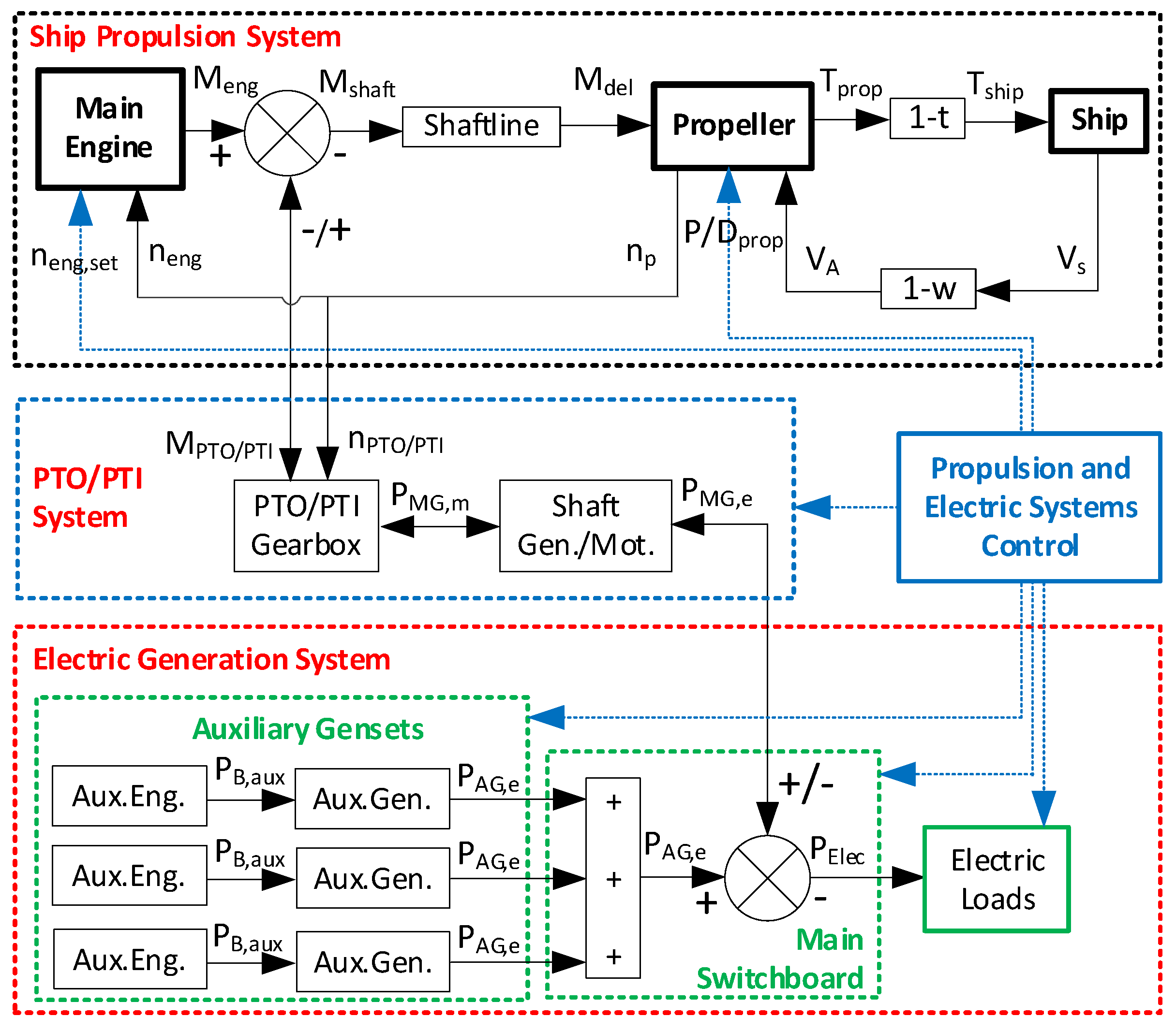
Hybrid propulsion, which is a combination of mechanical and electrical propulsion, is a promising option to improve the economic, environmental and operational performance of ships [24,25]. In the basic form of the hybrid propulsion system, the propeller can be mechanically driven by an internal combustion engine and/or electrically driven by an electric motor, which may also be able to work as an electric generator. If the electric motor is powered by a hybrid power supply, such as diesel generator(s), natural gas generator(s), fuel cells and/or batteries, it will be a hybrid propulsion with a hybrid power supply system [26]. The operation modes of a hybrid propulsion system include power take off (PTO); slow power take in (PTI); boost power take in [27]. Among others, the benefits of a hybrid propulsion include reduced fuel consumption; reduced CO2 emissions and other pollutants; possibility to sail and operate with zero emission in coastal and port areas; greater redundancy; noise reduction; lower maintenance [24,28]. However, different ship types can benefit differently from the hybrid propulsion due to their diverse operational profiles [28,29]. In [29], Jafarzadeh and Schjølberg study the operational profiles of eight different ship types, including tankers, bulk carriers, general cargo ships, container ships, Ro-Ro ships, reefers, offshore ships and passenger ships, aiming to identify what ship types are able to benefit from hybrid propulsion. Hybrid ship propulsion is typically applied on naval vessels, towing vessels, offshore vessels and passenger ships including ferries. However, the current applications and research of hybrid propulsion are mainly limited on small ships, while the applications and research on large ocean-going vessels are rare.

To improve the safety and operability of ocean-going cargo ships and to reduce their global greenhouse gas emissions and the local pollutant emissions in coastal and port areas, few studies on the potential applications of hybrid propulsion and power supply system on the big ocean-going cargo ships can be found. In [30], based on a multi-physical domain model, a conceptual hybrid propulsion system for a very large crude oil carrier (VLCC) has been studied for the potential benefit of improving the ship’s safety and operability in heavy sea conditions without reducing the system efficiency. In [31] and [32], the potential benefits of hybrid propulsion for large ocean-going cargo vessels to increase fuel efficiency and reduce greenhouse gas emissions and pollutant emissions are investigated as well. In [33], the impact of battery–hybrid propulsion on the fuel consumption and emissions of an ocean-going chemical tanker when sailing in coastal and port areas during port approaches has been investigated. However, it is concluded that the battery–hybrid propulsion for ocean-going cargo ships, even when only sailing at low ship speed in close-to-port areas for a short time, is still not a realistic option nowadays even though it can produce zero local emissions; the main reason is that the required battery capacity is very large and the weight of the battery becomes unacceptable.

Using LNG (liquefied natural gas) as the alternative marine fuel is another promising and attractive solution to reducing the local and regional environmental impact and operational costs of ships [34,35]. Compared to using conventional marine fuels, using LNG produces significantly less pollutant emissions, such as NOx, SOx and PM (particle matter), and CO₂ emissions will also be reduced as well [24,36]. Another driver for using LNG as a marine fuel is the current favourable fuel price compared to the increasing price of conventional fuel oil [37]. However, one of the disadvantages in the use of LNG as marine fuel is that it may have a worse impact on climate change (global warming) than using conventional fuels, when taking the life-cycle emissions of methane (CH₄), which is a worse greenhouse gas than CO₂, into consideration [35,37]. Currently, a relatively small number of ships run on LNG and adopting LNG as a fuel is attractive for ships sailing on fixed routes and large ships sailing in short sea and coastal areas, especially in emission control areas (ECAs) [38,39,40]. With more stricter emissions regulations coming into force and more infrastructure of LNG fuel growing worldwide, larger ocean-going vessels are expected to select LNG as a fuel in the foreseeable future [39]. There are many publications indicating the potential benefits of using LNG as a marine fuel, however, quantitative investigations on the impact of using LNG as a fuel on the fuel consumption and emissions of ships over the whole voyage, taking the ship’s operational profile into consideration, are limited.

This paper will therefore investigate the potential influence of the application of the hybrid ship propulsion and electric power generation system with different fuels as well as various propulsion control and power management strategies on the ocean-going cargo ship in reducing the fuel consumption and emissions over the whole voyage.

The main goals and outline of this paper are:

(1)

To introduce the conceptual hybrid propulsion and electric power generation system of a benchmark ocean-going chemical tanker (Section 2).

(2)

To explain the “average” indicators of the fuel consumption and emissions performance of the ship taking the ship mission profiles of both the transit voyage in open sea and manoeuvre in close-to-port areas into consideration (Section 3).

(3)

To present the fuel consumption and emissions models of both the main engine (two-stroke diesel engine) and the auxiliary engines (four-stroke diesel engine) as well as the model corrections on different fuel types (Section 4).

(4)

To introduce the ship mission profiles of the transit voyage sailing in open sea and the close-to-port manoeuvre in coastal and port areas (Section 5).

(5)

To quantitatively and systematically investigate the influence of the ship operational speeds, propulsion control modes, electric power generation modes, sailing on different fuel types and PTI propulsion mode on the fuel consumption and emissions performance over the whole voyage, including the transit in open sea and manoeuvre in close-to-port areas (Section 6).

In Section 7, the conclusions, limitations and uncertainties of the present paper and the recommendations for future work will be provided.

2. Hybridisation of the Benchmark Chemical Tanker

The ocean-going 13,000 DWT chemical tanker introduced in [41] has been chosen to investigate the fuel consumption and emissions performance of the ship when transiting in open sea and manoeuvring in coastal and port areas. The propulsion system of the chemical tanker consists of a two-stroke diesel engine working as the main engine, a controllable pitch propeller (CPP) and the shafting system. The electric power generation system includes a shaft generator (power take off, PTO) driven by the main engine and three auxiliary generators. The ship particulars of the chemical tanker are given in

Table 1. Ship particulars of the benchmark chemical tanker.

Length Between Perpendiculars (m)	113.80
Breadth Molded (m)	22.00
Depth Molded (m)	11.40
Design Draught (m)	8.50
Design Displacement (m3)	16,988
Dead Weight Tonnage (ton)	13,000
Design Ship Speed (kn)	13.30

and the particulars of the main engine (two-stroke diesel engine) and auxiliary engines (four-stroke diesel engine) are given in

Table 2. Particulars of the main engine and auxiliary engines.

Parameters	Main Engine	Auxiliary Engine
Engine Type	MAN 6S35ME-B9.3-TII (2-stroke)	DAIHATSU 6DE-18 (4-stroke)
Number of engines (-)	1	3
Rated Power (kW)	4170	750
Rated Speed (rpm)	167	900
Stroke (m)	1.55	0.28
Bore (m)	0.35	0.185
Mean Effective Pressure (MPa)	1.67	2.21

.

In the benchmark ship, originally, the shaft generator can only work in PTO mode. In order to investigate the potential fuel consumption and emissions performance of a hybrid ocean-going cargo ship especially when sailing in coastal and harbour areas, in this paper, the original propulsion system and electric power generation system of the benchmark chemical tanker have been conceptually hybridised. In the conceptual hybrid ship propulsion and electric power generation system (Figure 1), the shaft generator can also work as a shaft motor in PTI (power take in) mode. To investigate the influence of sailing on different fuels on the fuel consumption and emissions of the ship, both the main engine and auxiliary engines have been assumed (conceptually updated) so that they can also use LNG (liquefied natural gas) as their fuels, without considering the details of how the engines will be updated and how different fuels will be stored and managed onboard the ship, which are out of the scope of this paper. So, after the updates, the benchmark ocean-going chemical tanker will have a hybrid ship propulsion and electric generation system.

3. Mean Value Indicators of Fuel Consumption and Emissions

The mean value indicators of fuel consumption and emissions presented and used in this paper are defined based on the theories introduced in [10,33,41]. When taking the ship mission profile into account and in order to express the ship performance as a single value, an operational average value of energy effectiveness and energy (fuel) index has been introduced in [10].

The mean energy conversion effectiveness ${\overline{\epsilon }}_{EC}$ over voyage, which is the weighted average value over the mission profile of the ship that will be defined later in the following chapter, is defined in Equation (1).

$${\overline{\epsilon }}_{EC}=\frac{{\displaystyle \sum _i{W}_{D,i}\cdot V_i\cdot \Delta t_i}}{{\displaystyle \sum _i\left({\Phi }_{FE,main,i}+{\Phi }_{FE,aux,i}\right)\cdot \Delta t_i}}$$

(1)

where $W_{D,i}$, $V_i$, ${\Phi }_{FE,main,i}$, ${\Phi }_{FE,aux,i}$ and $\Delta t_i$ are the ship dead weight (N), ship speed (m/s), energy flow into main engine (J/s), energy flow into auxiliary engines (J/s) and time of duration in each part of the voyage (h).

Same as for the definition of the mean energy conversion effectiveness, the mean fuel index $\overline{FI}$ (g/(ton·mile)) and mean emission index $\overline{EI}$ (g/(ton·mile)) averaged over the whole voyage of the ship are defined by Equations (2) and (3), respectively [33].

$$\overline{FI}=\frac{{\displaystyle \sum _i\left({\Phi }_{Fuel,main,i}+{\Phi }_{Fuel,aux,i}\right)\cdot \Delta t_i}}{{\displaystyle \sum _i{M}_{D,i}\cdot V_i\cdot \Delta t_i}}$$

(2)

$$\overline{EI}=\frac{{\displaystyle \sum _i\left({\Phi }_{Emission,main,i}+{\Phi }_{Emission,aux,i}\right)\cdot \Delta t_i}}{{\displaystyle \sum _i{M}_{D,i}\cdot V_i\cdot \Delta t_i}}$$

(3)

where ${\Phi }_{Fuel,main,i}$, ${\Phi }_{Fuel,aux,i}$, ${\Phi }_{Emission,main,i}$, ${\Phi }_{Emission,aux,i}$ and $M_{D,i}$ are the fuel mass flow into the main engine (g/h), fuel mass flow into auxiliary engines (g/h), emission mass flow generated by the main engine (g/h), emission mass flow generated by auxiliary engines (g/h) and dead weight tonnage of the ship (t) in each part of the voyage, respectively.

4. Mathematical Models

The ship propulsion and electric generation system model of the benchmark chemical tanker introduced in [41] has been updated in this paper and the model structure is shown in Figure 2. The models of fuel consumption and emissions of diesel engines will be briefly presented in this paper. The models of ship resistance, propeller open water characteristics, wake factor, thrust deduction factor and relative rotative efficiency can be found in [41] for detail. The onboard electric loads are modelled by a constant value, which is set as 350 kW. The shaft generator/motor and the auxiliary generators are modelled by constant energy conversion efficiencies (which is consistent with the constant auxiliary power assumption and the practice of switching on/off auxiliary generators to ensure proper loading of the engines). The energy conversion efficiencies of both the generator(s) and motor are set as 95% in the model.

4.1. Models of Fuel Consumption and Emissions of Diesel Engines

The fuel consumption is calculated using the engine torque model introduced in [3], in which the engine torque is modelled as a function of the fuel consumption and engine speed in the form of second order Taylor expansion of two variables, including the cross product, as shown in Equation (4). Similarly, the emissions are modelled as functions of the engine torque and engine speed [33] as shown in Equation (5). The constant coefficients in the models can be fitted using engine test data.

$$\begin{array}{l}{M}^{*}=f_1\left(m_f^{*},N^{*}\right)\\ =1-a\cdot \left(1-m_f^{*}\right)+b\cdot {\left(1-m_f^{*}\right)}^2-c\cdot \left(1-N^{*}\right)+d\cdot {\left(1-N^{*}\right)}^2+2\cdot e\cdot \left(1-m_f^{*}\right)\cdot \left(1-N^{*}\right)\end{array}$$

(4)

$$\begin{array}{l}{\Phi }_{em}^{*}=f_2\left(M^{*},N^{*}\right)\\ =1-a_{em}\cdot \left(1-N^{*}\right)+b_{em}\cdot {\left(1-N^{*}\right)}^2-c_{em}\cdot \left(1-M^{*}\right)+d_{em}\cdot {\left(1-M^{*}\right)}^2+2\cdot e_{em}\cdot \left(1-N^{*}\right)\cdot \left(1-M^{*}\right)\end{array}$$

(5)

where $M^{*}$, $N^{*}$, $m_f^{*}$ and ${\Phi }_{em}^{*}$ are the normalised engine torque, engine speed, fuel mass injected per cycle, emission mass flow, which are normalised by dividing the relevant variables using the corresponding nominal value of the variables.

Only the emissions of the carbon dioxide CO₂, NOx and HC (hydrocarbons) are investigated in this paper. The carbon dioxide is the direct product of the complete combustion of the fuel. So, the CO₂ emission is directly determined by the fuel consumption. Note that, as the test data of the auxiliary engines installed in the benchmark ship is not available, the fuel consumption and emissions models of the auxiliary engines are calibrated using the average data of (a small number of) similar engines that are available in the internal dataset. The calibration of the model of the main engine using the engine test data has been introduced in detail in [41]. More details on the calibration of the NOx and HC emissions models of the main engine and auxiliary engines can be found in Appendix B.

4.2. Corrections for Different Fuel Types

The test results of fuel consumption and emissions for developing and calibrating the models of both the main engine and the auxiliary engines have been corrected at ISO (International Organization for Standardization) standard reference conditions using the standard LHV (Lower Heating Value) of the fuel oil (42,700 kJ/kg), referring to ISO 15550:2016 and ISO 3046-1:2002. However, in this paper, the influence of sailing on different fuel types on the ship fuel consumption and emissions will be investigated. For instance, when the ship is in operation, the fuel type for the main engine can be HFO (heavy fuel oil), MDF (marine diesel fuel) or LNG (liquefied natural gas); while the fuel type for the auxiliary engines can be MDF (marine diesel fuel) or LNG (liquefied natural gas). Therefore, the fuel consumption, NOx emission and HC emission during ship operations need to be corrected accordingly by Equation (6) using the multiplying correcting factors shown in

Table 3. Correcting factors of fuel consumption and NOx and HC emissions.

Fuel Type	ISO *	HFO *	MDF *	LNG *
LHV (kJ/kg)	42,700	41,500	42,000	48,000 (+/− 2000)
$C_{fuel}$ (-)	1	1.0289	1.0167	0.8896 (+/− 0.047)
$C_{NOx}$ (-)	1	1.2	1.0	0.2 (+/− 0.1)
$C_{HC}$ (-)	1	1.5	1.0	10.0 (+/− 6)

* ISO, ISO standard reference conditions, referring to ISO 15550:2016 and ISO 3046-1:2002. HFO, heavy fuel oil; MDF, marine diesel fuel; LNG, liquefied natural gas; LHV, lower heat values.

(and uncertainty in these factors which is in between brackets).

The underlying assumption for correcting the fuel consumption is that the efficiencies of the engines remain the same when the fuel types are changed. The correcting factors for NOx and HC emissions when using HFO and MDF are set based on the internal dataset. When using LNG as the fuel, the NOx emission will be significantly reduced by approximately 80% compared to diesel fuel [36]; while the HC emission will be much higher than the diesel fuel because of the methane slip during engine operation [34,42,43]. So, for a simple assumption, the correcting factors for NOx and HC emissions when using LNG are set as 0.2 and 10, respectively, based on the information in the available literature and engine specifications. Note that the formation mechanisms and the environmental and human health impacts of HC (hydrocarbons) emissions from diesel fuel and LNG are different although they are all called hydrocarbons in this paper as well as in other literature. The HC emissions from diesel fuel, in general, are the consequence of incomplete combustion and they are hazardous to human health (e.g., carcinogenic). However, the HC emissions from LNG are mainly methane emissions caused by “methane slip” or unburnt methane and it is mainly a greenhouse gas; it has no direct health effects on humans (in modest concentrations) [44], but it may cause suffocation if the concentration of methane in the air is too high [45]. It is assumed that the non-dimensional conversion factor between fuel consumption and CO₂ emission is 3.206 kg/kg for diesel fuels and 2.750 kg/kg for LNG [46].

$${\Phi }_x=C_x\cdot {\Phi }_{x,ISO}$$

(6)

where ${\Phi }_x$ is the fuel consumption or the emissions of HFO, MDF and LNG (kg/s); ${\Phi }_{x,ISO}$ is the fuel consumption or emissions of fuel at ISO (kg/s); $C_x$ is the correcting factors of fuel consumption and emissions for different fuel types represented in Table 3.

5. Ship Mission Profile

The sea condition in which the ship sails will be first defined. The added ship resistance in service due to sea condition, which is relative to that in sea trial condition (calm sea condition), is quantified by the sea margin (SM), which is defined by Equation (7).

$$SM=\frac{P_{E,service}-P_{E,trial}}{P_{E,trial}}$$

(7)

where $P_{E,service}$ is the ship effective power in service conditions and $P_{E,trial}$ is the ship effective power in sea trial condition.

The sea margin is modelled as the function of the fouling of hull and propeller, displacement, sea state and water depth. It is assumed that the ship displacement is the design displacement and does not change during the whole voyage including both transit in open sea and manoeuvre in close-to-port areas. In normal sea condition, when sailing in open sea, the ship sails in deep water and the ship resistance addition (10%) is mainly due to the sea state; while, when sailing in coastal and port areas, the ship resistance addition (10%) is mainly due to the shallow water and the effect of sea state is neglected. According to the above assumptions, in normal sea condition, the sea margins when sailing in both open sea and close-to-port area are 15% due to the combined effects of the ship fouling, displacement, sea state and water depth.

5.1. Transit in Open Sea

A combination of ship mission and sea condition profiles for three different voyages sailing at open sea of the chemical tanker has been defined as shown in

Table 4. Ship mission profiles when sailing in open sea.

Ship Missions and Sea Conditions		Voyages
		I	II	III
Transit A (Calm Sea State: SM = 5%)	Ship Speed VA (kn)	13.90	12	10
	Time TA (h)	4.27	7.89	7.89
	Sea Margin SMA (-)	1.05	1.05	1.05
Transit B (Heavy Sea State: SM = 30%)	Ship Speed VB (kn)	12	12	10
	Time TB (h)	5.26	5.26	5.26
	Sea Margin SMB (-)	1.3	1.3	1.3
Transit C (Normal Sea State: SM = 15%)	Ship Speed VC (kn)	13.66	12	10
	Time TC (h)	38.62	41.02	51.85
	Sea Margin SMC (-)	1.15	1.15	1.15
The whole transit voyage	Average Ship Speed (kn)	13.50	12.00	10.00
	Total Transit Time (h)	48.15	54.17	65.00
	Total Transit Distance (n mile)	650	650	650
	Average Sea Margin (-)	1.15	1.15	1.15

. Each voyage is divided into three parts, namely Transit A, Transit B and Transit C. In different parts of the voyage the ship speed, transport distance and sea condition, which is represented by the sea margin (SM), are different. Transit A is in a calm sea condition (low sea margin, 5%), Transit B is in heavy weather (high sea margin, 30%) and Transit C is in a normal sea condition (15% sea margin). The three voyages (I, II and III) have the same total distance (650 n miles) and the same average sea margin (15%), which is defined by Equation (8), but have different average ship speeds from fast (13.5 kn) to slow steaming (10 kn).

$$\overline{SM}=\frac{{\displaystyle \sum _{i}S{M}_i\cdot P_{E,i}\cdot \Delta t_i}}{{\displaystyle \sum _i{P}_{E,i}\cdot \Delta t_i}}$$

(8)

where $\overline{SM}$ is the average sea margin of each voyage obtained by averaging the power over the whole voyage; $S{M}_i$ is the sea margin of each part of the voyage; $P_{E,i}$ is the ship effective power at design draft with clean hull and calm weather; $\Delta t_i$ is the time of duration in each part of the voyage.

The average ship speeds for the three voyages are systematically going down from voyage I (13.5 kn) to voyage III (10 kn) and transit time is going up accordingly. However, to make it more realistic, for voyage I with average ship speeds of 13.5 kn, the ship speeds of Transit B (where the ship is in heavy weather and the sea margin is 30%) are reduced to 12 kn, because of the high sea state, while the speed loss is assumed to be recovered in part C of the transit. For the voyage II and voyage III in which the average speeds are 12kn and 10kn, respectively, the ship speed during the whole voyage remains the same. The detailed determination of the mission profiles when the ship transits in open sea can be found in Appendix A.

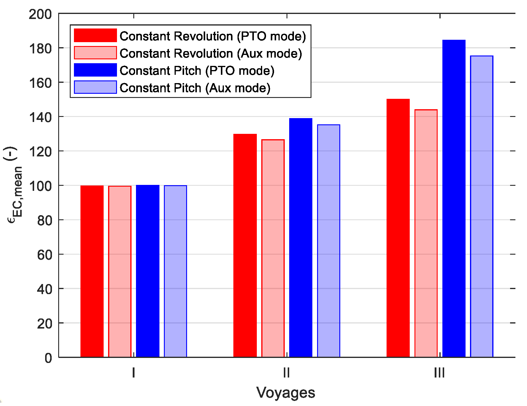
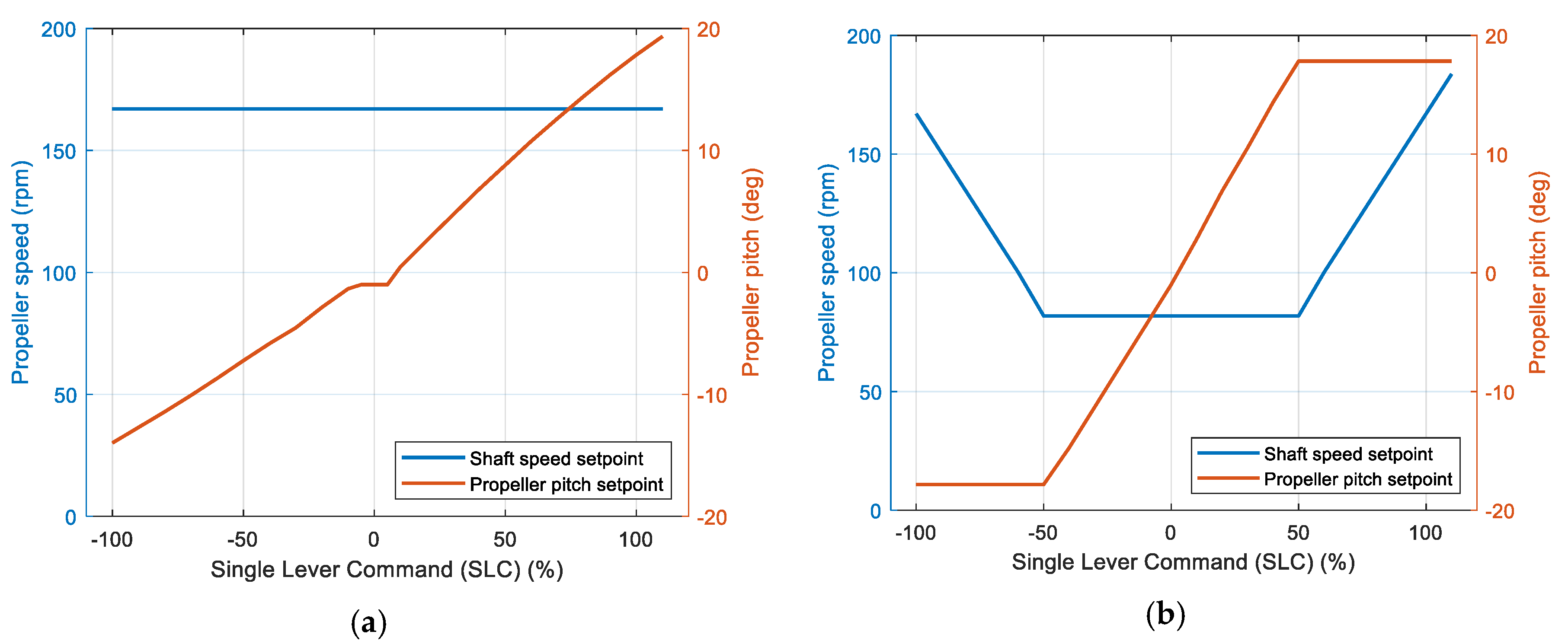
For each ship voyage, the influence of different ship propulsion control modes and electric power generation modes on the fuel consumption and emissions of the ship over the whole voyage will be investigated. The ship propulsion control modes (Constant Revolution Mode and Constant Pitch Mode) and electric power generation modes (PTO Mode and Aux Mode) have been introduced in [41] in details and they are briefly summarised in

Table 5. Ship propulsion control modes and power generating modes.

Propulsion Control Modes and Power Generating Modes		Descriptions
Propulsion control modes	Constant Revolution Mode	CONSTANT propeller revolution and CHANGING propeller pitch (Generator Law)
	Constant Pitch Mode	CONSTANT propeller pitch and CHANGING propeller revolution until minimum revolution is reached (Propeller Law)
Electric power generation modes	PTO Mode *	Shaft generator ON and auxiliary generator OFF
	Aux Mode	Shaft generator OFF and auxiliary generator ON

* PTO, power take off.

. The combinator curves for the two different propulsion control modes are shown in Figure A5 in Appendix C.

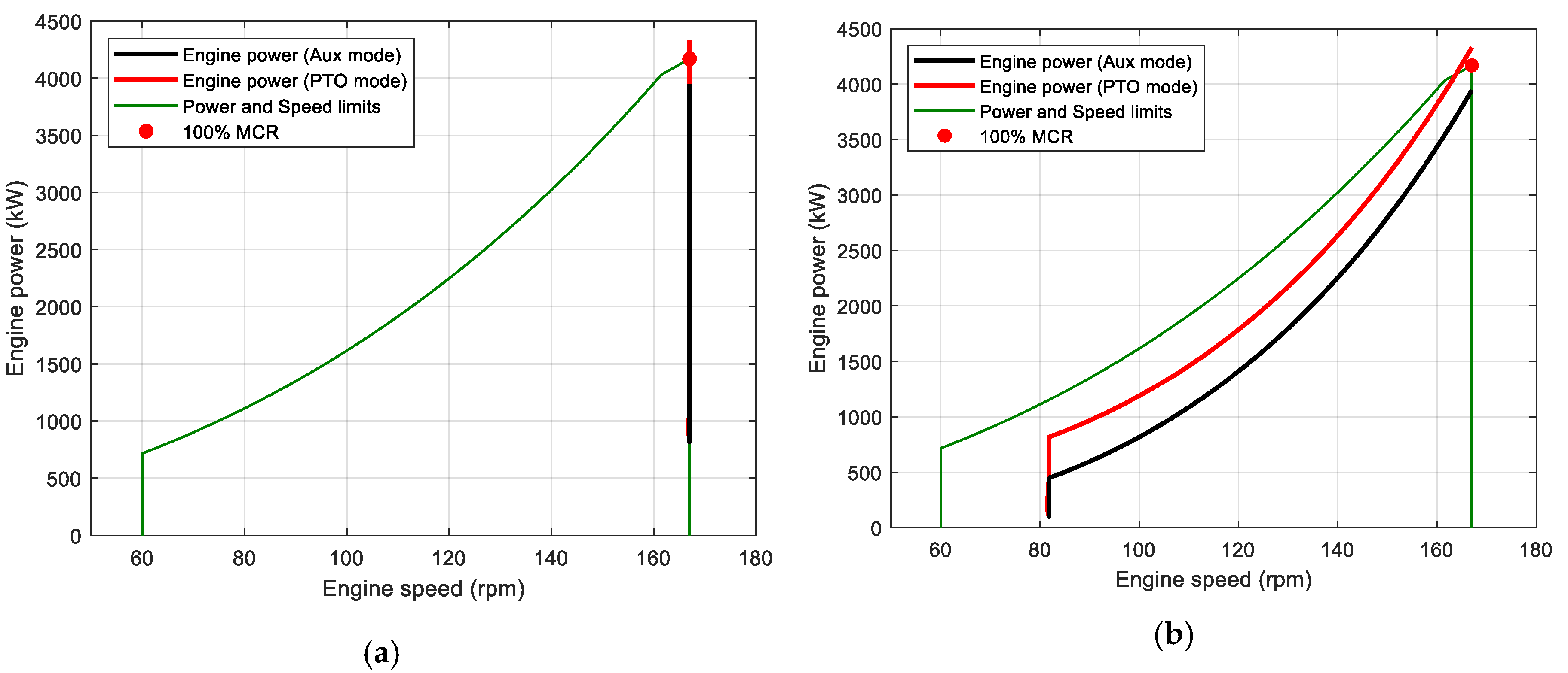
Note that, if the commanded ship speed cannot be reached within the power limit of the main engine because of providing PTO power, the shaft generator will be shut down and the electric power needed by the ship will be supplied by auxiliary generators, such as Transit A and Transit C of voyage I during which the PTO switch is turned off and the main engine only provides power for propulsion due to the demanded high ship speeds under the corresponding sea margin shown in Table 4.

5.2. Manoeuvring in Coastal and Port Areas

The ship mission profile during the close-to-port manoeuvre is shown in

Table 6. Ship mission profile sailing in coastal and port areas.

Sailing Area	Ship Mission Profile
Coastal Area	Ship Speed (kn)	7
	Sailing Distance (n mile)	40
	Sailing Time (h)	5.71
Port Area	Ship Speed (kn)	5
	Sailing Distance (n mile)	10
	Sailing Time (h)	2
The whole harbour approaching and leaving manoeuvre	Average speed (kn)	6.49
	Total Time (h)	7.71
	Total Distance (n mile)	50

. The ship speed is 7 knots in coastal areas and 5 knots in port areas. The sailing time and sailing distance of the ship in the same area are combined together, respectively, in the ship mission profile in Table 6. In coastal areas, the total sailing distance when approaching and leaving the harbour is 40 nautical miles and the total sailing time is 5.71 h. In port areas, the total sailing distance is 10 nautical miles and the total sailing time is 2 h. The sea margin when the ship is sailing in coastal and port areas is assumed to be normal, i.e., 15% sea margin, and the added ship resistance is because of the smaller depth in coastal and port areas compared with the open sea, where the sea state is the main reason for the added ship resistance.

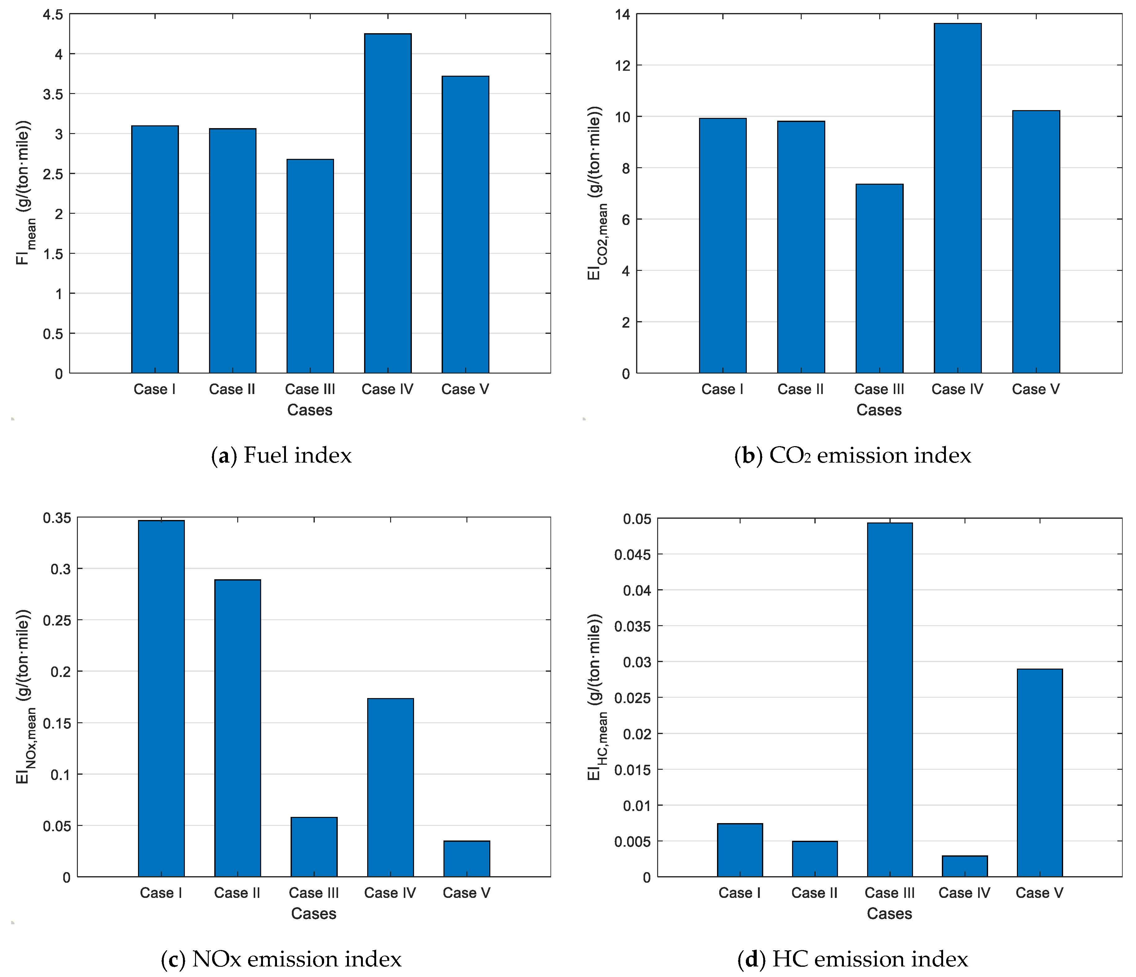
Five different operation cases of the ship are studied to investigate the influence of the ship propulsion and the electric generation modes of a hybrid propulsion ship on the fuel consumption and emissions performance during the close-to-port manoeuvre.

• In case I, the main engine burning heavy fuel oil (HFO) provides power for the ship propulsion and onboard electric loads through shaft generator in PTO mode, while the auxiliary engines are shut down.
• In case II, it is the same as case I except that the fuel burnt by the main engine is changed from heavy fuel oil (HFO) to marine diesel fuel (MDF).
• In case III, it is also the same as case I except that the fuel for the main engine is changed from HFO to LNG (liquefied natural gas).
• In case IV, the auxiliary engines burning marine diesel fuel (MDF) provide power for the ship propulsion through shaft motor in PTI mode and onboard electric loads, while the main engine is shut down.
• In case V, it is the same as case IV except that the fuel for the auxiliary engines is changed from MDF to LNG.

So, in case I, case II and case III, the ship propulsion system works in PTO mode but on different fuels; while in case IV and case V, the ship propulsion system works in PTI mode but on different fuels. Only the constant revolution mode, in which the ship speed is controlled by changing the propeller pitch and the propeller revolution is kept constant, will be studied during the close-to-port manoeuvre.

6. Results and Discussions

6.1. Average Ship Performance over Transit Voyage in Open Sea

6.1.1. Influence of Different Operation Modes

The influence of different propulsion control modes and electric power generation modes on the ship performance when sailing in the open sea has been investigated from the voyage perspective. In this section, the fuels for the main engine and the auxiliary engines are set as HFO and MDF, respectively. The average energy conversion effectiveness of the ship over the voyage is shown in Figure 3. In voyage I, where the average ship speed is 13.5 kn, different propulsion control and electric power generation modes do not make much difference on the average energy conversion effectiveness (around 100). The reason is that the propeller pitch of the two control modes is almost the same to reach that high ship speed. However, in voyage II and III, where the average ship speeds are 12 kn and 10 kn, respectively, the differences are much more obvious. The average energy conversion effectiveness will increase with the decrease in the average ship speed. Taking the constant revolution control and PTO electric generation modes, for example, the energy conversion effectiveness will increase from 100 to 130 and 150 when the average ship speed decreases from 13.5 kn (voyage I) to 12 kn (voyage II) and 10 kn (voyage III). The major reason is the increase in the ship weight/resistance ratio when reducing the ship speed and it is also the main reason why ship “slow steaming” can save fuel consumption over the voyage.

The “average” ship performance in terms of the fuel and emissions indices during the whole voyage of the ship are presented in Figure 4. The average fuel index (Figure 4a) and the average CO₂ emission index (Figure 4b) of the ship over the voyage are in fact the inverse of the average energy conversion effectiveness, so they have the inverse trends. For example, in constant pitch control mode and PTO electric generation mode, the fuel index will decrease from 4.37 to 3.15 and 2.37 (g/(ton·mile)), and the CO₂ emission index will decrease from 14.03 to 10.11 and 7.61 (g/(ton·mile)) when the average ship speed reduces from 13.5 to 12 and 10 (kn). Moreover, during the ship voyage, controlling the ship speed in constant pitch mode rather than the constant revolution mode, and providing the electric power by the shaft generator instead of the auxiliary generator will also reduce the fuel consumption and CO₂ emission over the voyage.

When the average ship speed decreases, the average NOx and HC emission index over the whole voyage will also reduce as shown in Figure 4c,d. For instance, under constant pitch and PTO electric generation mode, the NOx emission index decreases from 0.33 to 0.24 and 0.17 (g/(ton·mile)) and the HC index reduces from 0.0118 to 0.0098 and 0.0081 (g/(ton·mile)). The constant pitch mode has a higher average NOx emission index (Figure 4c) than the constant revolution mode. Generating the electric power in PTO mode during the ship voyage will also reduce the NOx emission especially in constant pitch operating mode. The constant revolution mode has lower HC emission index (Figure 4d) than the constant pitch mode especially at low average ship speeds. Unlike the average fuel consumption, CO₂ emission and NOx emission, the average HC emission over the voyage will increase when the electric power is provided by the shaft generator (PTO mode). According to the simulation results of the defined three voyages, an efficient way to reduce the fuel consumption and emissions indexes is to reduce the average ship speed of the voyage, i.e., slow steaming. Different propulsion control modes and power generation modes also make some differences on the average fuel consumption and emissions indexes of the voyage especially at low ship speeds.

6.1.2. Influence of Sailing on Different Fuels

In this section, when investigating the influence of different fuel types on the fuel consumption and emissions over the whole transit voyage, only voyage II, in which the ship sails at 12 knots while at sea, will be looked into. The propulsion control mode is set as constant pitch mode and the electric generation mode is set as PTO mode. The average fuel and emissions indices of the ship over the whole transit voyage when sailing on different fuels, i.e., HFO, MDF and LNG, are shown in Figure 5. The average fuel index of the ship (Figure 5a) when sailing on LNG (2.727 g/(ton·mile)) is about 13.5% less compared with sailing on HFO (3.154 g/(ton·mile)) and 12.5% less than MDF (3.117 g/(ton·mile)). The average CO₂ emission index of the ship (Figure 5b) when sailing on LNG (7.50 g/(ton·mile)) is about 25.8% less compared with sailing on HFO (10.11 g/(ton·mile)) and 25% less than MDF (10.00 g/(ton·mile)). Note that, the lower heat values (LHV) and the conversion factors between fuel consumption and CO₂ emissions are different for different fuels. The average NOx emission index of the ship (Figure 5c) when sailing on MDF (0.196 g/(ton·mile)) is about 17% less than sailing on HFO (0.236 g/(ton·mile)), while sailing on LNG (0.039 g/(ton·mile)) can further reduce the NOx emission index by 80% compared with sailing on MDF. However, the average HC emission index (Figure 5d) of the ship when sailing on LNG (0.065 g/(ton·mile)) is much higher than sailing on HFO (0.0098 g/(ton·mile)) and MDF (0.0065 g/(ton·mile)), which is one of the major disadvantages of using LNG as the marine fuel. This is primarily caused by methane slip and unburnt methane during engine operations.

6.2. Average Ship Performance over Manoeuvring in Close-to-Port Areas

The fuel consumption and emissions performance of the ship during manoeuvre in close-to-port areas under five different operation cases introduced in Section 5.2 are investigated. The fuel consumption and emissions of the ship during the whole close-to-port manoeuvre are shown in Figure 6. The average fuel indices (Figure 6a) and CO₂ emission indices (Figure 6b) of the ship when sailing on main engine in PTO mode (Case I, II and III) are lower than sailing on auxiliary engines in PTI mode (Case IV and V). However, sailing on auxiliary engines in PTI mode can reduce the local NOx (Figure 6c) and HC emissions indices (Figure 6d) significantly compared with sailing on the main engine in PTO mode.

When sailing on conventional fuels (Case I, II and IV), the fuel index and CO₂ emission index in case I, which are 3.10 and 9.93 (g/(ton·mile)), respectively, are slightly higher than those in Case II, which are 3.06 and 9.81 (g/(ton·mile)); but they are notably lower than those in Case IV, which are 4.25 and 13.62 (g/(ton·mile)), respectively. However, the NOx and HC emission indices in Case I, which are 0.35 and 0.0074 (g/(ton·mile)), respectively, are much higher than those in Case II, which are 0.28 and 0.0049 (g/(ton·mile)), respectively; the NOx and HC emission indices in Case IV, which are 0.17 and 0.0029 (g/(ton·mile)), respectively, are further lower than Case II. The reason is that the fuel consumption performance of the main engine (two-stroke) is better than that of the auxiliary engine (four-stroke) burning MDF while the NOx and HC emission performance of the main engine is worse especially when burning HFO compared with the auxiliary engine.

Sailing on LNG (Case III and V) instead of conventional fuels in coastal and port areas can both reduce fuel consumption and CO₂ emission indices of the ship, in particular the local NOx emission index (0.058 g/(ton·mile) in Case III and 0.035 g/(ton·mile) in Case V) will decrease significantly. However, the local HC emission index (0.049 g/(ton·mile) in Case III and 0.029 g/(ton·mile) in Case V) is much higher when sailing on LNG than sailing on HFO and MDF.

Therefore, comparing the five cases, in order to reduce the ship emissions significantly when manoeuvring in close-to-port areas, the ship should be driven by the auxiliary engines through PTI mode. However, a balance between CO₂ and NOx emissions on the one hand and HC emissions on the other needs to be made when selecting to sail the ship on LNG rather than the conventional fuels. Note that, as mentioned earlier, the methane emissions of LNG have no direct health effects on humans. At the same time, it is actually a more potent greenhouse gas than CO₂. So, reducing the local pollution point of view when driving the ship in PTI mode and LNG fuel when manoeuvring in close-to-port areas are better choices compared to the other cases.

6.3. Fuel Consumption and Emissions of the Whole Voyage

In summary, the average fuel and emissions indexes of the ship over the whole voyage, including transit at open sea, approaching and leaving harbour manoeuvre, are shown in

Table 7. Average fuel and emissions indexes of the whole voyage.

Fuel Type	HFO	LNG
$\overline{FI}$ (g/(ton·mile))	3.15	2.72
${\overline{EI}}_{CO2}$ (g/(ton·mile))	10.10	7.49
${\overline{EI}}_{NOx}$ (g/(ton·mile))	0.24	0.041
${\overline{EI}}_{HC}$ (g/(ton·mile))	0.0096	0.0642

. According to the previous discussions in Section 6.1 and Section 6.2, there are many different combinations of ship operation cases during the whole voyage. For simplicity, only two cases sailing the ship on two different fuels, i.e., HFO and LNG, have been selected and are shown in Table 7. The propulsion control modes for transit in open sea and manoeuvring in close-to-port areas are set as constant pitch mode and constant revolution mode, respectively; the electric power generation modes for the whole voyage are set as PTO mode. Compared to transit in open sea, harbour approaching and leaving manoeuvres only take a small part of the total voyage, so, the results of the total voyage shown in Table 7 are mainly determined by the fuel and emissions indexes of the voyage when sailing at open sea.

7. Conclusions and Recommendations

In this paper, the influences of the ship propulsion control modes, electric power generation modes, ship operational speeds, propulsion modes as well as sailing on different fuels on the fuel consumption and emissions of an ocean-going benchmark chemical tanker have been investigated taking the ship’s operational profiles into account. The current IMO’s EEDI considers only one operating point when estimating ship energy efficiency, however, a lower EEDI does not necessarily mean less ship fuel consumption and emissions when sailing with a certain mission profile over the whole voyage. So, the mean value indicators weighted over the ship mission profile should be used when estimating the fuel consumption and emissions performance of the ship over the voyage.

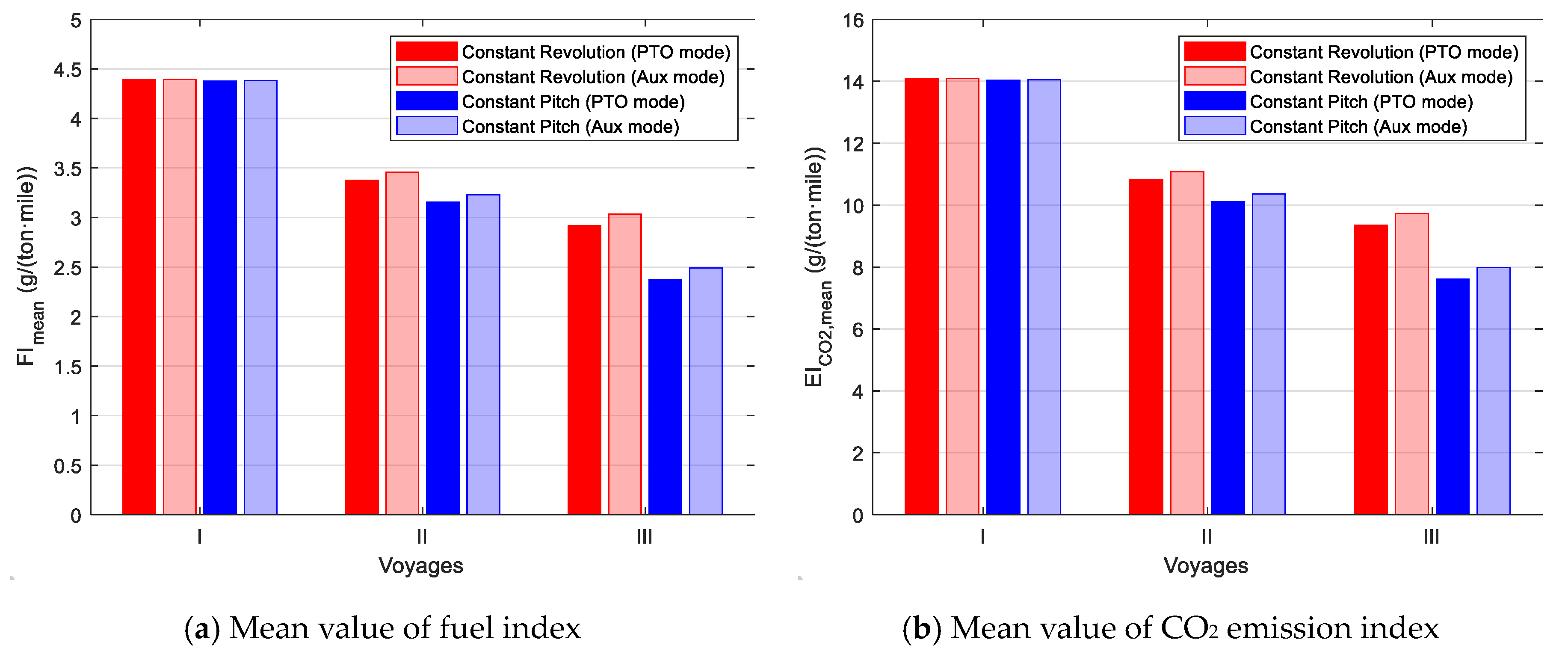
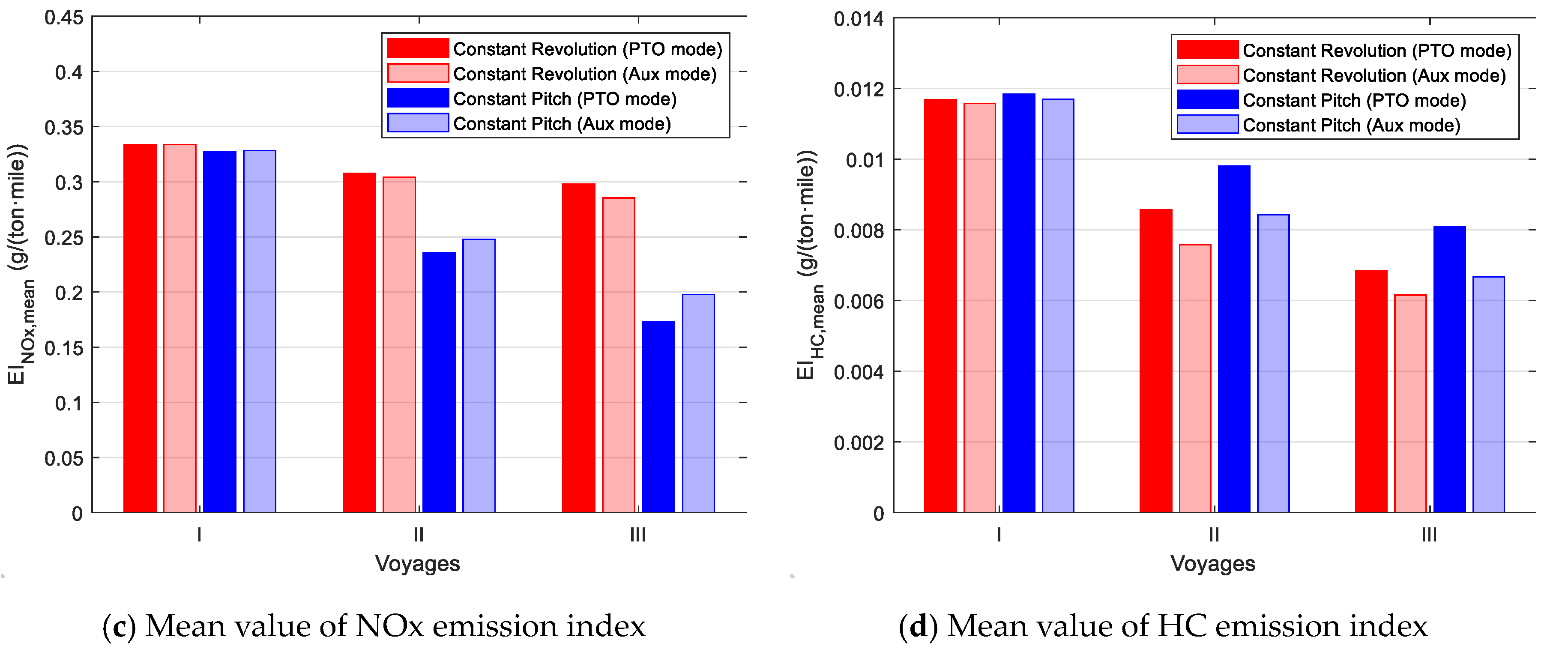
When transiting in open sea, reducing the ship average operational speed will effectively reduce both the fuel consumption and emissions of the ship over the voyage. To reduce the ship operational speed, reducing the propeller revolution rather than the propeller pitch is more preferable, as pitch reduction will reduce the propeller efficiency and consequently increase the fuel consumption especially for voyage where the ship speed is reduced. Generating the electric power by the shaft generator (PTO mode) rather than the auxiliary generator (Aux mode) will further reduce the fuel consumption while the NOx and HC emissions could increase. However, compared to the propulsion control modes, the electric generation modes have relatively minor influence on fuel consumption and emissions of the ship.

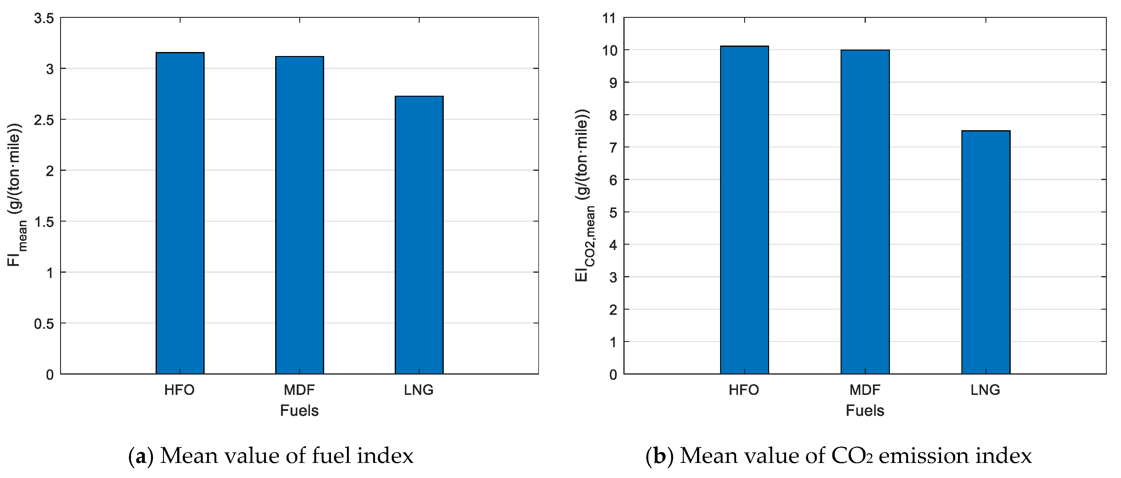
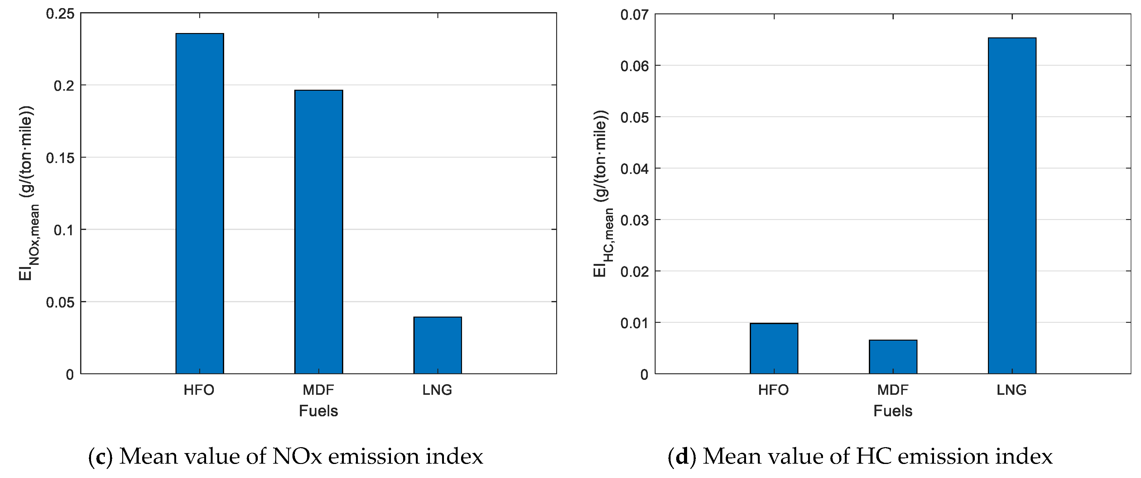
When the ship is sailing and manoeuvring in the coastal and port areas, changing the fuel for the main engine from heavy fuel oil (HFO) to marine diesel fuel (MDF) will reduce the NOx and HC emissions significantly while slightly reducing the fuel consumption and CO₂ emissions. Providing the power for ship propulsion (PTI mode) and onboard electric loads by the auxiliary engines and shutting down the main engine will further reduce the local NOx and HC emissions significantly while the fuel consumption and CO₂ emission will increase notably mainly due to the lower engine efficiency of the auxiliary engines.

Using LNG (liquefied natural gas) as the fuel for both the main and auxiliary engines will reduce the NOx emission significantly compared to using HFO (heavy fuel oil) or MDF (marine diesel fuel). So, sailing the ship on LNG in close-to-port areas will produce much less local environmental impact due to the much less local pollutant emissions. In particular, sailing the ship in PTI mode on LNG will further reduce the local pollutant emissions in coastal and port areas. The fuel consumption and CO₂ emission of the ship will also decrease notably over the whole voyage when sailing on LNG instead of HFO and MDF. However, the hydrocarbon (HC) emission is much higher when using LNG as a marine fuel than traditional diesel fuel due to the methane (CH₄) slip and unburnt methane during engine operations and although it has no direct effects on human health, it may have a worse impact on climate change (global warming) when taking the life-cycle emissions of natural gas into consideration (although the lifetime of the emitted substance should then also be taken into account, which is outside the scope of this paper). It is clear either way that methane emissions from LNG engines should be minimised as much as possible.

Last but not least, there are still some limitations and uncertainties existing in this paper and these will be further studied in future work. One of the limitations is that only CO₂, NOx and HC emissions are investigated and the other emissions, such as sulphur oxides (SOx), particulate matter (PM) and soot (C), etc., generated by the ship are not considered. Another limitation is that only fuel consumption and emissions are investigated in this paper while the ship capital expenditure (CAPEX), operating expenditure (OPEX) and the operational safety of both the engine and ship have been left outside the scope. The uncertainty is in the simplistic assumption on the fuel consumption and emission performance of the engines when using LNG as the fuel. In future work, in addition to improving the fuel consumption and emissions models, the potential influence of the application of the hybrid propulsion and alternative fuels on the CAPEX and OPEX of the ship, and the operational safety of both the engine and ship especially in adverse sea conditions will be investigated. The trade-off relationships between the ship CAPEX and OPEX, and between the energy effectiveness of the ship and the operational safety, need to be investigated.

References

1. Chapman, L. Transport and climate change: A review. J. Transp. Geogr. 2007, 15, 354–367. [Google Scholar] [CrossRef]
2. UNCTAD. Review of Maritime Transport 2019; UNITED Nations Publication: Geneva, Switzerland, 2019. [Google Scholar]
3. Shi, W. Dynamics of Energy System Behaviour and Emissions of Trailing Suction Hopper Dredgers. Ph.D. Thesis, Delft University of Technology, Delft, The Netherlands, 2013. [Google Scholar]
4. Moreno-Gutiérrez, J.; Pájaro-Velázquez, E.; Amado-Sánchez, Y.; Rodríguez-Moreno, R.; Calderay-Cayetano, F.; Durán-Grados, V. Comparative analysis between different methods for calculating on-board ship’s emissions and energy consumption based on operational data. Sci. Total Environ. 2019, 650, 575–584. [Google Scholar] [CrossRef]
5. Taljegard, M.; Brynolf, S.; Grahn, M.; Andersson, K.; Johnson, H. Cost-effective choices of marine fuels in a carbon-constrained world: Results from a global energy model. Environ. Sci. Technol. 2014, 48, 12986–12993. [Google Scholar] [CrossRef]
6. IMO. Third IMO Greenhouse Gas Study 2014, Executive Summary and Final Report; International Maritime Organisation (IMO): London, UK, 2015. [Google Scholar]
7. Perera, L.P.; Mo, B.; Kristjánsson, L.A.; Jønvik, P.C.; Svardal, J.Ø. Evaluations on ship performance under varying operational conditions. In Proceedings of the 34th International Conference on Ocean, Offshore and Arctic Engineering, St. John’s, NL, Canada, 31 May–5 June 2015. [Google Scholar]
8. Andersson, K.; Baldi, F.; Brynolf, S.; Lindgren, J.F.; Granhag, L.; Svensson, E. Shipping and the Environment; Springer: Berlin/Heidelberg, Germany, 2016; pp. 3–27. [Google Scholar]
9. Klein Woud, H.; Stapersma, D. Design of Propulsion and Electric Power Generation Systems; IMarEST, Institute of Marine Engineering, Science and Technology: London, UK, 2002. [Google Scholar]
10. Stapersma, D. Main Propulsion Arrangement and Power Generation Concepts. Encyclopedia of Maritime and Offshore Engineering; John Wiley & Sons, Ltd.: Hoboken, NJ, USA, 2017; pp. 1–40. [Google Scholar]
11. MEPC. Guidelines for voluntary use of the ship energy efficiency operational indicator (EEOI). In International Maritime Organization Report; MEPC.1/Circ.684, 17 August 2009; IMO: London, UK, 2009. [Google Scholar]
12. Acomi, N.; Acomi, O.C. Improving the Voyage Energy Efficiency by Using EEOI. Procedia-Soc. Behav. Sci. 2014, 138, 531–536. [Google Scholar] [CrossRef] [Green Version]
13. Coraddu, A.; Figari, M.; Savio, S. Numerical investigation on ship energy efficiency by Monte Carlo simulation. Proc. Inst. Mech. Eng. Part M J. Eng. Marit. Environ. 2014, 228, 220–234. [Google Scholar] [CrossRef]
14. Hou, Y.H.; Kang, K.; Liang, X. Vessel speed optimization for minimum EEOI in ice zone considering uncertainty. Ocean Eng. 2019, 188, 106240. [Google Scholar] [CrossRef]
15. Safaei, A.; Ghassemi, H.; Ghiasi, M. Voyage Optimization for a Very Large Crude Carrier Oil Tanker: A Regional Voyage Case Study. Sci. J. Marit. Univ. Szczec. 2015, 44, 83–89. [Google Scholar]
16. Zaccone, R.; Ottaviani, E.; Figari, M.; Altosole, M. Ship voyage optimization for safe and energy-efficient navigation: A dynamic programming approach. Ocean Eng. 2018, 153, 215–224. [Google Scholar] [CrossRef]
17. Geertsma, R.D.; Negenborn, R.R.; Visser, K.; Loonstijn, M.A.; Hopman, J.J. Pitch control for ships with diesel mechanical and hybrid propulsion: Modelling, validation and performance quantification. Appl. Energ. 2017, 206, 1609–1631. [Google Scholar] [CrossRef]
18. Geertsma, R.D.; Visser, K.; Negenborn, R.R. Adaptive pitch control for ships with diesel mechanical and hybrid propulsion. Appl. Energy 2018, 228, 2490–2509. [Google Scholar] [CrossRef]
19. Kalikatzarakis, M.; Geertsma, R.D.; Boonen, E.J.; Visser, K.; Negenborn, R.R. Ship energy management for hybrid propulsion and power supply with shore charging. Control Eng. Pract. 2018, 76, 133–154. [Google Scholar] [CrossRef]
20. Vu, T.L.; Ayu, A.A.; Dhupia, J.S.; Kennedy, L.; Adnanes, A.K. Power Management for Electric Tugboats Through Operating Load Estimation. IEEE Trans. Control Syst. Technol. 2015, 23, 2375–2382. [Google Scholar] [CrossRef]
21. Zhao, F.; Yang, W.; Tan, W.W.; Yu, W.; Yang, J.; Chou, S.K. Power management of vessel propulsion system for thrust efficiency and emissions mitigation. Appl. Energy 2016, 161, 124–132. [Google Scholar] [CrossRef]
22. Psaraftis, H.N.; Kontovas, C.A. Speed models for energy-efficient maritime transportation: A taxonomy and survey. Transp. Res. Part C Emerg. Technol. 2013, 26, 331–351. [Google Scholar] [CrossRef]
23. Lee, C.; Lee, H.L.; Zhang, J. The impact of slow ocean steaming on delivery reliability and fuel consumption. Transp. Res. Part E Logist. Transp. Rev. 2015, 76, 176–190. [Google Scholar] [CrossRef]
24. Carlton, J.; Aldwinkle, J.; Anderson, J. Future ship powering options: Exploring alternative methods of ship propulsion. Lond. R. Acad. Eng. 2013, 2013, 1–95. [Google Scholar]
25. Bouman, E.A.; Lindstad, E.; Rialland, A.I.; Strømman, A.H. State-of-the-art technologies, measures, and potential for reducing GHG emissions from shipping—A review. Transp. Res. Part D Transp. Environ. 2017, 52, 408–421. [Google Scholar] [CrossRef]
26. Geertsma, R.D.; Negenborn, R.R.; Visser, K.; Hopman, J.J. Design and control of hybrid power and propulsion systems for smart ships: A review of developments. Appl. Energy 2017, 194, 30–54. [Google Scholar] [CrossRef]
27. Kwasieckyj, B. Efficiency Analysis and Design Methodology of Hybrid Propulsion Systems. Master’s Thesis, Delft University of Technology, Delft, The Netherlands, 2013. [Google Scholar]
28. Bennabi, N.; Charpentier, J.F.; Menana, H.; Billard, J.Y.; Genet, P. Hybrid propulsion systems for small ships: Context and challenges. In Proceedings of the 2016 XXII International Conference on Electrical Machines (ICEM), Lausanne, Switzerland, 4–7 September 2016; pp. 2948–2954. [Google Scholar]
29. Jafarzadeh, S.; Schjølberg, I. Operational profiles of ships in Norwegian waters: An activity-based approach to assess the benefits of hybrid and electric propulsion. Transp. Res. Part D Transp. Environ. 2018, 65, 500–523. [Google Scholar] [CrossRef] [Green Version]
30. Yum, K.K.; Skjong, S.; Tasker, B.; Pedersen, E.; Steen, S. Simulation of a Hybrid Marine Propulsion System in Waves. In Proceedings of the 28th CIMAC World Congress, Helsinki, Finland, 6–10 June 2016. [Google Scholar]
31. Dedes, E.K.; Hudson, D.A.; Turnock, S.R. Investigation of Diesel Hybrid systems for fuel oil reduction in slow speed ocean going ships. Energy 2016, 114, 444–456. [Google Scholar] [CrossRef] [Green Version]
32. Kern, C.; Tvete, H.A.; Alnes, Ø.Å.; Sletten, T.; Hansen, K.R.; Knaf, A.; Sames, P.; Puchalski, S. Battery Hybrid Oceangoing Cargo Ships. In Proceedings of the CIMAC Congress 2019, Vancouver, BC, Canada, 10–14 June 2019. [Google Scholar]
33. Sui, C.; Stapersma, D.; Visser, K.; Ding, Y.; de Vos, P. Impact of Battery-Hybrid Cargo Ship Propulsion on Fuel Consumption and Emissions during Port Approaches. In Proceedings of the CIMAC Congress 2019, Vancouver, BC, Canada, 10–14 June 2019. [Google Scholar]
34. Wei, L.; Geng, P. A review on natural gas/diesel dual fuel combustion, emissions and performance. Fuel Process Technol. 2016, 142, 264–278. [Google Scholar] [CrossRef]
35. Brynolf, S.; Fridell, E.; Andersson, K. Environmental assessment of marine fuels: Liquefied natural gas, liquefied biogas, methanol and bio-methanol. J. Clean Prod. 2014, 74, 86–95. [Google Scholar] [CrossRef]
36. Burel, F.; Taccani, R.; Zuliani, N. Improving sustainability of maritime transport through utilization of Liquefied Natural Gas (LNG) for propulsion. Energy 2013, 57, 412–420. [Google Scholar] [CrossRef]
37. Thomson, H.; Corbett, J.J.; Winebrake, J.J. Natural gas as a marine fuel. Energy Policy 2015, 87, 153–167. [Google Scholar] [CrossRef] [Green Version]
38. Acciaro, M. Real option analysis for environmental compliance: LNG and emission control areas. Transp. Res. Part D Transp. Environ. 2014, 28, 41–50. [Google Scholar] [CrossRef]
39. Schinas, O.; Butler, M. Feasibility and commercial considerations of LNG-fueled ships. Ocean Eng. 2016, 122, 84–96. [Google Scholar] [CrossRef]
40. AEsoy, V.; Einang, P.M.; Stenersen, D.; Hennie, E.; Valberg, I. LNG-fuelled engines and fuel systems for medium-speed engines in maritime applications. SAE Tech. Pap. 2011. [Google Scholar] [CrossRef]
41. Sui, C.; Stapersma, D.; Visser, K.; de Vos, P.; Ding, Y. Energy effectiveness of ocean-going cargo ship under various operating conditions. Ocean Eng. 2019, 190, 106473. [Google Scholar] [CrossRef]
42. Lehtoranta, K.; Aakko-Saksa, P.; Murtonen, T.; Vesala, H.; Kuittinen, N.; Rönkkö, T.; Ntziachristos, L.; Karjalainen, P.; Timonen, H.; Teinilä, K. Particle and Gaseous Emissions from Marine Engines Utilizing Various Fuels and Aftertreatment Systems. In Proceedings of the CIMAC Congress 2019, Vancouver, BC, Canada, 10–14 June 2019. [Google Scholar]
43. Anderson, M.; Salo, K.; Fridell, E. Particle- and Gaseous Emissions from an LNG Powered Ship. Environ. Sci. Technol. 2015, 49, 12568–12575. [Google Scholar] [CrossRef]
44. Stapersma, D. Diesel Engines—A Fundamental Approach to Performance Analysis, Turbocharging, Combustion, Emissions and Heat Transfer. In Emissions and Heat Transfer, Part II: Diesel Engines B—Combustion, Emissions and Heat Transfer; Lecture Notes NLDA/TUDelft April 2010; NLDA & Delft UT: Delft, The Netherlands, 2010. [Google Scholar]
45. Jo, J.Y.; Kwon, Y.S.; Lee, J.W.; Park, J.S.; Rho, B.H.; Choi, W. Acute respiratory distress due to methane inhalation. Tuberc. Respir. Dis. 2013, 74, 120–123. [Google Scholar] [CrossRef] [Green Version]
46. IMO. Annex 5 Resolution Mepc.308(73) (Adopted on 26 October 2018) 2018 Guidelines on the Method of Calculation of the Attained Energy Efficiency Design Index (eedi) for New Ships; IMO: London, UK, 2018. [Google Scholar]
Figure 1. Layout of the updated chemical tanker propulsion system and electric generating system.
Jmse 08 00588 g001
Figure 2. Model structure of the integrated ship propulsion and electric generation systems.
Jmse 08 00588 g002
Figure 3. Mean value of energy conversion effectiveness.
Jmse 08 00588 g003
Figure 4. Mean value of fuel and emissions indices.
Jmse 08 00588 g004aJmse 08 00588 g004b
Figure 5. Mean value of fuel and emissions indices when using different fuels.
Jmse 08 00588 g005aJmse 08 00588 g005b
Figure 6. Fuel and emissions indices in different cases.
Jmse 08 00588 g006