4.1.1. Grid Convergence Test
Four different computational grids consisting of 8.27, 15.98, 31.09 and 63.48 million cells respectively, are considered in the following to host the grid convergence test computations. Let these grids be denoted by coarse, medium, fine and very fine for the convenience of a proper identification of each computational case. The thrust and torque coefficients are computed for a series of eight advance ratios ranging from 0.6418 to 1.6563 and compared with the corresponding experimental data [
36], as tabulated in
Table 3 and
Table 4. In all computations the rate of revolution is kept constant at a value of 600 rpm, whereas the inflow speed corrected at experiments with idle torque and gap force is varied to achieve the different advance ratios.
For the sake of consistency, all the computations employ the DES turbulence model and all the reported solutions are computed for 25 s physical time when the propeller has already performed 250 complete rotations. All the parallel computations are performed on 120 processors, which means that for the finest grid case, a number of about 529,000 cells are computed on each processor.
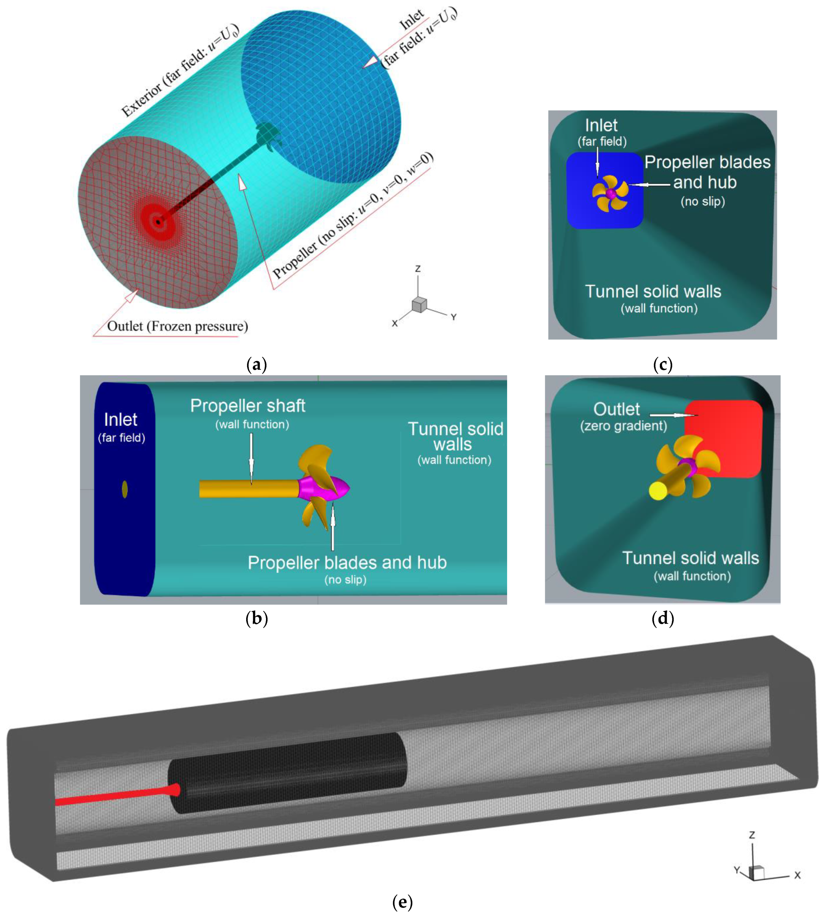
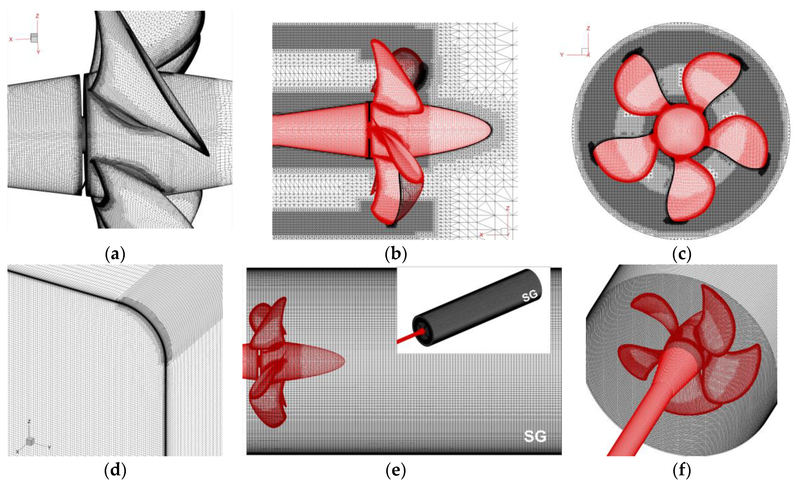
Automatic mesh refinement is performed based on sensors placed next to solid walls and inside the wake. Special attention to the quality criteria such as orthogonality, smoothness and clustering inside the areas next to the solid boundaries is paid during the generation process. Areas of rather heavy clustering are placed around the blade edges and tips and hub and shaft, as depicted in
Figure 2. Aside from that, an annular volume of grid refinement is generated in the wake of the propeller, therefore in the region where large gradients of the flow parameters are expected to occur. In the immediate proximity of the propeller, the grid lines perpendicular to the wall are refined substantially to maintain a
value less than unity for the first layer of grid cells.
All the computations are performed on a high-performance computer with 624 Intel E5 2680 v3 processors with 12 cores with a frequency of 2.5 GHz and 3.3 GHz for the turbo boost regime. In the very fine mesh computational case, an average of 0.205 millisecond per mesh point was necessary. As said before, each simulation is performed for 25 s, out of which the rotational acceleration time done on a half sinusoidal law is imposed for two seconds. A time of 15 to 17 s is sufficient to achieve the convergence of both thrust and torque computed coefficients.
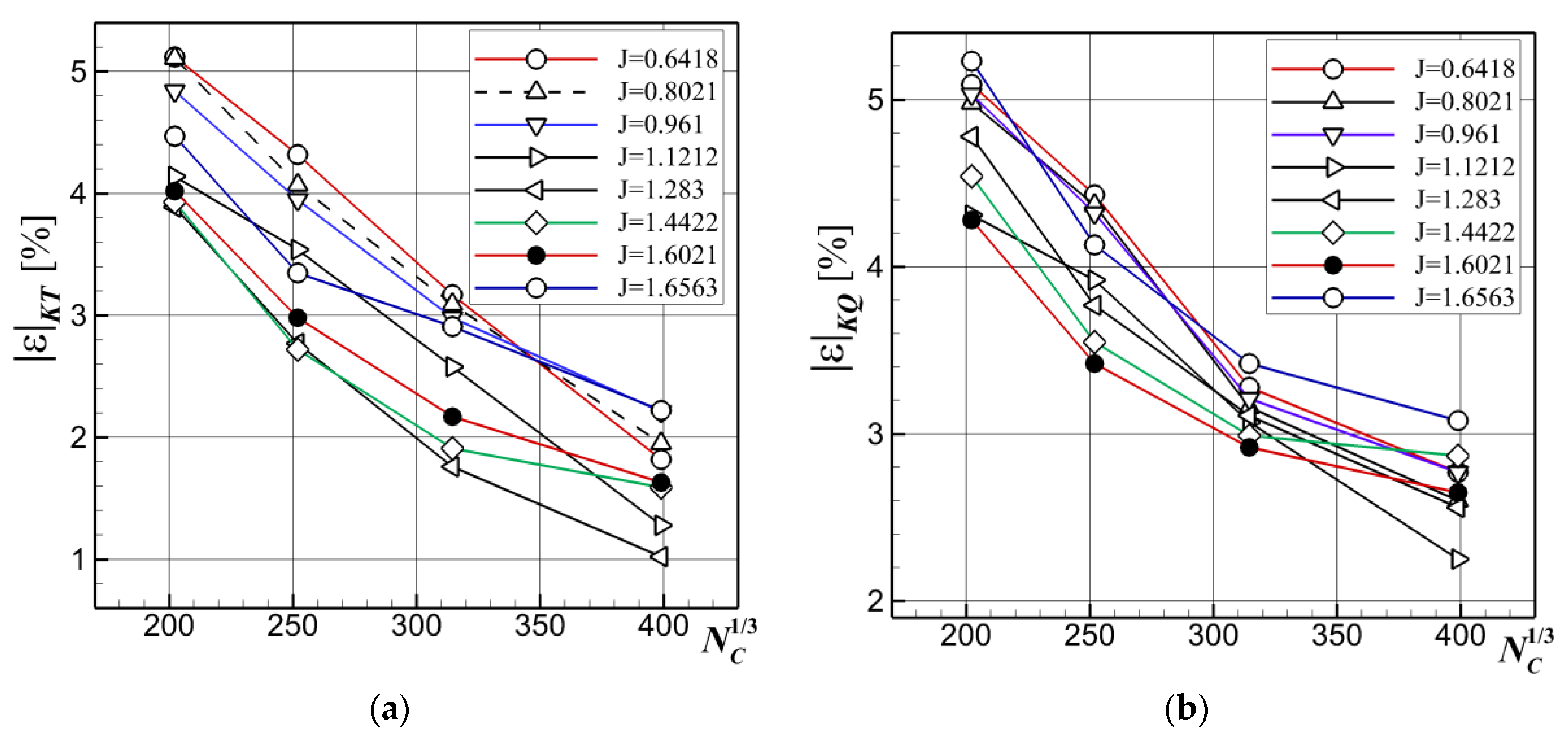
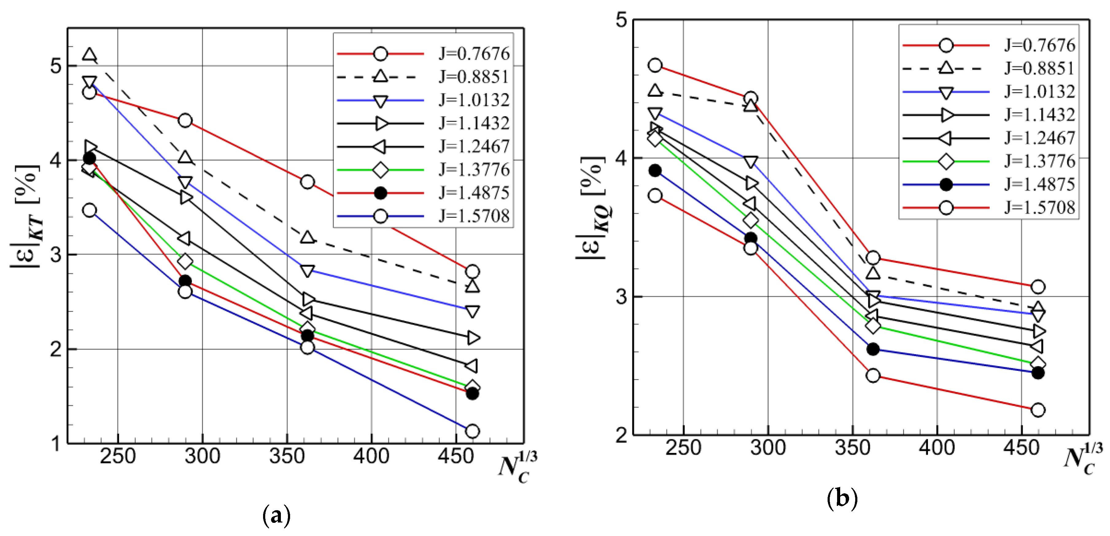
The variation of the computed errors of the numerical solutions compared to the experimental data [
36] is depicted in
Figure 3a for the thrust coefficient and
Figure 3b for the torque coefficient. The reason for reporting the solutions in the abscissae to the cubic root of the number of cells of a given computation is that when using an unstructured grid it is difficult to define another relevant parameter to describe locally the grid resolution.
Obviously, the general trend of the solutions shows that with the increase of the accuracy of the discretization, the errors are monotonically decreasing, a fact that is sustained by the theory of numerics. Nevertheless, there are some advance coefficients for which variation slope does not wholly sustain the above statement, a fact which is not generally in conflict with the general rule of the monotonic decrease of the computational error with the increase of the discretization accuracy. As an overall conclusion based on
Figure 3, the reader may notice that the grid convergence test sustains not only the consistency of the numerical model used in the present study, but also the robustness of the solver.
The grid uncertainty is further evaluated by following the methodology described in [
37] for monotonic convergence. The verification and validation will be carried out only for the
J=1.283 case, which produced the smallest error of the thrust coefficient compared to the experimental data. Let the four meshes considered in the grid convergence computations be denoted by
M1…
M4, where
M1 corresponds to the coarse mesh and
M4 to the very fine one. The grid ratio (
rG), the associated relative error between the
KT computed on the very fine mesh
M4 and the fine mesh
M3,
, the ratio between the estimated order of convergence and the theoretical order of convergence,
pG/
pGth, the grid uncertainty,
UG%M4, the experimental uncertainty,
UD%D, and the validation uncertainty,
Uv%, are tabulated in
Table 5.
pG,th in
Table 5 is the theoretical order of accuracy, which is the order of convection scheme, whereas the validation uncertainty is
. The relative error between the solution computed on the finest mesh
M4 and the experimental data for the thrust coefficient is smaller than the Richardson-based validation numerical uncertainty, therefore the
KT prediction can be considered as being validated. A similar conclusion can be withdrawn for
KQ.
4.1.2. Propeller Performances and Flow Analysis
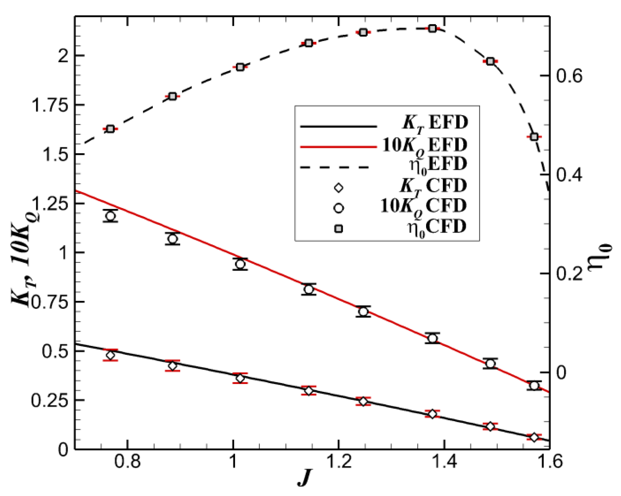
Having carried out the grid convergence test, in the following only the solutions computed on the very fine grid will be reported and discussed. Prediction of thrust and torque realized by the propeller is performed first. The computed propeller performance coefficients are tabulated in
Table 6 for all the advance ratios and compared with the corresponding experimental data reported in [
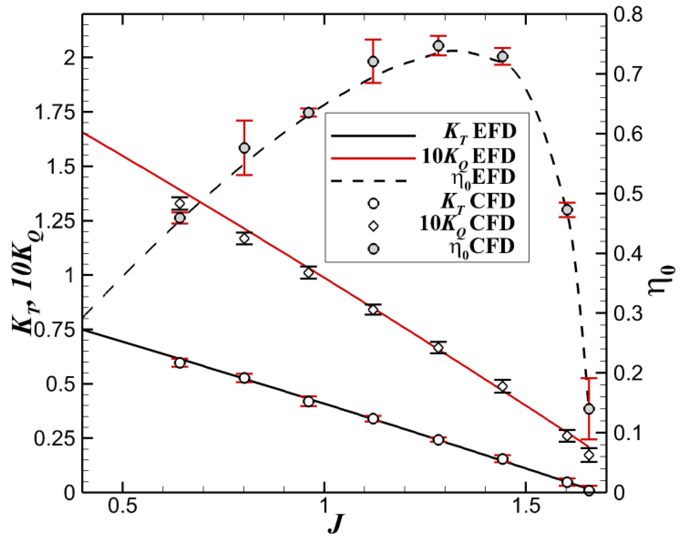
36]. The level of errors is limited to 2.22% for the thrust coefficient and to 3.08% for the torque coefficient. A slight underestimation of the thrust may be seen for almost all the advance ratios. In spite of that fact, it is worth mentioning that the computed and experimental curves almost overlap and their slopes are practically coincident, as depicted in
Figure 4. Things are rather similar for the torque coefficient, although the level of the errors is slightly higher. Seemingly, the reason behind the differences is related to the small values of the torque, a fact that sometimes brings numerical difficulties, although all the computations reported here were performed in double precision. The highest level of errors for the open water efficiency coefficients reaches a value slightly larger than 5% for the highest advance ratio, at which the thrust and torque have the lowest values over the domain, as
Figure 4 bears out.
The numerical solutions reported here are very similar to those reported in [
38], even though the solvers were different and the closure to turbulence was achieved by using different models. Moreover, the present solutions are in a good agreement with most of those reported in [
39], where various solvers were used to solve the benchmark case of the PPTC propeller by 14 attendees of the symposium. That is, the same trend was noticed in the concluding remarks of the final report of the symposium, which noticed that the numerical solutions reported by most of the participants slightly underestimated the thrust and torque coefficients as well.
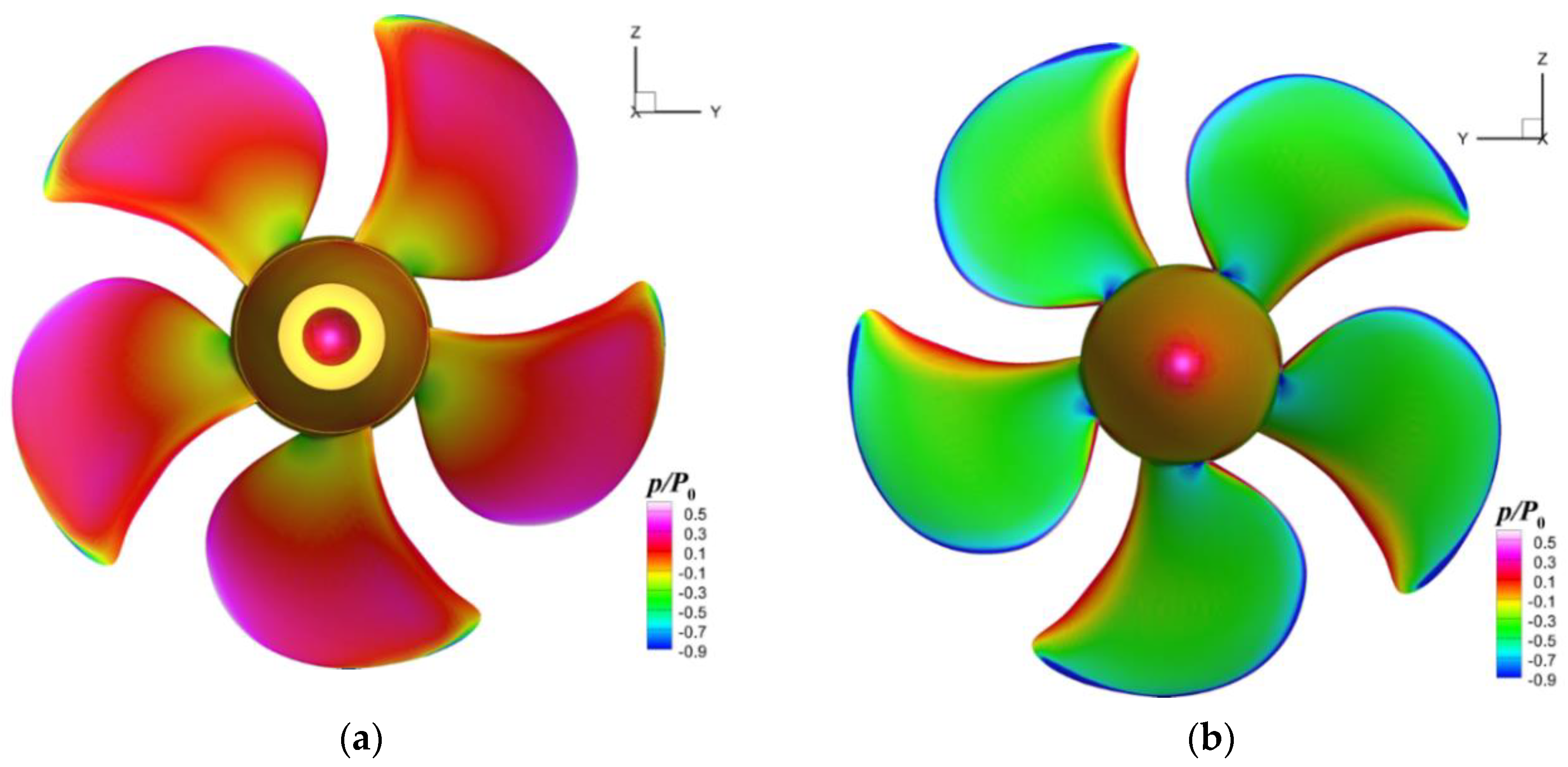
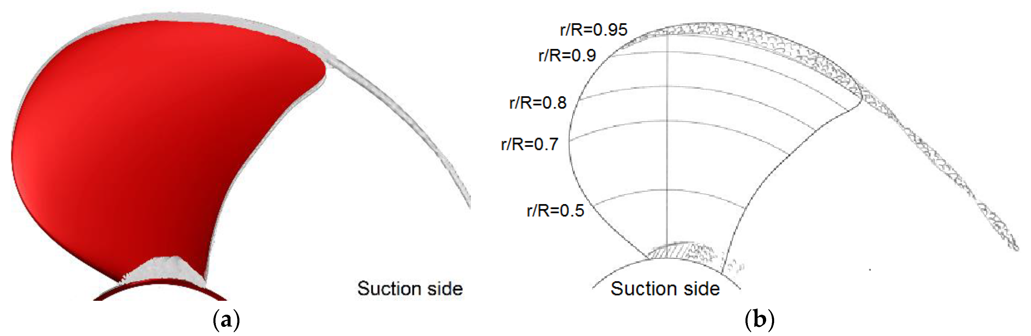
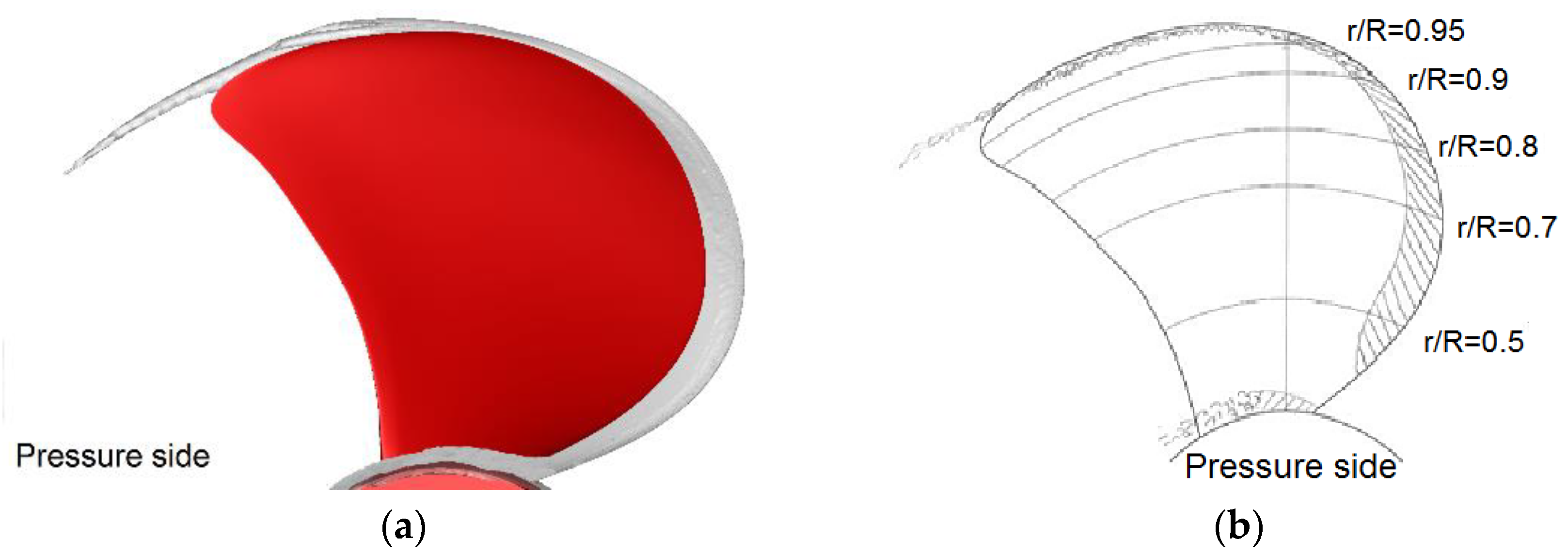
In terms of pressure distribution on the blades, the present computation revealed that the highest values correspond to lower advance ratios, i.e., for heavier loading conditions, as expected. For instance, the non-dimensional pressure computed for
depicted in
Figure 5 unveils rather strong gradients inside the regions around the tips and mid chord of the roots on both sides of the propeller. The same high gradients are located on both leading and trailing edges of the suction side, shown in
Figure 5b, which is not the case on the pressure side where the distribution looks more uniform, except for a limited area which extends between the relative radii of 0.6 and 0.7.
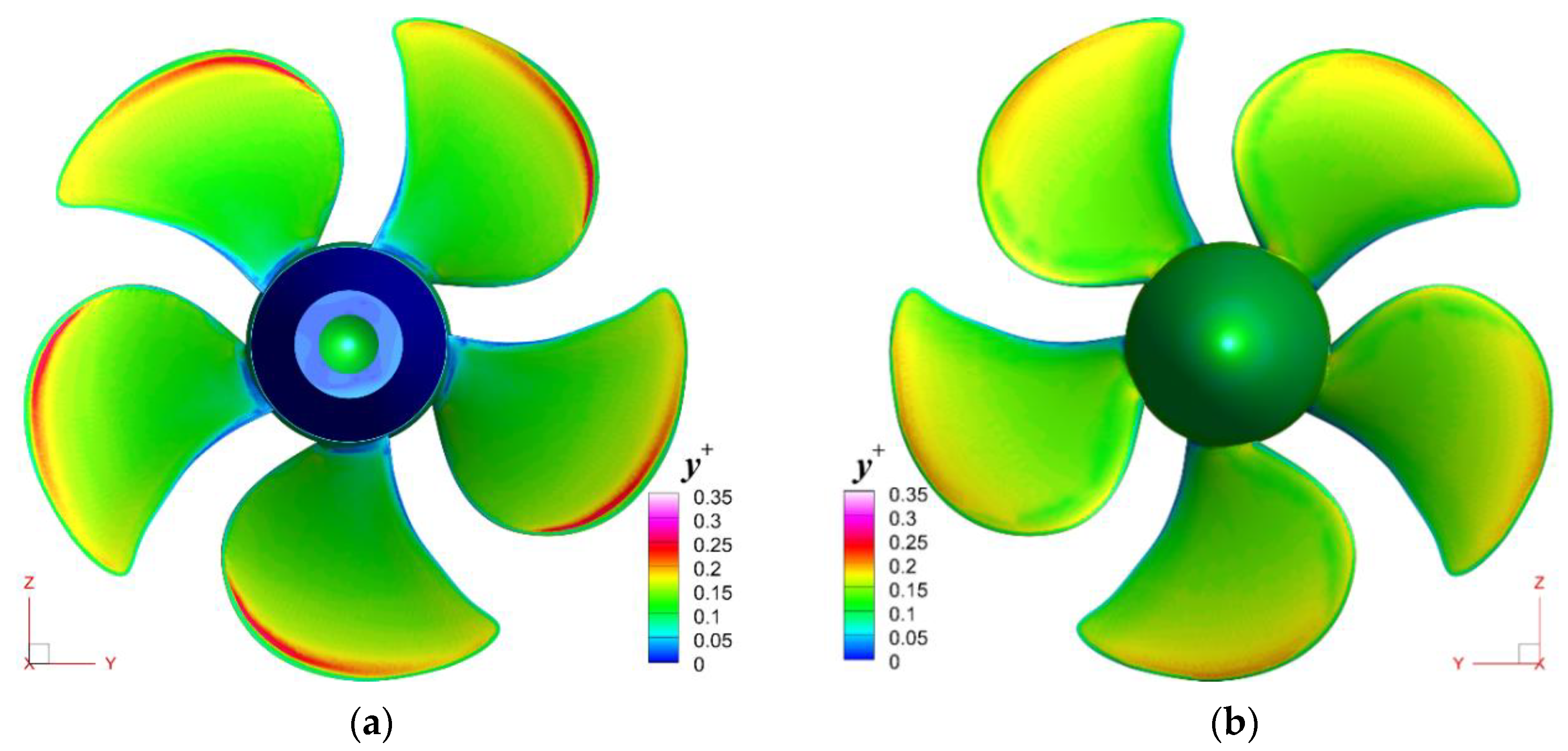
Obviously, the accuracy of the numerical solution strongly depends of the fineness of the spatial discretization. Although not presented here because of limited space reasons, systematic computations have proven that the best matching between the measured and computed pressure coefficients at all the relative radii between the hub and the tip of the propeller were obtained on the finest grids. As mentioned above, the severe restrictions imposed on the cells clustering on the solid surfaces, required by the DES turbulence model, led to a
well below unity, as proven in
Figure 6, which bears out its distribution on each side of the propeller. A maximum value for around the upper part of the leading edge, in the order of 0.3, can be distinguished in the figure. The high resolution of the discretization had to be correlated with small enough time-stepping so that the Courant-Friedrichs-Lewy condition is satisfied. The time-step size for all the simulations reported here is less than 5 × 10
−5 s, so that the Courant numbers could be kept below unity regardless of the value of the oncoming flow velocity. Needless to say, the small time-step value led to high CPU time costs. However, they were finally justified by the good agreement with the available experimental data provided in [
36].
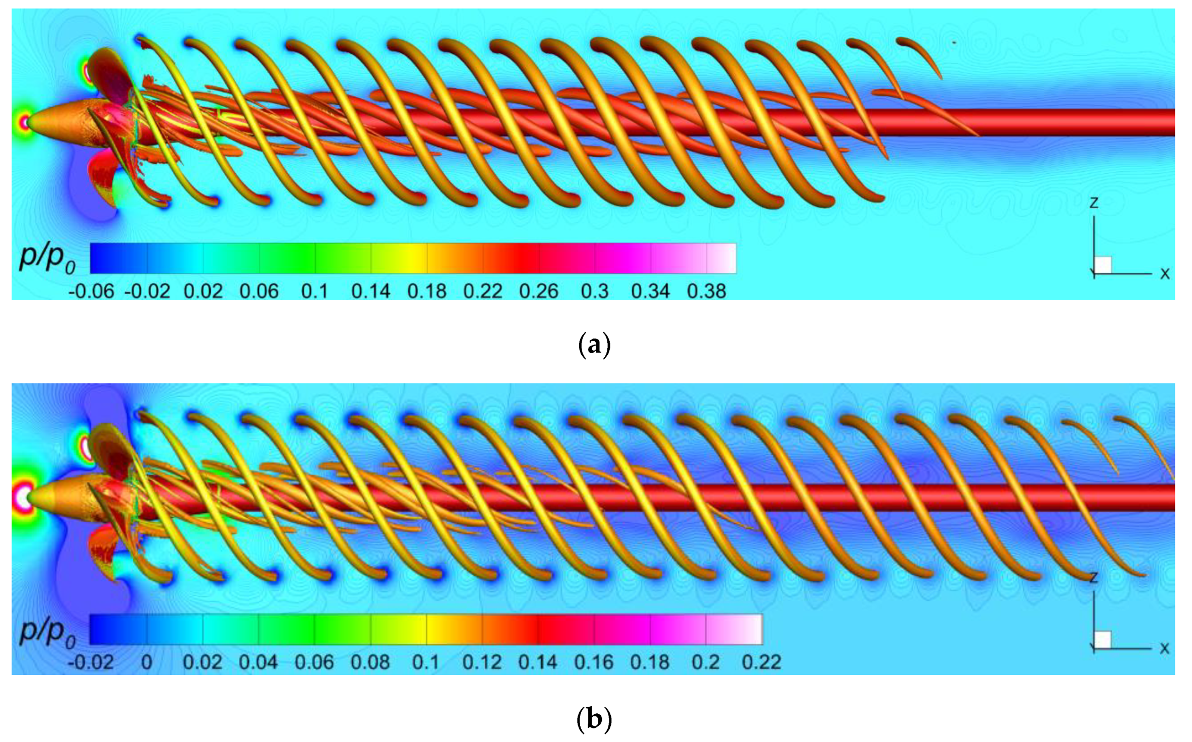
Definitely, the pressure field developed in the wake is always strictly related not only to the pressure distribution on the propeller blades and hub, but also to the vortical structures released by them downstream. This can be clearly seen in
Figure 7, which shows the non-dimensional pressure field computed in the longitudinal plane of symmetry of the computational domain for
and
, respectively.
and
in
Figure 7 are the instantaneous and atmospheric pressure, respectively.
The vortices are represented by the non-dimensional iso-surfaces of the second invariant of the velocity gradient colored by the normalized streamwise velocity, i.e., the component parallel to the free-stream velocity. The locations of the cores, regardless of their intensities, correspond to areas of lower local pressures, as expected. In terms of intensity,
Figure 7 proves that the propagation is dependent on the advance coefficients, i.e., as the advance coefficient increases, the extension of the vortices increases, and the wake remains co-linear with the incoming flow. It is also observed that the pressure intensity in the surrounding areas of the core of the vortex slightly decreases for higher advance coefficients.
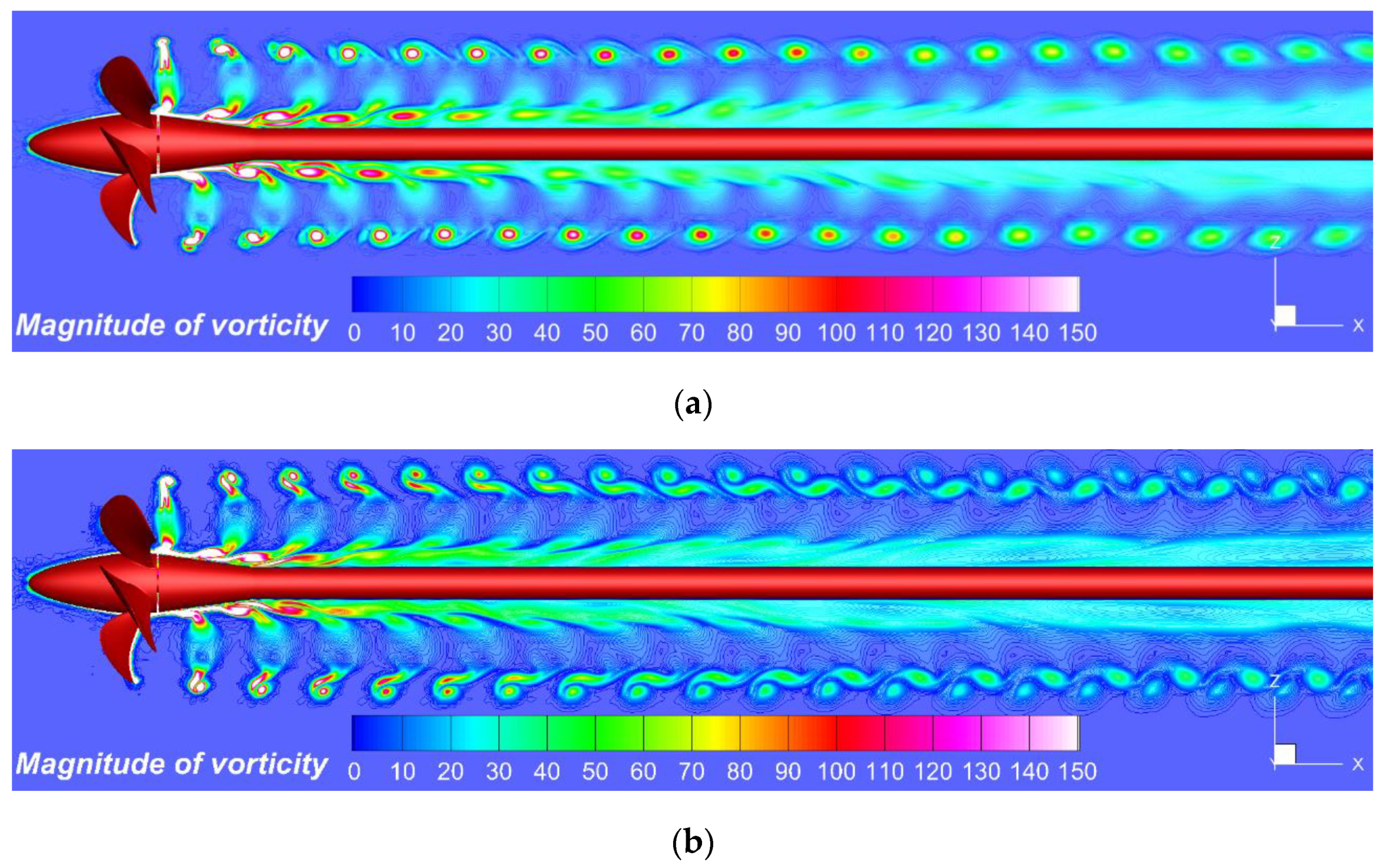
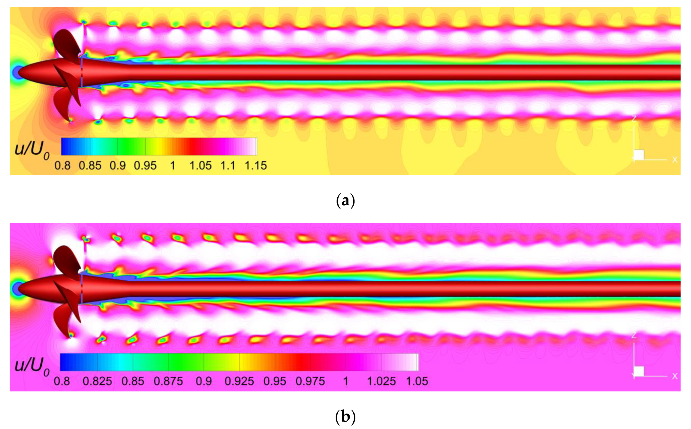
The pressure distribution on the longitudinal plane of symmetry has to be related to the other hydrodynamic parameters that describe the flow mechanism. In order to do that,
Figure 8 proposes a comparison of the vorticity fields, whereas
Figure 9 shows the non-dimensional streamwise velocities drawn for the same two advance coefficients of
and
, respectively.
and
in
Figure 9 represent the instantaneous axial velocity and the incoming flow velocity. The comparison between these figures supports a primary conclusion. To simulate the onset and progression of the vortical structures it is mandatory to use a very fine grid around and in the wake of the propeller. Otherwise, the numerical diffusion will be so large that the onset and progression of these vortices is destroyed by the artificial numerical diffusion. To reduce the need for prohibitive computational resources, an automatic grid refinement based on a regularized version of the Hessian of the pressure is employed in this study.
It has been shown by the author in [
16,
17] that the anisotropic two-equation EARSM non-linear turbulence closure performs better than the linear isotropic
closure with a significant increase of the vorticity and extension of the vortices predicted, with even new structures detected. However, the DES-SST model which is employed in this research proves to behave better since it is able to predict more intense and sustainable vortices, as also mentioned in [
40]. This statement is sustained by
Figure 8 and
Figure 9. The magnitude of vorticity shown in
Figure 8 is expressed in s
−1. Both the axial velocity and vorticity manifest periodic pulses that correspond to the cores of the vortices. Their intensity decreases in the wake because of the viscous dissipation. Strong tip-released structures are shed in the wake, correlating with local maxima of turbulent kinetic energy. The good agreement between the velocity and vorticity is explainable since they derive from the other. Because the hybrid LES model DES-SST only works with no-slip conditions for velocity on the solid boundaries, it proves to be more reliable since it does not employ any wall functions.
The acceleration of the flow right behind the propeller determines a slight reduction of the radial position of the vortex cores. Further downstream, the helices formed by the tip vortices become stable and remain located on a circular cylinder. In the DES-SST approach, the tip vortices are maintained much further in the wake, which is not the case with the RANS models, which yields tip vortices but they vanish more or less rapidly in the wake depending on the level of anisotropy associated with the turbulence model. These remarks were also made in [
40,
41].
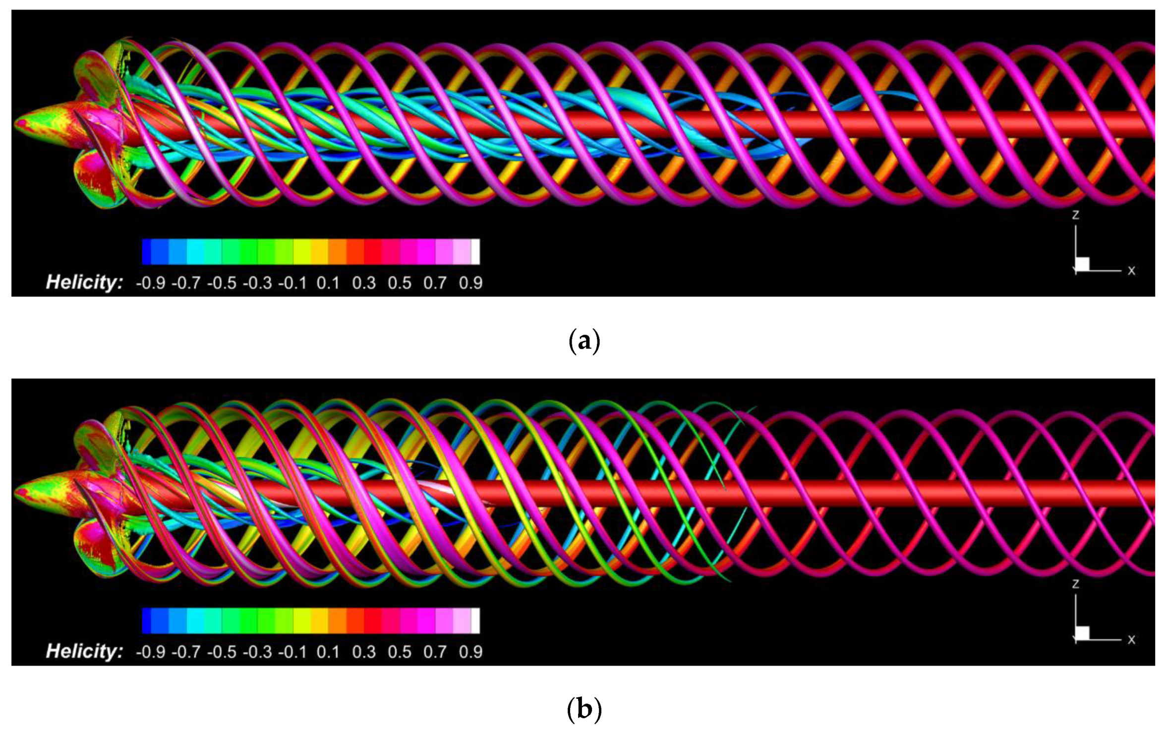
Regardless of the advance ratio, the trajectory of the tip vortex in the longitudinal plane inclines towards the hub on the whole, suggesting a contraction of the trajectories of the tip vortices, which becomes more significant when the advance ratio decreases. The helical pitch of the vortices is constant, a fact that suggests that no numerical dissipation takes place. This is a merit of the solver, which indicates suitable conservation properties, and also of the mesh clustering downstream of the tips, which proves to be non-dissipative. The intensity of the vortices gets weaker further in the propeller wake, a fact which is seemingly due to the viscous interaction with the rest of the fluid. As a result, the vortical structures either vanish, as
Figure 10 bears out, or simply collapse into each other within an area of distortion.
Figure 10a shows the vortices computed at an advance coefficient of
, whereas
Figure 10b shows the solution computed for
. Both solutions are drawn at
sec., therefore when the propeller has already made 250 complete rotations. For higher advance coefficients, with the increase of the downstream distance, the propeller trailing vortex wake restores gradually to the free-stream flow and the fluctuation of the circumferential distribution of axial velocities becomes weaker, as depicted in
Figure 9. A secondary vortex system is released by the trailing edges of the blade roots. The junction between the blade and hub determines the occurrence of a horseshoe-like vortex of a lower intensity than the tip vortex, which is therefore washed away in the downstream. The mechanism of its generation and development was formerly described in detail in [
42,
43], therefore no more discussion will be made herein.
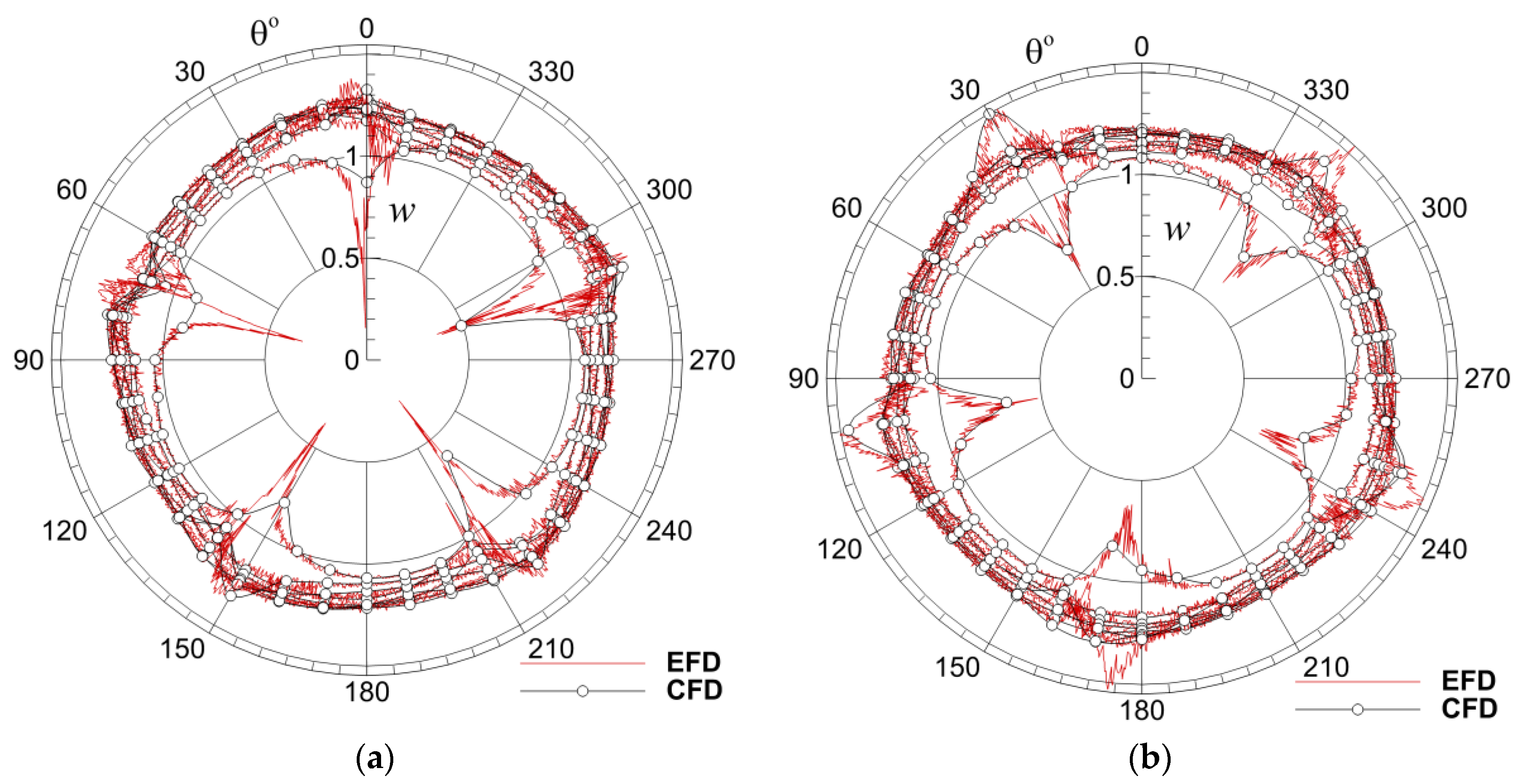
In the following, an analysis of the wake based on several detailed comparisons with the LDV measurements reported in [
44] is proposed as an additional validation of the computational method. Five relative radii ranging from
to
are considered in the polar representation of the wake depicted in
Figure 11 for two different distances measured from the propeller center towards the downstream, namely
, shown in
Figure 11a, and
in
Figure 11b.
The figure shows the angular variation of the axial wake computed as , whereas is the rotation angle of the propeller. Both numerical solutions refer to sec. The experimental data are represented by solid lines, whereas the numerical solutions by symbols. At first glance, one may notice that the agreement with the LDV data is rather good despite the differences induced by the data filtering. This statement is valid for most of the data. Seemingly, this is the merit of the fine discretization around the blades as well as of the efficiency with which the automatic mesh refinement works.
Nevertheless, there are some differences which can be seen in the correspondence of the blade tips. This may suggest the need of extending the comparative analysis to the other wake components. Consequently, the tangential and radial wake distributions will be subjected to study in the following figures.
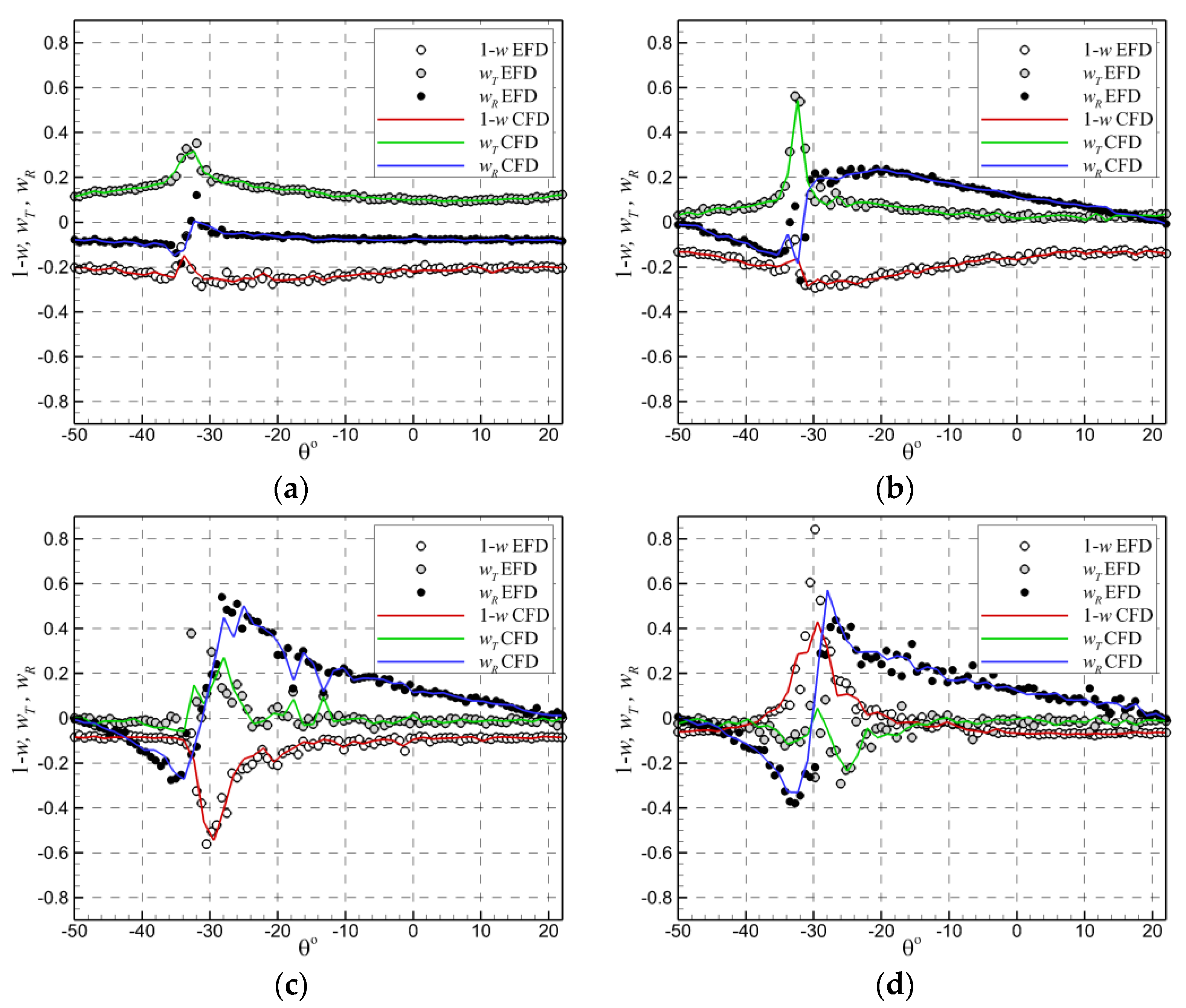
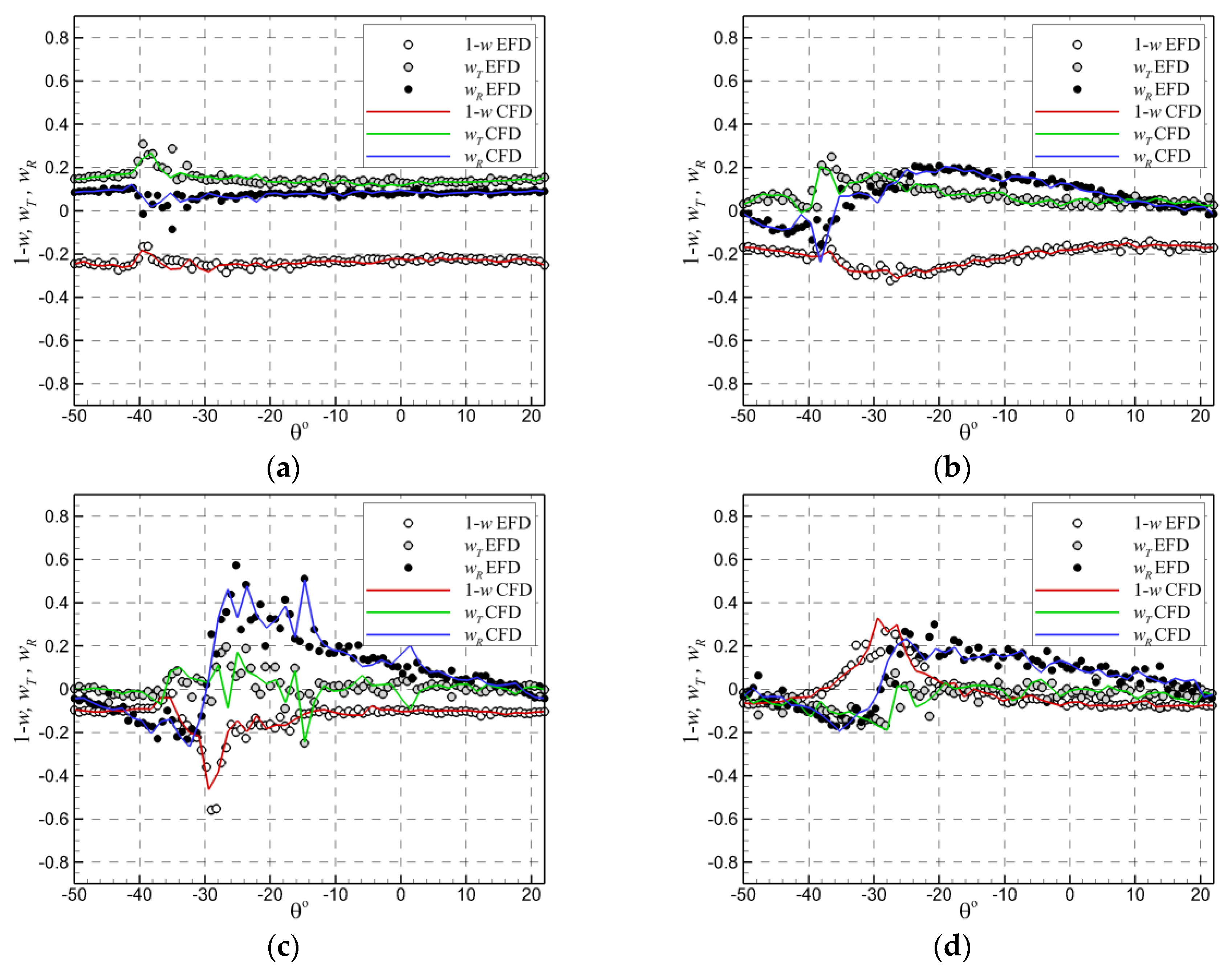
Figure 12 and
Figure 13 show comparisons between the computed and measured tangential and radial wakes computed for a blade at two different axial locations, i.e.,
x/
D = 0.1 and
x/
D = 0.2, respectively. Numerical solutions are drawn with lines, whereas the experimental data provided in [
44] with symbols. For the sake of similarity with the experimental data, the circumferential wake distribution is given within the range of
only, which is a sector that completely covers the first blade. The tangential wake is defined as
, whereas the radial one as
.
and
are the tangential and radial components of velocity. Axial velocities are positive in flow directions and radial velocities are positive for increasing radii, while tangential velocities are positive for the direction of rotation. The solutions are reported for the relative radii of 0.7, 0.9, 0.97 and 1.0 for both axial locations. They all refer to
sec.
The comparisons made for
x/
D = 0.1 shown in
Figure 12 reveal an overall satisfactory agreement between the numerical solution and the experimental data [
44]. However, small differences can be observed around the tip of the blade for the axial wake computed at
r/
R = 1.0. Although the experimental data show some spare points due probably to the filtering, the numerical solution seems to slightly under-predict the wake intensity. This fact may suggest either an insufficiency of the grid resolution in that region or a failure of the solver in capturing properly the separation that takes place there. In either case, more detailed investigations are obviously required to get a better understanding of the reason for that local discrepancy.
A similar conclusion may be drawn from
Figure 13, which depicts the same comparisons of the wake components measured [
44] and computed at
x/
D = 0.2. Comparing
Figure 12 with
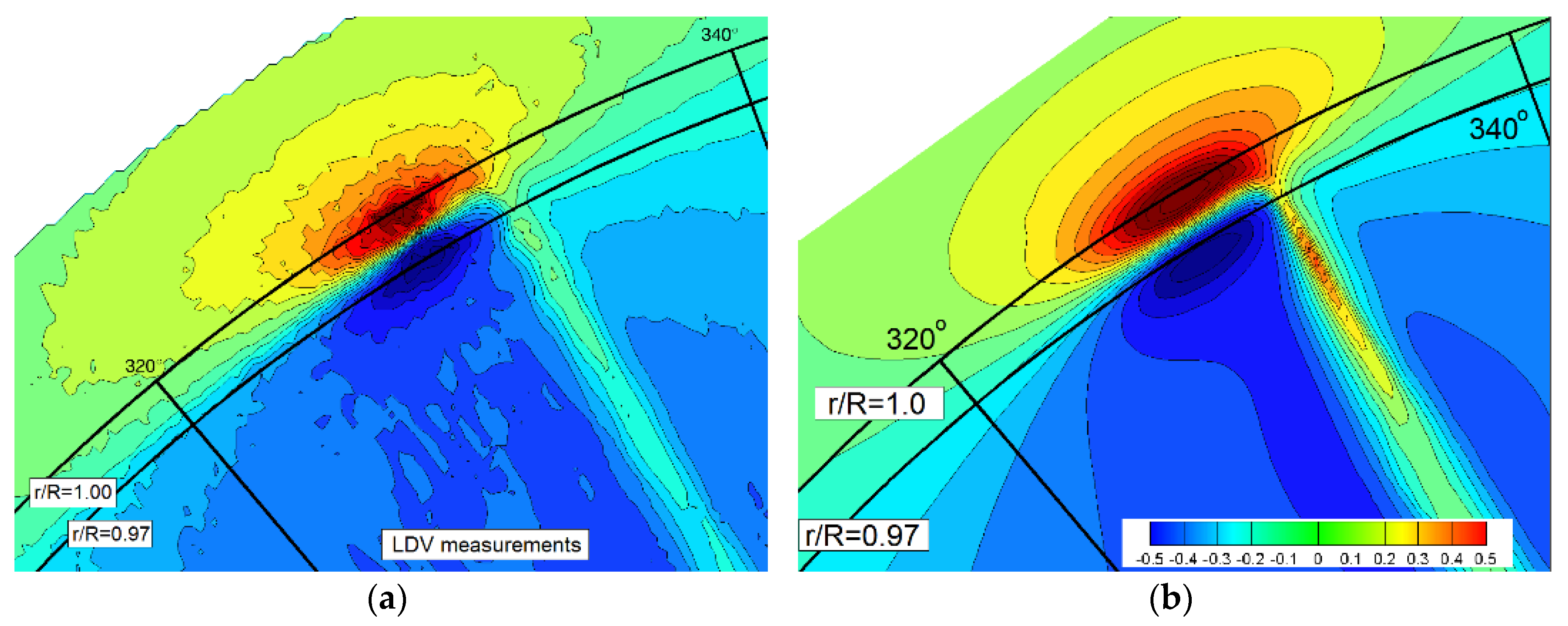
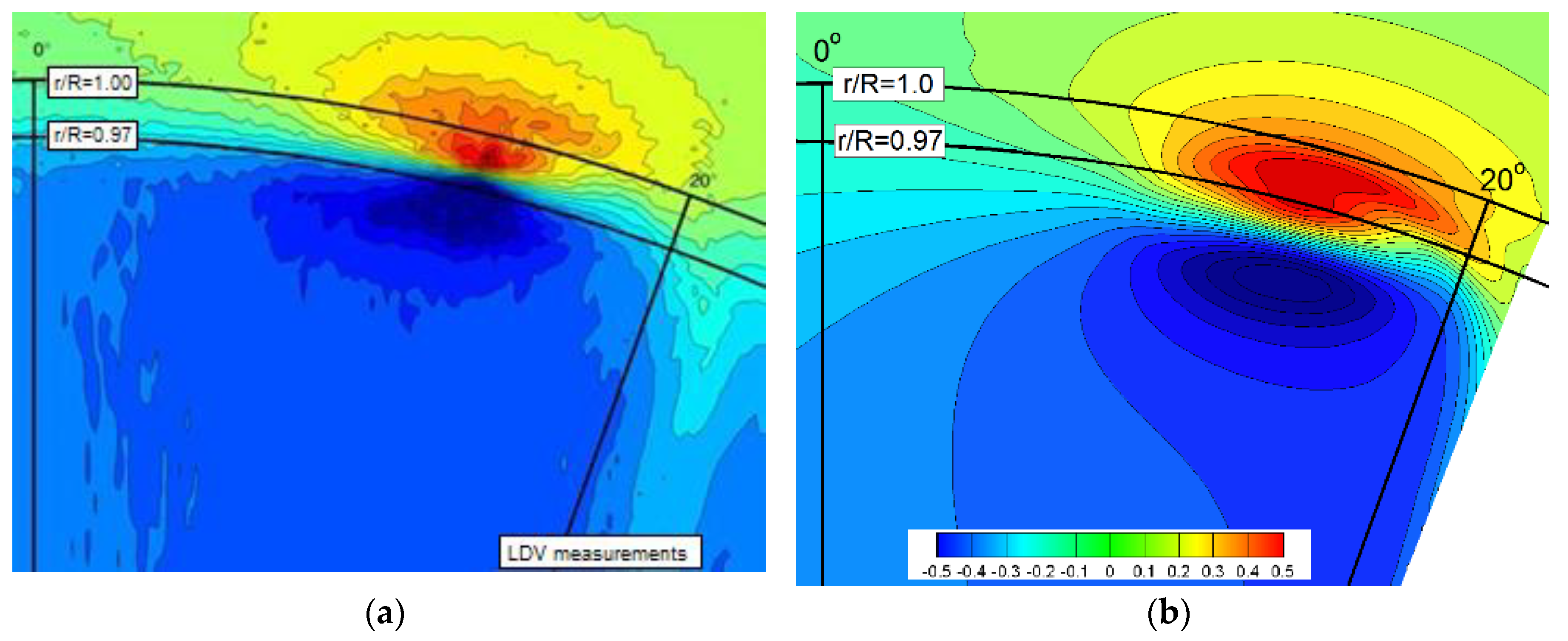
Figure 13, one may notice that because of the viscous dissipation, the wake intensity decreases as the distance from the propeller increases, a fact that confirms the expectations. The conclusions above are sustained by the comparisons of the normalized axial velocities computed and measured [
44] (pictures provided courtesy of Lars Lubke at Schiffbau-Versuchsanstalt (SVA) Potsdam [
45]) at
x/
D = 0.1 and
x/
D = 0.2, shown in
Figure 14 and
Figure 15, respectively. It is worth emphasizing that the agreement is satisfactory although both comparisons reveal that the numerical solution is slightly over-predicting the extension of the axial wake at both locations considered. Nonetheless, the magnitude of the numerical solution is below the measured data within a limited region strictly confined to the blade tip, as also seen in
Figure 12d and
Figure 13d.


