
Path Planning of an Unmanned Surface Vessel Based on the Improved A-Star and Dynamic Window Method

1
School of Automotive Engineering, Changshu Institute of Technology, Suzhou 215506, China
2
Merchant Marine College, Shanghai Maritime University, Shanghai 201306, China
*
Author to whom correspondence should be addressed.
J. Mar. Sci. Eng. 2023, 11(5), 1060; https://doi.org/10.3390/jmse11051060
Submission received: 16 April 2023
/
Revised: 11 May 2023
/
Accepted: 12 May 2023
/
Published: 16 May 2023
(This article belongs to the Special Issue Application of Artificial Intelligence in Maritime Transportation)
Abstract
:In order to ensure the safe navigation of USVs (unmanned surface vessels) and real-time collision avoidance, this study conducts global and local path planning for USVs in a variable dynamic environment, while local path planning is proposed under the consideration of USV motion characteristics and COLREGs (International Convention on Regulations for Collision Avoidance at Sea) requirements. First, the basis of collision avoidance decisions based on the dynamic window method is introduced. Second, the knowledge of local collision avoidance theory is used to study the local path planning of USV, and finally, simulation experiments are carried out in different situations and environments containing unknown obstacles. The local path planning experiments with unknown obstacles can prove that the local path planning algorithm proposed in this study has good results and can ensure that the USV makes collision avoidance decisions based on COLREGs when it meets with a ship.
1. Introduction
In recent years, due to global warming, increasing environmental pollution, and the scarcity of land resources, countries around the world have paid more attention to the development of marine resources [1], which has led to the rapid development of intelligent maritime technologies such as unmanned surface vehicles (USVs) and underwater robots. As an intelligent robot, ASV can perform tasks independently without human intervention [2,3]. It is a surface operating platform with the advantages of a small size and stealthiness. Therefore, it is mainly used to perform hazardous missions [4]. USVs play an important role in civil and military fields such as environmental monitoring, hydrographic exploration, offshore patrol, maritime search and rescue, and long-range reconnaissance [5,6]. During the navigation of USVs, they are affected not only by the known static environment (shore base, shoals, islands, etc.) but also by unknown dynamic vessels and unknown static obstacles (pontoons, offshore operating platforms, etc.) [7]. In order to ensure safe navigation, USVs will first perform global path planning based on known static obstacles in the navigation environment during operation, then perform real-time detection of the dynamic ocean environment [8], and finally implement local dynamic path planning in combination with COLREGs. During the process of the dynamic path planning, when the vessels are in sight of one another, only by considering the rules of collision avoidance can the USV in sailing be guided accurately [9]. At present, there are also many studies focusing on ship collision avoidance algorithms; Zhang et al. [10] proposed a distributed intelligent anti-collision decision support formulation and designed a linear extension algorithm for both course alteration and speed reduction to keep clearance of all the target ships, which proves that anti-collision formulation can avoid collision when all ships have complied with COLREGs as well as when some of them do not take actions. Cai et al. [11] proposed a Collision Risk Index of Ferry (CRIF) based on the behavior of ferries and multiple target ships, which makes it possible to assess real-time collision risk during crossing and to integrate the collision risk of each voyage based on historical encounter scenarios. Xu et al. [12] proposed a modified path-following control system using the vector field method for USV. Unlike other methods, they considered the coupled path following and collision avoidance task as a whole. Finally, their proposed method allows the USV to follow a predetermined path while automatically avoiding obstacles. Zhang et al. [13] proposed a modified path planning method called RRTes, which simultaneously considers the ship draft and UKC to avoid grounding as well as ship maneuverability constraints and COLREGs to identify ship dynamic collision risk. Therefore, in addition to global path planning, USVs need to have the ability to plan paths in a dynamic environment. In the current research on USVs [14], autonomous collision avoidance technology is a key technology that has not been surpassed in the development of unmanned vessels and is a prerequisite for USVs to navigate safely in dynamic environments.
Based on COLREGs, Almoaili et al. [15] propose a near-optimal algorithm to find a feasible path for UGVs (Unmanned Ground Vehicle) in a static environment, and the performance of the proposed algorithm was compared with other well-established algorithms in the path planning literature such as A* using a simulator developed for this purpose. Wang et al. [16] designed three-dimensional path planning and security event-triggered cooperative path tracking for a multi-disc autonomous underwater glider (AUG) considering the presence of underwater obstacles and denial-of-service (DoS) attacks. In the study by Jabbarpour et al. [17], a new ant-based path planning approach that considers UGV energy consumption in the IPTS planning strategy is proposed. This method is called Green Ant (G-Ant) and integrates an ant-based algorithm with a power/energy consumption prediction model to reach its main goal, which is providing a collision-free shortest path with low power consumption. Han et al. [18] propose a path planning method based on the multi-strategy evolutionary learning artificial bee colony algorithm. Thoresen et al. [19] propose a new method of path planning for UGVs on terrain, and the proposed path planning method is based on the Hybrid A* algorithm and uses estimated terrain traversability to find the path that optimizes both traversability and distance for the UGV. Shin et al. [20] proposes a model predictive path planning algorithm by employing a passivity-based model predictive control (MPC) optimization setup. Chen et al. [21] introduce a new meta-heuristic path planning algorithm, the Cuckoo-Beetle Swarm Search (CBSS) algorithm, to solve the path planning problem for heterogeneous mobile robots. Through domestic and international research, it has been found that there are few studies in global path planning that can ensure path safety while also considering path economy. In local path planning, unknown static obstacles are rarely considered to be introduced into the environment. Therefore, the improved A * algorithm is used in global path planning to generate routes that are both safe and cost-effective. Unknown static obstacle evaluation factors are introduced into the evaluation function of the dynamic window method (DWA) in local path planning. This improves the sensitivity of the algorithm in local path planning. This article integrates global and local path planning, which can provide certain feasible suggestions for route planning before unmanned vessel navigation and collision avoidance during navigation.
2. Global Path Planning of USV Based on an Electronic Navigation Chart
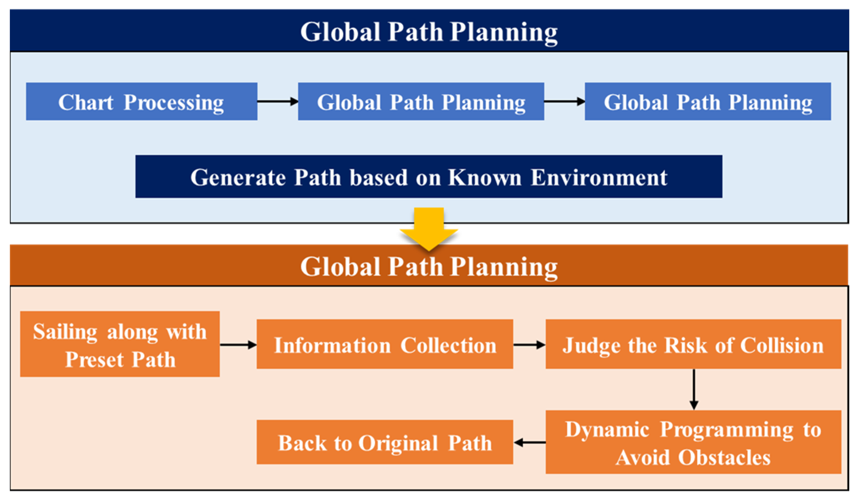
In order to realize the autonomous navigation of the USV under mutual visibility conditions, the navigation environment is established based on a 5 m depth contour according to web charts. It is based on the surface data in the ECDIS data, and rendering is performed using tools such as Mapbox to achieve the display of basic surfaces such as land, shoals, and bathymetric surfaces. Java’s SpringBoot framework is used as the main body of the program, the ORM (Object Relational Mapping) framework of the MySQL database is Mybatis, the Druid is used as the Connection pool of the MySQL database, and the JedisPool is used as the Connection pool of the Redis database. A front and rear nonseparation strategy is adopted. The security optimization objectives for global path planning are determined, and a global path planning model is established. The flowchart of our work is shown in Figure 1. This work includes global path planning and local path planning. The global path planning is the generation of a path based on known static obstacles, including chart processing, path planning, path smoothing, etc. Local path planning is the dynamic adjustment made by ships when navigating along the globally planned path. During navigation, there may be static and dynamic obstacles that are not displayed on the chart, and safe collision avoidance actions need to be taken to avoid collisions. After avoiding collisions, it is necessary to return to the global planning path.
2.1. Chart Data Processing
First of all, the surface data rendered in different colors in the nautical chart are processed by pixel threshold segmentation. Among them, the processing that satisfies the water depth constraints is the navigable area, and the others are the obstacle area. Using electronic charts displayed on the web as the initial experimental environment, a global path planning experimental model is constructed for a portion of the chart areas with a latitude range of 30°9.627′ N–30°21.306′ N and a longitude range of 121°52.356′ E–122°8.543′ E. The values of different chart information (R, G, B) are shown in Table 1.
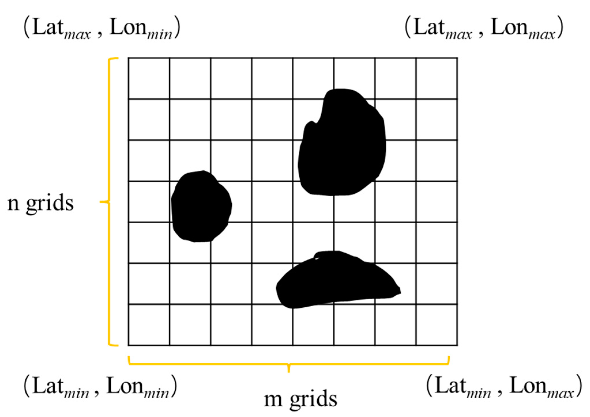
Second, the point and line data that hinder navigation in the screening experiment area are drawn in the experiment environment model. Next, after constructing the nautical chart data into a rasterized environment model, the generated path is the grid position point in the Cartesian coordinate system. In order to be able to guide the navigation of the USV in practice, it is necessary to convert the grid nodes and the geographic coordinate system (longitude, latitude). The coordinate conversion calculation principle is shown in Figure 2. Figure 2 shows a chart area where the maximum and minimum latitudes are and and the maximum and minimum longitudes are and . The corresponding number of horizontal grids is , and the number of vertical grids is . The conversion formula between latitude and longitude and grid coordinates is as follows:
Among them, and represent the position point coordinates of the unmanned ship during navigation, and and represent the horizontal and vertical coordinates in the grid map, respectively.
2.2. Improved A-Star Algorithm
As a commonly used heuristic path search algorithm, the A-star algorithm is widely used in the field of global path planning [22]. Its search methods include four-connected area search and eight-connected area search. Considering the movement characteristics of the USV in the ocean [23], this paper uses the search method of eight-connected areas to search navigable waters. The heuristic function of the improved A-star algorithm is defined as follows:
where is the actual distance cost from the starting point to the current node, is the estimated distance cost from the current node to the target node [24], and is the hazard function that uses the Voronoi field to add hazards to the grid. The A-star algorithm only uses the path length as a heuristic function, and the planned path often approaches obstacles, which cannot effectively guide USV to navigate safely and smoothly. This article improves the evaluation function of the A-star algorithm by using the concept of establishing navigation boundaries based on the Voronoi field algorithm, the definition of which is as follows:
where is the distance from the current node to the obstacle, is the distance from the current node to the Voronoi boundary, is a constant that controls the decay rate of the potential field, and is a constant controlling the maximum operating range of the potential field.
In the process of unmanned ship navigation, not only should the constraint of water depth be considered, but a certain safe distance should also be maintained between the generated path and obstacles. The evaluation functions of each grid after adding hazard levels can be defined as:
is the Voronoi field value at the current node, and D is the safety constraint distance.
3. Local Path Planning of USV
3.1. Collision Avoidance Decision Based on the Dynamic Window Method
First, we establish the motion model of the USV (linear velocity, angular velocity, etc.). Second, a set of navigable speeds including linear and angular velocities is established under the constraints of the motion model and the distribution of obstacles in the motion environment [25]. Finally, the speed vectors under the navigable speed set are sampled, and the predicted trajectory of each speed vector in the next time period is solved according to the sampled speed vectors [26]. Finally, the evaluation function is used to optimize the trajectory, and the speed combination corresponding to the optimal trajectory is used as the navigation speed in the next period of time [27].
The movement state of the USV during navigation is shown in Figure 3. Assume that the current given linear velocity and angular velocity vector is , the current two-dimensional position coordinate is , and the included angle with the abscissa is [28]. The motion model of the USV is shown in Formula (5):
After the USV model is established, the trajectory of the USV in the next sampling period can be predicted according to the motion model. The speed space available for sampling in actual voyages is limited, which is determined by the following three aspects:
- (1)
- Velocity constraints
Suppose the maximum linear velocity of the USV is , the minimum linear velocity is , the maximum angular velocity is , and the minimum angular velocity is [29]. Then, the set of velocities between the maximum value and the minimum value is:
- (2)
- Performance constraints of USV
Assuming that the linear velocity and angular velocity vector of a given USV at a certain moment are , and its maximum linear acceleration and maximum angular acceleration are and [30], then the speed set constrained by the power device is:
- (3)
- Stopping distance constraint
Assuming that is the shortest distance between the end of the USV-predicted trajectory and the obstacle, and are the maximum stopping linear acceleration and maximum stopping angular acceleration, respectively [31]; then, the speed set constrained by the stopping distance is:
In summary, if the USV is to sail safely to the destination, the speed space needs to meet the above three constraints. Assuming that all navigable speed sets of USV in the space are , then is the intersection of the speed sets under the above three constraints.
3.2. Acquisition of Optimal Trajectory
The acquisition of the optimal trajectory is divided into two parts: trajectory preprocessing and trajectory evaluation, and the operation is as follows:
- (1)
- Trajectory preprocessing
Dynamic ship risk detection is the process of screening and predicting trajectories, as well as the operation of determining the timing of collision avoidance. Its principle is shown in Figure 4. The distance between the sampling point of the predicted trajectory and the corresponding position point of the obstructed ship during the period is calculated, and the CPA is adopted. When the distance encountered recently is less than the set safety distance, it indicates a risk of collision. The length of the USV is set to 3 to 11 m, and the draft is less than 2 m. The size of the target ship is set to twice that of the USV, and the draft is 3 m.
When ships perform collision avoidance operations in head-on situations and crossing situations, according to the requirements of the COLREGs, the give-way ship should turn to starboard to avoid stand-on ships. Therefore, the range of angular velocity corresponding to the predicted trajectory will be limited to . This operation needs to be maintained during the avoidance process until no obstructive ship is detected in the predicted trajectory; then, the process ends.
- (2)
- Trajectory evaluation function
On the basis of the constraints of the COLREGs, this paper sets three aspects of speed function, heading function, and distance function to construct the trajectory evaluation function to evaluate the navigable predicted trajectory. The optimal trajectory evaluation function is shown in Formula (9):
where is the trajectory evaluation function, and its maximum value is used to find the optimal solution of the predicted trajectory; the other functions are sub-functions of the predicted trajectory function, and , , , are the weight coefficients of each sub-function. The fastness function is used to evaluate the linear velocity size of the current trajectory, the reachability function is used to evaluate the deviation degree of the predicted trajectory end of the USV from the target point, and the safety functions of known and unknown obstacles and are used to evaluate the safety of predicted trajectories.
The trajectory evaluation function needs to be normalized before evaluation, as shown in Formula (10):
4. Results and Discussion
4.1. Experimental Results of Global Path Planning
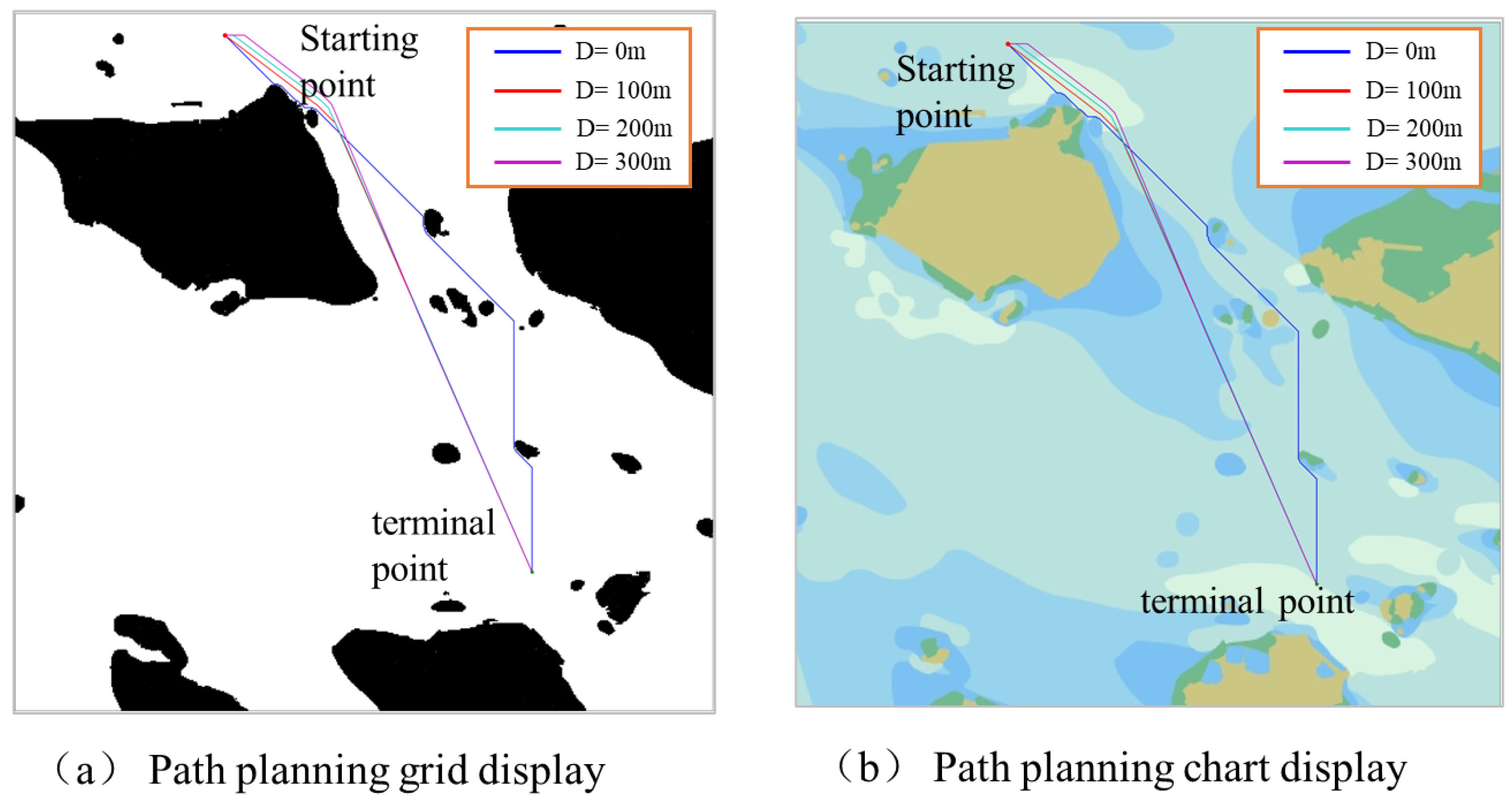
In this paper, the selected nautical chart area is rasterized and divided into 500 × 500 grids, and each grid represents 25 m. Aiming at the maneuverability of the USV, safety distance constraints of 100 m, 200 m, and 300 m are set. The results of global path planning based on different safety distance constraints and smooth optimization are shown in Figure 5, Figure 5a shows the display of the planned path in the grid environment, and Figure 5b shows the planning in the redrawn sea chart water depth environment display of the path.
Figure 5 is a comparison of the experimental results of the traditional A-star algorithm and the improved A-star algorithm under different safety distance constraints. The solid blue line is the result of the global path planning of the A-star algorithm without adding a safety distance constraint. It can be seen that the planned path is close to the obstacle, which will undoubtedly increase the collision between the USV and the obstacle risk. Red, cyan, and magenta are the path planning results of maintaining 100 m, 200 m, and 300 m safety distance constraints, respectively. It can be seen that with the increase in distance constraints, the planned path can maintain distance constraints when approaching obstacles, and the path with a larger safety radius is farther away from obstacles. It can be seen from Figure 5b that the planned paths are all outside the water depth of 5 m, and the proposed method can guarantee the constraint of safe water depth.
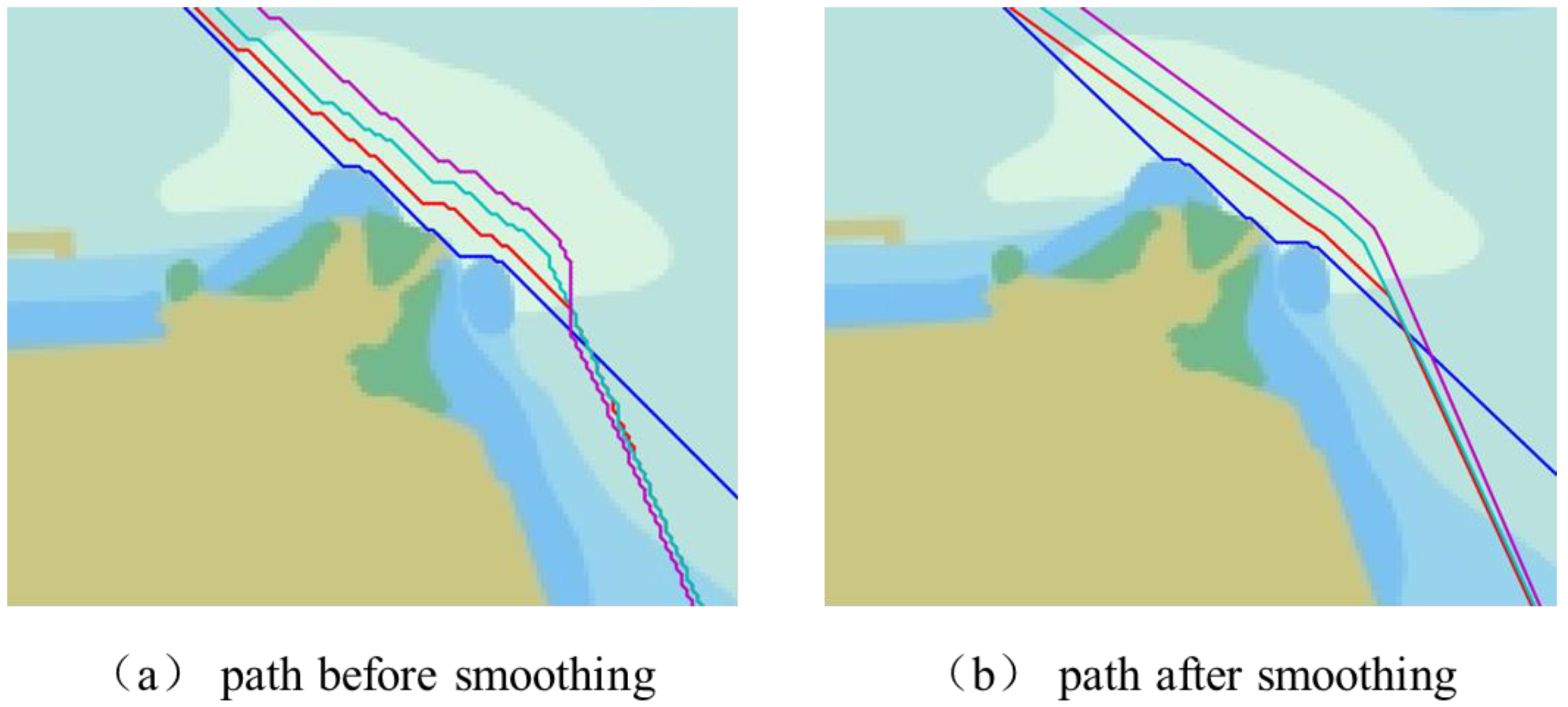
Figure 6 shows the comparison of some planned paths before and after smooth optimization. Figure 6a shows the path before smooth optimization. The number of turns in the path is too many and not smooth, which does not meet the requirements of navigation practice and USV performance; Figure 6b shows the path after smooth optimization. The number of path turns is small, and the smoothness is high, which is of high guiding significance.
Figure 7 shows the distance between the path node and the obstacle under three different safety distances. From the black horizontal dotted line set in the figure, it can be seen that the path node keeps the set safety distance from the obstacle, which can improve the safety factor of the USV during navigation.
Table 2 shows the comparison of path planning results under different safety distances, and it can be seen that the optimized path has good results in terms of length and number of nodes. In terms of path length, the smoothed path has a slight decrease. On the path nodes, there is a significant decrease in the number of smoothed path nodes. The experimental results demonstrate that the path smoothing algorithm proposed in this paper has good performance.
In summary, the global path planning method proposed in this article can achieve dual constraints of water depth and obstacle safety distance, which is in line with the actual requirements of USV navigation.
4.2. Experimental Simulation under Different Encounter Situations
In order to verify the effectiveness of the proposed algorithm in the collision avoidance process, the collision avoidance simulation experiment of USV is carried out in the range of 500 m × 500 m under the three scenarios of head-on, crossing, and overtaking between ships. The simulation parameter setting and algorithm setting of USV are shown in Table 3 and Table 4.
- (1)
- Head-on situation
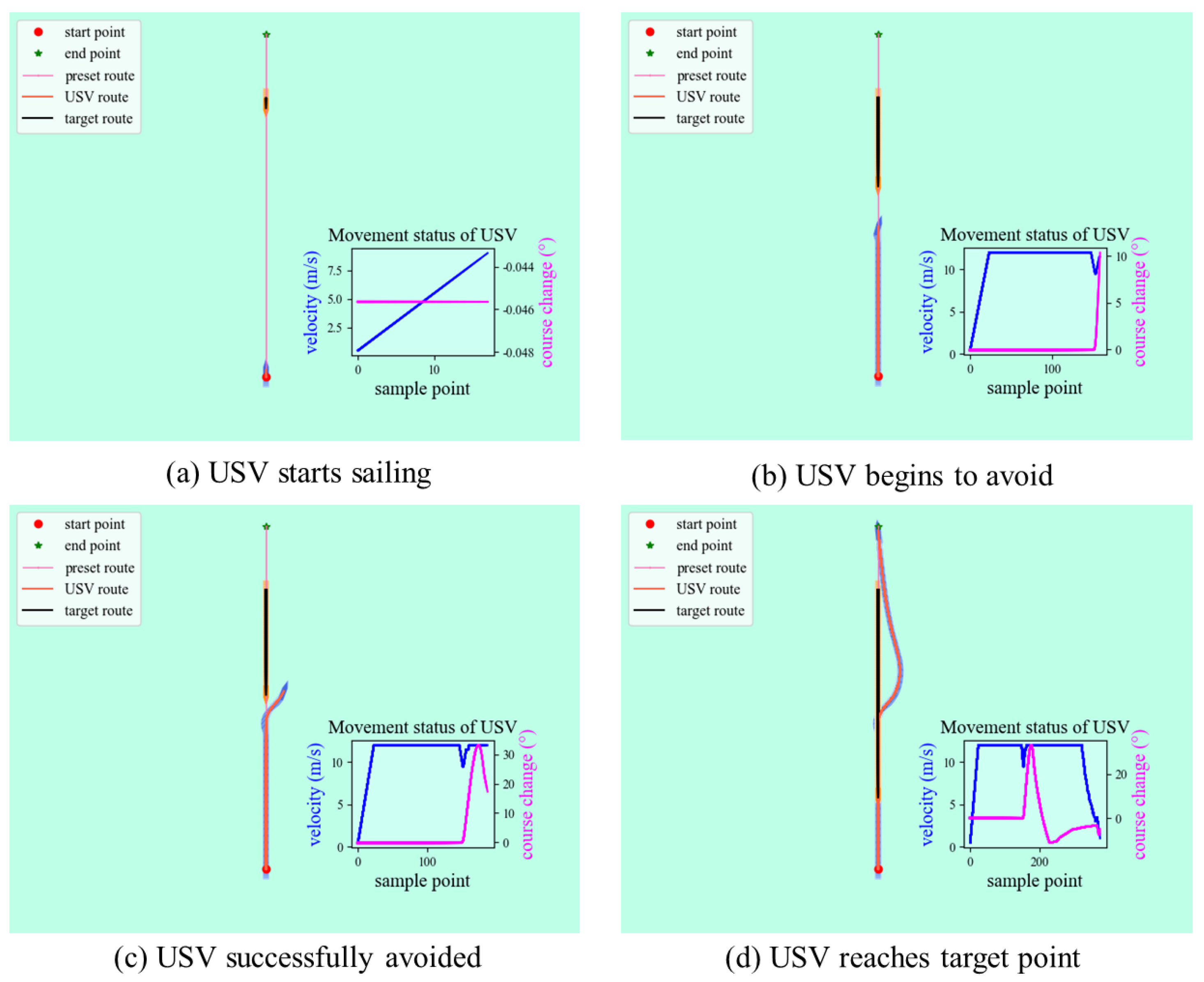
The collision avoidance simulation process in the head-on situation is shown in Figure 7, where the red circle is the starting point of the USV, the green star is the target point of the USV, the pink line is the preset route, the red line is the trajectory of the USV, and black is the trajectory of the target ship in the situation of encountering the USV.
Figure 8a shows the positional relationship between the USV and the target ship before sailing, which can be judged as a head-on situation according to the COLREGs. Figure 8b starts to make a decision for the USV to detect that there is a risk of collision with the target ship. Figure 8c shows that the USV follows the COLREGs and turns starboard to avoid the target ship. Figure 8d shows returning to the preset route after avoiding the target ship and reaching the target point safely.
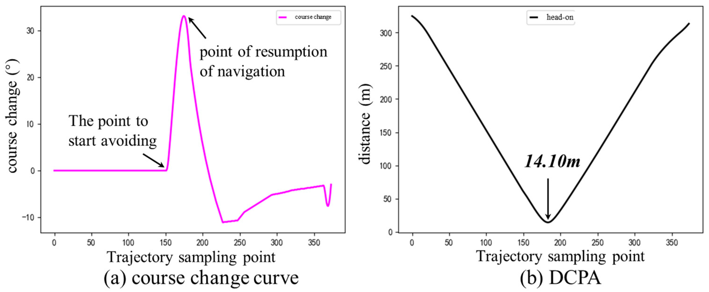
Figure 9 is the heading change curve and the DCPA diagram corresponding to the trajectory sampling points during the entire avoidance process in the USV head-on situation. It can be seen from Figure 9a that near the 150th sampling point, the USV begins to turn and avoid. At this time, the distance between the two ships corresponding to Figure 9b is 50 m, which is in line with the set safety distance. In the process of the encounter, the distance between the USV and the target ship decreases rapidly due to the relatively fast speed of the USV and the target ship. The distance decreases continuously throughout the process, and the nearest encounter distance is 14.10 m. As the process ends, the distance gradually increases.
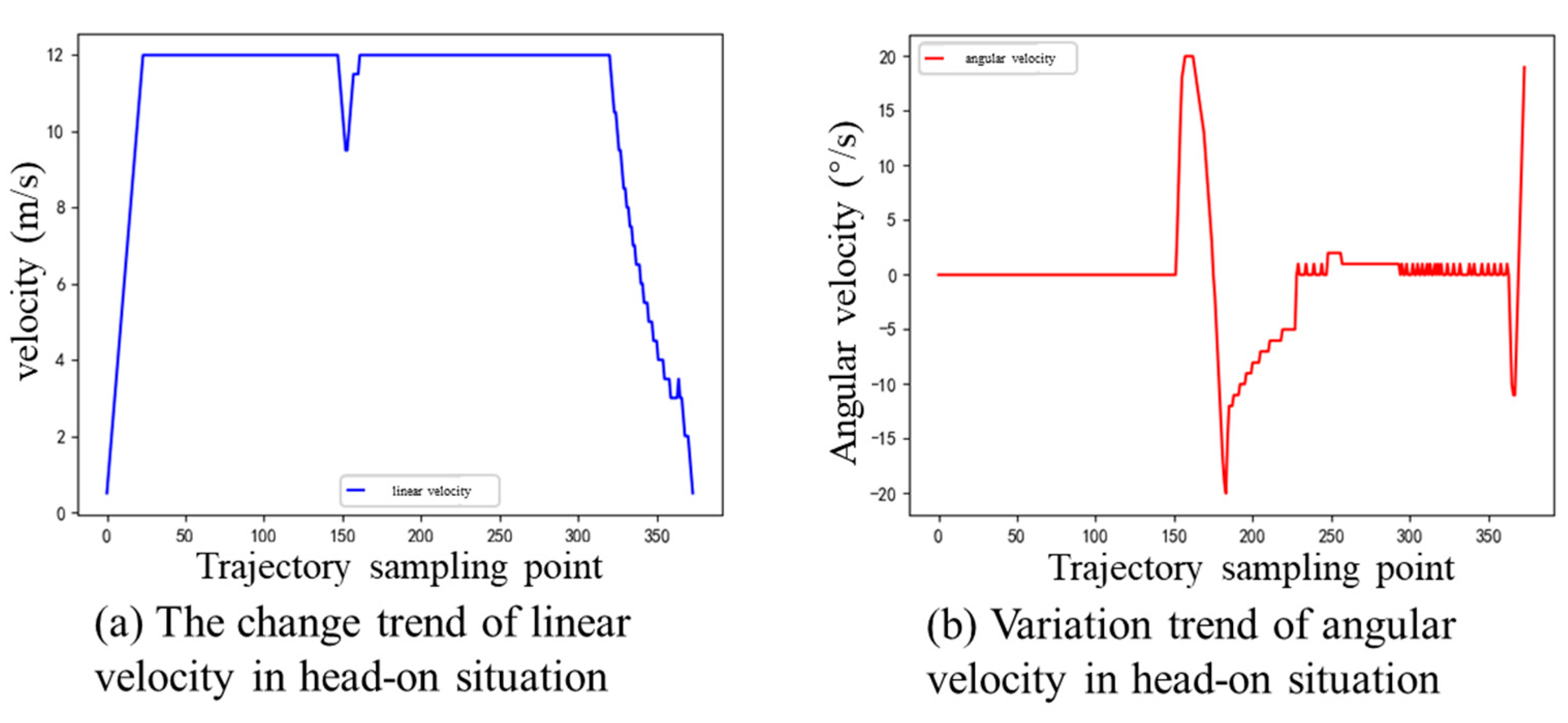
Figure 10 shows the changing trend of linear velocity and angular velocity in the head-on situation. It can be seen from the linear velocity change diagram in Figure 10a that before the collision avoidance process, the USV first accelerates and then has a constant speed; during collision avoidance, deceleration measures are taken; after collision avoidance, the USV accelerates again until it approaches the target point and begins to decelerate. Figure 10b is the diagram of angular velocity change. Before the collision avoidance process, the USV angular velocity is 0, and the navigation is maintained at the predetermined course; during collision avoidance, the USV turns to starboard. From the analysis, it can be seen that the collision avoidance behavior in the encounter process conforms to the COLREGs and the common maneuvering behavior at sea.
- (2)
- Crossing situation
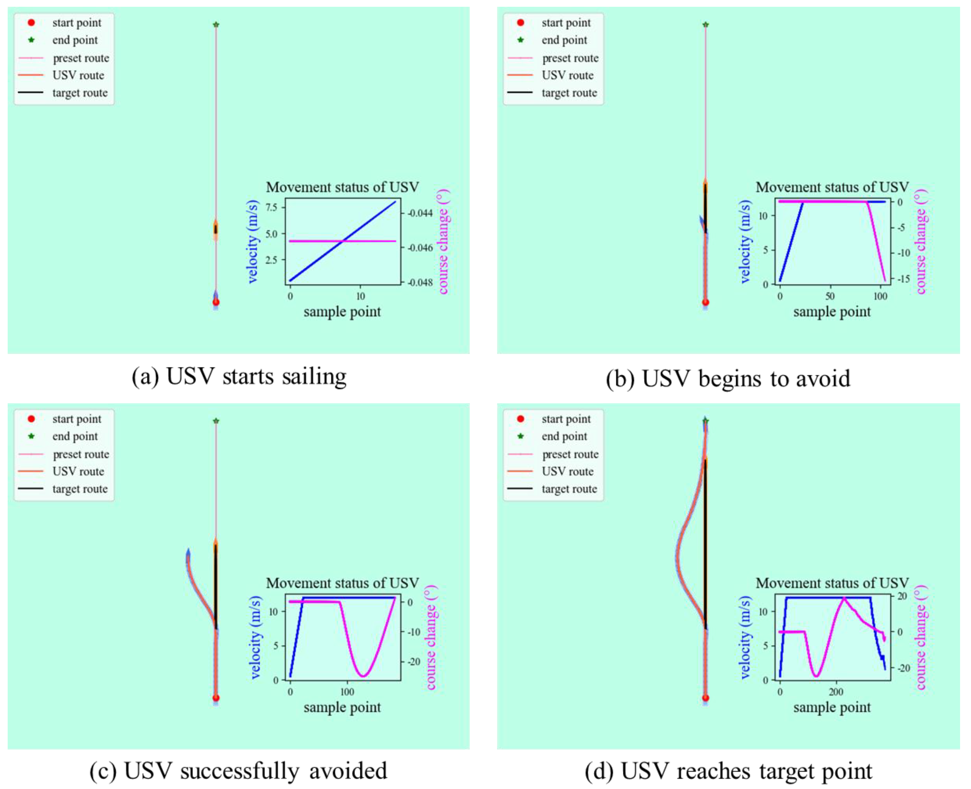
The simulation process of collision avoidance under the crossing situation is shown in Figure 11. Figure 11a shows the positional relationship between the USV and the target ship before sailing, which can be judged as a crossing situation by the COLREGs. Figure 11b starts to make a collision avoidance decision for the USV to detect that there is a risk of collision with the target ship. Figure 11c shows that the USV follows the constraints of the COLREGs and turns to the starboard to successfully avoid the target ship. Figure 11d shows that USV successfully returned to the preset route after safe avoidance and sailed safely to the destination.
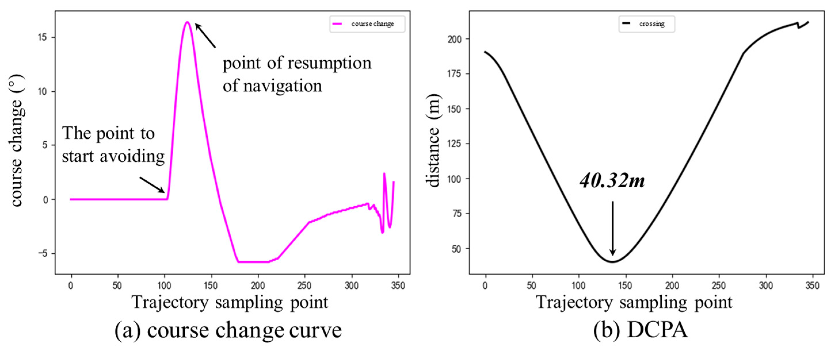
Figure 12 shows the heading change diagram and the DCPA diagram corresponding to the trajectory sampling points during the entire avoidance process in the crossing situation. The first section of Figure 12a shows that the USV keeps a fixed heading when no target ship is detected; the second section is to start to turn starboard to avoid collision when the target ship is detected. The collision avoidance behavior complies with the requirements of the COLREGs. According to the COLREGs, the maximum collision avoidance range is set to 17° since the USV is the give-way ship in the crossing situation, and it should take substantial action to keep well clear and avoid crossing ahead the head-on ship under the allowed circumstances case. The range of collision avoidance ensures the safety of the collision avoidance process, which is consistent with the actual situation of navigation. The third section is the resumption process after collision until reaching the target point. Figure 12b shows the distance of the nearest encounter. It can be seen that the distance between the two ships decreases first and then increases. The distance of the nearest encounter is 40.32 m, which can safely avoid collision.
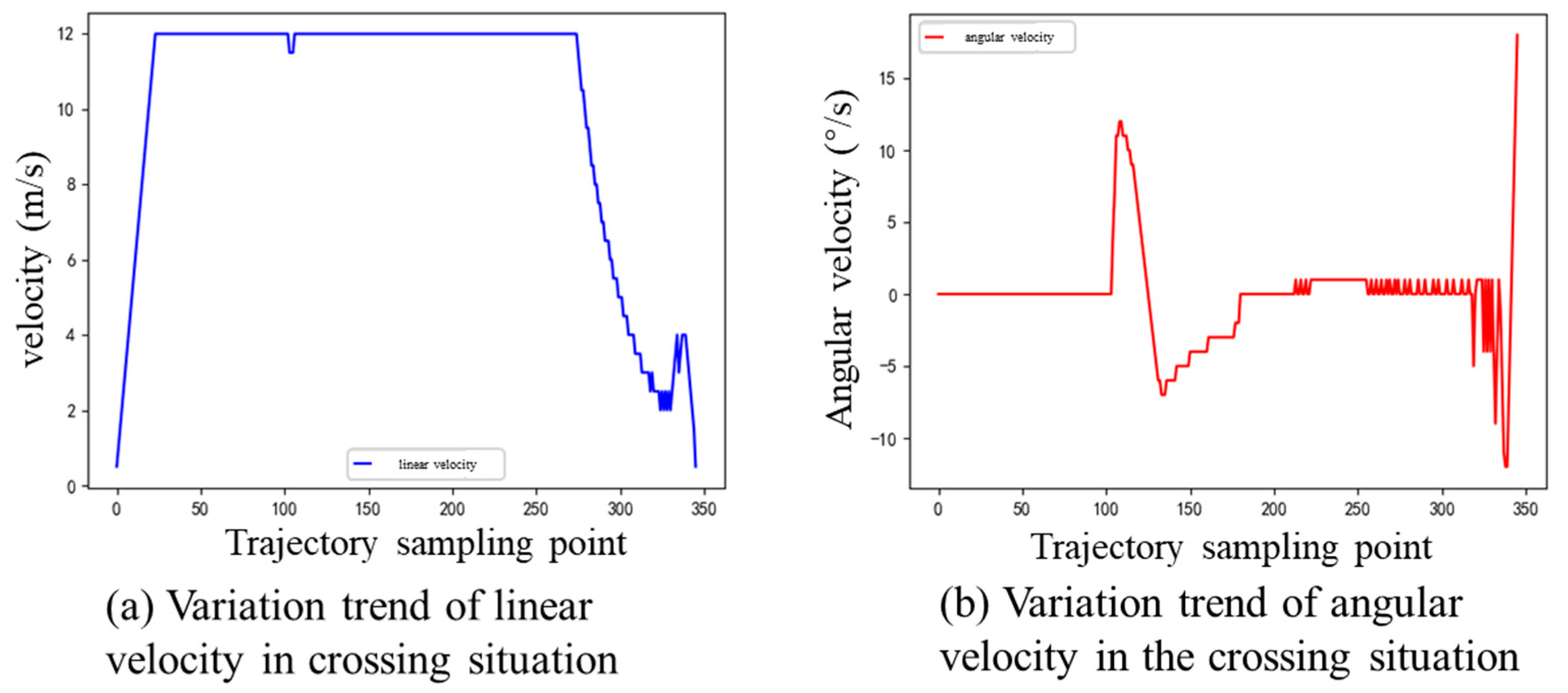
Figure 13 shows the change trend of the line velocity and angular velocity under the crossing situation. Figure 13a shows the trend of linear speed change. During the whole process, speed up first, then sail at the maximum speed and uniform speed and decelerate near the target point. Figure 13b shows the change trend of angular velocity. It can be seen that the course is maintained before collision avoidance. During collision avoidance, turn to starboard to avoid the target ship. Due to the short process, the maximum angular velocity is about 8°/s. After collision avoidance, USV quickly resumes the course.
- (3)
- Overtaking situation
The simulation process of collision avoidance in overtaking situations is shown in Figure 14. Figure 14a shows the overtaking situation. Figure 14b starts to make a decision for the USV to detect that there is a risk of collision with the target ship. Figure 14c shows that the USV follows the constraints of the COLREGs and turns to the port as much as possible to avoid the target ship. Figure 14d shows that the USV returns to the preset route after evading successfully and sails safely to the target point.
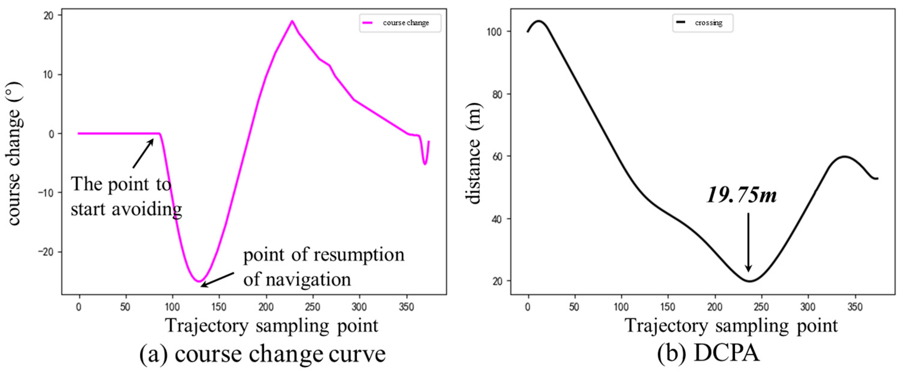
Figure 15 shows the course change curve and the DCPA diagram corresponding to the trajectory sampling point during the whole collision avoidance process under the overtaking situation. The first section of Figure 15a shows that the USV keeps a fixed heading when no target ship is detected. The second section is to start turning to the port to avoid collision when the target ship is detected. The collision avoidance behavior meets the requirements of the COLREGs, and the maximum collision avoidance range is about 27°, which is in line with the actual situation of navigation. The third section is the resumption process after collision until reaching the target point. In Figure 15b, when the encounter distance is less than 50 m, the collision distance will continue to decrease due to the close proximity of the two during the overtaking process, and the nearest encounter distance is 19.75 m.
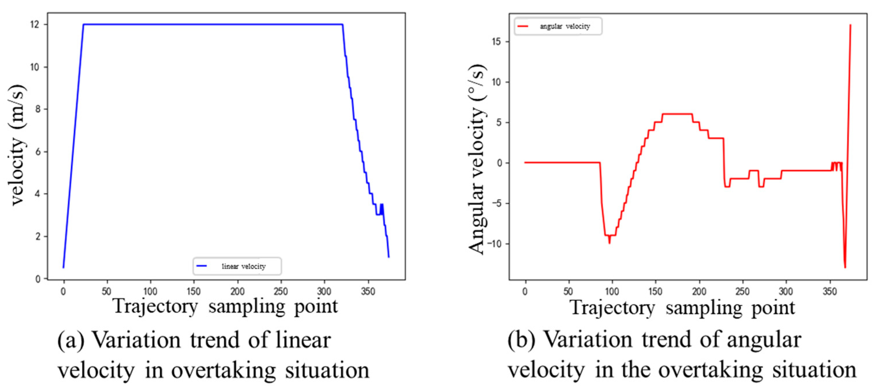
Figure 16 shows the variation trend of the linear velocity and angular velocity of the USV in the overtaking situation. Figure 16a shows the trend of linear speed change. During the whole process, the USV first sped up, then sailed at the maximum speed and uniform speed, and decelerated near the target point. Figure 16b shows the change trend of angular velocity and maintains the heading before overtaking. When overtaking, the USV has an obvious behavior turning port, the maximum turning rate reaches 10°/s, which is half of the maximum turning rate of the USV, and it moves towards the target point after overtaking.
Through the analysis, it can be seen that the algorithm proposed in this paper can guide the USV to avoid the target ship safely. Since the algorithm in this paper considers the constraints of the COLREGs, it has certain practical guiding significance.
4.3. Experimental Simulation in a Local Environment
In order to verify the feasibility of the algorithm in the environment with unknown obstacles, local path planning experiments are carried out.
- (1)
- Local path planning with dynamic obstructing ships and unknown static obstacles in the head-on situation.
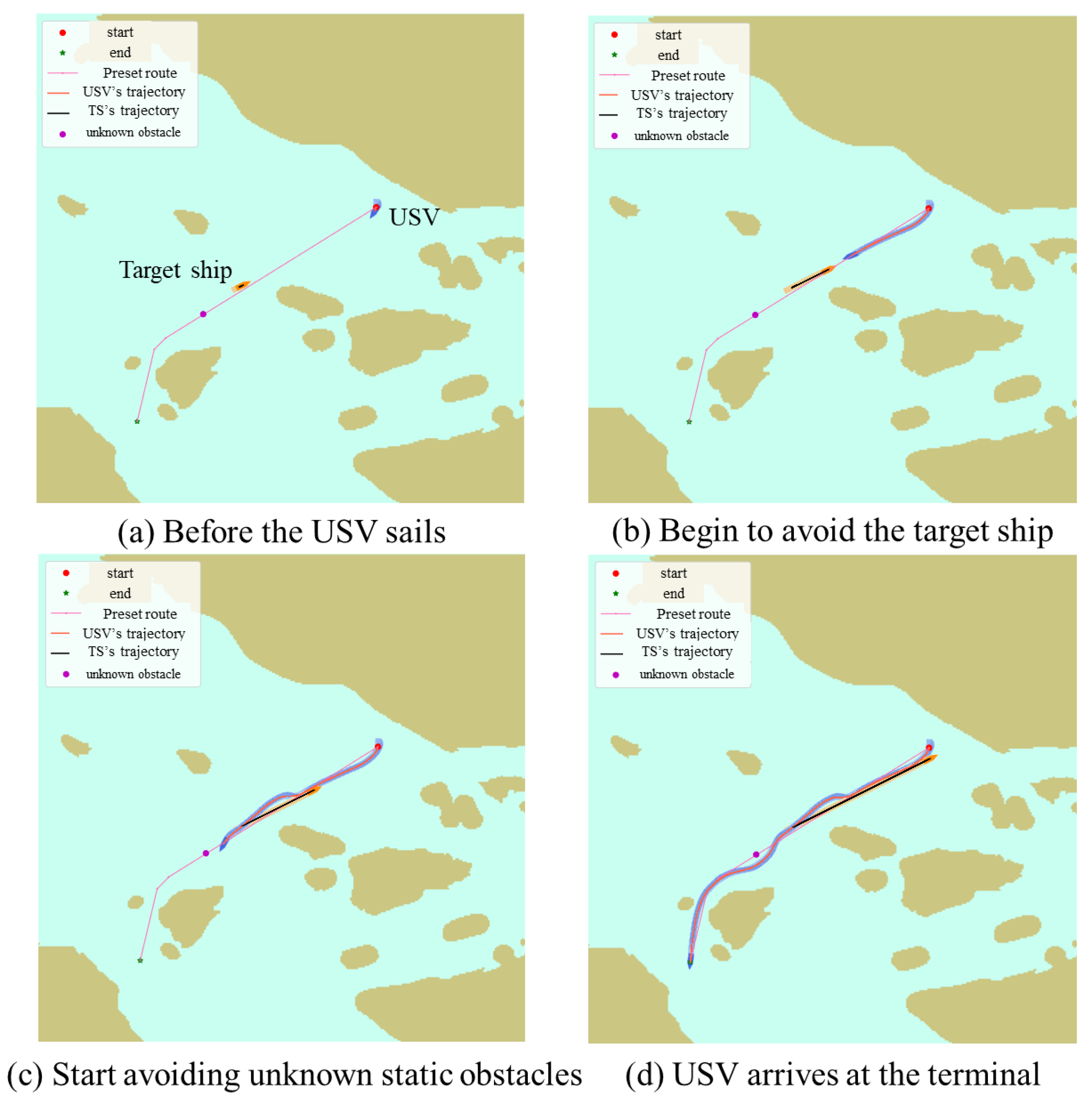
Figure 17 shows the local path planning process in head-on situations and unknown static obstacles. Figure 17a shows that when the USV starts sailing, the pink line represents the preset route from the starting point to the target point to guide the navigation of the USV, and the purple dotted area represents the unknown static obstacles that are not considered in the global path planning. Figure 17a shows that when there are unknown static obstacles on the route, sailing along the preset route will collide with the obstacles. Therefore, the USV needs to avoid unknown obstacles during actual navigation. The algorithm proposed in this paper adds constraints on unknown obstacles to the trajectory evaluation function, which can ensure that the USV avoids unknown static obstacles in the navigation environment. Figure 17b shows that the USV detects the dynamic ship in the situation of collision and starts to avoid the ship to the starboard. Figure 17c shows the moment when the USV has completed the collision avoidance process and the unknown static obstacle is detected when it continues to sail along the route. Figure 17d shows the time at which the USV reaches the target point. It can be seen from the figure that the USV’s navigation path can conduct collision avoidance operation between a single ship in a local environment and avoid unknown static obstacles.
- (2)
- Local path planning with dynamic obstructing ships and unknown static obstacles in crossing situations.
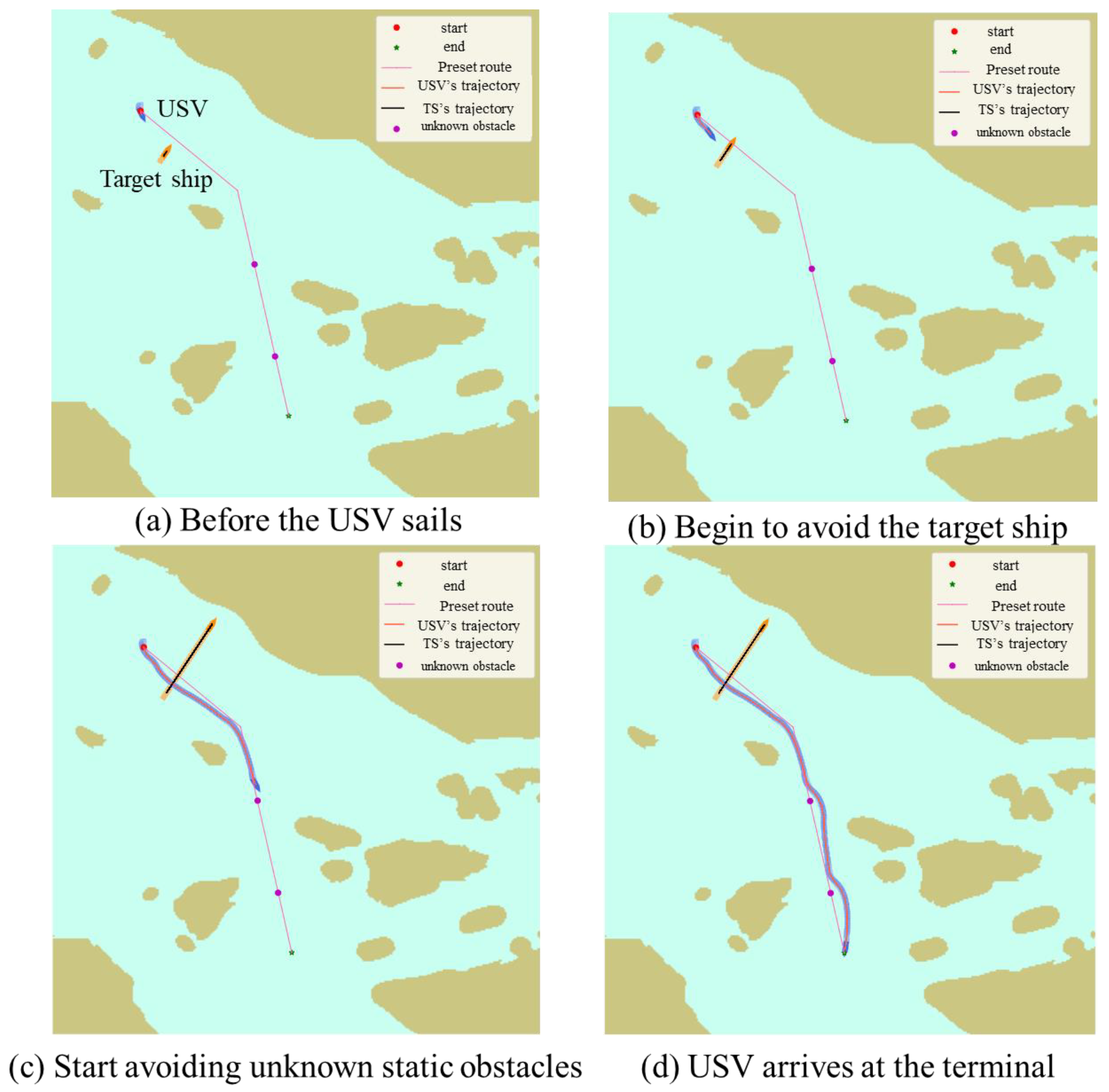
Figure 18 shows the local path planning process in crossing situations and unknown static obstacles. Figure 18a is when the USV is sailing, where the pink line represents the preset route that guides the unmanned ship from the starting point to the destination, and the two purple areas represent unknown static obstacles that are not considered in the global path planning. Figure 18b shows that the USV detects the dynamic ship in the crossing situation and starts to turn to the starboard to avoid collision. Figure 18c shows the moment when the USV completes the avoidance process in the crossing situation, detects an unknown static obstacle, and begins to avoid it. Figure 18d shows the time when the whole voyage is completed and the destination is reached. It can be seen from the figure that the navigation path of USV can avoid collision and unknown static obstacles under the crossing situation between a single ship in a local environment so as to ensure that the USV can sail smoothly to the destination.
- (3)
- Local path planning in the overtaking situation with dynamic obstructing ships and unknown static obstacles.
Figure 19 shows the local path planning process with an overtaking situation and two unknown static obstacles. Figure 18a is the state when the USV is sailing. Figure 19b shows the dynamic ship when the USV detects the situation of overtaking and starts to turn to starboard to overtake the ship. Figure 19c shows that the USV has completed the avoidance process in the overtaking situation. When it continues to sail, it detects an unknown static obstacle and begins to avoid the unknown static obstacle. Figure 19d shows the moment when the entire voyage is completed and the destination is reached.
- (4)
- Local path planning in three different situations containing dynamic obstructing ships and unknown static obstacles.
Figure 20 shows the path planning process of a multi-objective dynamic ship. At time T1, USV begins to sail. At time T2, USV starts sailing, forms a head-on situation with the target ship, and starts to turn to avoid. At time T3, the USV successfully evades and forms a crossing situation with the second target ship, and it begins to turn to the starboard to avoid. At time T4, USV has successfully evaded and returned to the preset route. Time T5 is when the USV finds the ship under the situation of overtaking and begins to implement the overtaking process. Time T6 is when the USV successfully reaches the target point.
Overall, the innovation of this article is that the hazard function is introduced as the evaluation function in global path planning. In local path planning, the distance function of static unknown obstacles is introduced. The computational complexity is not high, the speed of generating routes is improved, and the sensitivity of path planning is improved when facing unknown static obstacles. In local path planning, this method is suitable for simple collision avoidance situations. In more complex scenarios, the accuracy of route generation is reduced. Next, we will focus on studying the path planning of ships in complex scenarios.
5. Conclusions
In the global path planning, the constraints of water depth and safety distance are mainly considered. Using the Voronoi Field algorithm to set the safety distance constraints, combined with the A* algorithm, this paper realizes the smoothing process under different safety distances. Different routes are generated by setting different safety distance constraints such as 100 m, 200 m, 300 m, etc. Finally, the data collected in path planning are visualized, and the rationality and feasibility of the algorithm are analyzed.
This paper describes the problems of USV navigation based on global path planning, that is, insufficient consideration of unknown obstacles in the environment (dynamic and static obstacles). On this basis, this paper proposes a collision avoidance decision of USV based on the dynamic window method, including the USV kinematics model, trajectory sampling considering the constraints of the COLREGs, and the optimal trajectory evaluation method. Finally, the effectiveness and rationality of the method are proved by the simulation results of collision avoidance in different situations of ships and local path planning with unknown obstacles.
Author Contributions
Conceptualization, S.H. and J.Z.; Data curation, S.H.; Funding acquisition, S.H. and J.Z.; Investigation, S.T. and R.S.; Methodology, J.Z. and S.H. All authors have read and agreed to the published version of the manuscript.
Funding
This research is supported by the National Key Research and Development Program, China (Grant no. 2021YFC2801003) and the National Natural Science Foundation of China (Grant no. 51709167).
Institutional Review Board Statement
Not applicable.
Informed Consent Statement
Not applicable.
Data Availability Statement
Data sharing not applicable.
Conflicts of Interest
The authors declare no conflict of interest.
References
- Long, Y.; Liu, S.; Qiu, D.; Li, C.; Guo, X.; Shi, B.; AbouOmar, M.S. Local Path Planning with Multiple Constraints for USV Based on Improved Bacterial Foraging Optimization Algorithm. J. Mar. Sci. Eng. 2023, 11, 489. [Google Scholar] [CrossRef]
- Liu, X.; Li, Y.; Zhang, J.; Zheng, J.; Yang, C. Self-Adaptive Dynamic Obstacle Avoidance and Path Planning for USV under Complex Maritime Environment. IEEE Access 2019, 7, 114945–114954. [Google Scholar] [CrossRef]
- Liu, J.; Yan, X.; Liu, C.; Fan, A.; Ma, F. Developments and Applications of Green and Intelligent Inland Vessels in China. J. Mar. Sci. Eng. 2023, 11, 318. [Google Scholar] [CrossRef]
- Song, R.; Liu, Y.; Bucknall, R. Smoothed A* Algorithm for Practical Unmanned Surface Vehicle Path Planning. Appl. Ocean Res. 2019, 83, 9–20. [Google Scholar] [CrossRef]
- Han, X.; Zhang, X.; Zhang, H. Trajectory Planning of USV: On-Line Computation of the Double S Trajectory Based on Multi-Scale A* Algorithm with Reeds–Shepp Curves. J. Mar. Sci. Eng. 2023, 11, 153. [Google Scholar] [CrossRef]
- Zhao, J.; Yan, Z.; Chen, X.; Han, B.; Wu, S.; Ke, R. k-GCN-LSTM: A k-hop Graph Convolutional Network and Long–Short-Term Memory for ship speed prediction. Physica A 2022, 606, 128107. [Google Scholar] [CrossRef]
- Feng, Z.; Pan, Z.; Chen, W.; Liu, Y.; Leng, J. USV Application Scenario Expansion Based on Motion Control, Path Following and Velocity Planning. Machines 2022, 10, 310. [Google Scholar] [CrossRef]
- Xu, P.F.; Ding, Y.X.; Luo, J.C. Complete Coverage Path Planning of an Unmanned Surface Vehicle Based on a Complete Coverage Neural Network Algorithm. J. Mar. Sci. Eng. 2021, 9, 1163. [Google Scholar] [CrossRef]
- Ke, C.; Chen, H. Cooperative Path Planning for Air–Sea Heterogeneous Unmanned Vehicles Using Search-and-Tracking Mission. Ocean Eng. 2022, 262, 112020. [Google Scholar] [CrossRef]
- Zhang, J.; Zhang, D.; Yan, X.; Haugen, S.; Soares, C.G. A distributed anti-collision decision support formulation in multi-ship encounter situations under COLREGs. Ocean Eng. 2015, 105, 336–348. [Google Scholar] [CrossRef]
- Cai, M.; Zhang, J.; Zhang, D.; Yuan, X.; Soares, C.G. Collision risk analysis on ferry ships in Jiangsu Section of the Yangtze River based on AIS data. J. Reliab. Eng. Syst. Saf. 2021, 215, 107901. [Google Scholar] [CrossRef]
- Xu, H.; Hinostroza, M.A.; Guedes Soares, C. Modified Vector Field Path-Following Control System for an underactuated Autonomous surface ship model in the presence of static obstacles. J. Mar. Sci. Eng. 2021, 9, 652. [Google Scholar] [CrossRef]
- Zhang, J.; Zhang, H.; Liu, J.; Wu, D.; Soares, C.G. A Two-Stage Path Planning Algorithm Based on Rapid-Exploring Random Tree for Ships Navigating in Multi-Obstacle Water Areas Considering COLREGs. J. Mar. Sci. Eng. 2022, 10, 1441. [Google Scholar] [CrossRef]
- Zhang, Y.; Shi, G.; Liu, J. Dynamic Energy-Efficient Path Planning of Unmanned Surface Vehicle under Time-Varying Current and Wind. J. Mar. Sci. Eng. 2022, 10, 759. [Google Scholar] [CrossRef]
- Almoaili, E.; Kurdi, H. Path Planning Algorithm for Unmanned Ground Vehicles (UGVs) in Known Static Environments. Procedia Comput. Sci. 2020, 177, 57–63. [Google Scholar] [CrossRef]
- Wang, H.; Lu, L.; Li, T.; Wang, A. Multi-AUG Three-Dimensional Path Planning and Secure Cooperative Path Following under DoS Attacks. Ocean Eng. 2023, 274, 113864. [Google Scholar] [CrossRef]
- Jabbarpour, M.R.; Zarrabi, H.; Jung, J.J.; Kim, P. A Green Ant-Based Method for Path Planning of Unmanned Ground Vehicles. IEEE Access 2017, 5, 1820–1832. [Google Scholar] [CrossRef]
- Han, Z.; Chen, M.; Shao, S.; Wu, Q. Improved Artificial Bee Colony Algorithm-Based Path Planning of Unmanned Autonomous Helicopter Using Multi-Strategy Evolutionary Learning. Aerosp. Sci. Technol. 2022, 122, 107374. [Google Scholar] [CrossRef]
- Thoresen, M.; Nielsen, N.H.; Mathiassen, K.; Pettersen, K.Y. Path Planning for UGVs Based on Traversability Hybrid A*. IEEE Robot. Autom. Lett. 2021, 6, 1216–1223. [Google Scholar] [CrossRef]
- Shin, J.; Kwak, D.; Kwak, K. Model Predictive Path Planning for an Autonomous Ground Vehicle in Rough Terrain. Int. J. Control. Autom. Syst. 2021, 19, 2224–2237. [Google Scholar] [CrossRef]
- Chen, D.; Wang, Z.; Zhou, G.; Li, S. Path Planning and Energy Efficiency of Heterogeneous Mobile Robots Using Cuckoo–Beetle Swarm Search Algorithms with Applications in UGV Obstacle Avoidance. Sustainability 2022, 14, 15137. [Google Scholar] [CrossRef]
- Liang, C.; Zhang, X.; Watanabe, Y.; Deng, Y. Autonomous Collision Avoidance of Unmanned Surface Vehicles Based on Improved A Star And Minimum Course Alteration Algorithms. Appl. Ocean Res. 2021, 113, 102755. [Google Scholar] [CrossRef]
- Pasandi, L.; Hooshmand, M.; Rahbar, M. Modified A* Algorithm Integrated with Ant Colony Optimization for Multi-Objective Route-Finding; Case Study: Yazd. Appl. Soft Comput. 2021, 113, 107877. [Google Scholar] [CrossRef]
- Li, J.; Zhang, W.; Hu, Y.; Fu, S.; Liao, C.; Yu, W. RJA-Star Algorithm for UAV Path Planning Based on Improved R5DOS Model. Appl. Sci. 2023, 13, 1105. [Google Scholar] [CrossRef]
- Zou, A.; Wang, L.; Li, W.; Cai, J.; Wang, H.; Tan, T. Mobile Robot Path Planning Using Improved Mayfly Optimization Algorithm and Dynamic Window Approach. J. Supercomput. 2022, 79, 8340–8367. [Google Scholar] [CrossRef]
- Wang, N.; Xu, H. Dynamics-Constrained Global-Local Hybrid Path Planning of an Autonomous Surface Vehicle. IEEE Trans. Veh. Technol. 2020, 69, 6928–6942. [Google Scholar] [CrossRef]
- Han, S.; Wang, L.; Wang, Y.; He, H. A Dynamically Hybrid Path Planning for Unmanned Surface Vehicles Based on Non-Uniform Theta* and Improved Dynamic Windows Approach. Ocean Eng. 2022, 257, 111655. [Google Scholar] [CrossRef]
- Ji, X.; Feng, S.; Han, Q.; Yin, H.; Yu, S. Improvement and Fusion of A* Algorithm and Dynamic Window Approach Considering Complex Environmental Information. Arab. J. Sci. Eng. 2021, 46, 7445–7459. [Google Scholar] [CrossRef]
- Chi, W.; Ding, Z.; Wang, J.; Chen, G.; Sun, L. A Generalized Voronoi Diagram-Based Efficient Heuristic Path Planning Method for RRTs in Mobile Robots. IEEE Trans. Ind. Electron. 2022, 69, 4926–4937. [Google Scholar] [CrossRef]
- Chi, W.; Wang, J.; Ding, Z.; Chen, G.; Sun, L. A Reusable Generalized Voronoi Diagram-Based Feature Tree for Fast Robot Motion Planning in Trapped Environments. IEEE Sens. J. 2022, 22, 17615–17624. [Google Scholar] [CrossRef]
- Schoener, M.; Coyle, E.; Thompson, D. An Anytime Visibility–Voronoi Graph-Search Algorithm for Generating Robust and Feasible Unmanned Surface Vehicle Paths. Auton. Robots 2022, 46, 911–927. [Google Scholar] [CrossRef]
Figure 1.
The flowchart of global and local path planning.

Figure 2.
Coordinate transformation diagram.

Figure 3.
Kinematics Model of USV.

Figure 4.
Dynamic ship risk detection.

Figure 5.
Global path planning results under different safety distance constraints.

Figure 6.
Comparison of path smoothing effects under different safety distance constraints. The meaning of different colored lines is same as Figure 5.
Figure 6.
Comparison of path smoothing effects under different safety distance constraints. The meaning of different colored lines is same as Figure 5.

Figure 7.
The distance between path nodes and obstacles under different safety distances.

Figure 8.
Simulation results of collision avoidance in a head-on situation.

Figure 9.
The heading change curve and the DCPA diagram in the head-on situation.

Figure 10.
Trend diagram of speed change in a head-on situation.

Figure 11.
Simulation results of collision avoidance in a crossing situation.

Figure 12.
The course change curve and the DCPA diagram in the crossing situation.

Figure 13.
Velocity variation trend diagram in a crossing situation.

Figure 14.
Simulation results of collision avoidance in an overtaking situation.

Figure 15.
The course change curve and the DCPA diagram in the overtaking situation.

Figure 16.
Velocity variation trend diagram in the situation of overtaking.

Figure 17.
Partial path planning process in the head-on situation.

Figure 18.
Local path planning process in the crossing situation.

Figure 19.
Local path planning process in an overtaking situation.

Figure 20.
Path planning process of a multi-objective dynamic ship.


Table 1.
Comparison table of rendering colors for different environmental information of the chart.
| Chart Environmental Information | Color | Red | Green | Blue |
|---|---|---|---|---|
| Areas with a water depth of 30–50 m |  | 216 | 244 | 225 |
| Areas with a water depth of 10–20 m |  | 185 | 225 | 222 |
| Areas with a water depth of 5 m |  | 152 | 211 | 237 |
| Areas with a water depth of 1–2 m |  | 123 | 193 | 241 |
| shoal |  | 115 | 185 | 142 |
| land |  | 203 | 199 | 131 |
Table 2.
Comparison of path planning results under different safety distances.
| Safe Distance/m | Original Path Length/km | Optimized Path Length/km | Number of Nodes | Number of Optimized Nodes |
|---|---|---|---|---|
| D = 0 | 12.08 | - | 398 | - |
| D = 100 | 12.14 | 11.32 | 402 | 5 |
| D = 200 | 12.23 | 11.38 | 409 | 6 |
| D = 300 | 12.30 | 11.48 | 414 | 6 |
Table 3.
Simulation parameters of USV.
| Parameter | Linear Velocity | Angular Velocity |
|---|---|---|
| minimum value | 0 m/s | −20°/s |
| maximum value | 5 m/s | 20°/s |
| maximum acceleration | 2 m/s2 | 5°/s2 |
| sampling interval | 0.2 m/s | 1°/s |
Table 4.
Simulation parameters of USV.
| Predicted Time/s | Safe Distance/m | ||||
|---|---|---|---|---|---|
| 0.02 | 0.4 | 0.2 | 0.2 | 5 | 50 |
Disclaimer/Publisher’s Note: The statements, opinions and data contained in all publications are solely those of the individual author(s) and contributor(s) and not of MDPI and/or the editor(s). MDPI and/or the editor(s) disclaim responsibility for any injury to people or property resulting from any ideas, methods, instructions or products referred to in the content. |
© 2023 by the authors. Licensee MDPI, Basel, Switzerland. This article is an open access article distributed under the terms and conditions of the Creative Commons Attribution (CC BY) license (https://creativecommons.org/licenses/by/4.0/).
Share and Cite
MDPI and ACS Style
Hu, S.; Tian, S.; Zhao, J.; Shen, R. Path Planning of an Unmanned Surface Vessel Based on the Improved A-Star and Dynamic Window Method. J. Mar. Sci. Eng. 2023, 11, 1060. https://doi.org/10.3390/jmse11051060
AMA Style
Hu S, Tian S, Zhao J, Shen R. Path Planning of an Unmanned Surface Vessel Based on the Improved A-Star and Dynamic Window Method. Journal of Marine Science and Engineering. 2023; 11(5):1060. https://doi.org/10.3390/jmse11051060
Chicago/Turabian StyleHu, Shunan, Shenpeng Tian, Jiansen Zhao, and Ruiqi Shen. 2023. "Path Planning of an Unmanned Surface Vessel Based on the Improved A-Star and Dynamic Window Method" Journal of Marine Science and Engineering 11, no. 5: 1060. https://doi.org/10.3390/jmse11051060
Note that from the first issue of 2016, this journal uses article numbers instead of page numbers. See further details here.