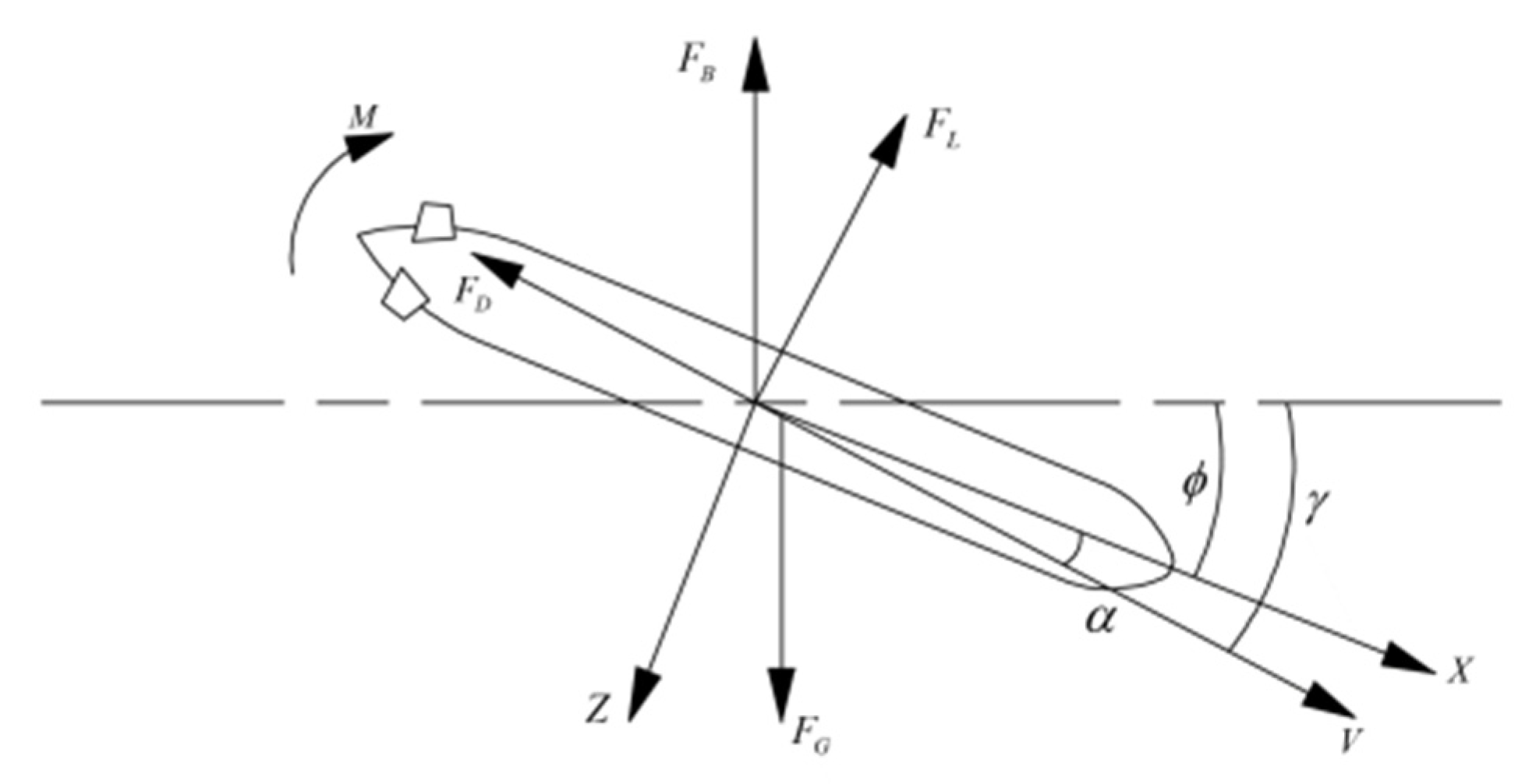
Figure 1.
The force analysis of the AUG from the perspective of the vertical section.
Figure 1.
The force analysis of the AUG from the perspective of the vertical section.
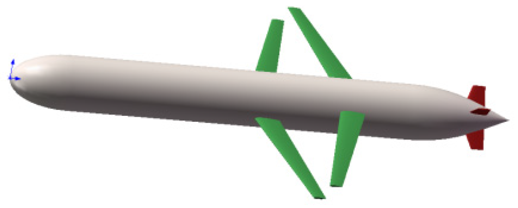
Figure 2.
Concept model for the hydrodynamic shape based on the AUG Sea-wing.
Figure 2.
Concept model for the hydrodynamic shape based on the AUG Sea-wing.
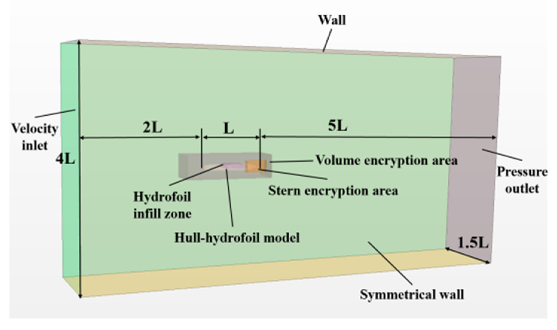
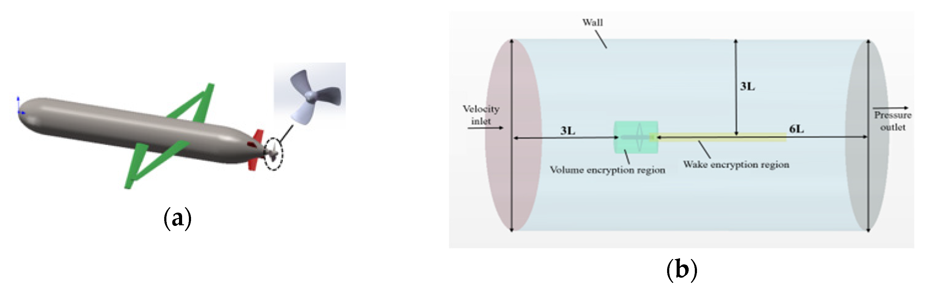
Figure 3.
Numerical tank with the boundary conditions.
Figure 3.
Numerical tank with the boundary conditions.
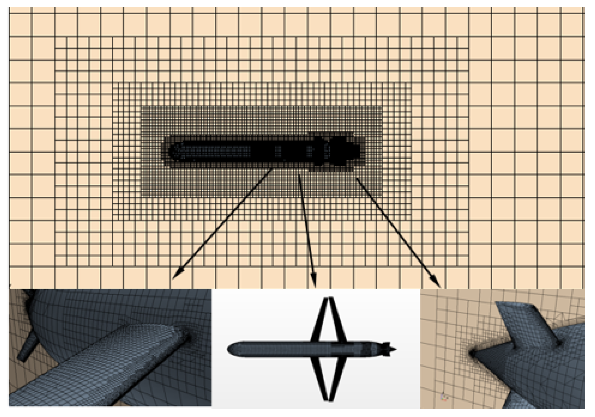
Figure 4.
Mesh of the AUG.
Figure 4.
Mesh of the AUG.
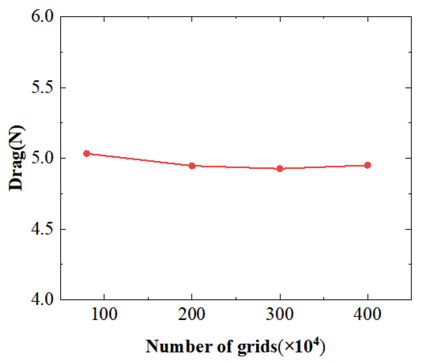
Figure 5.
Mesh independence of the AUG in terms of drag.
Figure 5.
Mesh independence of the AUG in terms of drag.
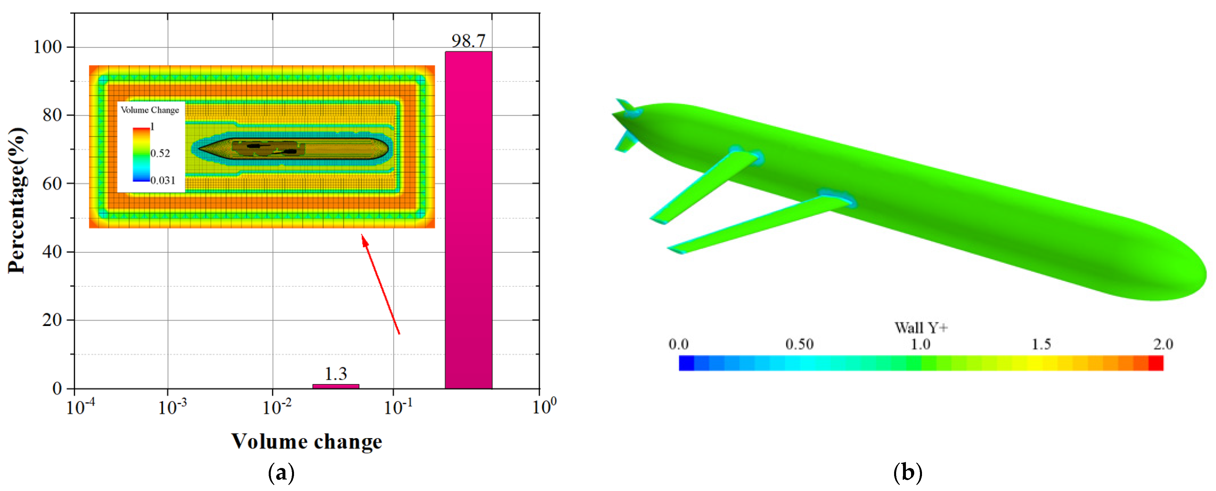
Figure 6.
Mesh quality evaluation by the volume change method (a) and y+ distribution (b) (mesh base size 0.25 m).
Figure 6.
Mesh quality evaluation by the volume change method (a) and y+ distribution (b) (mesh base size 0.25 m).
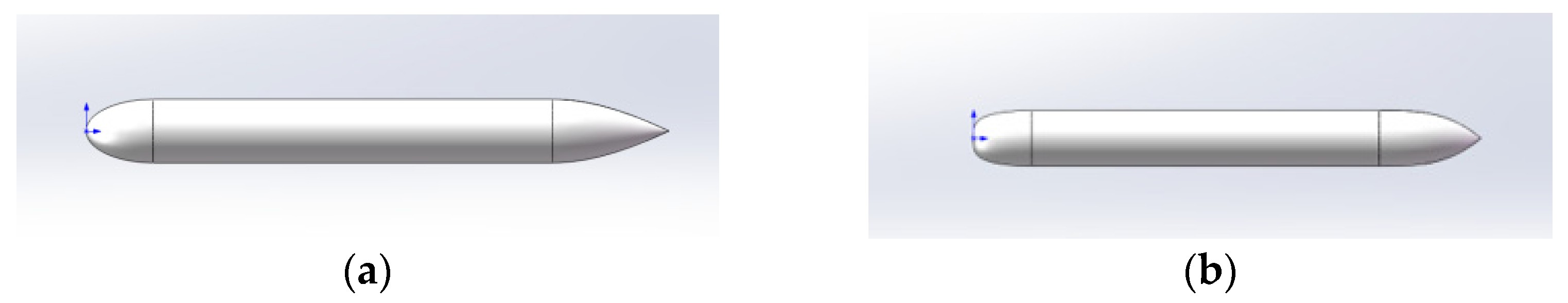
Figure 7.
Three-dimensional sketch of two kinds of hull models, the model with p = 2; θ = 25° (a) and the model with p = 4; θ = 40° (b).
Figure 7.
Three-dimensional sketch of two kinds of hull models, the model with p = 2; θ = 25° (a) and the model with p = 4; θ = 40° (b).
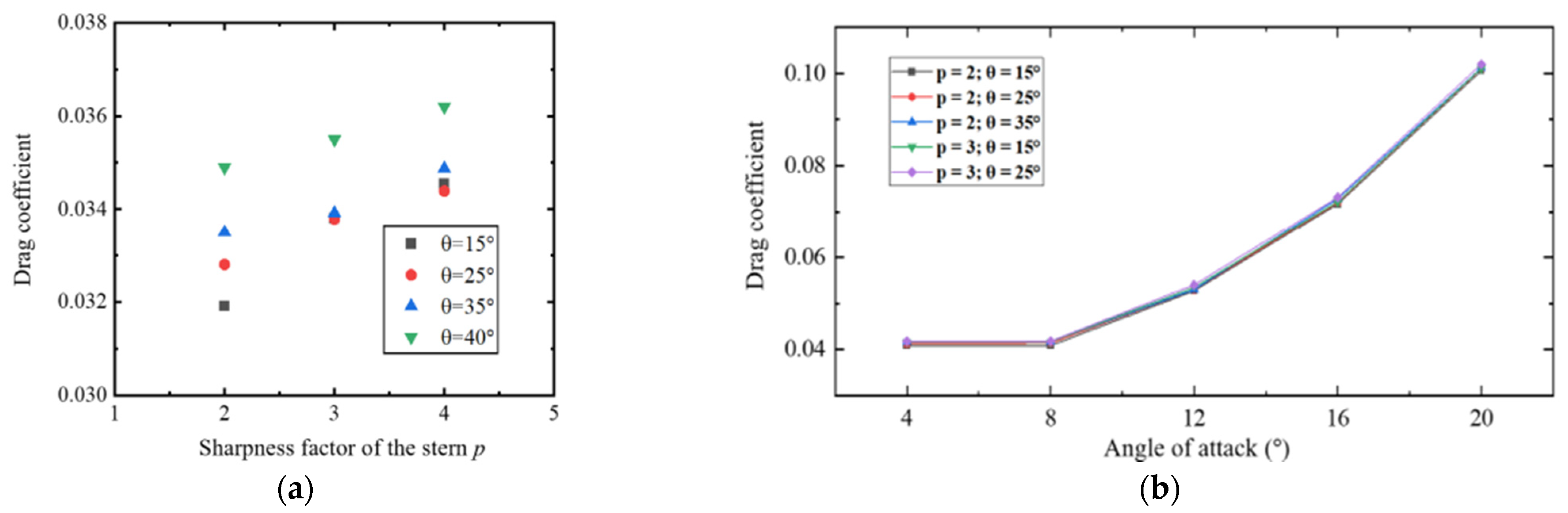
Figure 8.
Drag coefficient of different hull models in terms of straight-line motion (a) and oblique motion (b) with different angles of attack.
Figure 8.
Drag coefficient of different hull models in terms of straight-line motion (a) and oblique motion (b) with different angles of attack.
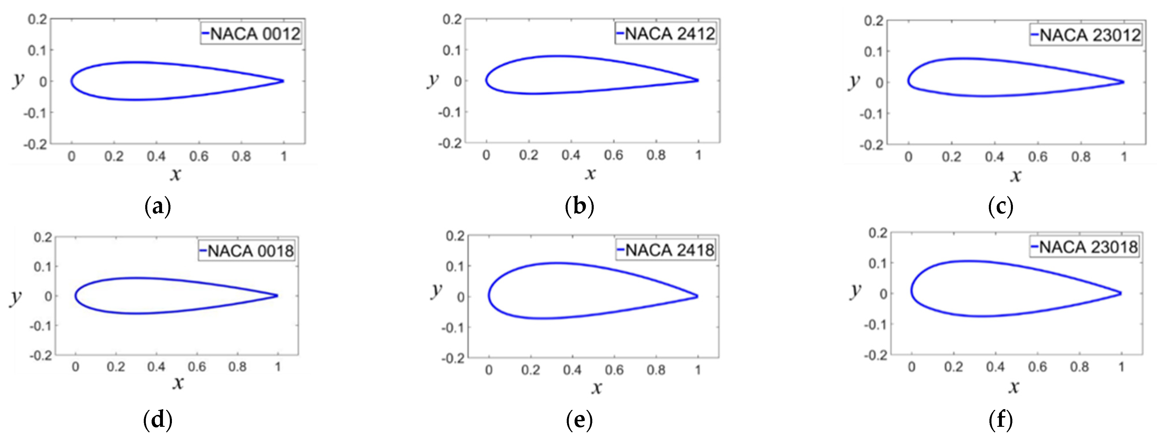
Figure 9.
Geometric sketch of the six different airfoil profiles: NACA0012 (a), NACA2412 (b), NACA23012 (c), NACA0018 (d), NACA2418 (e), and NACA23018 (f).
Figure 9.
Geometric sketch of the six different airfoil profiles: NACA0012 (a), NACA2412 (b), NACA23012 (c), NACA0018 (d), NACA2418 (e), and NACA23018 (f).
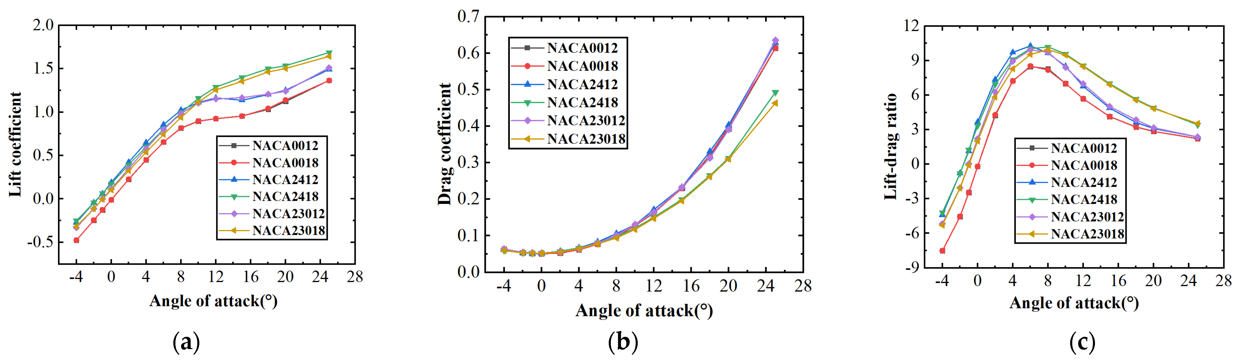
Figure 10.
Hydrodynamic calculation results of the rhomboid wing with different types of airfoils, lift coefficient (a), drag coefficient (b), and lift–drag ratio (c).
Figure 10.
Hydrodynamic calculation results of the rhomboid wing with different types of airfoils, lift coefficient (a), drag coefficient (b), and lift–drag ratio (c).
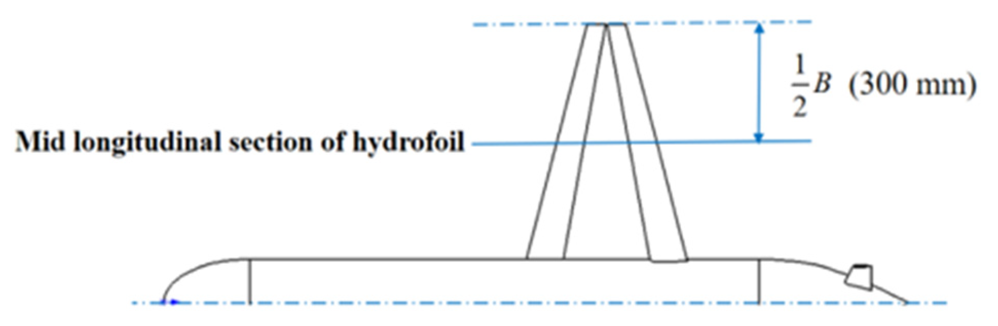
Figure 11.
The hydrofoil profile in the longitudinal section in the center plane.
Figure 11.
The hydrofoil profile in the longitudinal section in the center plane.
Figure 12.
Velocity and streamline distribution in the middle longitudinal section of the wing at different angles of attack: α = 0° (a), α = 6° (b), α = 8° (c), α = 12° (d), α = 15° (e), α = 20° (f) (in each sub-image, left: NACA2412; right: NACA2418).
Figure 12.
Velocity and streamline distribution in the middle longitudinal section of the wing at different angles of attack: α = 0° (a), α = 6° (b), α = 8° (c), α = 12° (d), α = 15° (e), α = 20° (f) (in each sub-image, left: NACA2412; right: NACA2418).
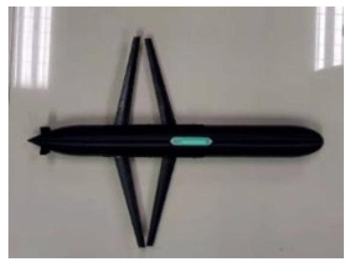
Figure 13.
The S-AUG model.
Figure 13.
The S-AUG model.
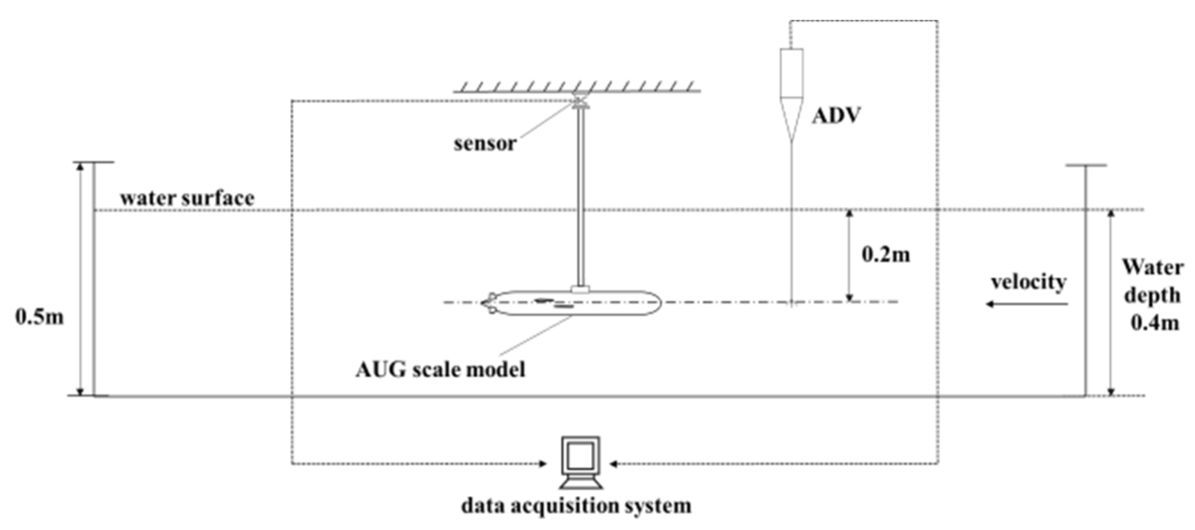
Figure 14.
Schematic diagram of the test system.
Figure 14.
Schematic diagram of the test system.
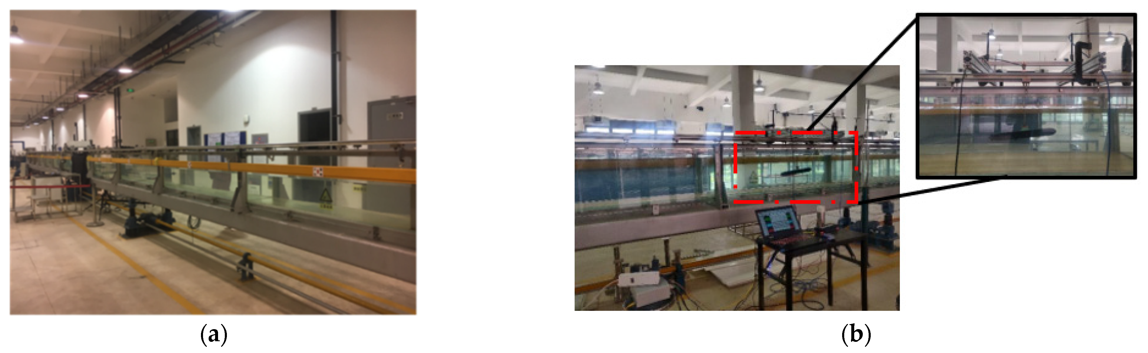
Figure 15.
Test scene from a whole view (a) and a side view (b).
Figure 15.
Test scene from a whole view (a) and a side view (b).
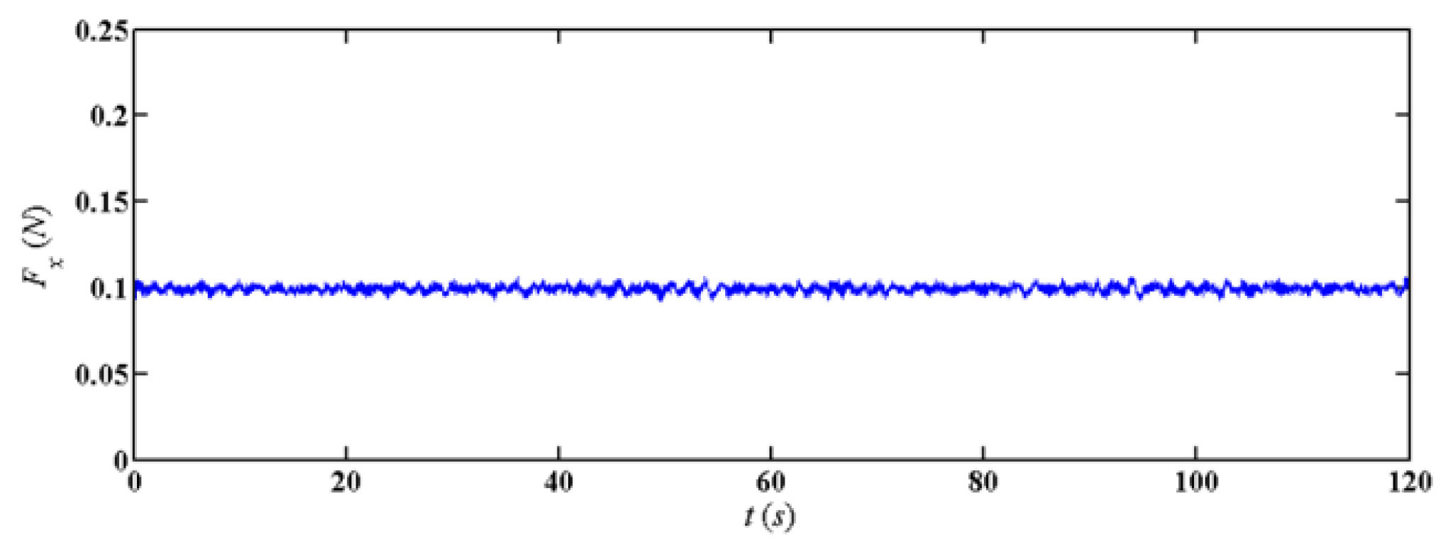
Figure 16.
Measurement results after smoothing filtering (α = 0°).
Figure 16.
Measurement results after smoothing filtering (α = 0°).
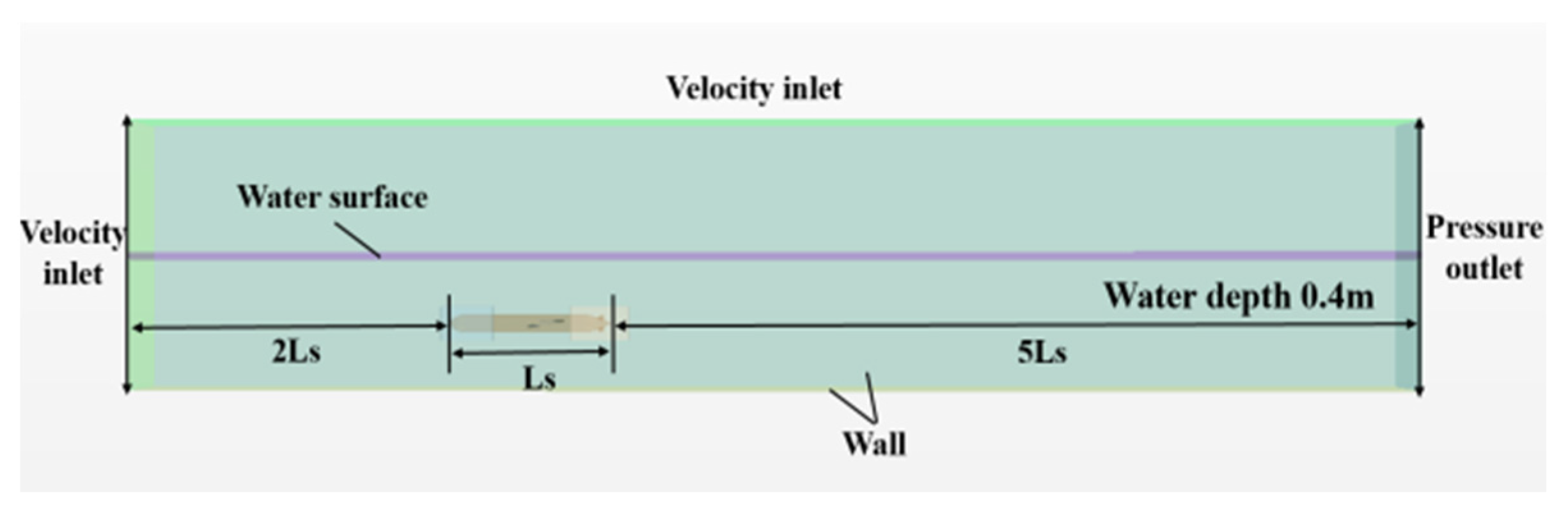
Figure 17.
Numerical towing tank with the boundary conditions.
Figure 17.
Numerical towing tank with the boundary conditions.
Figure 18.
The experimental and simulation results (a) and error assessment (b) of S-AUG (V = 0.4 m/s; Error = (EFD − CFD)/CFD × 100%).
Figure 18.
The experimental and simulation results (a) and error assessment (b) of S-AUG (V = 0.4 m/s; Error = (EFD − CFD)/CFD × 100%).
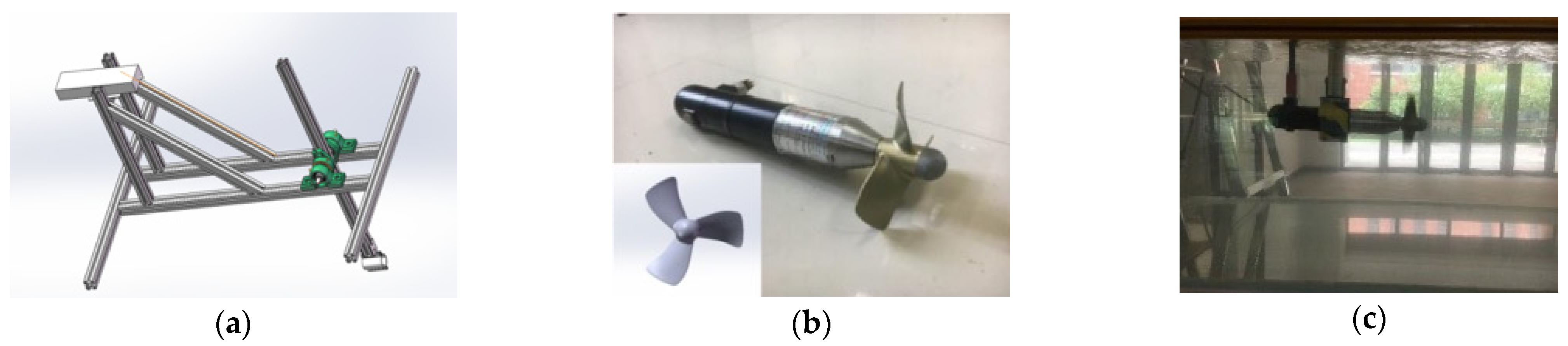
Figure 19.
The equipment of propeller thrust test, the thrust test bracket (a), Whale715 propeller with the electric motor (b), and the combination of the test system (c).
Figure 19.
The equipment of propeller thrust test, the thrust test bracket (a), Whale715 propeller with the electric motor (b), and the combination of the test system (c).
Figure 20.
Propeller test and simulation results (a) and the error assessment of the simulation results (b).
Figure 20.
Propeller test and simulation results (a) and the error assessment of the simulation results (b).
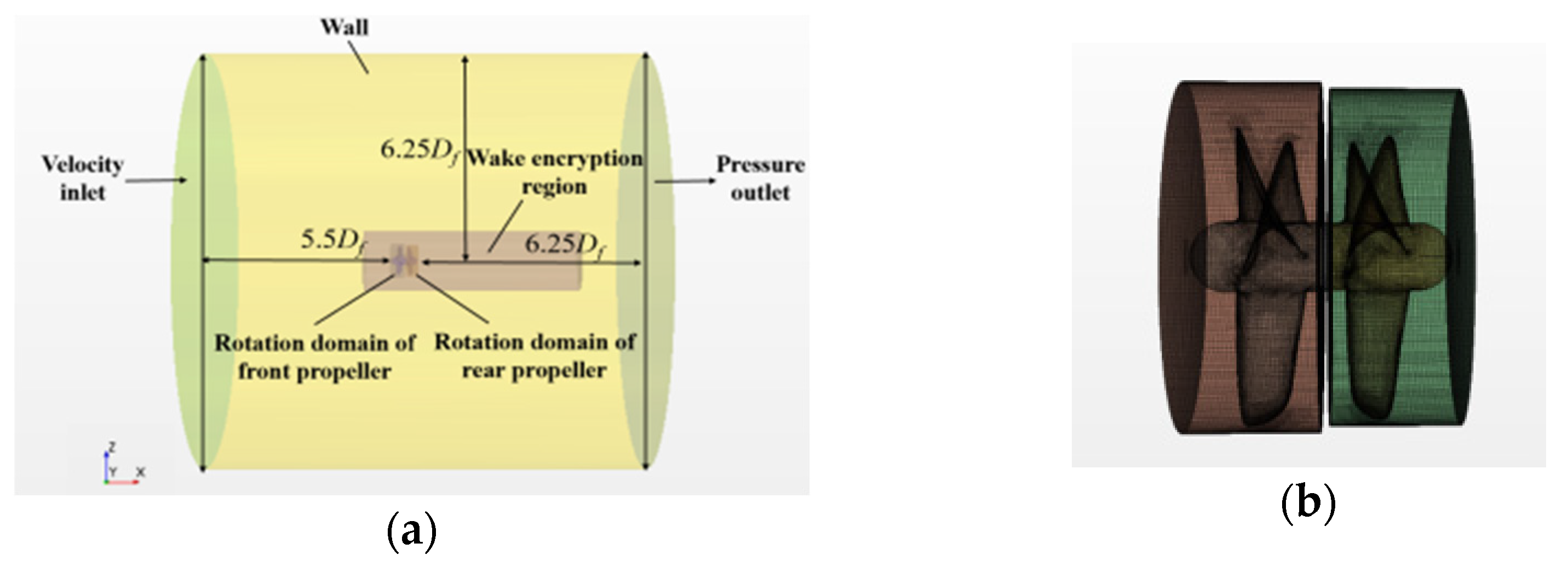
Figure 21.
Calculation domain (a) and mesh (b) of the CRP.
Figure 21.
Calculation domain (a) and mesh (b) of the CRP.
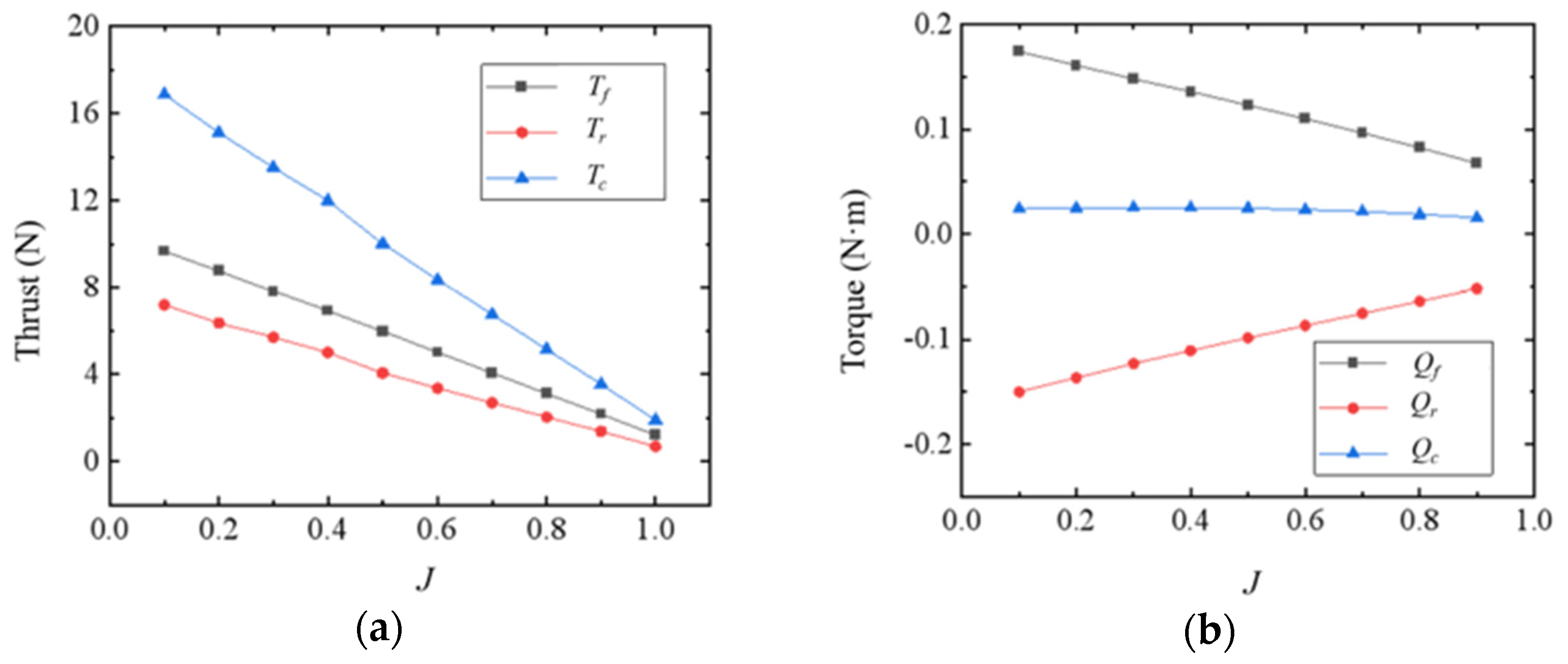
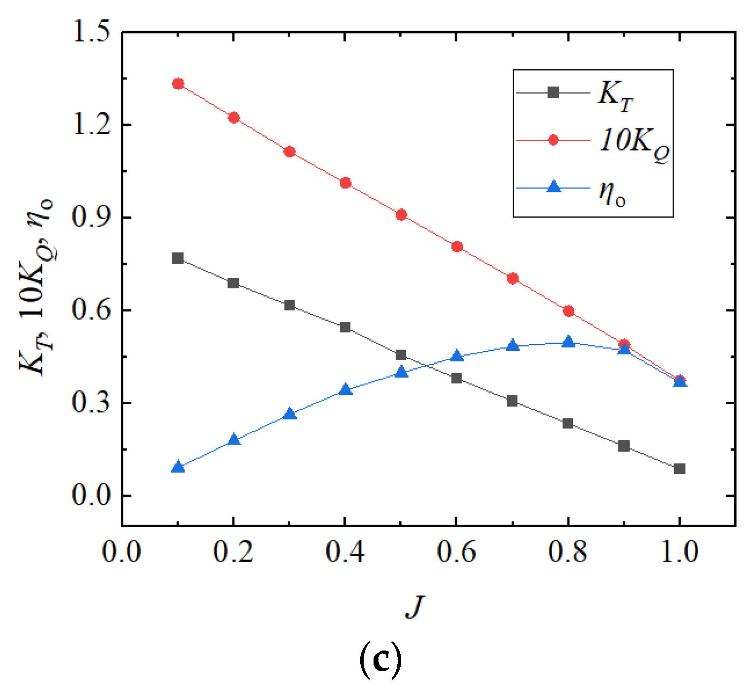
Figure 22.
The open water performance of the CRP in terms of the thrust output (a), the torque output (b), and the dimensionless K-J parameters (c) (subscript f: front propeller; r: rear propeller; c: counter rotating propeller).
Figure 22.
The open water performance of the CRP in terms of the thrust output (a), the torque output (b), and the dimensionless K-J parameters (c) (subscript f: front propeller; r: rear propeller; c: counter rotating propeller).
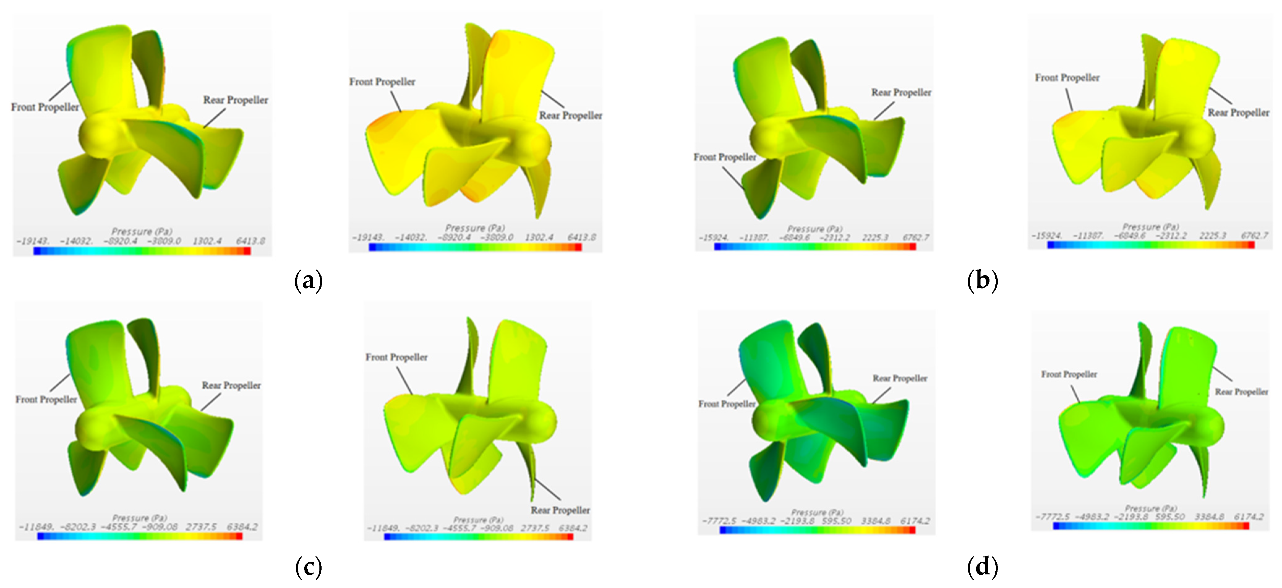
Figure 23.
Pressure distribution on the CRP surfaces with different advance coefficients, J = 0.1 (a), J = 0.3 (b), J = 0.5 (c), and J = 0.7 (d).
Figure 23.
Pressure distribution on the CRP surfaces with different advance coefficients, J = 0.1 (a), J = 0.3 (b), J = 0.5 (c), and J = 0.7 (d).
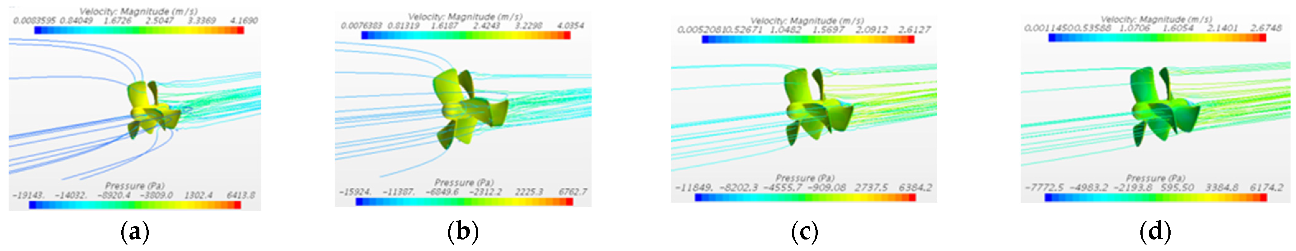
Figure 24.
Wake streamline distribution of CRP, J = 0.1 (a), J = 0.3 (b), J = 0.5 (c), and J = 0.7 (d).
Figure 24.
Wake streamline distribution of CRP, J = 0.1 (a), J = 0.3 (b), J = 0.5 (c), and J = 0.7 (d).
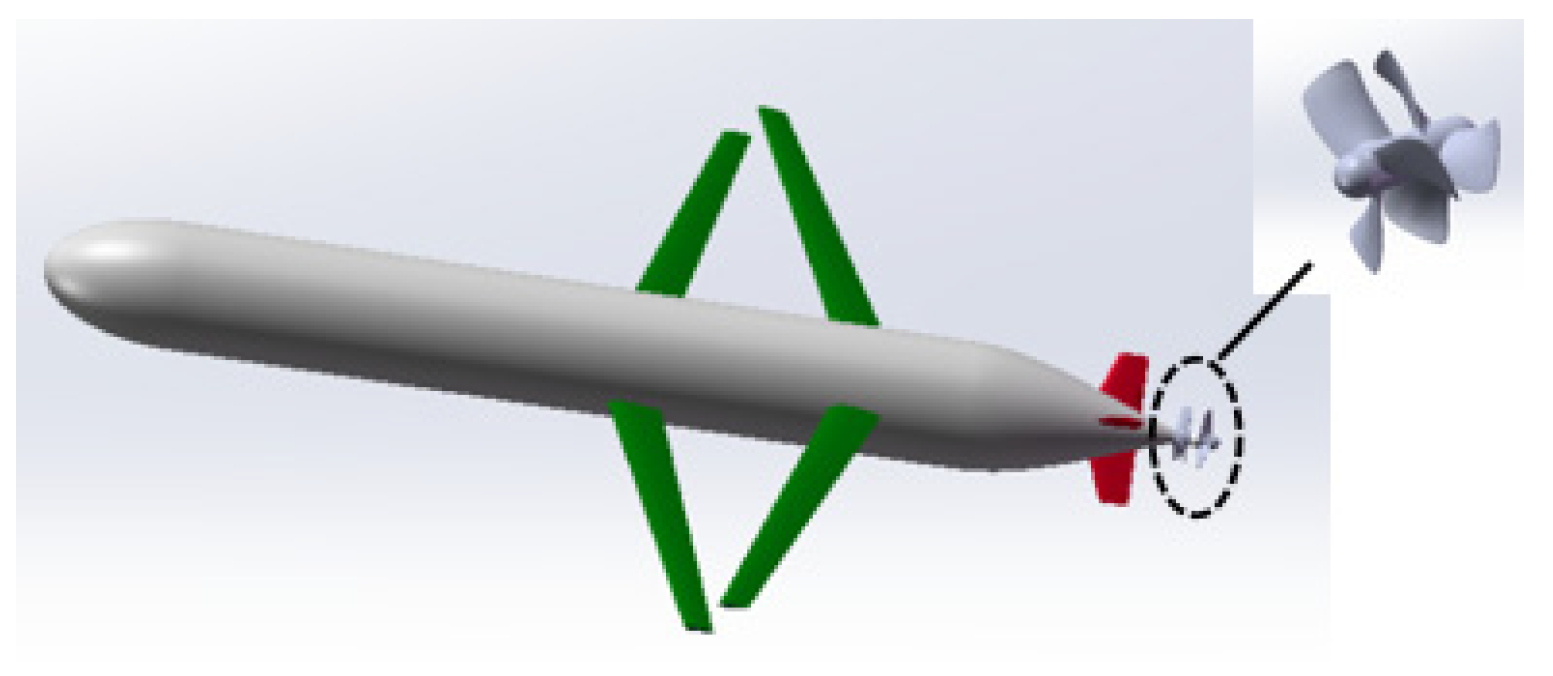
Figure 25.
The 3D model (a) and the calculation domain (b) of the hybrid-driven AUG with the single propeller.
Figure 25.
The 3D model (a) and the calculation domain (b) of the hybrid-driven AUG with the single propeller.
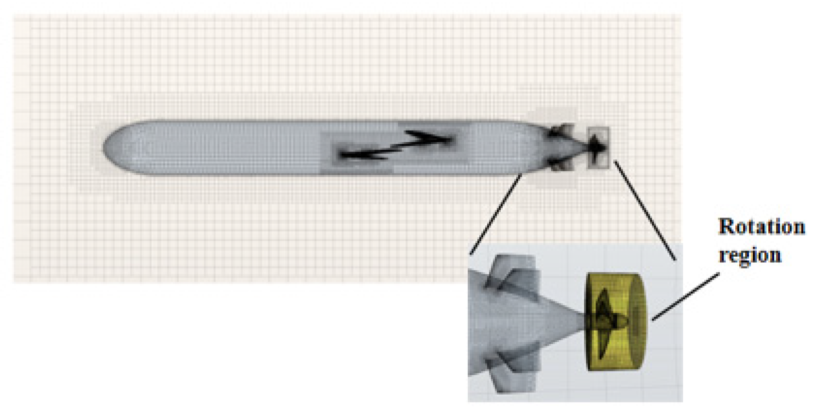
Figure 26.
Mesh of the hybrid-driven AUG with the single propeller.
Figure 26.
Mesh of the hybrid-driven AUG with the single propeller.
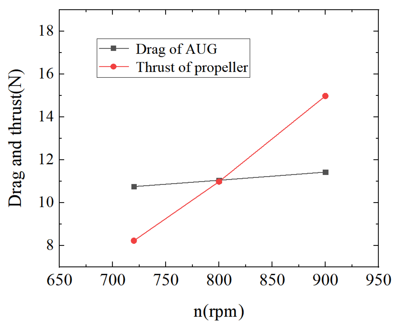
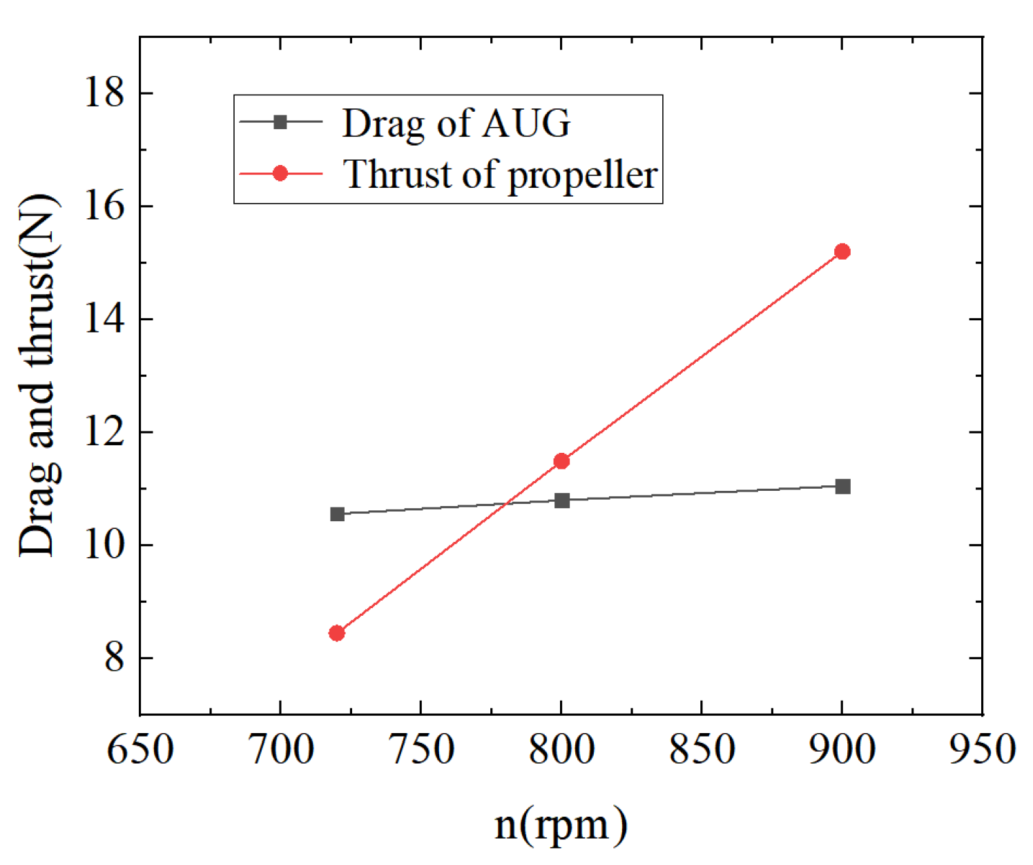
Figure 27.
Self-propulsion results of the hybrid-driven AUG with the single propeller.
Figure 27.
Self-propulsion results of the hybrid-driven AUG with the single propeller.
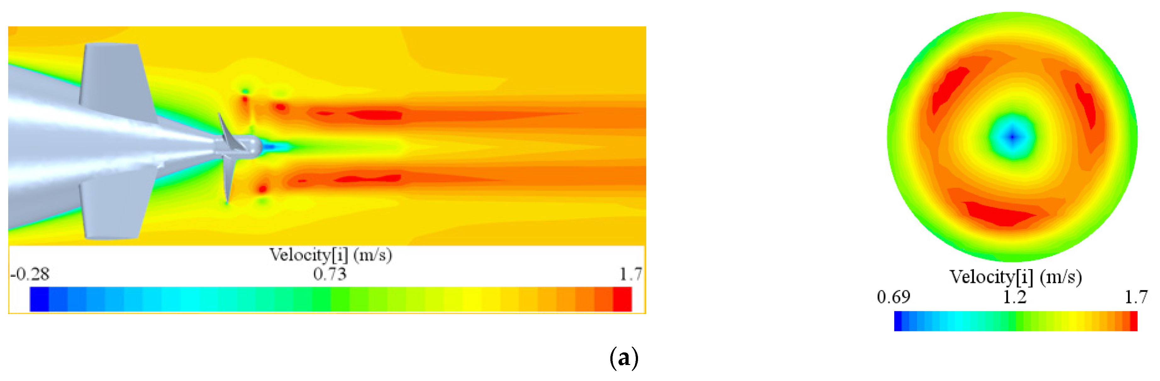
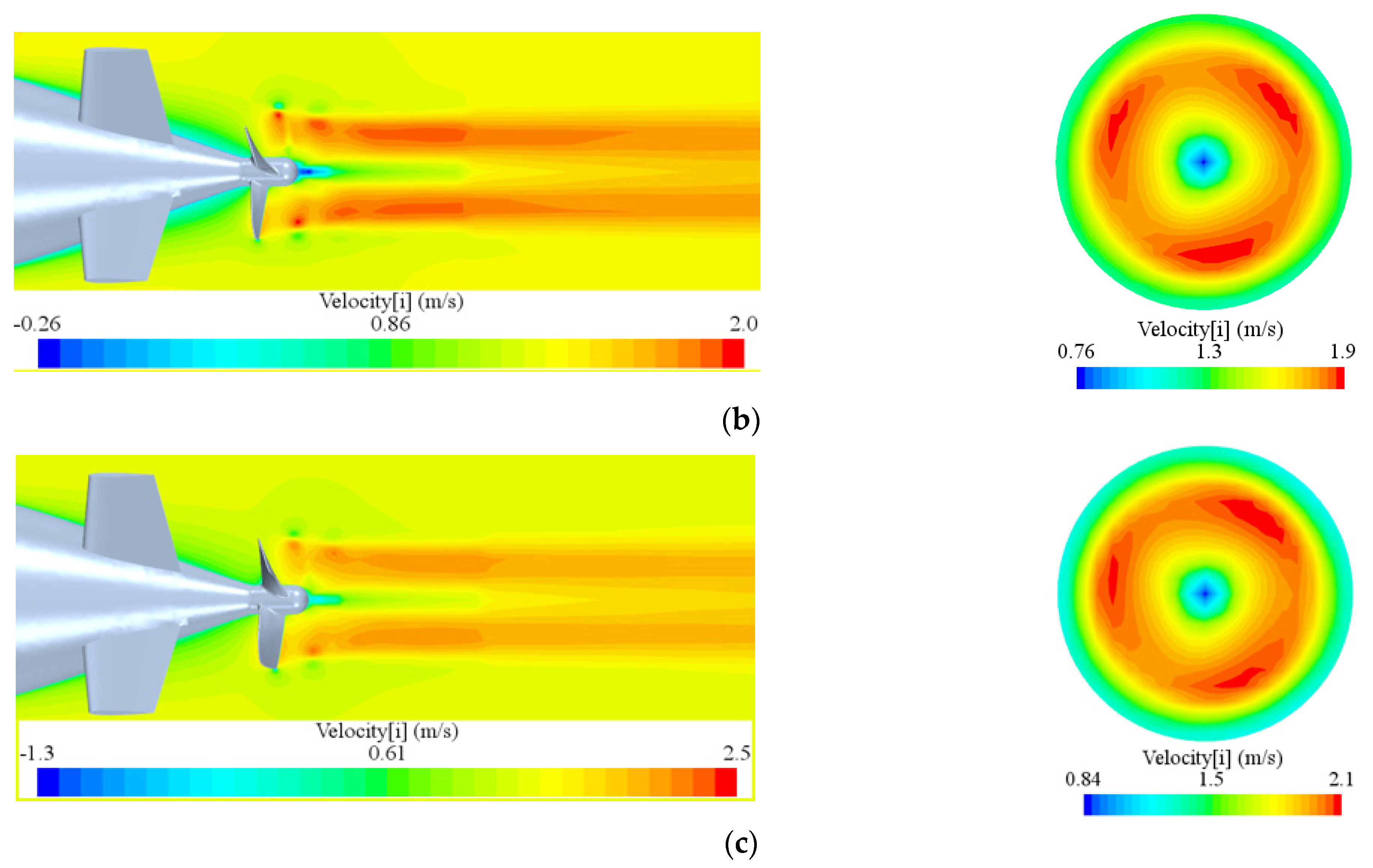
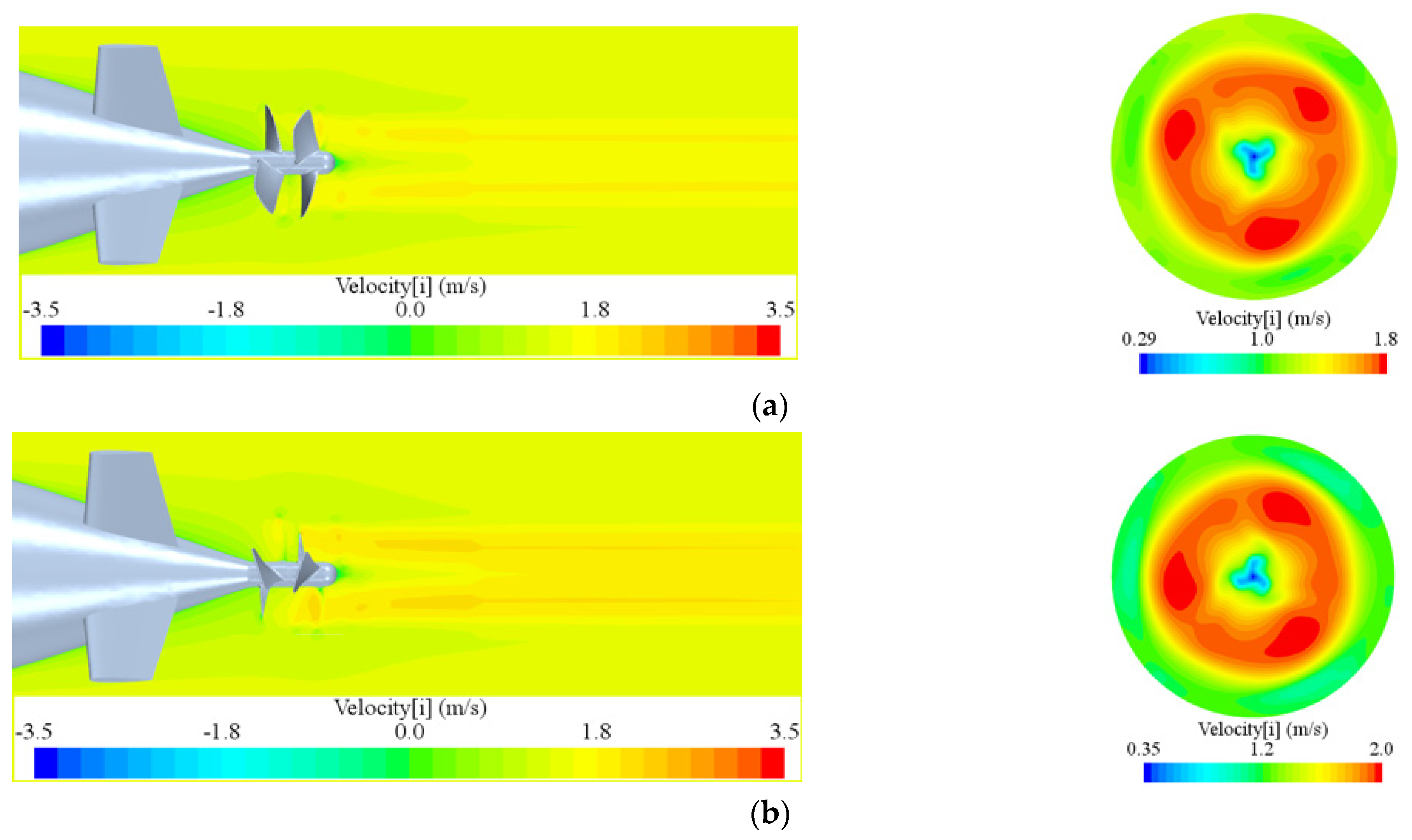
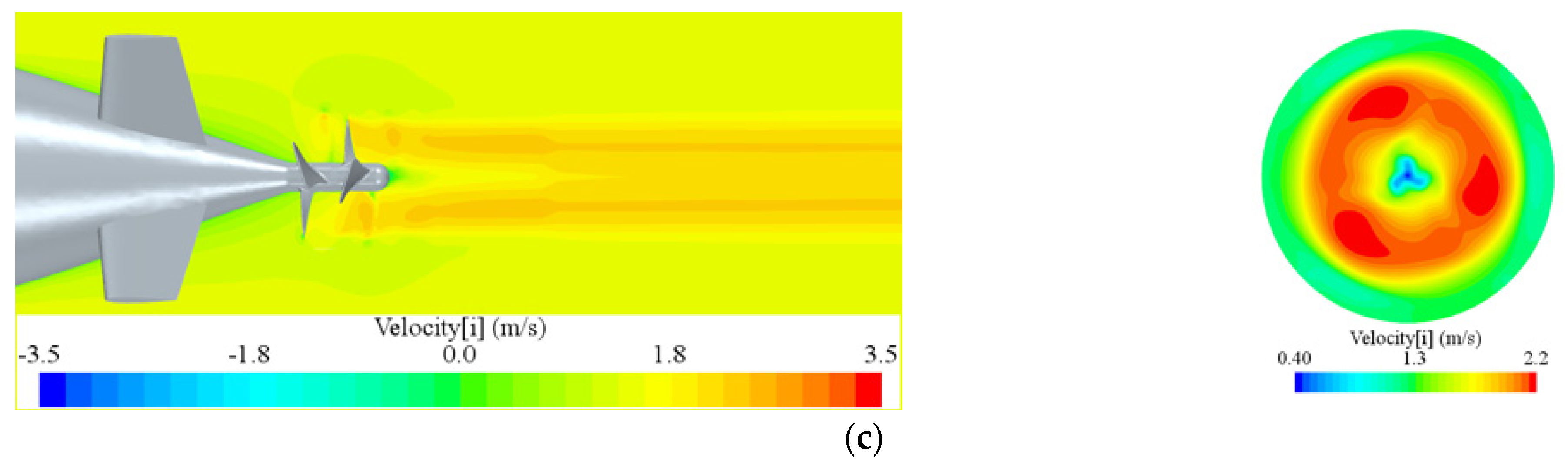
Figure 28.
Velocity distribution of the hybrid-driven AUG with the single propeller with propeller rotation speeds of 720 rpm (a), 800 rpm (b), and 900 rpm (c).
Figure 28.
Velocity distribution of the hybrid-driven AUG with the single propeller with propeller rotation speeds of 720 rpm (a), 800 rpm (b), and 900 rpm (c).
Figure 29.
Model of the AUG with the CRP.
Figure 29.
Model of the AUG with the CRP.
Figure 30.
Self-propulsion simulation results of the AUG with the CRP.
Figure 30.
Self-propulsion simulation results of the AUG with the CRP.
Figure 31.
Velocity distribution of the hybrid-driven AUG with the CRP at rotation speeds of 720 rpm (a), 800 rpm (b), and 900 rpm (c) including the sideview of the wake and the axial velocity plane 0.085Da downstream of the rear propeller disk.
Figure 31.
Velocity distribution of the hybrid-driven AUG with the CRP at rotation speeds of 720 rpm (a), 800 rpm (b), and 900 rpm (c) including the sideview of the wake and the axial velocity plane 0.085Da downstream of the rear propeller disk.
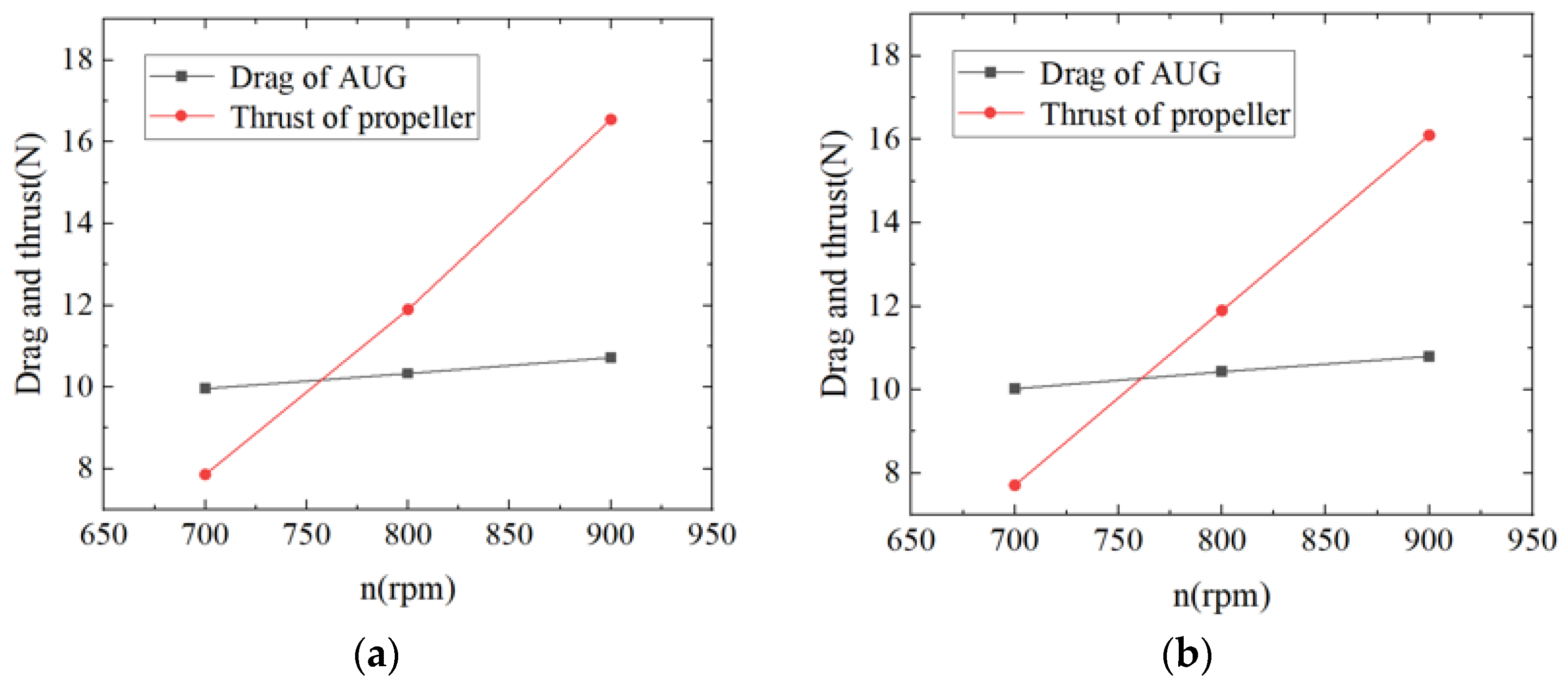
Figure 32.
The self-propulsion simulation results of the hybrid-driven AUGs with different hull lines, (p = 2; θ = 25°; NACA2418) (a) and (p = 3; θ = 25°; NACA2418) (b).
Figure 32.
The self-propulsion simulation results of the hybrid-driven AUGs with different hull lines, (p = 2; θ = 25°; NACA2418) (a) and (p = 3; θ = 25°; NACA2418) (b).
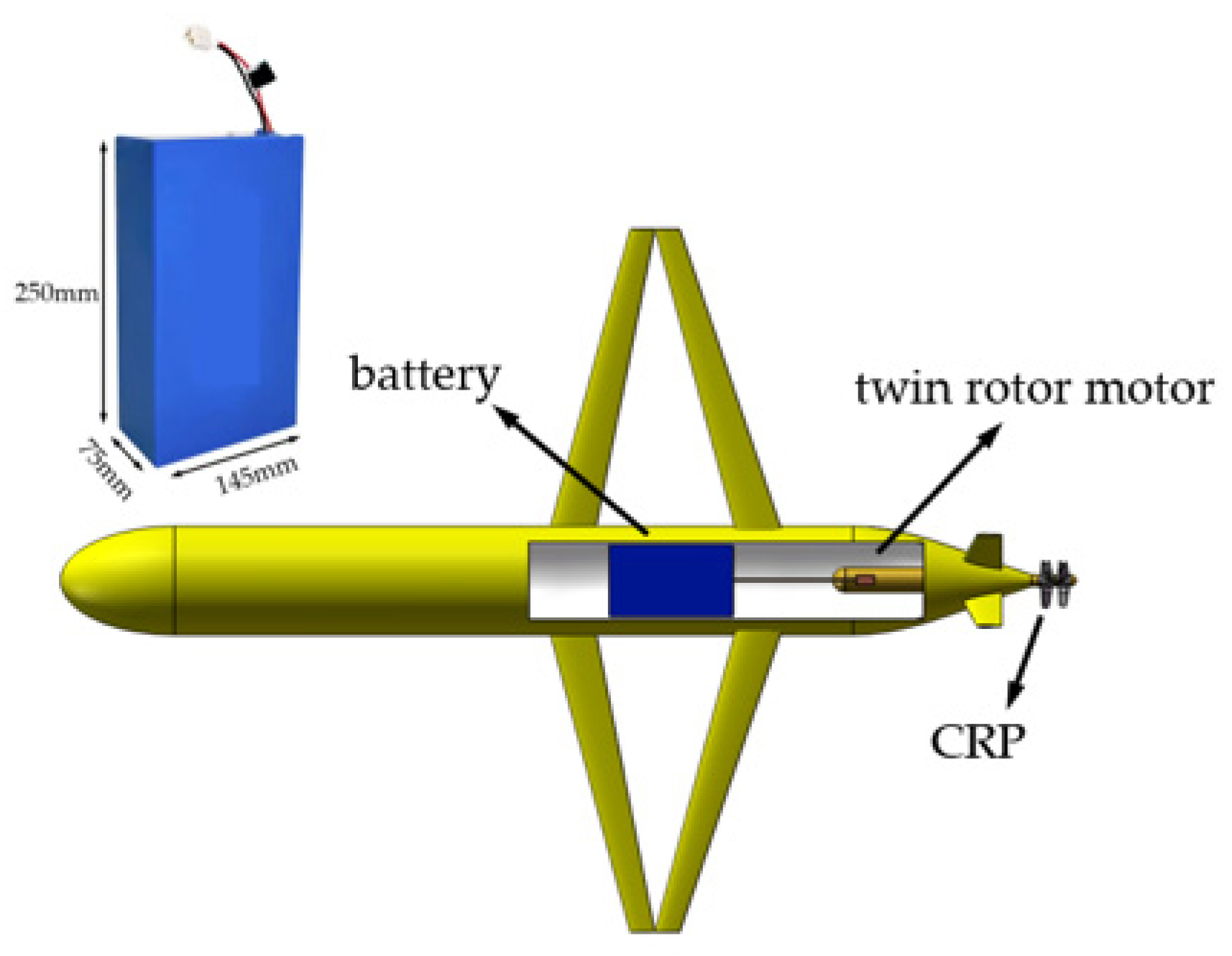
Figure 33.
Concept chart of the battery and the propulsion system.
Figure 33.
Concept chart of the battery and the propulsion system.
Table 1.
Main dimension parameters of the AUG.
Table 1.
Main dimension parameters of the AUG.
| Parameter | Symbol | Value | Unit |
|---|
| Effective maximum length | L | 2.00 | [m] |
| Maximum diameter of the hull | Dh | 0.22 | [m] |
| Length of the bow | L1 | 0.23 | [m] |
| Length of the stern | L2 | 0.40 | [m] |
| Wingspan of the hydrofoil | B | 0.60 | [m] |
| Chord length of the hydrofoil tip | Ct | 0.05 | [m] |
| Chord length of the hydrofoil root | Cr | 0.10 | [m] |
| Wet surface area of the hydrofoil | S | 0.18 | [m2] |
| Displacement volume | ▽ | 0.0646 | [m3] |
Table 2.
The main parameters of the CRP.
Table 2.
The main parameters of the CRP.
| Parameter | Front Propeller | Rear Propeller |
|---|
| Diameter | 112 mm | 108 mm |
| Direction of rotation | Dextral rotation | Levo rotation |
| Number of blades | 3 | 3 |
Table 3.
Calculation results of the self-propulsion state for the hybrid-driven AUG with the single propeller.
Table 3.
Calculation results of the self-propulsion state for the hybrid-driven AUG with the single propeller.
| V (m/s) | n (rpm) | FD (N) | T (N) | Q (N-m) |
|---|
| 1.4 | 800 | 11.044 | 10.980 | 0.247 |
Table 4.
Calculation results of the self-propulsion state of the maneuverable AUG with the CRP.
Table 4.
Calculation results of the self-propulsion state of the maneuverable AUG with the CRP.
| V (m/s) | n (rpm) | FD (N) | Propeller Thrust (N) | Propeller Torque (N-m) |
|---|
| Tf | Ta | T | Qf | Qa | Q |
|---|
| 1.4 | 780 | 10.73 | 6.11 | 4.57 | 10.68 | 0.129 | −0.110 | 0.019 |
Table 5.
The calculation results of the self-propulsion factor of the different hull line AUGs with the CRP.
Table 5.
The calculation results of the self-propulsion factor of the different hull line AUGs with the CRP.
| Hull Line | V (m/s) | VA (m/s) | n (rpm) | J | FD (N) | TB (N) | Q0 (N-m) | QB (N-m) | PE (W) | ηR | η0 | ηH | PB (W) |
|---|
| p = 2; θ = 15° | 1.4 | 1.040 | 780 | 0.7143 | 10.73 | 10.68 | 0.205 | 0.239 | 15.022 | 0.860 | 0.48525 | 1.350 | 26.664 |
| p = 2; θ = 25° | 1.4 | 0.995 | 755 | 0.7060 | 10.14 | 10.01 | 0.194 | 0.220 | 14.196 | 0.882 | 0.48509 | 1.425 | 23.284 |
| p = 3; θ = 25° | 1.4 | 0.999 | 760 | 0.7040 | 10.20 | 10.00 | 0.198 | 0.215 | 14.280 | 0.921 | 0.48505 | 1.429 | 22.369 |


