

Fuel Consumption Prediction Models Based on Machine Learning and Mathematical Methods
by
 ,
,
Xianwei Xie
1,
Baozhi Sun
1,*,
Xiaohe Li
2,3,
Tobias Olsson
4,
Neda Maleki
4 and
Fredrik Ahlgren
4 1
College of Power and Energy Engineering, Harbin Engineering University, Harbin 150001, China
2
China Ship Scientific Research Center, Wuxi 214082, China
3
Taihu Laboratory of Deepsea Technological Science, Wuxi 214082, China
4
Department of Computer Science and Media Technology, Linnaeus University, 39354 Kalmar, Sweden
*
Author to whom correspondence should be addressed.
J. Mar. Sci. Eng. 2023, 11(4), 738; https://doi.org/10.3390/jmse11040738
Submission received: 13 February 2023
/
Revised: 15 March 2023
/
Accepted: 28 March 2023
/
Published: 29 March 2023
(This article belongs to the Special Issue Machine Learning and Modeling for Ship Design)
Abstract
:An accurate fuel consumption prediction model is the basis for ship navigation status analysis, energy conservation, and emission reduction. In this study, we develop a black-box model based on machine learning and a white-box model based on mathematical methods to predict ship fuel consumption rates. We also apply the Kwon formula as a data preprocessing cleaning method for the black-box model that can eliminate the data generated during the acceleration and deceleration process. The ship model test data and the regression methods are employed to evaluate the accuracy of the models. Furthermore, we use the predicted correlation between fuel consumption rates and speed under simulated conditions for model performance validation. We also discuss applying the data-cleaning method in the preprocessing of the black-box model. The results demonstrate that this method is feasible and can support the performance of the fuel consumption model in a broad and dense distribution of noise data in data collected from real ships. We improved the error to 4% of the white-box model and the to 0.9977 and 0.9922 of the XGBoost and RF models, respectively. After applying the Kwon cleaning method, the value of also can reach 0.9954, which can provide decision support for the operation of shipping companies.
1. Introduction
The international shipping community is paying more attention to the issue of greenhouse gas (GHG) emissions with the gradual warming of the global climate. According to the Fourth International Maritime Organization (IMO) GHG Study, the carbon intensity (i.e., CO2 emissions per unit of Gross Domestic Product) of international shipping decreased by 10.7% between 2012 and 2018, while annual GHG emissions rose by 9.6% [1]. In general, the international shipping industry accounts for approximately 2% of global anthropogenic GHG emissions [2]. Meanwhile, shipping companies are more concerned about the energy efficiency of their ships due to the increasing proportion of fuel costs relative to operating costs [3,4]. Energy efficiency improvement and fuel consumption reduction are essential to decrease operating costs and enhance maritime operations’ sustainability [5].
As the ships have gradually become a colossal sensor hub, a massive volume of data is generated [6]. These data sources can lead us to find a method of energy usage optimization using analyzing and monitoring. Mathematical or machine learning methods have been used broadly across industries concerned with data-intensive applications [7]. The mathematical and machine learning models are applied for shipping companies to analyze the data as an energy optimization and decision support system [8,9]. The model reflects the correlation between ship fuel consumption and other parameters, such as speed, main engine power, weather information, etc. [10]. Therefore, we can employ the fuel consumption models as a robust tool to predict and study the fuel consumption law under different sailing states of ships [11]. The models need to be accurate on the validation and test sets with the capability of reflecting the results in the actual situations. In this respect, we are committed to building the models and improving the prediction accuracy under specific requirements.
The rest of the paper is organized as follows. Section 2 reviews existing research on ship energy consumption prediction using mathematical and machine learning models. Section 3 describes the data and the steps of data preprocessing. In Section 4, we build a white- and black-box model and propose a data-cleaning method for the black-box model that improves the performance in a specific scenario. We evaluate the models’ accuracy and interpret the prediction results in simulated conditions drawn in Section 5. Section 6 discusses the effects of these models and the data-cleaning method, which is followed by the conclusions in Section 7.
2. Related Work
There are research foundations regarding ship fuel consumption models. The prediction model is the basis of various optimization and analysis, mainly including mechanism-based analysis and machine learning methods.
The propulsion principles and mathematical analysis of fuel consumption form the basis of the white-box model [12], which includes ship statics and dynamics [13,14]. Ref. [15] modeled the fuel consumption mechanism based on the principle of the ship engine propeller and the law of resistance transfer. Ref. [16] optimized the navigation process using mathematical modeling of ship energy consumption, such as the resistance in different wind and wave conditions. The white-box models are connected internally; therefore, the internal parameters are easily affected by the environment, which incurs errors in the entire model [11]. In addition, the internal parameters cannot be adjusted during the voyage, and the limitation of the resistance calculating formula causes the over-time changes in the propulsion system’s operating parameters to be ignored [8]. Ref. [17] presents a six-degree-of-freedom (6DOF) ship performance model to evaluate the best method of using a pair of Flettner rotors and analyzes the performance of this propulsion system in consideration of weather and sea conditions, evaluating the related reduction in fuel consumption.
While the white-box model represents the relationship hidden in the formula, the black-box model finds a relationship based on data, which helps to explain information and make decisions [18]. Therefore, it is necessary to analyze the data generated by ships in different states through classification and clustering methods. Statistical analysis is one of the ordinary and widely accepted methods of the black-box model and can be explained in some way [15]. Ref. [19] analyzed different trim values of engine fuel consumption rates and achieved optimal sailing conditions by identifying different draft values. The authors proposed a data processing framework, including preprocessing, post-processing, a data-driven model, sensors, and fault identification [20].
However, the authors of [11] state that the machine learning models sacrifice interpretability but enhance predictive accuracy compared to statistical analysis [11]. Ref. [21] calibrated fuel consumption–speed curves by polynomial regression based on 418-noon report data, thus obtaining a set of ship fuel consumption–speed curves that can be used under most weather conditions and loading conditions. Ref. [22] proposed the fine segmentation of the shipping route using the Hadoop and MapReduce frameworks [23] by applying the ship’s sensor data. They optimized the engine speed of inland ships by finding the optimal segment set using the particle swarm optimization algorithm. Ref. [24] produced an artificial neural network (ANN) model using the noon report data. Then, they optimized the speed and trim by a two-stage, shore-based, and offshore optimization method during navigation. Because of the nonlinearity of the ANN model, the authors proposed a dynamic programming algorithm to solve the objective function of the optimization problem. Optimizing speed and trim can reduce ships’ fuel consumption by 2–7% in actual navigation. Ref. [25] proposed a random forest model for the prediction of the fuel consumption of dry bulk carriers based on 242 noon-report data. The mean absolute percentage error (MAPE) reached 7.91% in the model’s evaluation results. Moreover, it can save 6.53% of fuel consumption after speed optimization. However, there is an inherent uncertainty in this noon-report data [26], which can be solved by the onboard continuous monitoring system data. Ref. [27] studied the performance of three models based on data: black-box, white-box, and gray-box models. The authors of this reference proposed a new strategy for optimizing the trim of a vessel, and the results showed that the BBM can remarkably improve on the state-of-the-art WBM. At the same time, the GBM can encapsulate the a prioro knowledge of the WBM into the BBM.
The black-box models can capture the impact of weather/sea conditions and other external factors on ship fuel consumption from continuous sensor data [28,29,30]. The accuracy and simplicity of the black-box model can also provide an illustration and potential for ship energy consumption analysis [31,32]. The importance of data preprocessing has increased due to the black-box models’ dependence on data, which can reflect the relationship between the various parameters of the ship. Ref. [33] removed the NaN and zero and measurement errors for speed and fuel consumption values in sensor data. Ref. [34] identified and rejected the engine transients and recording anomalies and extracted valuable features and standardization. Ref. [35] detected and synchronized data discontinuities in time. They also removed the ship’s maneuvering (dynamic) conditions in the sea passage, such as voluntary acceleration and deceleration, sharp power increases, and sharp course changes. Ref. [36] proposed a data-driven solution based on deep learning sequence methods and historical ship trip data to predict ship speeds at different stages of a voyage. The results showed that deep learning models combined with maritime data can leverage the challenge of estimating ship speed and improve shipping operational efficiency, navigation safety and security, and ship emissions estimation and monitoring. Ref. [37] developed the application of artificial neural networks (ANN) to predict the total fuel consumption of ships in various operational scenarios and applied state-of-the-art deep learning techniques for training and optimizing feedforward neural networks (FNN). The performance of the ship’s propulsion model can be improved, leading to an improved understanding of the ship’s performance regulation and reduction of fuel consumption and emissions. Ref. [38] introduced an innovative platform that coordinates data collected from various sensors on board through Big Data technology and implements extreme-scale processing techniques to perform operational efficiency and performance optimization. The technology of data collection and processing has been gradually improved.
Through the above literature analysis, we consider an oil tanker’s continuous dataset, including ship parameters and ship model test data, as the research direction. This paper establishes two black-box models and a white-box model. We propose a data cleaning method using Kwon’s formula as the primary calculation method. We discuss the results in the prediction accuracy of different models for a future research line.
3. Data Description and Preprocessing
The raw sensor dataset in this study is the sailing test case from an oil tanker that contains 496 data features (operating parameters). While we participated in the trial, due to the defeat of sensors, there were fault signals in the collected data. The remaining 378,468 (4.38 days) data records were retained, and the data collection time unit is seconds. The raw data usually have noise that can cause over-fitting or mislead the decision of the model [39], which results in a lower generalization ability of the model. Data preprocessing always has an essential effect on the generalization performance of a supervised machine learning algorithm [40].
In this study, most features are alarm signal detection points and various temperature, pressure, flow, and other detection signals. Optimizing fuel consumption is paramount to shipping companies as it directly reflects the navigation economy, surpassing rpm and power. To this end, FCR has been chosen as the model output. We need to filter the data and select the modeling features relevant to the ship’s fuel consumption, such as speed, engine power, trim, and draft. Furthermore, the model needs to consider the influence of selected parameters on fuel consumption. The correlation between engine power and fuel consumption will cover the impact of ship speed and other features. The interior features selected for modeling are speed, fuel consumption rate (FCR), trim, and fore and aft draft. Furthermore, external features such as wind and waves also impact ships’ fuel consumption. Due to the lack of wave and current features in the sensor dataset, we parsed the wave data (wave height and wave direction) from ECMWF (European Centre for Medium-Range Weather Forecasts), matched into the sensor data according to the geographical location (latitude and longitude) and collection time. Considering the relative relationship between absolute wind direction and ship heading, we calculated the angle between the absolute wind direction and the heading as the relative wind direction. Considering the symmetry of the ship, the wind from the port side and the starboard side has the same impact, so the relative wind direction ∼ is converted to ∼; means the wind is from the bow and is from the stern.
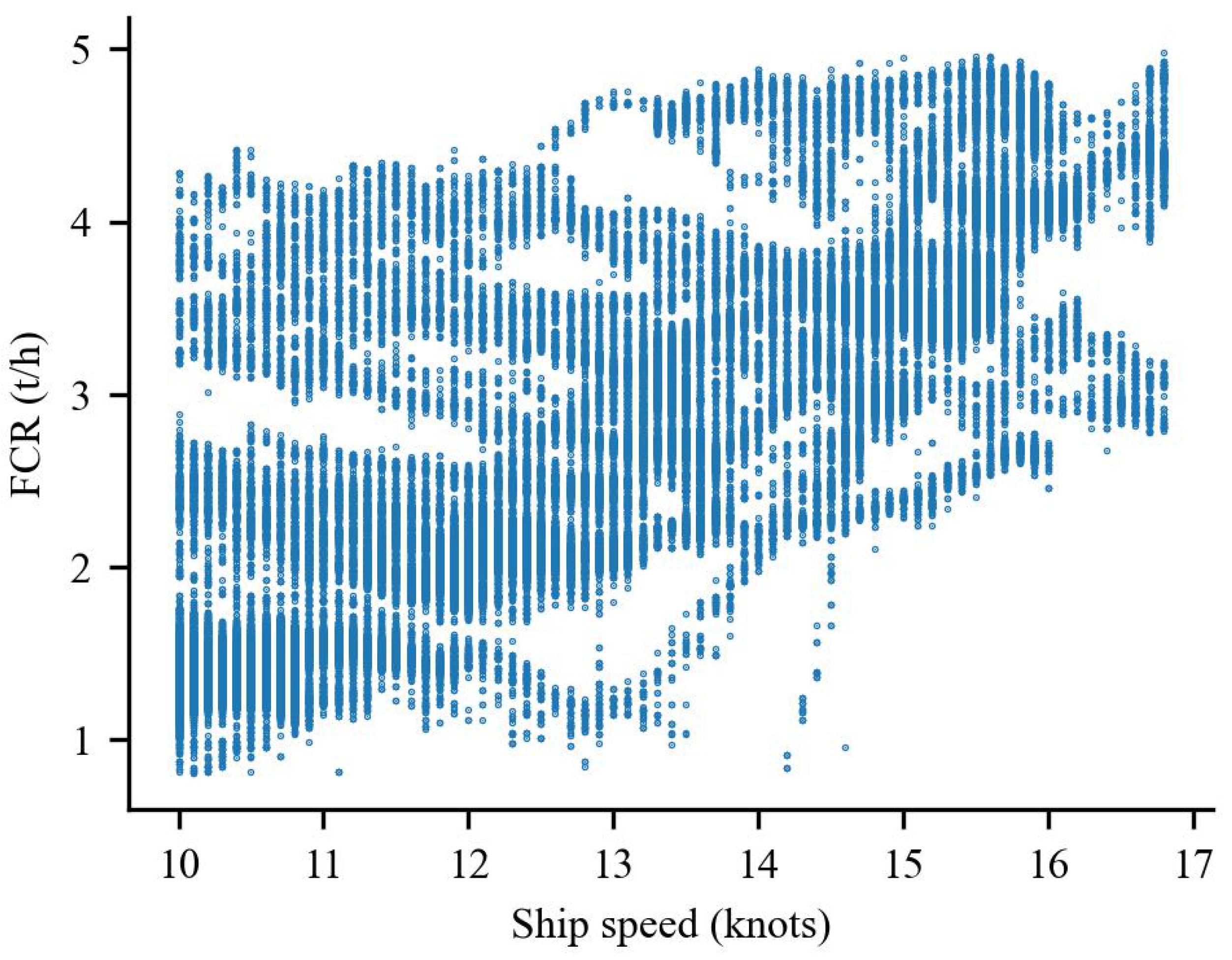
After extracting the above data features from the sensor dataset, the following data preprocessing was carried out. First, we removed the data of FCR, wind speed, and wind direction values lower than 0. Second, we removed the speed data out of the range of 10 to 16.8 knots (determined by the ship design speed and the maximum speed under full load). After excluding the data below 10 knots, there is no berthing and start-up acceleration). The dataset includes nine features: ship speed (V), fore draft (D), aft draft (D), trim (T), wave height (Wave), wave direction (Wave), absolute wind speed (Wind), wind direction (Wind), and FCR, resulting in 147,845 rows after these steps. Figure 1 shows the data distribution of ship speed and fuel consumption. The statistics of the data are shown in Table 1. Figure 1 is the speed and fuel consumption distribution; the fuel consumption values cover the range of 1 to 4 tons/h in the speed range below 14 knots. It is not easy to find the cubic relationship among them. During the ship’s sea trial process, the acceleration and deceleration processes result in high fuel consumption at low speeds that do not meet standard navigation. Further data processing is necessary if some optimization analysis is performed based on the model.
4. Fuel Consumption Prediction Models
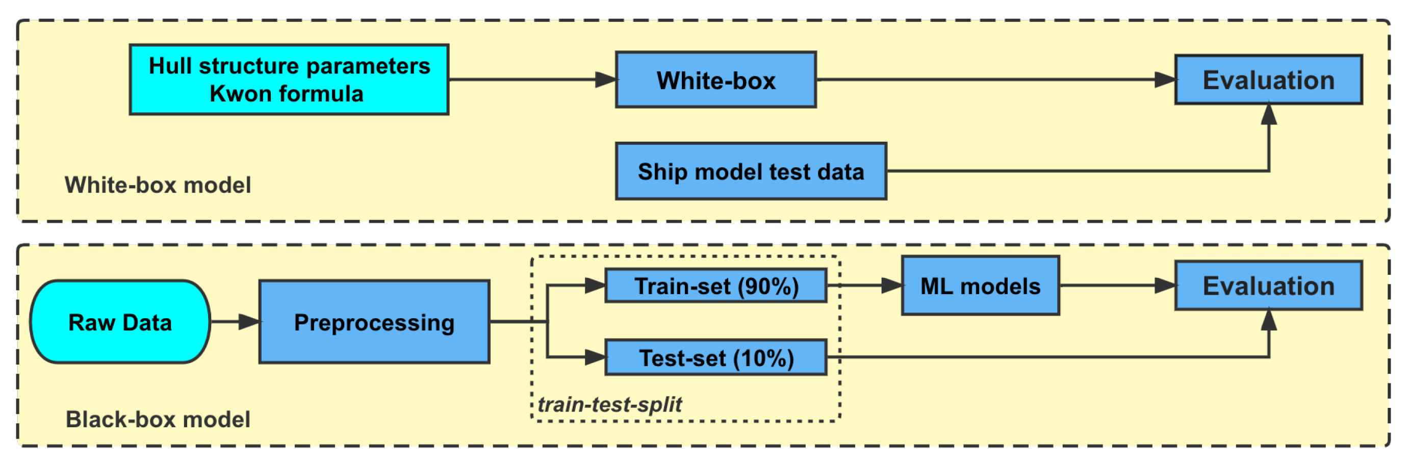
We establish two types of models to predict the FCR: white-box and black-box (ML, machine learning) models. Figure 2 is the flow chart of the model building. In the following, we will explain the models and method in detail.
4.1. White-Box Model
The white-box model in this paper is based on this ship’s structural and main-engine parameters and adopts the same method as Li [16]. We carried out the calculations through mathematical formulas and the principle of energy transfer. As shown in Figure 2: White-box model, we used hull structure parameters and the Kwon formula to build the white-box model and used ship model test data to evaluate the model.
Ships will increase additional resistance to the wind and waves, which is reflected in the loss of speed. Li calculated the fuel consumption of the main engine from two parts: the consumption of sailing in still water and the additional consumption to keep the speed constant under irregular wind and waves. Still water is used in the model test of the ship; the purpose is to calculate the resistance caused by still water to the ship’s navigation, and still water is a situation where there is no wind and waves. In the case of still water, the adequate power of the ship can be obtained by calculating resistance in the water. After that, we can calculate the FCR by fitting the main-engine performance parameter data.
Considering that the highest absolute wind speed in the sensor dataset is 24.4 knots, the corresponding Beaufort wind level (Beaufort number [41], Bn) is 6, so we do not need to consider the impact of voluntary deceleration losses (Bn greater than 7) on Kwon’s formula. It is necessary to provide greater power and thus generate additional fuel consumption to keep the ship at its original speed under the different wind and wave conditions [16]:
where is the additional fuel consumption caused by the unchanged speed of each segment under the influence of irregular wind and waves, ; is the specific fuel oil consumption, ; is the shaft efficiency; is the propulsion efficiency; is the additional power of the main engine, W; and is the additional effective power, W.
The Kwon formula can calculate the specific value of additional effective power according to conventional sea conditions. Kwon proposed corresponding formulas for calculating ship speed loss and additional effective power [42,43]:
where n is an empirical constant related to types of ship and loading status; is the effective power of the ship in calm water; is the speed loss caused by wind and waves, ; is the speed in calm water, ; is the ship’s speed in selected weather (wind and irregular waves), ; is the direction reduction coefficient; is the speed reduction coefficient; is the ship form factor; is the ship length between perpendiculars, m; and g is the local acceleration of gravity, .
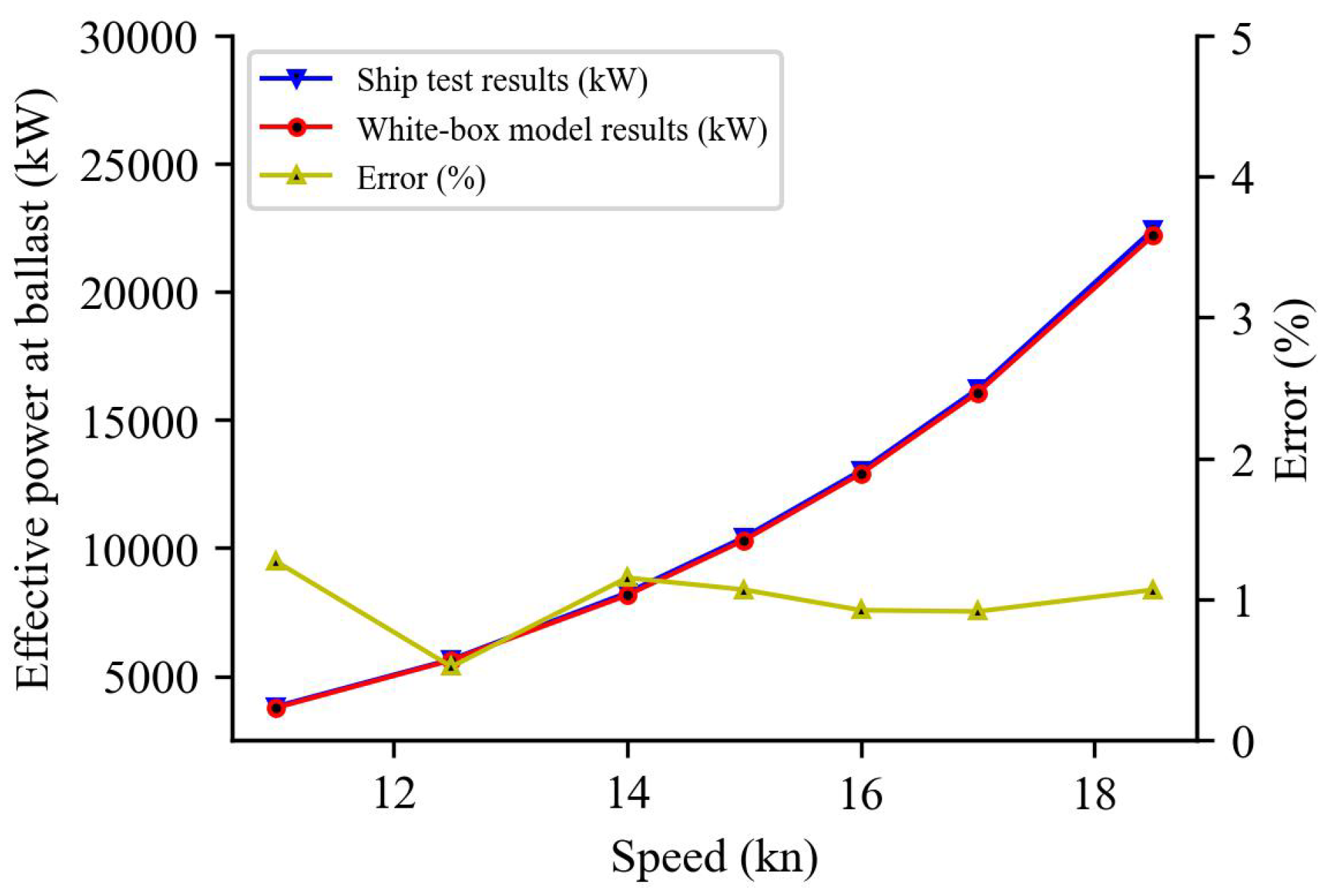
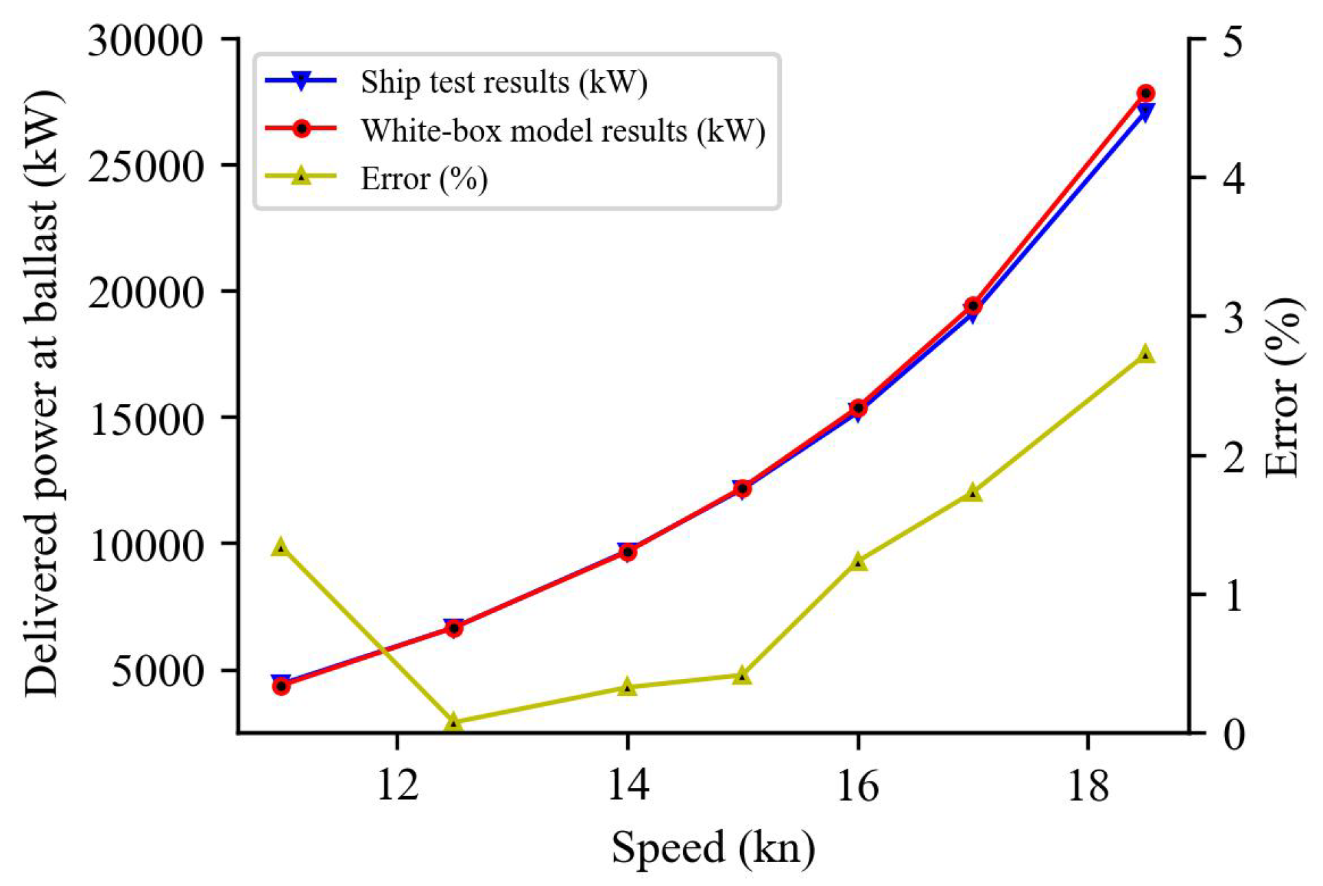
The effective power is the power available at the output side of the engine, i.e., at the crankshaft flange of the engine, which connects it with the flywheel and the rest of the intermediate shaft. The delivered power is the power delivered to the propeller, which includes the losses due to the gearbox, the bearings, and the stern tube seal [44]. The white-box model’s process is the above fuel consumption calculation and the still water situation. The input parameters of the white-box model are speed, loading type (full or ballast), Beaufort wind rate, and wind direction. According to the output power, we can calculate the fuel consumption.
4.2. Black-Box Model
To compare the efficiency and performance, we built two black-box models based on the dataset after preprocessing: random forest (RF) and Xgboost. RF and XGBoost have the following advantages (take the ANN algorithm as an example):
- (1)
- Strong interpretability: The tree-based algorithms can provide each feature’s importance and have strong interpretability. In comparison, ANN is brutal in explaining the contribution of each feature.
- (2)
- Fast training speed: RF and XGBoost can be processed in parallel, and the training speed is fast. In contrast, ANN requires iterative optimization of the backpropagation algorithm, and the training speed is relatively slow.
- (3)
- Strong robustness: RF and XGBoost are relatively robust to outliers and noise and are not easily affected by extreme values. In contrast, ANN is sensitive to outliers and noise and requires data preprocessing.
- (4)
- Can handle high-dimensional data: Random Forest and XGBoost can handle high-dimensional data very well, and the problem of dimensionality disaster is challenging. In contrast, ANN requires dimensionality reduction when dealing with high-dimensional data.
After the preprocessing, we divided the data into training and test sets by the ratio of 9:1 [45] according to the random partition method, shown in Figure 2: Black-box model. We used the training set to build and validate the model and used the test set for final evaluation. The connection between FCR and the environmental factors displayed a significant non-linear pattern, and the dataset size made it challenging to predict FCR accurately. Therefore, the forecast model for marine environmental factors should incorporate XGBoost regression and RF strategies to improve its overall performance [46,47].
4.2.1. RF Model
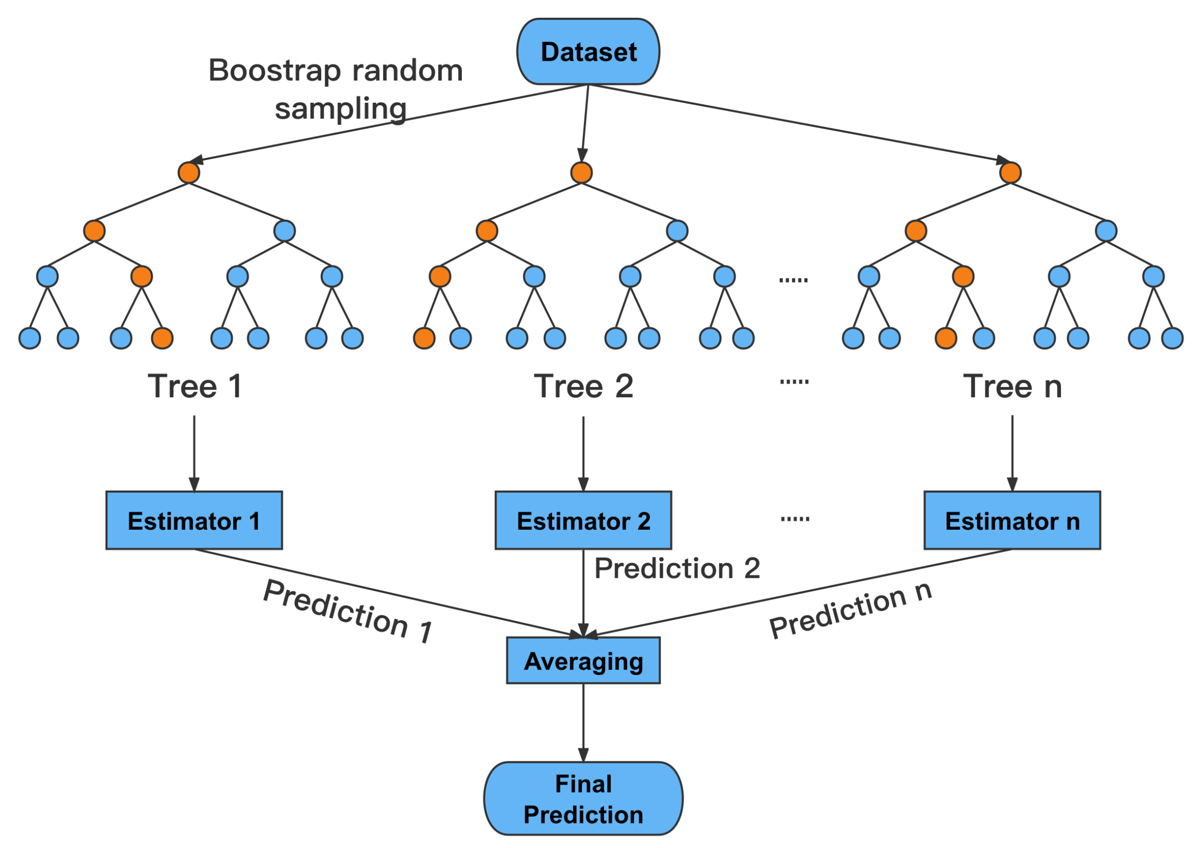
RF is a bagging ensemble learning algorithm that integrates multiple decision trees. It was first proposed and developed by [48]. RF uses the decision tree algorithm to construct each estimator in bagging and then takes the average prediction result of all estimators. The schematic diagram is shown in Figure 3. RF conducts a random sampling of sample data and features to construct diversified decision trees, so it can reduce the variance of the model to some extent and effectively alleviate the overfitting phenomenon.
4.2.2. Xgboost Model
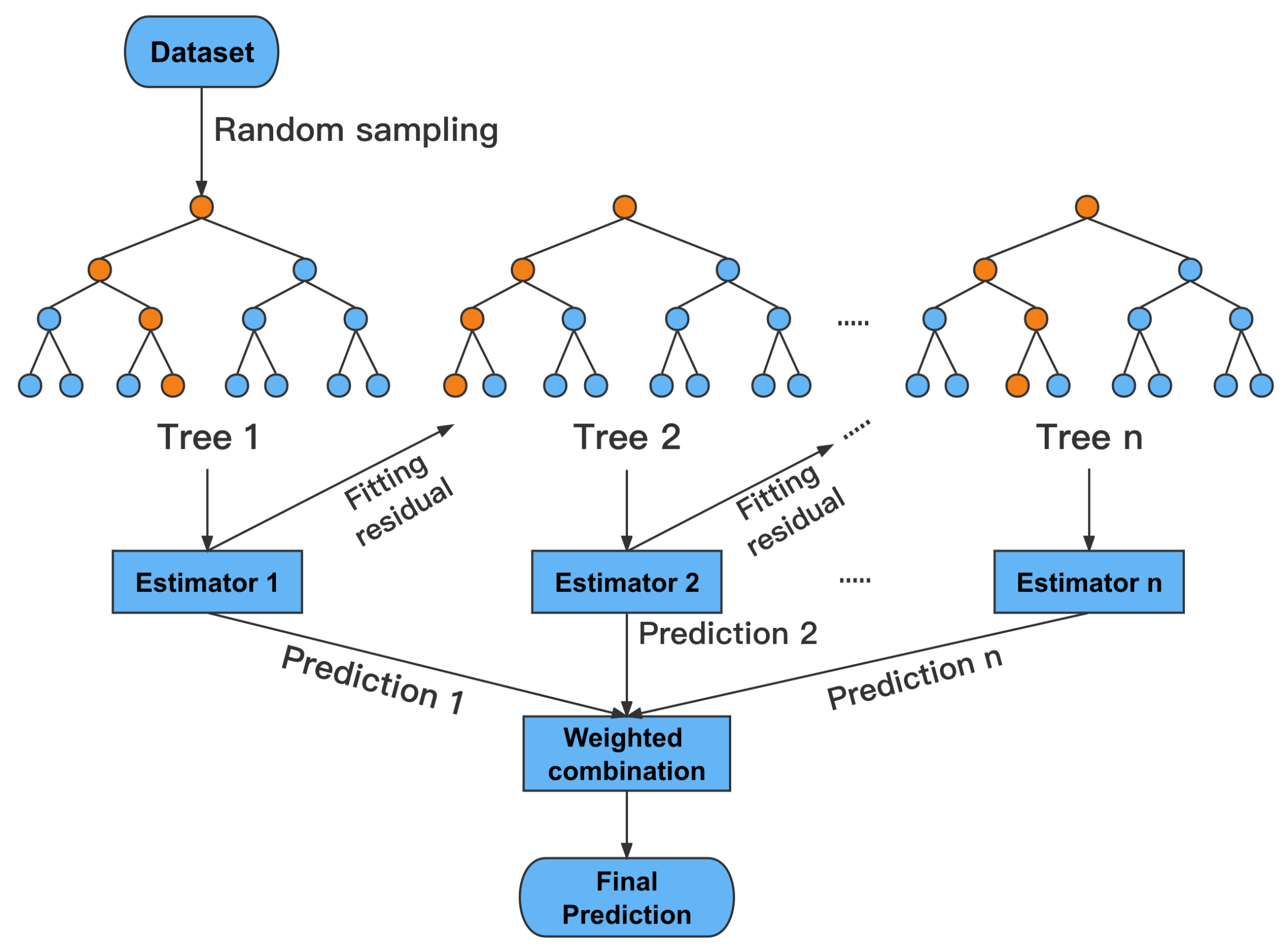
Xgboost is a distributed gradient boosting algorithm based on the gradient boosting framework, which aims to build boosting trees in order, efficiently, flexibly, and conveniently to solve the regression problem. Xgboost is essentially an improved version of the gradient boosting decision tree (GBDT), initially developed by [49]. Xgboost solves the problem that GBDT cannot be calculated in parallel and is easy to overfit [50], so it has a higher fitting performance. The schematic diagram of Xgboost is shown in Figure 4.
4.2.3. Hyperparameter Optimization (HPO)
The establishment process of the HPO teammate model is critical, as it directly determines the accuracy of the model [51]. To obtain the best model hyperparameters, we used the grid search method to perform 5-fold cross-validation (5-fold cross-validation: we divided the dataset into five parts, using four parts for model training each time and the remaining part as the validation set, resulting in five times of training and validation; the average results are the final validation result). We optimized the hyperparameters, ‘’ and ‘’, together. Each decision tree was trained by randomly sampling the training dataset and selecting a subset of features. Therefore, the number of trees (‘’) is a crucial hyperparameter affecting the performance of random forest models. ‘’ refers to the maximum depth of the decision tree, that is, the maximum distance from the root node to the leaf node, and branches exceeding this depth will be pruned. ‘’ is one of the most commonly used hyperparameters in decision tree models, which controls decision tree complexity and generalization ability [52]. The optimization range of the two parameters we specified is as follows: ‘’ ranges from 100 to 3000, and every 200 is one step-size, resulting in a total of 15 parameter values; ‘’ ranges from 3 to 15, and each value is one step-size, resulting in a total of 12 parameter values. From this, HPO requires fitting five folds for each of the 180 candidates, totaling 900 fits. Regarding accuracy, we use to validate the model.
4.3. Black-Box Model Cleaning Method
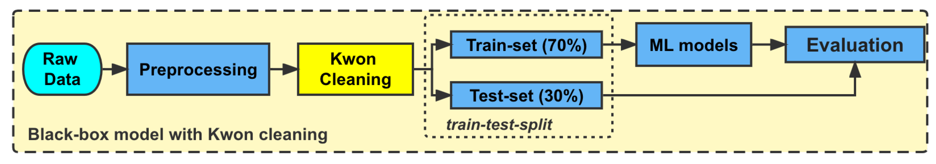
The ship will face various conditions during the operation. For such a distribution (Figure 1), the machine learning models cannot use prior knowledge to judge the data quality but can only use the data for modeling. A novel approach to data cleaning is introduced in this study, which involves the use of Kwon’s formula as the primary calculation method. It can effectively solve this problem. We calculate the percentage range of fuel consumption generated by wind and waves during steady-state navigation. As shown in Figure 5, we apply Kwon’s formula as prior knowledge to perform a cleaning method on the sensor dataset after the first preprocessing step and divide the training and test sets to build and evaluate the model. Because of the varying data size, we have opted for a training–test split ratio of 7:3.
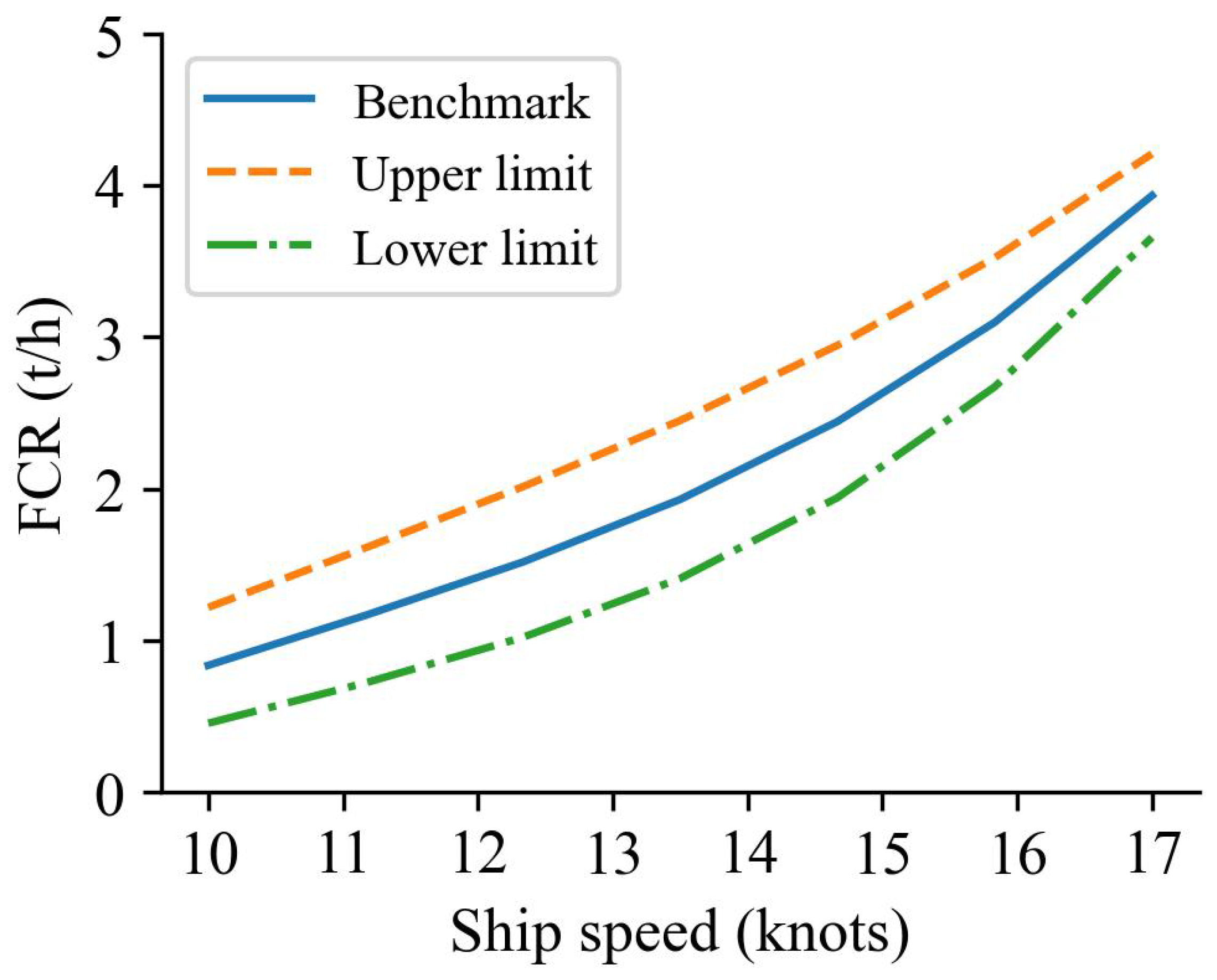
This Kwon cleaning method contains two steps. First, we used the polynomial fitting method to obtain the standard speed–fuel consumption curve under still water conditions based on the ship test data. The standard speed–fuel consumption curve is used to calculate the fuel consumption at each speed, which is then used as the fuel consumption benchmark. Second, the additional fuel consumption percentage of the ship was calculated by combining Kwon’s method with the maximum wind level (Beaufort wind level 6) and using the headwind as the calculation criteria for the upper and lower limits of fuel consumption to eliminate the over-limit data.
5. Results
After building the black- and white-box models using ship operation sensor data and ship parameters, we optimized the hyperparameters using the five-fold cross-validation grid search method. We used the evaluation and prediction results to verify the model’s prediction performance.
5.1. HPO Results
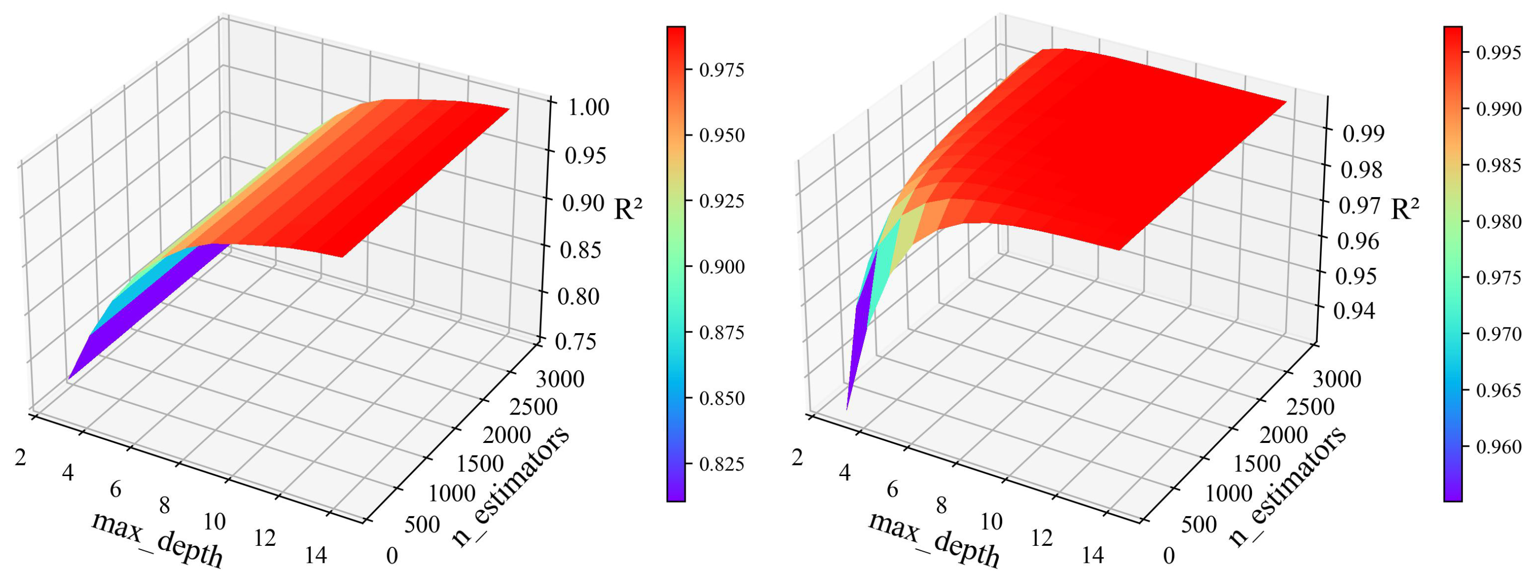
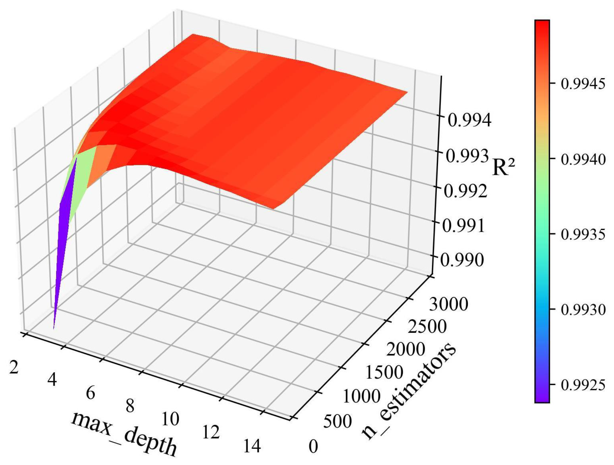
After the HPO, we drew a 3D graph of the validation results as a function of the two parameters, as shown in the Figure 6. From the range of ‘’ and ‘’, HPO requires fitting five folds for each of the 180 candidates, totaling 900 fits. Regarding accuracy, we used to validate the model. After optimization, we draw the 3D graph of the validation results as a function of the two parameters (RF and XGBoost), as shown in Figure 6. In this paper, we used the Jupyter notebook IDE with Python 3.9 version for the implementation and visualization; we did not use frameworks or libraries such as PyTorch and TensorFlow. We show the results of the model’s execution time in Table 2.
In terms of running efficiency, the RF model takes 32,955.05 s in 900 fits, which is 9.15 h. Compared with the RF model, the XGBoost model took 54,139.69 s under the same conditions, which is 15.04 h. Since the dataset used for training was large, and the optimization time increases with the optimization parameters, the optimization would last several hours. Secondly, since the RF model is calculated in parallel, it will take a relatively short time, but XGBoost will not.
From Figure 6, we can see that the difference between the RF and XGBoost model is the sensitivity of the ‘’ parameter to the in the HPO process. The does not change much when the ‘’ increases in the RF model, and the XGBoost model has a response to an increase in both parameters, which will jointly affect the model’s accuracy. After optimization, the result given by RF is that ‘’ is 14 and ‘’ is 900. In XGBoost, ‘’ is 9, and ‘’ is 2700. The two models’ verification results in are 0.9921 and 0.9973, respectively. We can also see from Figure 6 that even with the worst parameter selection, the accuracy of XGBoost is comparable to the highest accuracy of RF, and reached 0.94 (relative to the overall accuracy). Due to its excellent parallel computing capability, the RF model will save time in HPO. The accuracy of the XGBoost model will be relatively higher, and the accuracy of these two models is sufficient.
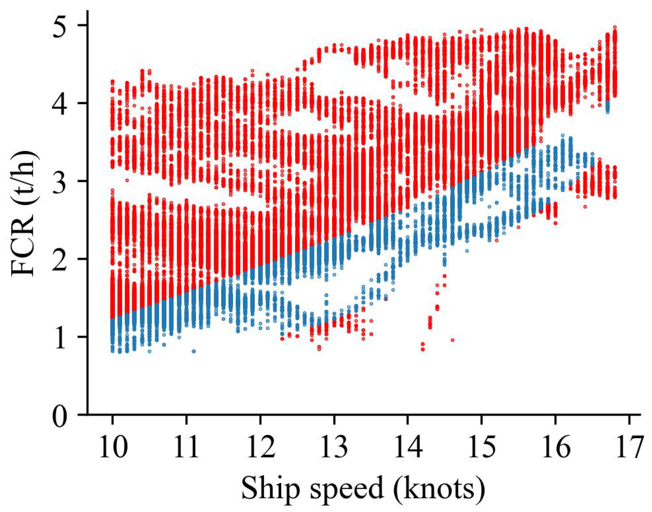
After using the Kwon cleaning method, we calculated the fuel consumption benchmark and its upper and lower limits, shown in Figure 7. The data distribution of speed–fuel consumption after removing “abnormal” data (the unsteady navigation data defined by the Kwon formula are mainly the acceleration and deceleration process) is the blue area shown in Figure 8, and the red zone is the removed “abnormal” data. After firing, the distribution of speed–fuel consumption data is more in line with the ship’s situation during normal navigation. After cleaning by Kwon’s formula, the dataset contains 29,133 data records for nine features.
We used the XGBoost (RF is also available) to model the processed data by the same method for HPO, where ‘’ is 9, ‘’ is 100, and is 0.9950. After reducing a large amount of data, the HPO takes 5221.04 s, which is 1.45 h. Figure 9 shows the variation of with two parameters. After reducing the amount of data, began to partially decline after increasing to a specific value, indicating that after a certain accuracy, the result of the joint influence of ‘’ and ‘’ will appear. However, the influence of a single parameter remained stable, which may be due to overfitting. We conducted further verification based on the model evaluation results.
5.2. Model Evaluation Results
Ship model test data are the most comprehensive assessment of a new boat’s power requirements and can be obtained by experimenting with a model hull and propeller in a towing tank [53,54]. We used the ship model test data of this ship as the validation dataset for the white-box model. The yellow lines in Figure 10, Figure 11, Figure 12 and Figure 13 show the relative error percentage (error), which is less than 4% in all the cases of full load and ballast. This experiment demonstrates that the white-box model’s prediction under still water can adequately reflect the influence of ship resistance on power and fuel consumption.
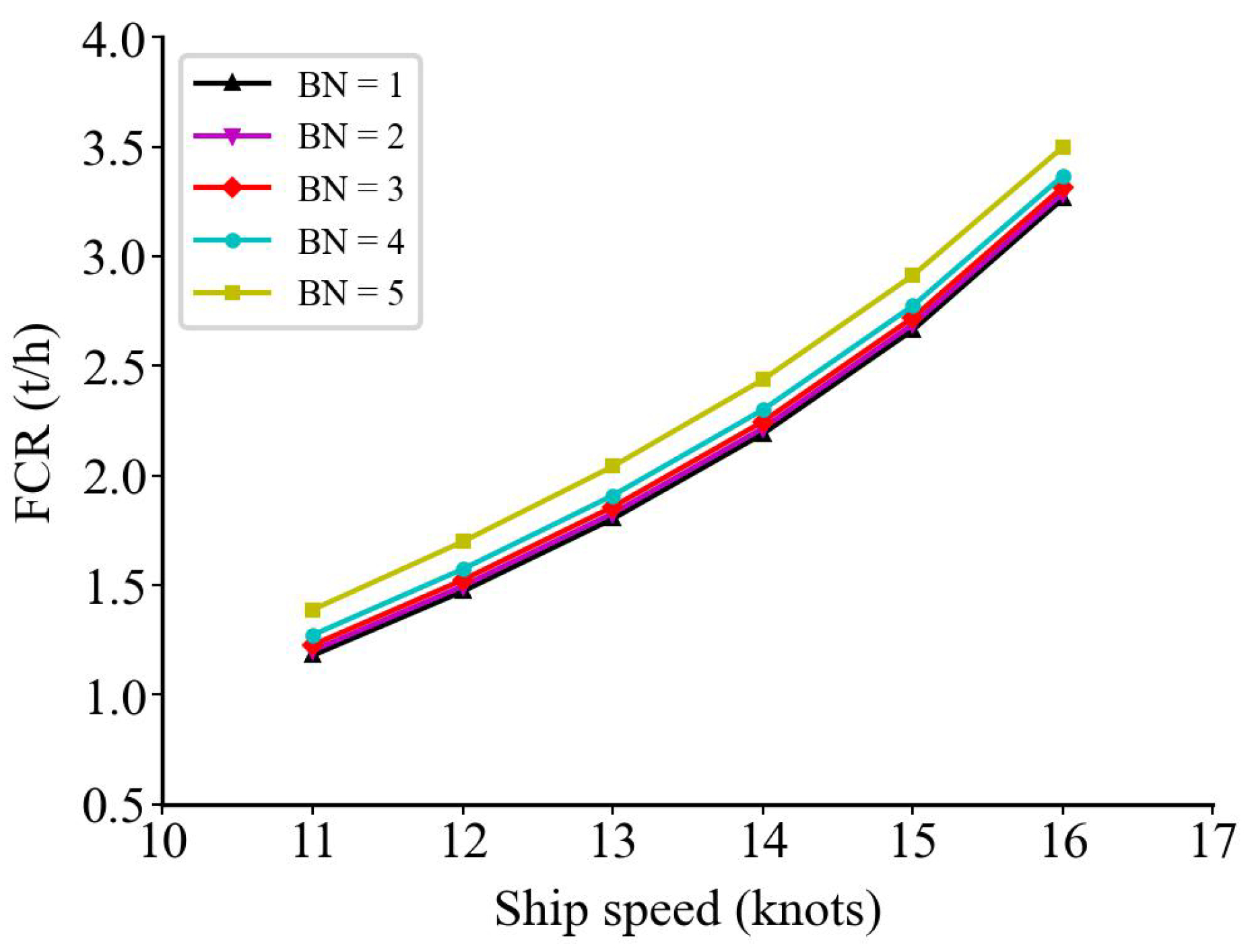
As shown in Figure 14, we simulated the gradually increasing BN scale under headwind conditions, i.e., the wind direction is close to 0 degrees, to verify the additional fuel consumption due to the wind and waves. We notice that the additional fuel consumption grows with the increasing BN scale, which can demonstrate that the calculation of the additional fuel consumption due to the wind and waves using the Kwon formula is feasible [16].
The black-box models, as a type of regression model, can be evaluated using mean square error (MSE), root-mean-square error (RMSE), mean absolute error (MAE), MAPE, and R-squared (). We extracted one-tenth, i.e., 14,785 records of the data, before applying the cleaning method as the test dataset. The evaluation formulas are calculated as follows:
where n is the number of samples; is the true value; is the predicted output value of the model; and is the average value of the samples.
The evaluation of the results was carried out ten times by randomly splitting the training–test dataset (training–test split) and calculating the result each time. Table 3 shows the average results of these ten iterations, followed by the of every time evaluation in Table 4. Both models have accurate evaluation results. The of XGBoost is 0.9977, and that of RF is relatively similar at 0.9922, indicating that the models have extreme performance on the test set. Furthermore, the R2 and the small value of MAE show that the confidence level is high and equals 0.99.
After applying the Kwon cleaning method, we used the same method to re-evaluate the model. Owing to the reduction in the amount of data compared to the raw data, we used 30% of the dataset as the test set, that is, 8740 data points. The average results of the ten times random training–test split are shown in Table 5. The table shows the model’s promising predictive performance.
Thanks to the HPO, the models had high prediction accuracy on the test set, which was similar to the results on the training set. The randomly selected test set implementation did not participate in the model’s training process. Thus, the evaluation results are credible, and it also demonstrates that the model is not over-fitting. To visualize the model’s prediction performance, we randomly selected one hundred values from the model’s predicted result and compared them to the real ones. Figure 15 is the QQ (quantile–quantile) plot of the model prediction and real data. The red line shows the normal probability distribution. The values (blue and green lines) are not entirely overlapped with the red line, which means that the data are not completely normally distributed. Furthermore, the t statistic and p-value are 0.0436 and 0.9652, respectively. These two values show that model prediction and the real data are from the same distribution, which proves the model’s accuracy.
5.3. Model Prediction Results
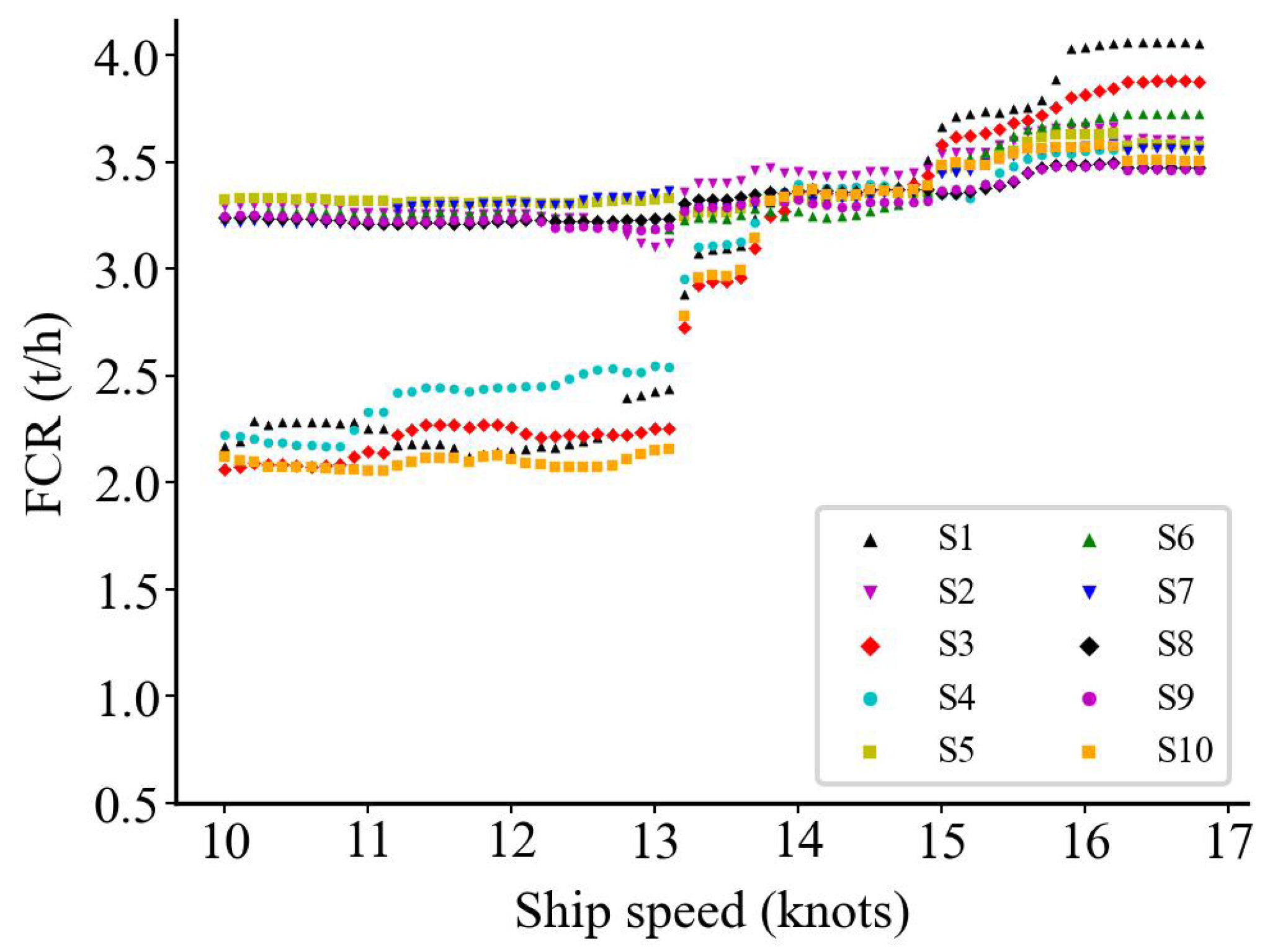
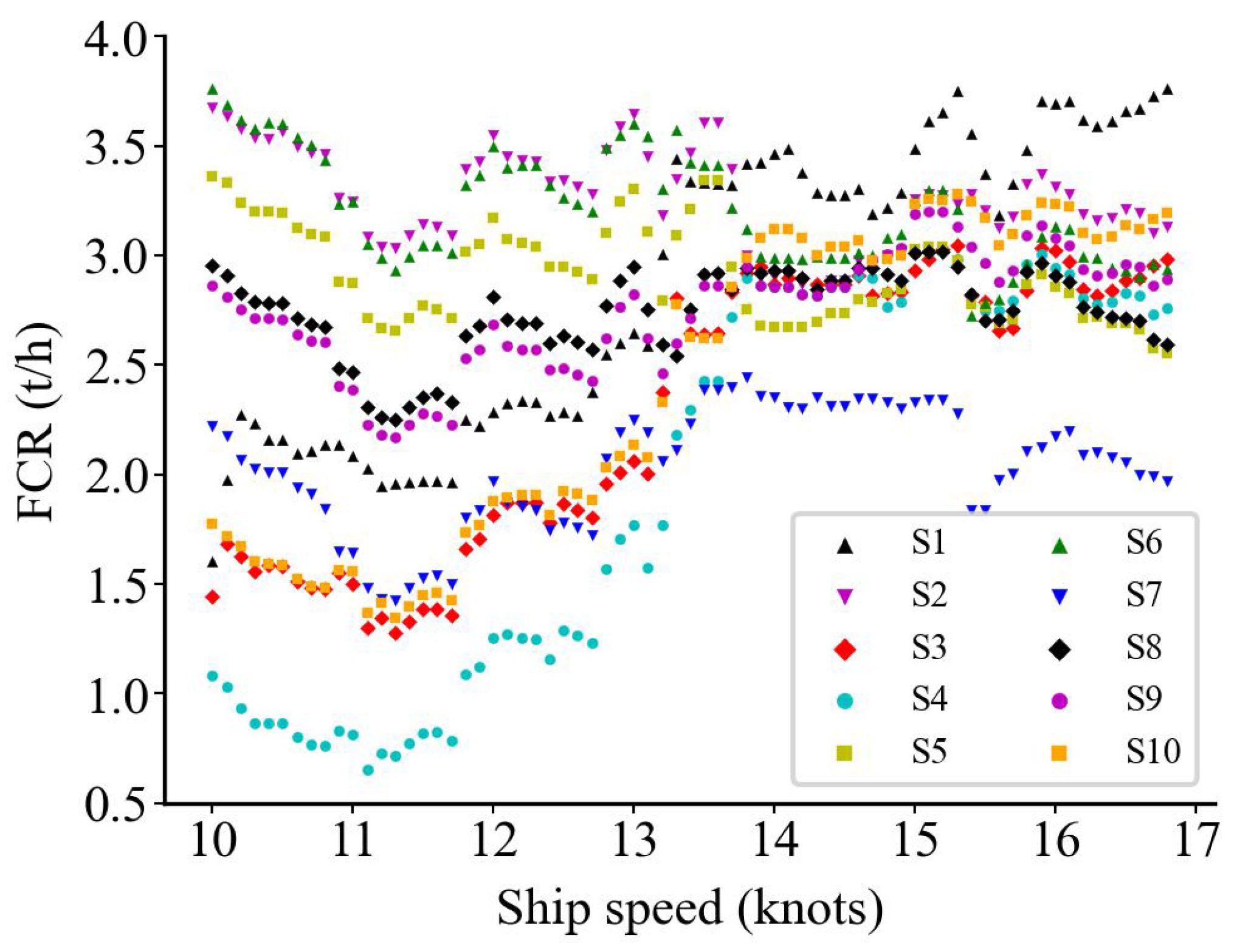
We simulated ten different wind and wave conditions to investigate if the prediction results align with expectations (Table 6). In each condition, the model predicts the condition by changing the speed values discretized by 0.1 knots from 10 to 16.8 knots (a total of 69 values). We obtained the relationship between the predicted FCR and speed, shown in Figure 16, Figure 17 and Figure 18, where S1 to S10 are the ten simulated weather conditions.
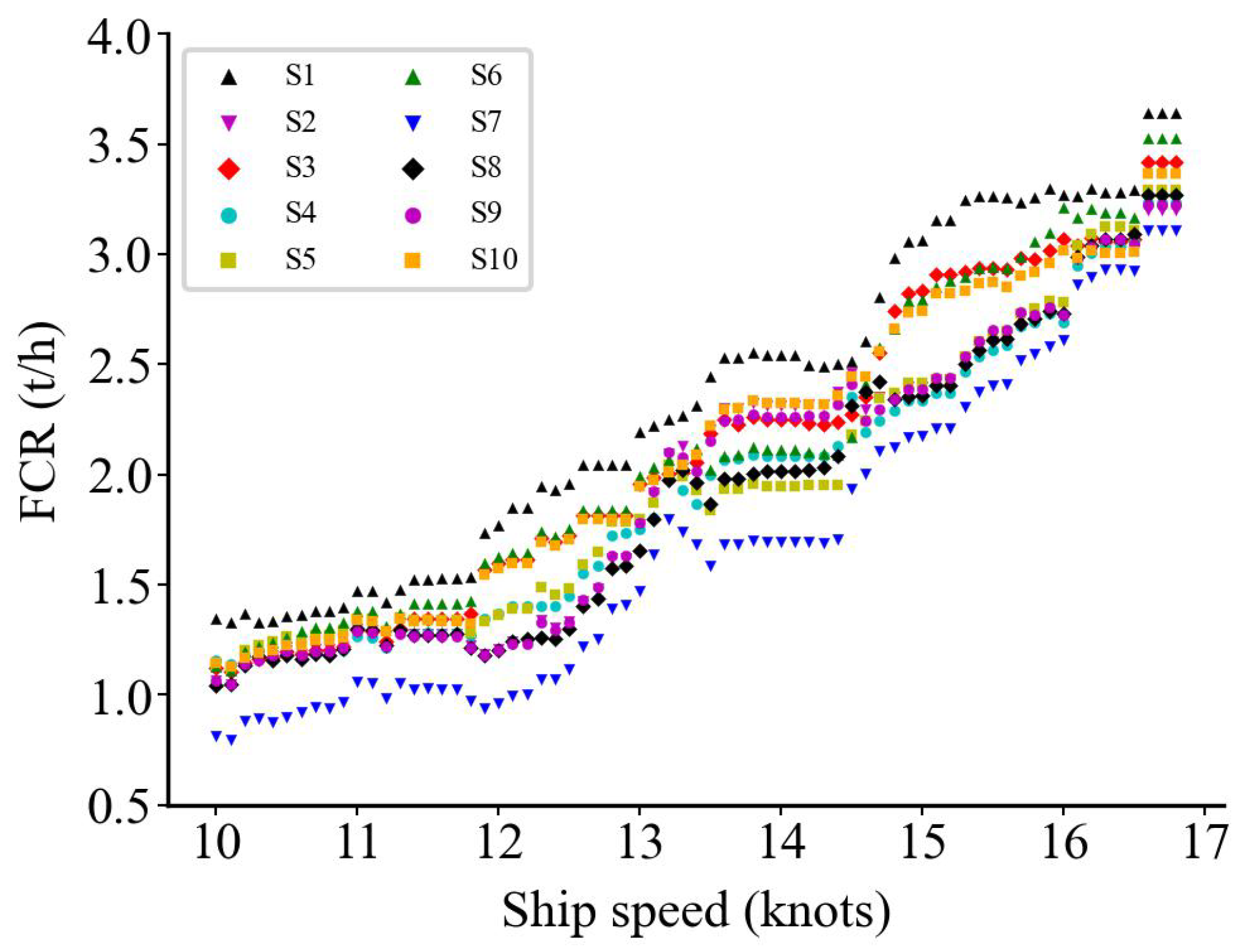
In (Table 5), the simulated features and speed are the input of the models, whereas the models predict 69 times in each condition. Compared to Figure 16, Figure 18 is more practical for predicting the relationship between speed and fuel consumption under real conditions. Figure 18 also shows that the data cleaning method is appropriate for the preprocessing and is effective in modeling.
6. Discussion and Future Work
Based on the assessment outcomes, all the models forecasting the FCR within their respective conditions achieve an acceptable accuracy. Moreover, in the prediction results, the black-box models need to reflect the relationship between speed and fuel consumption regularity. The quality of data collected during the voyage will directly affect the model’s accuracy. The black-box model’s machine learning methods are used for training and predicting data and cannot reflect prior experience in some cases; for example, fuel consumption is cubic related to speed. Then, it is required to have algorithmic accuracy verification and to discuss the cases where we consider prior experience.
During sailing, there is a process of acceleration and deceleration, which are the main reasons that there are higher fuel consumption values under lower speed in the raw data (or lower fuel consumption values under higher speed, as shown in Figure 1). These values are not outliers, though they affect the reliability of ship energy consumption prediction and related optimization research. However, we have filtered the data with speed values lower than 10 knots in the preprocessing; still, accelerations and decelerations above 10 knots remain. This process lasts only a short time compared to regular sailing (ten days more), especially for ocean-going vessels. There are many of these processes because it is a sailing test. The data in this process that may not be used will affect the decision of the models. As a cleaning method, calculating additional fuel consumption for a ship in wind and waves can significantly solve the problem. Above all, having accuracy with no reflection on the real situation is not reliable for some research cases.
Additionally, the cleaning method has some limitations that should be taken into consideration in real applications. Firstly, it requires detailed and sensitive information and test data on the ship and engine. Secondly, using the Kwon formula to clean the data carries risk. If the cleaning process is too aggressive, there is a risk that the model will be trained on the cleaning method rather than the raw data. Some of the mandatory elimination of data is reasonable because the Kwon formula cannot fully capture different weather and ship states. After all, the Kwon formula still has an error (4%). Therefore, not all of the abnormal data can be characterized as abnormal data. This could hinder the accuracy of the model. It is essential to carefully balance the need for cleaning the data with maintaining the integrity of the raw data to achieve the best results. There is a gap between preprocessed and original data due to the filtering that occurs during preprocessing. This filtering disrupts the time series of the original data, making it impossible to build a time-series model. We will conduct in our following research on the acceleration and deceleration process data eliminated by the Kwon formula in future dynamic optimization work. The following research will include dynamic speed optimization considering the acceleration and deceleration process since these data hold some value. We will also test the model’s performance in the speed optimization process and conduct a comparative analysis with the real ship to ensure the feasibility of the model in actual sailing. It is imperative to save the fuel consumption of the whole voyage in different conditions under the current IMO policy.
7. Conclusions
Ship fuel consumption and emission reduction are significant challenges facing the maritime industry. In order to reduce the fuel consumption and emissions of ships, shipping companies optimize their operation strategies through speed, route optimization, load optimization, ship maintenance, and fuel management. An accurate fuel consumption prediction model is the basis for implementing these optimization strategies. In this research, two black- and one white-box models were built to predict the ship’s fuel consumption using the sensor data and main engine parameters. A data cleaning method was proposed to calculate the additional fuel consumption caused by wind and waves.
Amongst the models, the white-box model predicts with an overall accuracy of 4%. In the black-box model, the of the XGBoost and the RF model on the test set are 0.9977 and 0.9922, respectively, and these values reached 0.9973 and 0.9921 in the validation set. After applying the Kwon cleaning method, the of the XGBoost model was still 0.9954. The accuracy of the validation and test sets shows that the model is not over-fitting, confirming that the white-box model built by the main engine and ship parameters can predict fuel consumption. The machine learning models can accurately predict fuel consumption based on input parameters such as speed, trim, draft, and weather conditions. However, in Figure 9, the change in R2 is less than 0.01, showing that the benefit by hyperparameter optimization is insignificant. Additionally, there is a similarity between the RF and XGBoost models; both are based on the decision tree. We will continue to build more models to explore different results.
The data-cleaning method demonstrates that empirical formulas can improve data quality. The prediction results under ten simulated wind and wave conditions show that the data-cleaning method effectively eliminates the low (high) speed and high (low) fuel consumption values generated by the acceleration and deceleration process. Our research study provides a reference for shipping companies and ship data analysis.
Author Contributions
Conceptualization, X.X.; methodology, X.X.; software, X.X.; validation, X.X.; formal analysis, X.X. and X.L.; investigation, X.X.; resources, B.S., X.L. and F.A.; writing—original draft preparation, X.X.; writing—review and editing, B.S., T.O., N.M. and F.A.; visualization, X.X. and X.L.; supervision, B.S., N.M. and F.A. All authors have read and agreed to the published version of the manuscript.
Funding
This work has received no external funding.
Institutional Review Board Statement
Not applicable.
Informed Consent Statement
Not applicable.
Data Availability Statement
Not applicable.
Acknowledgments
This study was supported by Harbin Engineering University, China Scholarship Council, and Linnaeus University IoT lab, which we gratefully acknowledge.
Conflicts of Interest
The authors declare no conflict of interest.
References
- IMO. Fourth IMO Greenhouse Gas Study 2020; International Maritime Organization: London, UK, 2020. [Google Scholar]
- IEA. International Shipping; International Energy Agency: Paris, France, 2022. [Google Scholar]
- ITF. Reducing shipping greenhouse gas emissions: Lessons from port-based incentives. In Proceedings of the International Transport Forum and Organisation for Economic Cooperation and Development, Paris, France, 1–2 March 2018. [Google Scholar]
- Joung, T.H.; Kang, S.G.; Lee, J.K.; Ahn, J. The IMO initial strategy for reducing Greenhouse Gas (GHG) emissions, and its follow-up actions towards 2050. J. Int. Marit. Saf. Environ. Aff. Shipp. 2020, 4, 1–7. [Google Scholar] [CrossRef] [Green Version]
- Yu, H.; Fang, Z.; Fu, X.; Liu, J.; Chen, J. Literature review on emission control-based ship voyage optimization. Transp. Res. Part D Transp. Environ. 2021, 93, 102768. [Google Scholar] [CrossRef]
- Han, P. Data-Driven Methods for Decision Support in Smart Ship Operations; NTNU: Geilo, Norway, 2022. [Google Scholar]
- Tay, Z.Y.; Hadi, J.; Chow, F.; Loh, D.J.; Konovessis, D. Big data analytics and machine learning of harbour craft vessels to achieve fuel efficiency: A review. J. Mar. Sci. Eng. 2021, 9, 1351. [Google Scholar] [CrossRef]
- Rudzki, K.; Tarelko, W. A decision-making system supporting selection of commanded outputs for a ship’s propulsion system with a controllable pitch propeller. Ocean. Eng. 2016, 126, 254–264. [Google Scholar] [CrossRef]
- Li, X.; Sun, B.; Jin, J.; Ding, J. Speed Optimization of Container Ship Considering Route Segmentation and Weather Data Loading: Turning Point-Time Segmentation Method. J. Mar. Sci. Eng. 2022, 10, 1835. [Google Scholar] [CrossRef]
- Haranen, M.; Pakkanen, P.; Kariranta, R.; Salo, J. White, grey and black-box modelling in ship performance evaluation. In Proceedings of the 1st Hull Performence & Insight Conference (HullPIC), Turin, Italy, 13–15 April 2016; pp. 115–127. [Google Scholar]
- Fan, A.; Yang, J.; Yang, L.; Wu, D.; Vladimir, N. A review of ship fuel consumption models. Ocean. Eng. 2022, 264, 112405. [Google Scholar] [CrossRef]
- Wei, N.; Yin, L.; Li, C.; Li, C.; Chan, C.; Zeng, F. Forecasting the daily natural gas consumption with an accurate white-box model. Energy 2021, 232, 121036. [Google Scholar] [CrossRef]
- Lu, R.; Turan, O.; Boulougouris, E.; Banks, C.; Incecik, A. A semi-empirical ship operational performance prediction model for voyage optimization towards energy efficient shipping. Ocean. Eng. 2015, 110, 18–28. [Google Scholar] [CrossRef] [Green Version]
- Venturini, G.; Iris, Ç.; Kontovas, C.A.; Larsen, A. The multi-port berth allocation problem with speed optimization and emission considerations. Transp. Res. Part D Transp. Environ. 2017, 54, 142–159. [Google Scholar] [CrossRef] [Green Version]
- Yan, R.; Wang, S.; Psaraftis, H.N. Data analytics for fuel consumption management in maritime transportation: Status and perspectives. Transp. Res. Part E Logist. Transp. Rev. 2021, 155, 102489. [Google Scholar] [CrossRef]
- Li, X.; Sun, B.; Zhao, Q.; Li, Y.; Shen, Z.; Du, W.; Xu, N. Model of speed optimization of oil tanker with irregular winds and waves for given route. Ocean. Eng. 2018, 164, 628–639. [Google Scholar] [CrossRef]
- Angelini, G.; Muggiasca, S.; Belloli, M. A Techno-Economic Analysis of a Cargo Ship Using Flettner Rotors. J. Mar. Sci. Eng. 2023, 11, 229. [Google Scholar] [CrossRef]
- Silverman, B.W. Density Estimation for Statistics and Data Analysis; Routledge: London, UK, 2018. [Google Scholar]
- Perera, L.P. Handling big data in ship performance and navigation monitoring. In Proceedings of the Smart Ship Technology, London, UK, 24–25 January 2017; pp. 89–97. [Google Scholar]
- Perera, L.P.; Mo, B.; Kristjánsson, L.A. Identification of optimal trim configurations to improve energy efficiency in ships. IFAC-PapersOnLine 2015, 48, 267–272. [Google Scholar] [CrossRef]
- Bialystocki, N.; Konovessis, D. On the estimation of ship’s fuel consumption and speed curve: A statistical approach. J. Ocean. Eng. Sci. 2016, 1, 157–166. [Google Scholar] [CrossRef] [Green Version]
- Yan, X.; Wang, K.; Yuan, Y.; Jiang, X.; Negenborn, R.R. Energy-efficient shipping: An application of big data analysis for optimizing engine speed of inland ships considering multiple environmental factors. Ocean. Eng. 2018, 169, 457–468. [Google Scholar] [CrossRef]
- Maleki, N.; Rahmani, A.M.; Conti, M. MapReduce: An infrastructure review and research insights. J. Supercomput. 2019, 75, 6934–7002. [Google Scholar] [CrossRef]
- Du, Y.; Meng, Q.; Wang, S.; Kuang, H. Two-phase optimal solutions for ship speed and trim optimization over a voyage using voyage report data. Transp. Res. Part B Methodol. 2019, 122, 88–114. [Google Scholar] [CrossRef]
- Yan, R.; Wang, S.; Du, Y. Development of a two-stage ship fuel consumption prediction and reduction model for a dry bulk ship. Transp. Res. Part E Logist. Transp. Rev. 2020, 138, 101930. [Google Scholar] [CrossRef]
- Smith, T.; Aldous, L.; Bucknall, R. Noon Report Data Uncertainty; UCL: London, UK, 2013. [Google Scholar]
- Coraddu, A.; Oneto, L.; Baldi, F.; Anguita, D. Vessels fuel consumption forecast and trim optimisation: A data analytics perspective. Ocean. Eng. 2017, 130, 351–370. [Google Scholar] [CrossRef]
- Cheng, X.; Li, G.; Skulstad, R.; Chen, S.; Hildre, H.P.; Zhang, H. A neural-network-based sensitivity analysis approach for data-driven modeling of ship motion. IEEE J. Ocean. Eng. 2019, 45, 451–461. [Google Scholar] [CrossRef] [Green Version]
- Jeon, M.; Noh, Y.; Shin, Y.; Lim, O.; Lee, I.; Cho, D. Prediction of ship fuel consumption by using an artificial neural network. J. Mech. Sci. Technol. 2018, 32, 5785–5796. [Google Scholar] [CrossRef]
- Yuan, Y.; Wang, X.; Tong, L.; Yang, R.; Shen, B. Research on Multi-Objective Energy Efficiency Optimization Method of Ships Considering Carbon Tax. J. Mar. Sci. Eng. 2023, 11, 82. [Google Scholar] [CrossRef]
- Kee, K.K.; Simon, B.Y.L.; Renco, K.H.Y. Prediction of ship fuel consumption and speed curve by using statistical method. J. Comput. Sci. Comput. Math 2018, 8, 19–24. [Google Scholar] [CrossRef] [Green Version]
- Soner, O.; Akyuz, E.; Celik, M. Use of tree based methods in ship performance monitoring under operating conditions. Ocean. Eng. 2018, 166, 302–310. [Google Scholar] [CrossRef]
- Papandreou, C.; Ziakopoulos, A. Predicting VLCC fuel consumption with machine learning using operationally available sensor data. Ocean. Eng. 2022, 243, 110321. [Google Scholar] [CrossRef]
- Gkerekos, C.; Lazakis, I.; Theotokatos, G. Machine learning models for predicting ship main engine Fuel Oil Consumption: A comparative study. Ocean. Eng. 2019, 188, 106282. [Google Scholar] [CrossRef]
- Lang, X.; Wu, D.; Mao, W. Comparison of supervised machine learning methods to predict ship propulsion power at sea. Ocean. Eng. 2022, 245, 110387. [Google Scholar] [CrossRef]
- El Mekkaoui, S.; Benabbou, L.; Caron, S.; Berrado, A. Deep Learning-Based Ship Speed Prediction for Intelligent Maritime Traffic Management. J. Mar. Sci. Eng. 2023, 11, 191. [Google Scholar] [CrossRef]
- Karagiannidis, P.; Themelis, N.; Zaraphonitis, G.; Spandonidis, C.; Giordamlis, C. Ship fuel consumption prediction using artificial neural networks. In Proceedings of the Annual Meeting of Marine Technology Conference Proceedings, Athens, Greece, 26–27 November 2019; pp. 46–51. [Google Scholar]
- Christos, S.C.; Panagiotis, T.; Christos, G. Combined multi-layered big data and responsible AI techniques for enhanced decision support in Shipping. In Proceedings of the 2020 International Conference on Decision Aid Sciences and Application (DASA), Sakheer, Bahrain, 8–9 November 2020; pp. 669–673. [Google Scholar]
- Sanil, A.P. Principles of Data Mining; Taylor & Francis: Abingdon, UK, 2003. [Google Scholar]
- Alexandropoulos, S.A.N.; Kotsiantis, S.B.; Vrahatis, M.N. Data preprocessing in predictive data mining. Knowl. Eng. Rev. 2019, 34. [Google Scholar] [CrossRef] [Green Version]
- Carlton, J. Marine Propellers and Propulsion; Butterworth-Heinemann: Oxford, UK, 2018. [Google Scholar]
- Kwon, Y. Speed loss due to added resistance in wind and waves. Nav Archit 2008, 3, 14–16. [Google Scholar]
- Townsin, R.; Kwon, Y. Approximate Formulae for the Speed Loss Due to Added Resistance in Wind and Waves; TRB: Washington, DC, USA, 1983. [Google Scholar]
- Molland, A.F.; Turnock, S.R.; Hudson, D.A. Ship Resistance and Propulsion; Cambridge University Press: Cambridge, UK, 2017. [Google Scholar]
- Raschka, S.; Liu, Y.H.; Mirjalili, V.; Dzhulgakov, D. Machine Learning with PyTorch and Scikit-Learn: Develop Machine Learning and Deep Learning Models with Python; Packt Publishing Ltd.: Birmingham, UK, 2022. [Google Scholar]
- Cui, Z.; Du, D.; Zhang, X.; Yang, Q. Modeling and Prediction of Environmental Factors and Chlorophyll a Abundance by Machine Learning Based on Tara Oceans Data. J. Mar. Sci. Eng. 2022, 10, 1749. [Google Scholar] [CrossRef]
- Hu, Z.; Zhou, T.; Osman, M.T.; Li, X.; Jin, Y.; Zhen, R. A novel hybrid fuel consumption prediction model for ocean-going container ships based on sensor data. J. Mar. Sci. Eng. 2021, 9, 449. [Google Scholar] [CrossRef]
- Breiman, L. Random forests. Mach. Learn. 2001, 45, 5–32. [Google Scholar] [CrossRef] [Green Version]
- Chen, T.; Guestrin, C. Xgboost: A scalable tree boosting system. In Proceedings of the 22nd ACM SIGKDD International Conference on Knowledge Discovery and Data Mining, San Francisco, CA, USA, 13–17 August 2016; pp. 785–794. [Google Scholar]
- Dong, H.; He, D.; Wang, F. SMOTE-XGBoost using Tree Parzen Estimator optimization for copper flotation method classification. Powder Technol. 2020, 375, 174–181. [Google Scholar] [CrossRef]
- Dong, X.; Shen, J.; Wang, W.; Shao, L.; Ling, H.; Porikli, F. Dynamical Hyperparameter Optimization via Deep Reinforcement Learning in Tracking. IEEE Trans. Pattern Anal. Mach. Intell. 2021, 43, 1515–1529. [Google Scholar] [CrossRef] [PubMed]
- Yokoyama, A.; Yamaguchi, N. Optimal hyperparameters for random forest to predict leakage current alarm on premises. In Proceedings of the 2019 International Conference on Power, Energy and Electrical Engineering (PEEE 2019), London, UK, 19–21 December 2019; E3S Web of Conferences. EDP Sciences. 2020; Volume 152, p. 03003. [Google Scholar] [CrossRef]
- Carlton, J. Chapter 12—Resistance and Propulsion. In Marine Propellers and Propulsion, 4th ed.; Carlton, J., Ed.; Butterworth-Heinemann: Oxford, UK, 2019; pp. 313–365. [Google Scholar] [CrossRef]
- Babicz, J. Encyclopedia of Ship Technology; Wärtsilä Corporation: Helsinki, Finland, 2015. [Google Scholar]
Figure 1.
Speed–fuel consumption data distribution after preprocessing.

Figure 2.
The flow charts of white- and black-box models.

Figure 3.
Schematic diagram of RF.

Figure 4.
Schematic diagram of Xgboost.

Figure 5.
The flow chart of the black-box model with Kwon cleaning.

Figure 6.
HPO of RF and XGBoost model.

Figure 7.
Fuel consumption benchmark.

Figure 8.
Speed–FCR distribution after Kwon cleaning method (blue part).

Figure 9.
HPO of XGBoost model after Kwon cleaning.

Figure 10.
Still water resistance effective power at full load.

Figure 11.
Still water resistance delivered power at full load.

Figure 12.
Still water resistance effective power at ballast.

Figure 13.
Still water resistance delivered power at ballast.

Figure 14.
Additional fuel consumption for wind in headwind conditions.

Figure 15.
The QQ plot of the model prediction and actual values.

Figure 16.
RF model prediction results.

Figure 17.
Xgboost model prediction results.

Figure 18.
Xgboost model prediction results after applying Kwon cleaning method.


Table 1.
Statistics of the modeling input features.
| V (knots) | Wind (knots) | Wind () | D (m) | D (m) | T (m) | Wave (m) | Wave () | FCR (tons/h) | |
|---|---|---|---|---|---|---|---|---|---|
| Count | 147,845 | 147,845 | 147,845 | 147,845 | 147,845 | 147,845 | 147,845 | 147,845 | 147,845 |
| Mean | 13.14 | 9.42 | 84.49 | 18.80 | 17.23 | 1.57 | 0.37 | 192.57 | 2.78 |
| Std | 1.92 | 5.23 | 44.46 | 2.92 | 4.22 | 1.44 | 0.25 | 30.53 | 0.97 |
| Min | 10.00 | 0.00 | 0.00 | 11.83 | 7.17 | −0.64 | 0.12 | 133.20 | 0.81 |
| 25% | 11.5 | 5.40 | 54.70 | 19.11 | 16.30 | 0.65 | 0.17 | 200.02 | 2.03 |
| 50% | 13.20 | 8.60 | 79.50 | 20.30 | 19.46 | 0.91 | 0.24 | 204.49 | 2.77 |
| 75% | 14.90 | 11.90 | 112.00 | 20.40 | 19.69 | 2.29 | 0.35 | 211.72 | 3.51 |
| Max | 16.80 | 25.60 | 180.00 | 20.70 | 20.03 | 5.55 | 0.85 | 218.20 | 4.98 |
Table 2.
Execution time of models and resources.
| Models | Execution Time | Resources |
|---|---|---|
| RF | 9.15 h | 8-core M2 CPU, 24GB RAM |
| XGBoost | 15.04 h |
Table 3.
Ten times average evaluation results.
| XGBoost | RF | |
|---|---|---|
| MSE | 0.0022 | 0.0074 |
| RMSE | 0.0467 | 0.0861 |
| MAE | 0.0308 | 0.0494 |
| MAPE | 1.3268 | 2.0949 |
| 0.9977 | 0.9922 |
Table 4.
over ten times of evaluation.
| 1 | 2 | 3 | 4 | 5 | 6 | 7 | 8 | 9 | 10 | |
|---|---|---|---|---|---|---|---|---|---|---|
| RF | 0.9923 | 0.9922 | 0.9920 | 0.9926 | 0.9924 | 0.9923 | 0.9918 | 0.9922 | 0.9921 | 0.9917 |
| XGBoost | 0.9976 | 0.9978 | 0.9978 | 0.9976 | 0.9976 | 0.9976 | 0.9978 | 0.9975 | 0.9979 | 0.9979 |
Table 5.
XGBoost model evaluation results after Kwon cleaning.
| XGBoost | |
|---|---|
| MSE | 0.0018 |
| RMSE | 0.0423 |
| MAE | 0.0296 |
| MAPE | 1.7461 |
| 0.9954 |
Table 6.
Ten simulated conditions.
| No. | T (m) | (m) | (m) | () | (knots) | (m) | () |
|---|---|---|---|---|---|---|---|
| 1 | 4 | 22 | 18 | 56.3 | 5.8 | 0.12 | 30.7 |
| 2 | 4 | 22 | 18 | 128.5 | 13.6 | 0.54 | 45.9 |
| 3 | 4 | 22 | 18 | 48.9 | 12.1 | 0.20 | 78.9 |
| 4 | 4 | 22 | 18 | 162.3 | 14.6 | 0.25 | 59.6 |
| 5 | 4 | 22 | 18 | 146.3 | 18.3 | 0.38 | 153.9 |
| 6 | 4 | 22 | 18 | 65.4 | 21.3 | 0.48 | 153.8 |
| 7 | 4 | 22 | 18 | 175.3 | 22.9 | 0.67 | 198.8 |
| 8 | 4 | 22 | 18 | 170.3 | 16.3 | 0.83 | 37.3 |
| 9 | 4 | 22 | 18 | 140.3 | 15.2 | 0.79 | 67.2 |
| 10 | 4 | 22 | 18 | 100.6 | 10.6 | 0.25 | 87.9 |
Disclaimer/Publisher’s Note: The statements, opinions and data contained in all publications are solely those of the individual author(s) and contributor(s) and not of MDPI and/or the editor(s). MDPI and/or the editor(s) disclaim responsibility for any injury to people or property resulting from any ideas, methods, instructions or products referred to in the content. |
© 2023 by the authors. Licensee MDPI, Basel, Switzerland. This article is an open access article distributed under the terms and conditions of the Creative Commons Attribution (CC BY) license (https://creativecommons.org/licenses/by/4.0/).
Share and Cite
MDPI and ACS Style
Xie, X.; Sun, B.; Li, X.; Olsson, T.; Maleki, N.; Ahlgren, F. Fuel Consumption Prediction Models Based on Machine Learning and Mathematical Methods. J. Mar. Sci. Eng. 2023, 11, 738. https://doi.org/10.3390/jmse11040738
AMA Style
Xie X, Sun B, Li X, Olsson T, Maleki N, Ahlgren F. Fuel Consumption Prediction Models Based on Machine Learning and Mathematical Methods. Journal of Marine Science and Engineering. 2023; 11(4):738. https://doi.org/10.3390/jmse11040738
Chicago/Turabian StyleXie, Xianwei, Baozhi Sun, Xiaohe Li, Tobias Olsson, Neda Maleki, and Fredrik Ahlgren. 2023. "Fuel Consumption Prediction Models Based on Machine Learning and Mathematical Methods" Journal of Marine Science and Engineering 11, no. 4: 738. https://doi.org/10.3390/jmse11040738
Note that from the first issue of 2016, this journal uses article numbers instead of page numbers. See further details here.