A CFD-FEA Method for Hydroelastic Analysis of Floating Structures

Abstract

The so-called large multi-body floating offshore structure is a new type of offshore structure with a huge and extremely flat deck area, which has a promising prospect as a floating port and also in applications in the area of marine space exploitation. Due to its unique structural form, the hydrodynamic and structural response characteristics are very complex. Specifically, due to the instantaneous position variation in the body surface, the nonlinearity of the free surface, the interactions between floating bodies, and the elastic deformation of floating bodies, the nonlinear factors are significant and cannot be neglected. For these kinds of problems, methods based on CFD-FEA (computation fluid dynamics–finite element analysis) coupling simulation have significant advantages over traditional methods. In the present paper, the hydrodynamic and structural response characteristics of a large multi-body floating offshore structure are studied using a CFD-FEA method, and the results are compared with those obtained by the potential-flow-based commercial code SESAM/WADAM, and a three-dimensional nonlinear hydroelastic analysis commercial code COMPASS-WALCS-NE. The comparison and the analysis of the results show that the CFD-FEA method presented in this study can well simulate the behavior of the hydroelastic responses of flexible floating structures and has the potential to capture complex nonlinear behaviors.

1. Introduction

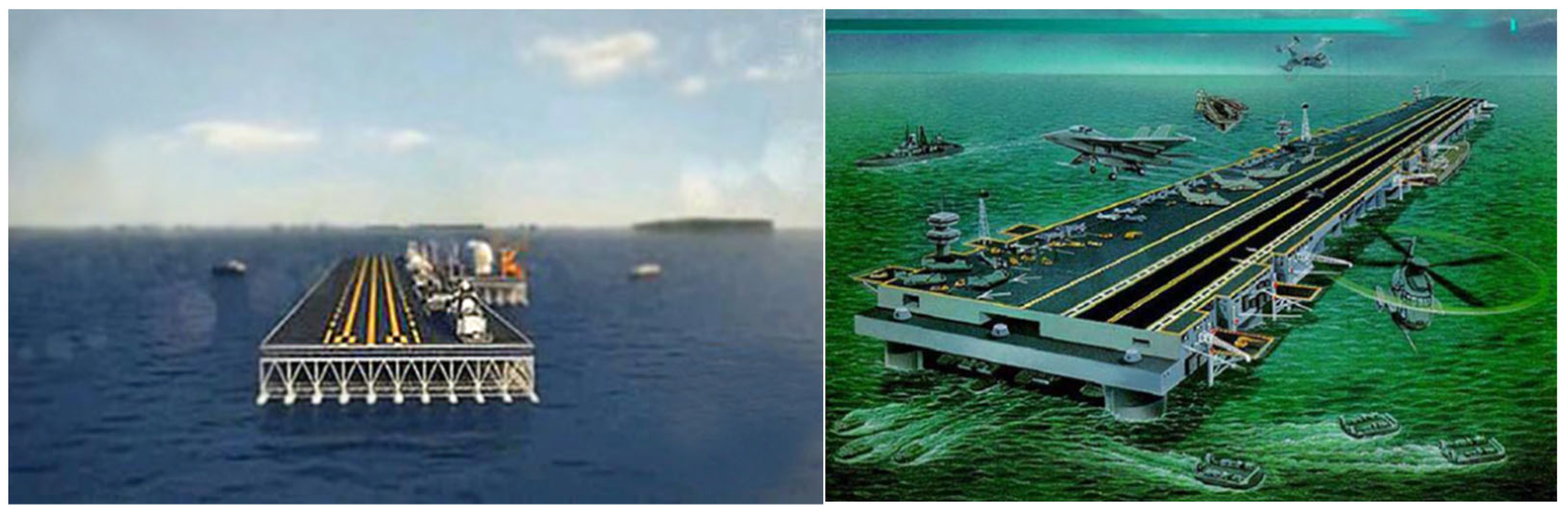
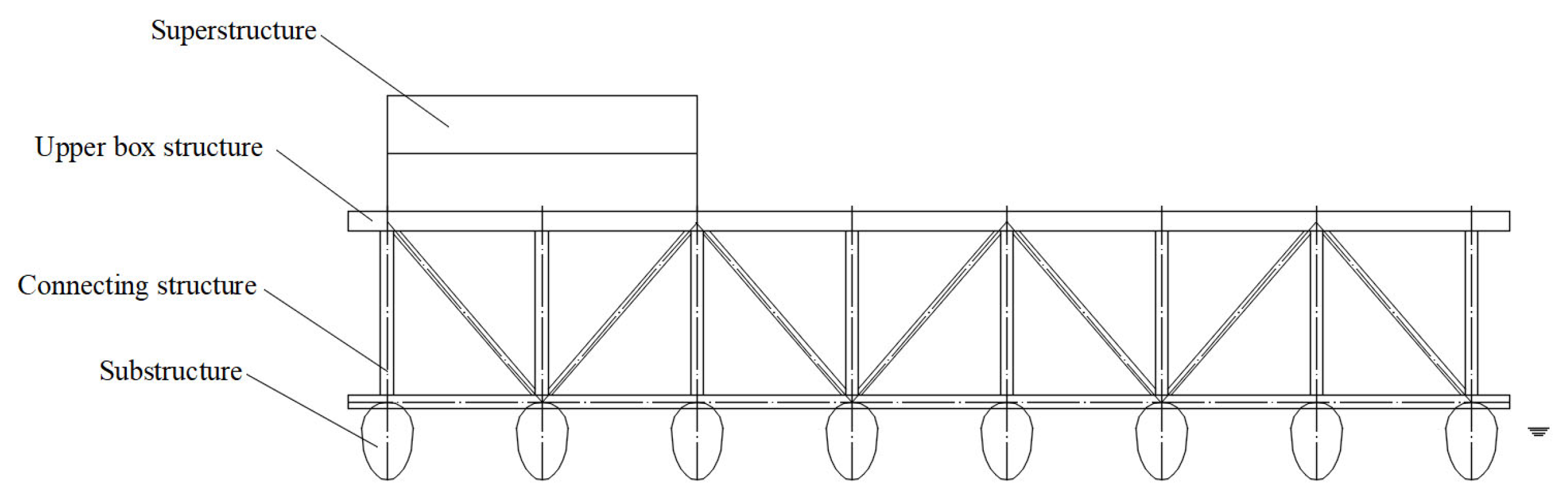
At present, offshore structures tend to increase in dimension and complexity. The so-called large multi-body floating offshore structure shown in Figure 1 and Figure 2 is a new type of floating offshore structure which has appeared in recent years, which is mainly composed of a substructure, connecting structure (truss or column), upper box structure, and superstructure. The substructure is composed of a row of distributed floating bodies. The length and width of the floating offshore structure are very large, while the height is very small. It is an extremely flat and flexible structure. Its stiffness and vibration natural frequency are low, and the elastic deformation cannot be neglected. The calculation of the floating body as a rigid body may greatly underestimate the bending moment [1]. In addition, under the wave action of multiple floating bodies, the reflected wave of a floating body will affect the motions and loads on other floating bodies, and waves will be amplified or sheltered in some areas. The fluid flow around the floating bodies is very complex, especially when the spacing between dispersed floating bodies is small and the fluid resonates inside the spacing. In addition, the viscous effect is also obvious, which makes it particularly difficult to predict the motions and loads of floating bodies. Since the size of a single floating body in the substructure is relatively small, strong nonlinear phenomena, such as wave overtopping the floating body and the water entry and exit of the floating body, will occur under severe sea conditions. Therefore, it is necessary to analyze the deformation of this large-scale offshore structure under fluid loads and the influence of floating body deformation using nonlinear hydroelastic methods accounting for the fluid viscosity, so as to obtain the wave loads and structural responses. According to the results of the tank model test, the deformation and displacement of each floating body are consistent at each time in head seas. Therefore, in order to reasonably reduce the difficulty and complexity and also to focus on the main problems, the present study chose to analyze the hydroelastic behavior of a single body instead of an entire floating structure and verify the feasibility of the CFD-FEA coupling method. The large multi-body floating offshore structure has many usages. The floating offshore structure of a length of 300 m is an independent and complete module, i.e., a module of a 300 m long structure alone can also be used as a floating port; in this case, a single module can be analyzed. If a larger length is required, such as that used as a floating airport, several modules can be connected by connectors. In the case of a large floating structure comprising of several modules, it is still reasonable and appropriate to start with the hydroelastic analysis of a single module.

Since the late 1970s, the potential-flow-based theory and methods for hydroelasticity analysis have made remarkable progress. Betts et al. [2] proposed a two-dimensional hydroelasticity theory. Wu [3] devised a fully three-dimensional approach using a generalized boundary condition of the fluid–solid interface, and the method has been very successful and widely applied in the community. However, the limitations of the methods based on potential flow theory are also obvious. Compared with potential-flow-based theory, CFD (computational fluid dynamics) methods are more accurate in describing the changes in velocity and pressure in the fluid domain, capturing the nonlinear phenomenon of waves on the free surface, and simulating the fine flow field with hydrodynamic interactions between multiple bodies. Xie et al. [4], Wang and Guedes Soares [5], Jiao and Huang [6], Huang et al. [7], and Jiao et al. [8] applied CFD-based methods to analyze the seakeeping and wave loads of ships and offshore structures. It has been found that, compared with potential-flow-based methods, CFD methods can more realistically simulate the flow field and obtain more accurate numerical results.

In recent years, with the development of CFD technology and the improvement of computer performance, some researchers have begun to study how to couple CFD (computational fluid dynamics) and FEA (finite element analysis) for hydroelasticity analysis. El Moctar et al. [9] and Oberhagemann [10] combined the CFD method and the Timoshenko beam model for a two-way coupling simulation of ship slamming loads, and validation against the experimental results was also conducted. Because the Timoshenko beam model is relatively simple, only vertical bending and horizontal bending were studied, thus it is not applicable to the torsion problem. Wilson et al. [11] used a CFD method to study the flow of a ship in waves, and then applied the motions and pressure distribution on the ship’s hull to the finite element model of the ship’s structure for a structural analysis. In order to reduce the amount of calculation, only a one-way coupling method was adopted, i.e., only the influence of fluid on the structure was considered, while the influence of structural deformation on the fluid was neglected. Liu et al. [12] developed a CFD-FEM (computation fluid dynamics–finite element method) coupling simulation method for estimating the hydroelastic responses of the floating elastic plate. For offshore structures with complex forms, the finite element model for the entire hull structure would also be very complex, thus the amount of time required for the fluid–structure coupling calculation would be very large and result in great difficulties in practical applications. Lakshmynarayanana and Hirdaris [13] and Lakshmynarayanana and Temarel [14] studied the symmetrical motions and loads of the S175 container ship in severe waves and under slamming impacts using one-way and two-way CFD-FEA coupling methods. It was shown that the two-way coupling method is able to more accurately estimate the hydroelastic effects of ships in waves. Jiao et al. [15] used the two-way CFD-FEA coupling method to predict the motions, wave loads, and hydroelastic responses of the S175 container ship in regular waves. All the methods adopted in [13,14,15] are based on the linear Timoshenko beam element to simplify the simulation of the hull structure, neglecting the influence of rotational inertia on the motions and wave loads of offshore structures. This simplification is acceptable for the case of head seas, but not for quartering and beam seas as the effect of rotational inertia is significant and cannot be completely neglected.

To sum up, the existing hydroelastic analysis methods have certain limitations, and there are still some difficulties in calculating the wave loads on the large multi-body floating offshore structure shown in Figure 1. Previous studies focused on traditional ships, such as barges or container ships. Although traditional ship types can also reach 300 m in length, due to the differences in structural forms, the hydrodynamic and structural response characteristics are different. The hydroelastic analysis method for traditional ship types may not be well suited for large multi-body floating offshore structures. For instance, wave overtopping on the structure is a phenomenon that may behave differently between the two types of structures. To capture such behaviors with complex phenomena, the CFD-FEA coupling method, for its inherent natures of methodology, is a possible solution.

In this study, a CFD-FEA coupling simulation approach is devised, where the fluid domain is solved by the RANS (Reynolds-averaged Navier–Stokes)-based commercial code STAR-CCM+ [16], and the structure domain is solved by the commercial FE code ABAQUS [17]. The advantage of this method is that it can fully consider the interaction between elastic structure and fluid through two-way fluid–structure coupling and it can effectively solve strong nonlinear problems such as wave overtopping the floating body and water entry and exit of the floating body. At the same time, it can significantly reduce the computational time of the fluid–structure coupling calculation, and it is applicable to the case of head seas, quartering seas, and beam seas. It is suitable for solving the nonlinear wave loads of large multi-body floating offshore structures accounting for the influence of hydroelasticity. In the present study, a single floating body of the large multi-body floating offshore structure as shown in Figure 1 is studied, and the hydrodynamic and structural response characteristics of a single floating body of the large multi-body floating offshore structure are studied with a CFD-FEA coupling method. By comparing the potential-flow-based numerical results for wave loads with and without accounting for the elasticity, the CFD-FEA-based method for hydroelastic analysis of flexible floating structures is validated. It is found that the CFD-FEA method has the potential to capture the complex phenomena of the wave–structure interaction.

The paper is organized as follows: the problem and method of solution used in this study are described in Section 2. Then, in Section 3, the numerical modeling and mesh sensitivity analysis are carried out with the verification of the numerical method. In Section 4, the numerical method is validated by comparing the potential-flow-based numerical results for wave loads with and without accounting for the elasticity. Finally, the conclusion is drawn in Section 5.

2. Problem Statement and Method of Solution

2.1. Problem Statement

In the wave loads on a single floating body of the large multi-body floating offshore structure, the nonlinear factors of the hydrodynamic problem are significant, such as the instantaneous position variation in the body surface, the nonlinearity of the free surface, the elastic deformation of the floating body. These nonlinear factors have a great influence on the loads and motions of the floating body. In order to account for the nonlinear factors, a two-way fluid–structure simulation approach is adopted by coupling CFD and FEA. The fluid domain is solved using the finite volume method (FVM) using STAR-CCM+, and the structure domain is solved by the finite element method (FEM) using ABAQUS.

For the fluid domain, according to Park et al. [18], the contribution of the compressibility and surface tension of the fluid is small and can be neglected. The mass conservation equation and Navier–Stokes equation are used to describe the flow of viscous fluid:

$$\nabla \cdot v=0$$

(1)

$$f-\frac{1}{\rho }\nabla p+\mu {\nabla }^{2}v=\frac{\partial v}{\partial \mathrm{t}}+\left(v\cdot \nabla \right)v$$

(2)

where $p$ is the fluid pressure, $v$ is the velocity vector, $\rho$ is the fluid density and $\mu$ is the dynamic viscosity, and $f$ is the gravity.

For the structure domain, assuming that the structure is a linear elastic material, the motion equation of the structure is obtained using the finite element method:

$$\left[M\right]\left\{\ddot{u}\right\}+\left[C\right]\left\{\dot{u}\right\}+\left[K\right]\left\{u\right\}=\left\{F\right\}$$

(3)

where $\left[M\right]$ is the mass matrix of the structure, $\left[C\right]$ is the damping matrix of structure, $\left[K\right]$ is the stiffness matrix of the structure, $\left\{F\right\}$ is the external fluid loads from the CFD solution in the fluid domain, including the fluid pressure and shear force, and $\left\{u\right\}$ is the motions and deformations of the structure.

2.2. Coupling Approach

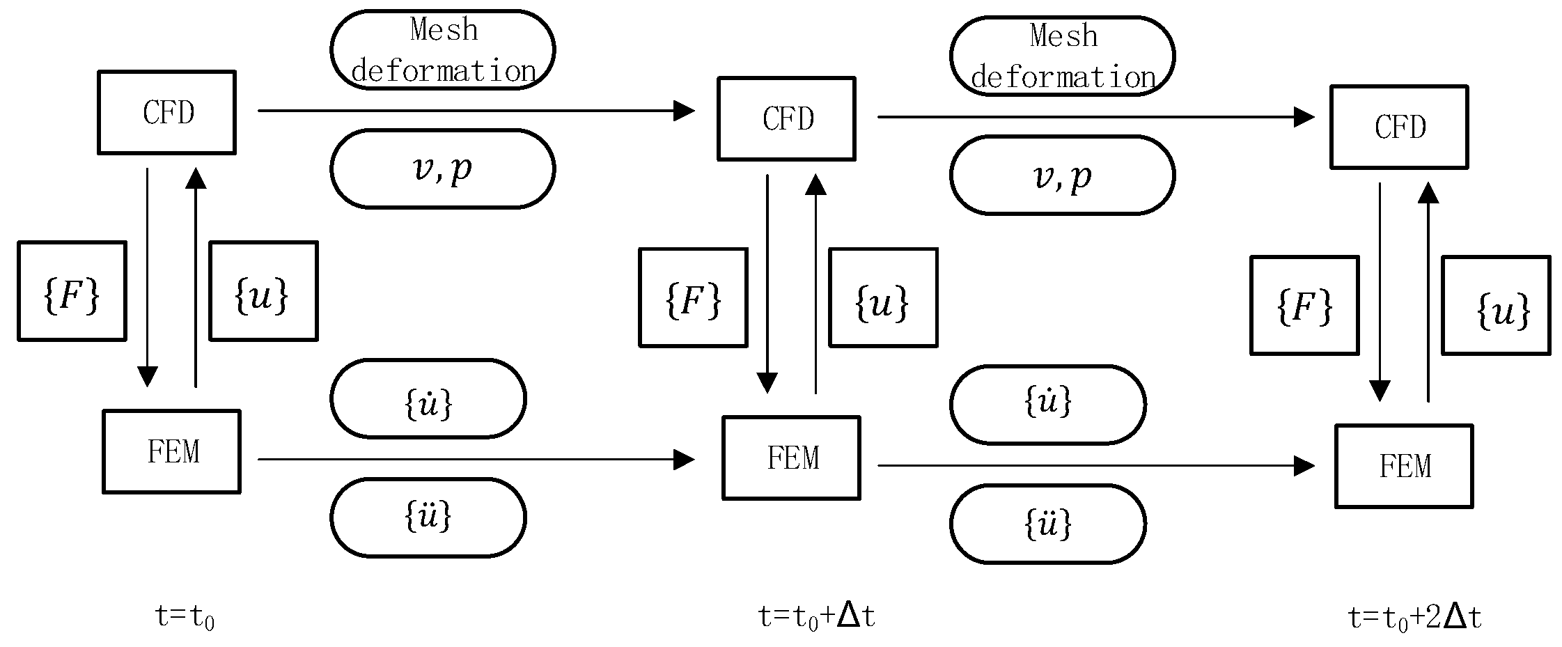
The coupling approach is shown in Figure 3, where $t_0$ is the initial time and $\Delta t$ is the time step. At the initial time, the finite volume method (FVM)-based code STAR-CCM+ is used to calculate the fluid pressure and shear force on the floating body surface, and then the quantities obtained by the FVM are applied to the floating body surface in the finite element model in ABAQUS by means of data mapping. Under the action of fluid pressure and shear force in the fluid domain, the velocity and acceleration of the finite element nodes of the floating body will vary, which leads to the motions and deformations of the fluid–structure coupling interface. Then, the node displacements are transferred to STAR-CCM+ to update the coupling interface. The pressure field and velocity field obtained by STAR-CCM+ are then transferred to the next time step, as well as the velocity and acceleration of the nodes obtained by ABAQUS.

2.3. Coordinate Systems

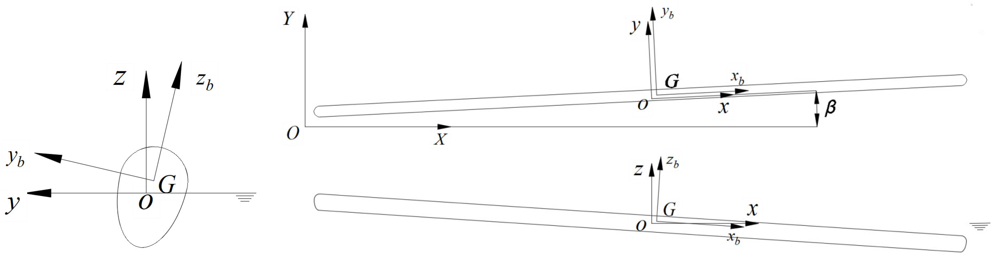
Three right-handed orthogonal coordinate systems are used to describe the floating body motions: earth-fixed coordinate system $O-XYZ$, body-fixed coordinate system $G-x_b{y}_b{z}_b$, and steadily translating coordinate system $o-xyz$.

The origin of the earth-fixed coordinate system $O-XYZ$ lies on the still water surface. The positive $X$ axis is in the direction of the wave propagation, the positive $Z$ axis is directed upwards, and $\beta$ is the wave direction, as shown in Figure 4.

The body-fixed coordinate system $G-x_b{y}_b{z}_b$ is connected to the ship, with its origin placed at the center of gravity $G$. The positive $x_b$ axis is in the longitudinal forward direction. The positive $y_b$ axis is pointing in the port side direction. The positive $z_b$ axis is perpendicular to the waterline of the hull and is pointing upward.

The steadily translating coordinate system $o-xyz$ is moving forward at the nominal speed. If the floating body is stationary, the origin of the coordinate system $o-xyz$ is located at the intersection of the still water surface, the midship cross-section and the center plane, and the directions of the $o-xyz$ axes are the same as those of the $G-x_b{y}_b{z}_b$.

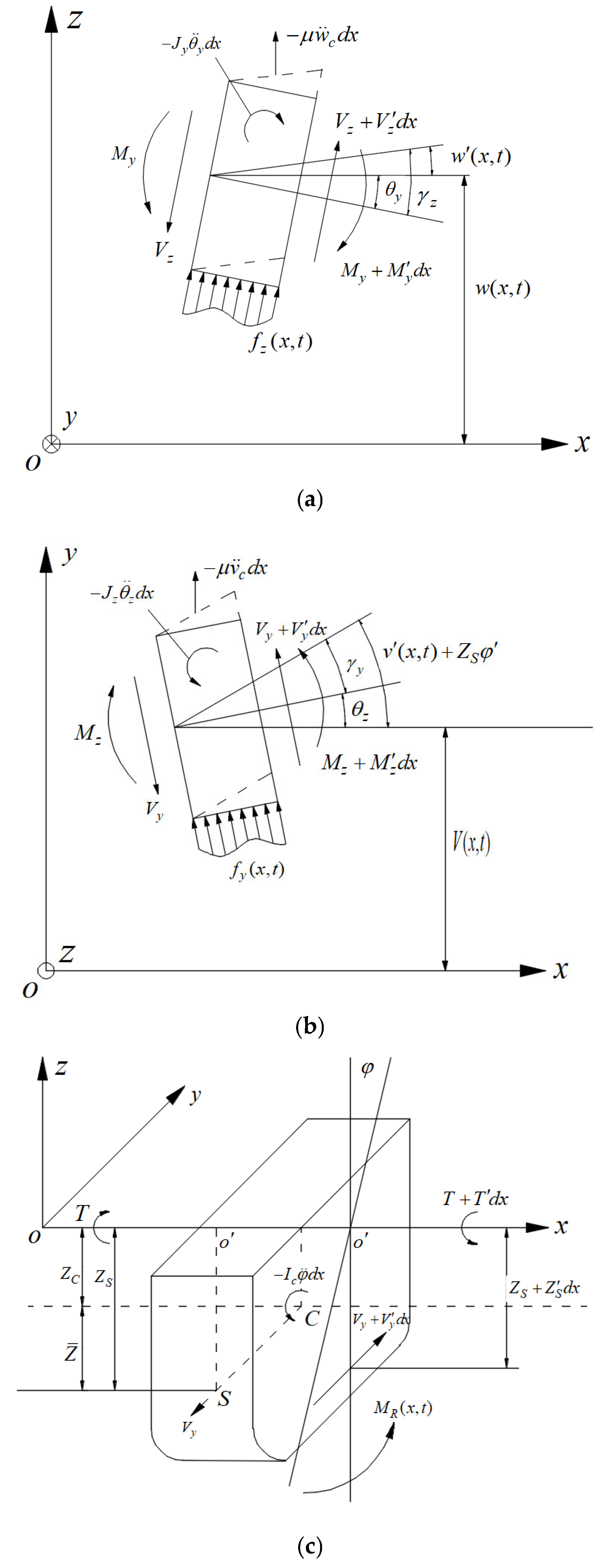
2.4. Backbone Beam

A backbone beam is used to simulate the stiffness of the whole floating body. The stress and deformation of the micro-segment of the backbone beam are analyzed. The micro-segment of the backbone beam is shown in Figure 5 [19]. The beam is located in the $o-xyz$ coordinate system. As shown in Figure 5c, the reference point $o^{\prime }$ is the intersection of the $ox$ axis and the cross-section of the micro-segment when floating still, i.e., the intersection of $G{x}_B$ axis and section of the micro-segment. In Figure 5c, $C$ is the mass center of the micro-segment; $S$ is the shear center of the micro-segment; $Z_C(x)$ is the distance between the mass centroid $C$ and $o^{\prime }$; $Z_S(x)$ is the distance between the shear center $S$ and $o^{\prime }$; and $\overline{Z}(x)$ is the distance between the center of mass $C$ and the shear center $S$, $\overline{Z}(x)=Z_S(x)-Z_C(x)$.

For the vertical bending, as shown in Figure 5a, the differential equations of the motion of the backbone beam are:

$$\left\{\begin{array}{l}\mu \left(x\right)\ddot{w}(x,t)=V_z^{\prime }(x,t)+f_z(x,t)\\ J_y\left(x\right){\ddot{\theta }}_y(x,t)=M_y^{\prime }(x,t)-V_z(x,t)\end{array}\right.$$

(4)

For the horizontal bending and torsion, as shown in Figure 5b,c, the differential equations of the motion of the backbone beam are:

$$\left\{\begin{array}{l}\mu \left(x\right){\ddot{v}}_c(x,t)=V_y^{\prime }(x,t)+f_y(x,t)\\ J_z\left(x\right){\ddot{\theta }}_z(x,t)=M_z^{\prime }(x,t)+V_y(x,t)\\ I_c(x)\ddot{\phi }(x,t)=T^{\prime }(x,t)+\overline{Z}(x)V_y^{\prime }(x,t)+Z_S^{\prime }(x)V_y(x,t)+M_R(x,t)\end{array}\right.$$

(5)

where $\mu \left(x\right)$ is the mass distribution per unit length of the beam; $J\left(x\right)$ is the moment of inertia per unit length of the beam; $I_c$ is the torsional moment of inertia per unit length passing through the mass center $C$ and parallel to the $G{X}_b$ axis, and its relationship with the moment of inertia $I_O(x)$ about the $G{X}_b$ axis is $I_o(x)=I_C(\mathrm{x})+Z_C^2(x)\mu (x)$; $w\left(x,t\right)$ is the vertical bending deformation of the cross-section center; $\theta \left(x,t\right)$ is the rotation angle of the section due to bending; $\phi \left(x,t\right)$ is the rotation angle of the cross-section due to torsion; $f$ is the force acting on the unit length of the beam; $M\left(x,t\right)$ is the cross-section bending moment; $V\left(x,t\right)$ is the cross-section shear force; $T\left(x,t\right)$ is the cross-section disturbing force; and $M_R\left(x,t\right)$ is the roll moment acting on the unit length of the beam. The subscript $y$ denotes the $y$ direction or rotating about the $y$ axis, and the subscript $z$ stands for the $z$ direction or rotating about the $z$ axis. The dot over the variable denotes the time derivative, and the prime indicates the partial derivative of the length $x$.

According to the Timoshenko beam theory, the relationship between the force and deformation on the section can be obtained as below. For the vertical bending,

$$\left\{\begin{array}{l}{V}_z(x,t)=kG{A}_V(x)\left[{\gamma }_z(x,t)+{\alpha }_V(x){\dot{\gamma }}_z(x,t)\right]\\ M_y(x,t)=E{I}_V(x)\left[{\theta }_y^{\prime }(x,t)+{\beta }_V(x){\dot{\theta }}_y^{\prime }(x,t)\right]\end{array}\right.$$

(6)

For the horizontal bending and torsion,

$$\left\{\begin{array}{l}{V}_y(x,t)=kG{A}_H(x)\left[{\gamma }_y(x,t)+{\alpha }_H(x){\dot{\gamma }}_y(x,t)\right]\\ M_z(x,t)=E{I}_H(x)\left[{\theta }_z^{\prime }(x,t)+{\beta }_H(x){\dot{\theta }}_z^{\prime }(x,t)\right]\\ T(x,t)=C(x){\phi }^{\prime }(x,t)-{\left[C_l(x){\phi }^{″}(x,t)\right]}^{\prime }+\mathrm{\Gamma }(x){\dot{\phi }}^{\prime }(x,t)\end{array}\right.$$

(7)

where $kGA$ is the shear stiffness of the section; $EI$ is the bending stiffness of the section; $C$ is the torsional stiffness of the section; $\alpha$ is the shear damping coefficient; $\beta$ is the bending damping coefficient; $\mathrm{\Gamma }$ is torsional damping coefficient; $\gamma$ is the shear angle; and $C_l$ is the warping stiffness. Subscripts $V$ and $H$ indicate that the quantities are related to a vertical or horizontal motion, respectively.

The geometric relationship of the deformation of the backbone beam is:

$$w^{\prime }(x,t)={\gamma }_z(x,t)-{\theta }_y(x,t)$$

(8)

$${\left[v(x,t)+Z_S(x)\phi (x,t)\right]}^{\prime }=Z_S^{\prime }(x)\phi (x,t)+{\gamma }_y(x,t)+{\theta }_z(x,t)$$

(9)

In the above Equations (4), (6) and (8) constitute the governing equations of vertical motion, and (5), (7) and (9) constitute the horizontal motion and torsional motion of the backbone beam.

2.5. Section Loads Calculation

Through the above calculation, the pressure distribution, velocity, and acceleration on the surface of the floating body can be obtained, and then the forces and moments at the cross-section of the floating body can be calculated according to the following formula [20].

$$\left\{\overline{Q}\right\}=-\underset{S_x}{\iint }P\left\{n\right\}ds+\left[M\right]g-\left[M\right][\ddot{\mu }]+\left\{\Delta \overline{Q}\right\}$$

(10)

where $\left\{\overline{Q}\right\}={\left(N S{F}_Y S{F}_Z TM B{M}_Y B{M}_Z\right)}^T$ is the six-component of the section loads, $S_x$ is the wetted surface area of a floating body over a partial length, $P$ is the total fluid pressure and shear force, $\left\{\Delta \overline{Q}\right\}={\left(0 0 0 0 x\cdot S{F}_Z-x\cdot S{F}_Y\right)}^T$ is the additional item, $\left[M\right]$ is the mass matrix of the partial length floating body, and $\left[\ddot{\eta }\right]$ is the 6-DOF acceleration of the floating body.

3. Numerical Modeling and Simulation

In this section, the numerical modeling is introduced. Then, the extent of the computational domain, boundary condition, time step, and mesh sensitivity analysis are discussed and analyzed, and the numerical method is verified.

3.1. Numerical Modeling

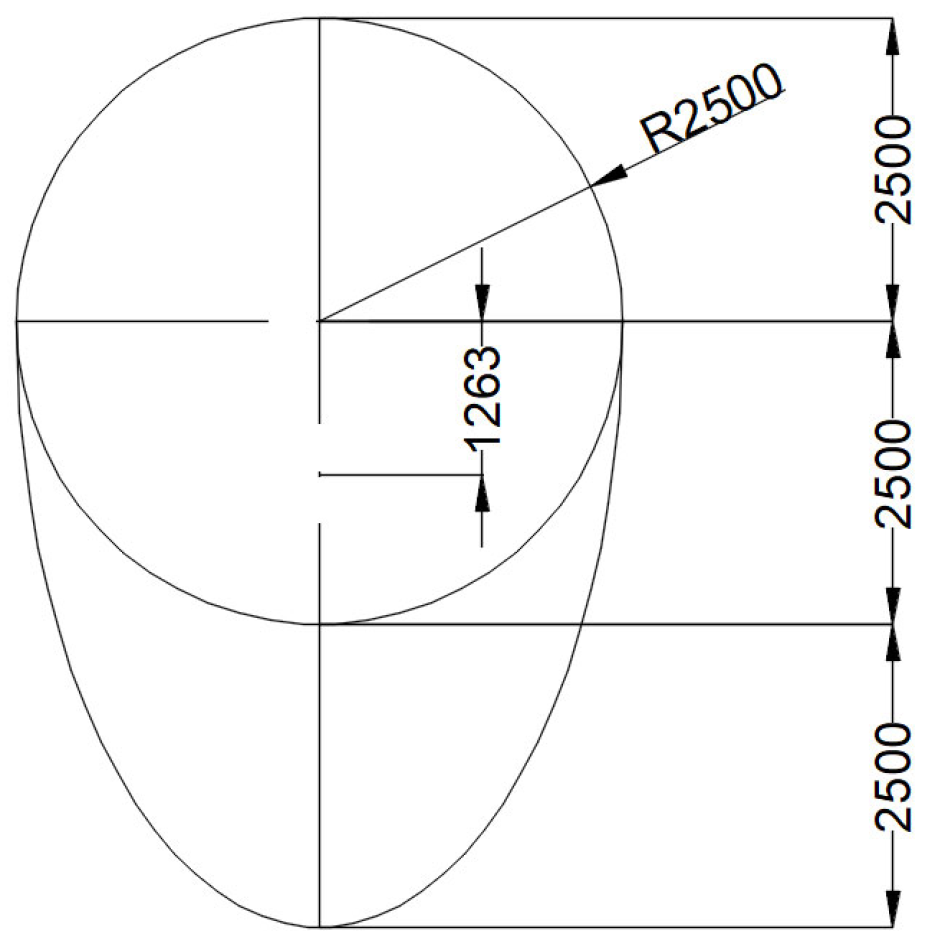
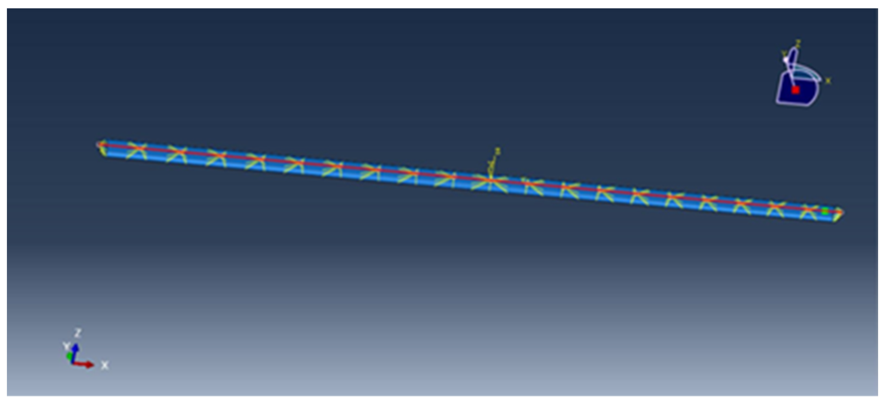
The length of a single floating body of large multi-body floating offshore structure is 300 m, the height is 7.5 m, the width is 5 m, the draft is 5 m, and the mass is evenly distributed along the length of the single floating body. The transverse cross-section of the single floating body is shown in Figure 6, and the thickness of the single floating body plate is 20 mm. The hollow rectangular beam is used as the backbone beam to simulate the stiffness of the whole floating body. The floating body has 21 stations (0–20 stations) in total, and is divided into 20 sections, as shown in Figure 7. The red line in Figure 7 denotes the backbone beam.

The vertical bending stiffness and longitudinal torsional stiffness of the actual floating body cross-section and backbone beam are shown in

Table 1. Stiffness parameters.

	Symbols	Units	Actual Value	Backbone Beam	Deviation
Moment of inertia	$I_y$	${\mathrm{m}}^4$	2.61	2.60	−0.30%
Torsional moment of inertia	$I_n$	${\mathrm{m}}^4$	3.74	3.74	0.10%
Vertical bending stiffness	$E{I}_y$	$\mathrm{N}\cdot {\mathrm{m}}^2$	5.37 × 1011	5.35 × 1011	−0.30%
Longitudinal torsional stiffness	$G{I}_n$	$\mathrm{N}\cdot {\mathrm{m}}^2$	2.96 × 1011	2.97 × 1011	0.10%

.

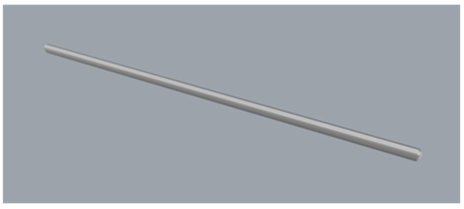
The single floating body of a large multi-body floating offshore structure is shown in Figure 8. The structural model is composed of two parts, the hull surface and the backbone beam, as shown in Figure 9. The hull surface of the floating body is modeled using shell elements, denoted by the blue surface in Figure 9. The hull surface is the fluid–structure coupling interface, where the external fluid loads are mapped from the fluid domain, which makes no contribution to the overall stiffness and mass of the floating body. The backbone beam is simulated by three-dimensional Timoshenko beam elements, denoted by the red line in Figure 9, which contributes to the stiffness, mass, and moment of the inertia of the floating body. The beam elements are connected to the shell elements by kinematic coupling constraints. The CFD solutions for the external fluid loads in the fluid domain are transferred to the FEA model in the structure domain through the hull surface for structural dynamic analysis. Once the structural dynamic analysis is done, the solutions for the motions and deformations of the backbone beam are obtained. Because of the kinematic coupling constraints between the beam elements and the shell elements, the motions and deformations of the backbone beam will also be fed back to the hull surface for the subsequent hydrodynamic analysis in the fluid domain.

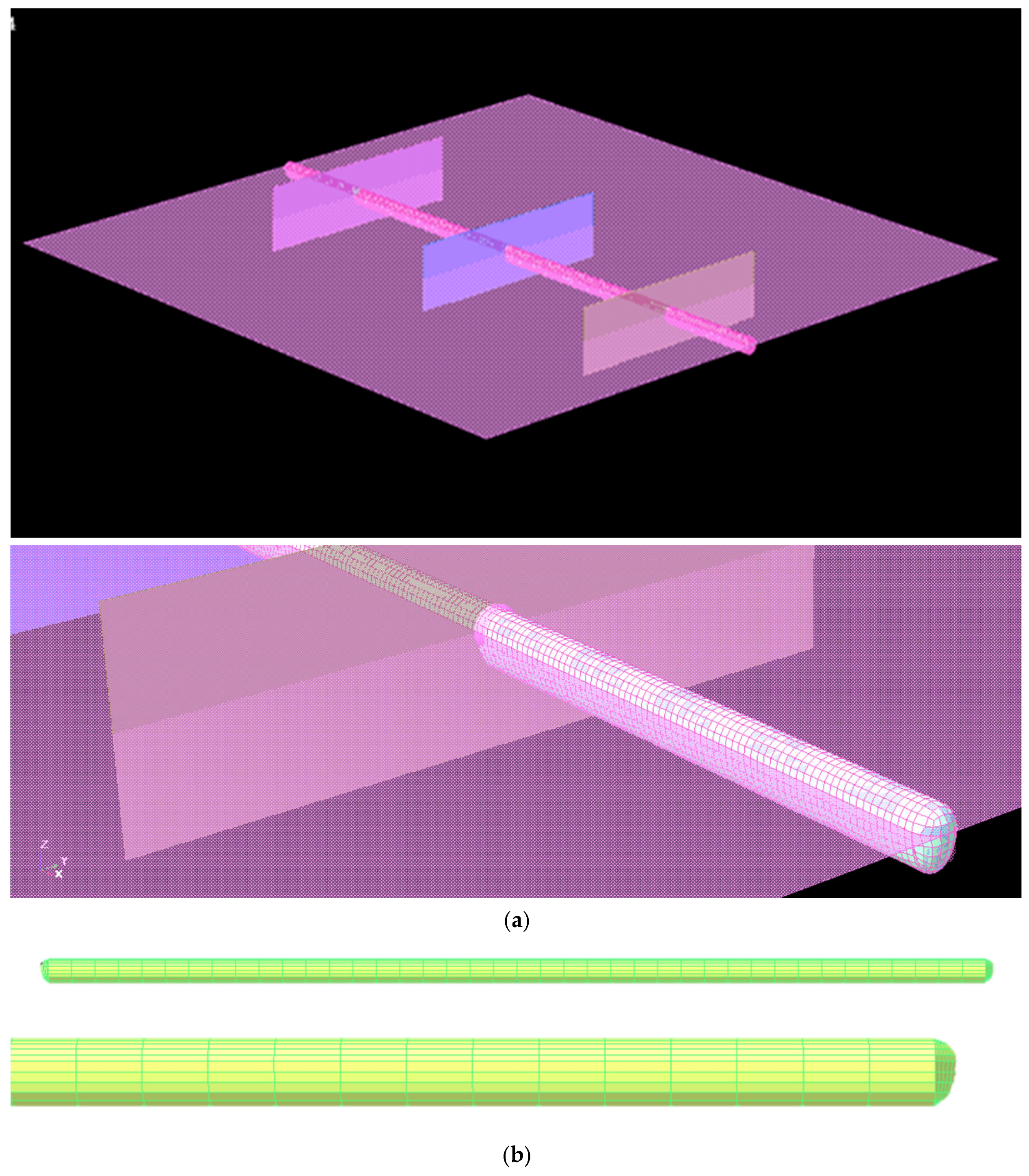
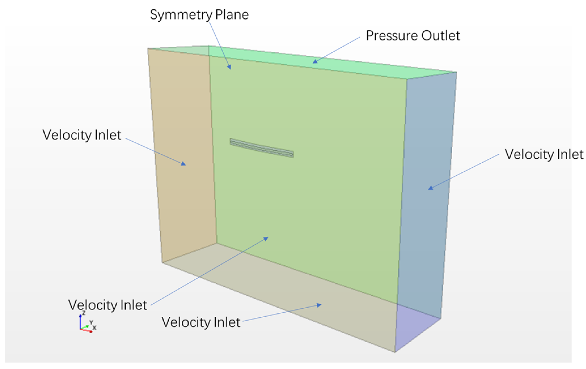
The fluid domain modeling and mesh generation are carried out in STAR-CCM+. The wavelength is set to be L, the length and width of the fluid domain are 4L, the distance between the static water surface and the bottom of the domain is 2L, and the distance between the static water surface and the top is 2L. The boundary conditions are set [8,21] as shown in Figure 10. A pressure outlet is applied at the top boundary. The nonslip wall boundary condition is applied at the floating body surface. Since the floating body is a symmetrical structure, and so is the flow about it in head seas, only half of the flow field needs to be simulated. The symmetry plane boundary condition is applied at the center plane of the structure. Regarding the other four boundary planes, the velocity inlet is applied, where the velocity of the wave is prescribed to avoid the gradient generated from the wall and flow [21]. 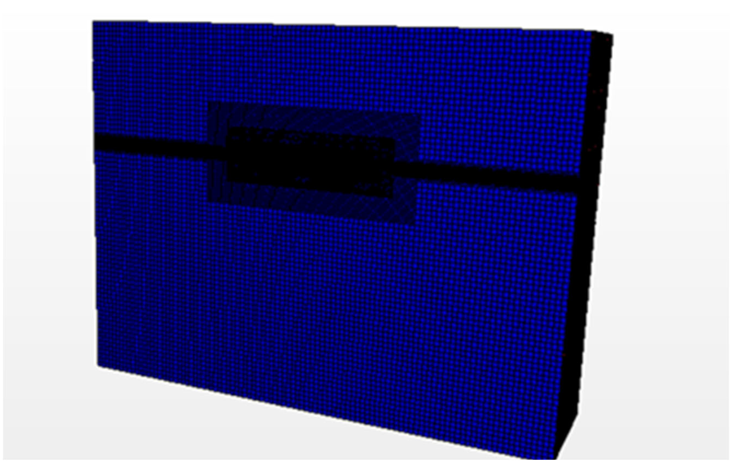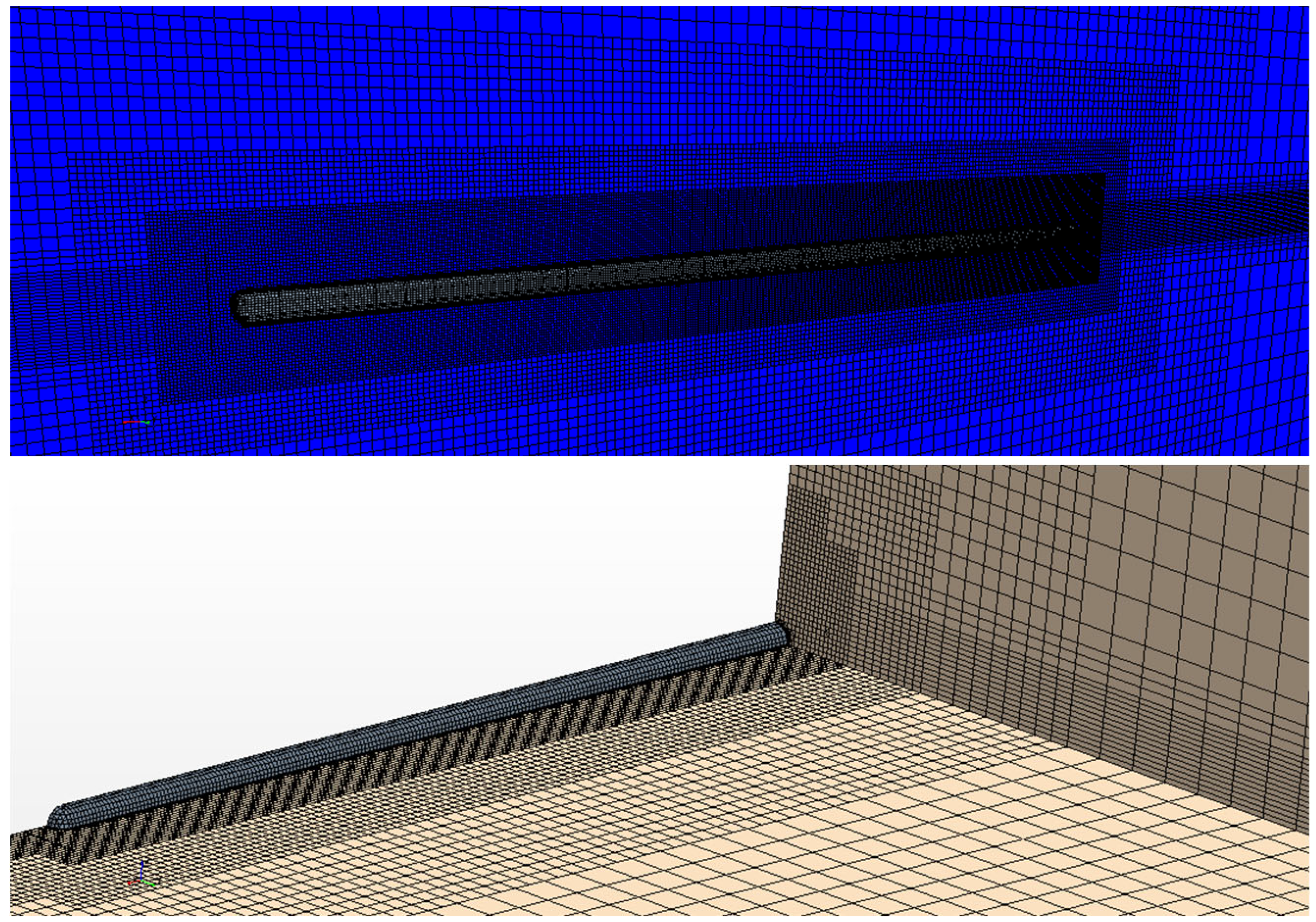The volume of fluid (VOF) method is used to track free surfaces at the interface between air and water [22]. The fluid domain is meshed as shown in Figure 11. The extent of the whole computational domain is determined by referring to the recommendations of ITTC [23]. The distance between the bow of the floating body and the inlet boundary is 1.5L, and the distance between the stern of the floating body and the outlet boundary is also 1.5L. The FVM is used to solve the fluid domain, and the fluid pressure and shear force on the surface of the floating body are obtained. The direction of the force due to the pressure is perpendicular to the surface of the floating body, and the direction of the shear force is tangent to the surface of the floating body.

The Courant number is used to evaluate the time step requirements of a transient simulation for a given mesh size and flow velocity.

$$C=\frac{U\Delta t}{\Delta x}$$

(11)

where $C$ is the Courant number, $U$ is the flow velocity, $\Delta t$ is the representative time step of the simulation, and $\Delta x$ is the characteristic size of the mesh cell.

In order to ensure the accuracy and stability of the numerical results, the Courant number should be less than one [24]. A constant time step of 0.01 s is chosen for the simulations.

The long-crest regular waves are created using linear airy wave theory. Since the offshore structure is in a moored condition during the operation, the forward speed is set to zero in the simulation. In head seas, the heave and pitch motions of the floating body are released, while the surge motion is constrained. Additionally, because of the symmetry, only half of the flow field is simulated, and a symmetrical boundary condition is applied at the center plane, that is, there are no sway, roll, and yaw motions.

3.2. Mesh Sensitivity Analysis

For the mesh convergence analysis, three sets of meshes, as shown in

Table 2. Three sets of meshes.

Mesh	Minimum Size of Fluid Domain			Base Size of Structure Domain	Number of Meshes
	x	y	z
Mesh A	1.56 m	6.00 m	6.00 m	1.50 m	0.8 million
Mesh B	0.78 m	6.00 m	6.00 m	0.75 m	1.5 million
Mesh C	0.24 m	0.24 m	0.24 m	0.50 m	5.2 million

, are generated for the structure domain and fluid domain mentioned above. A regular wave of 300 m in wave length and 16 m in wave height is used for the mesh sensitivity analysis.

The accuracy of the wave simulation is very important for the accuracy of the simulation of floating body’s motions and loads. According to the recommendation by STAR-CCM+, which has also been validated by many researchers [25], a minimum of 40 cells per wavelength and 20 cells per wave height on the free surface is necessary to produce a stable wave with an acceptable dissipation. The mesh created according to the principle is Mesh B, as shown in Table 2, and the mesh which is relatively coarser is Mesh A, while the mesh which is relatively coarser is Mesh C.

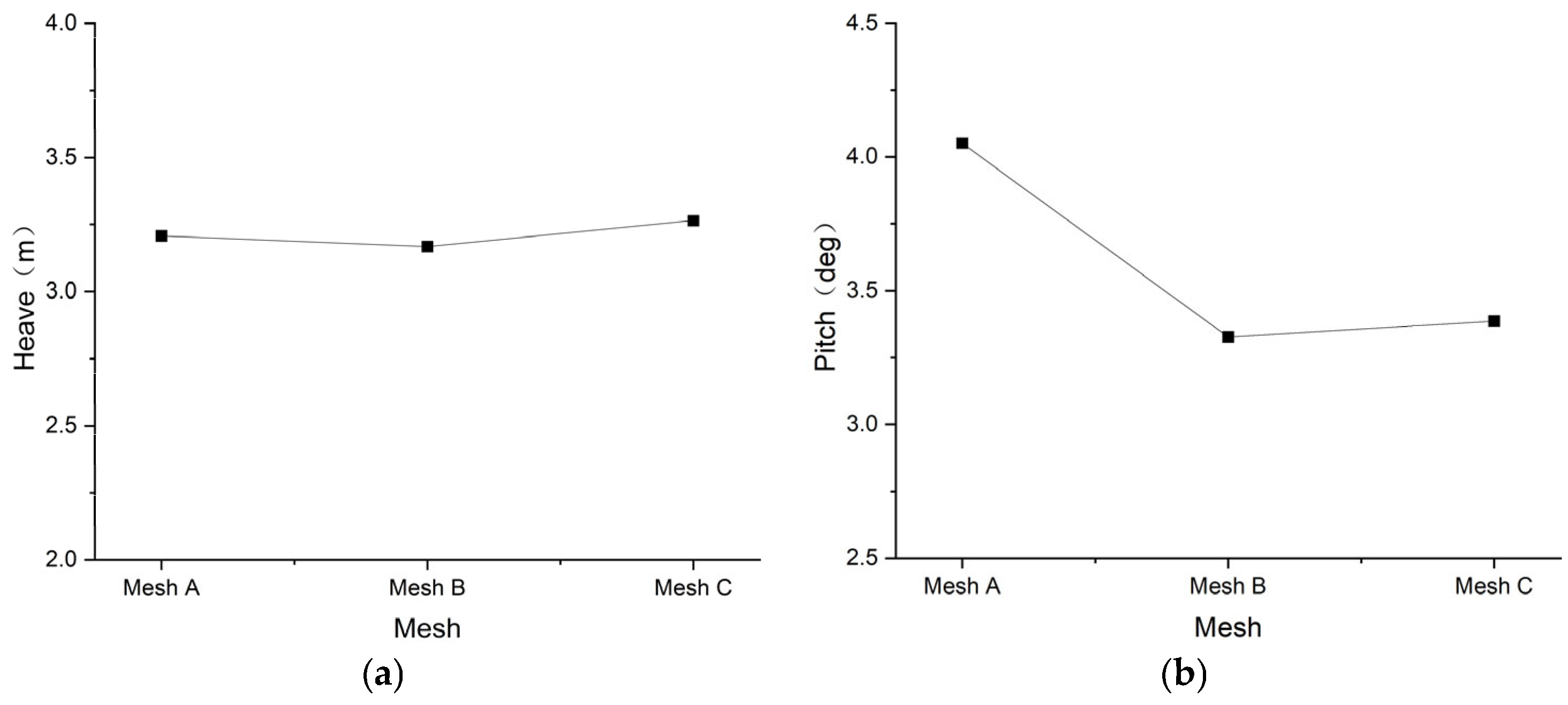
The numerical results for the amplitudes of the heave and pitch motion of the single floating body are presented in Figure 12. The values of the heave and pitch motion are only rigid body displacements and do not include the elastic deformations of the floating body. For the heave motion, the results obtained with the three sets of meshes are very close to each other. For the pitch motion, the results obtained with Mesh B are very close to that obtained with Mesh C, with an average difference of 1.7%, but there is a relatively large difference, 21%, between the results obtained with Mesh A and Mesh B.

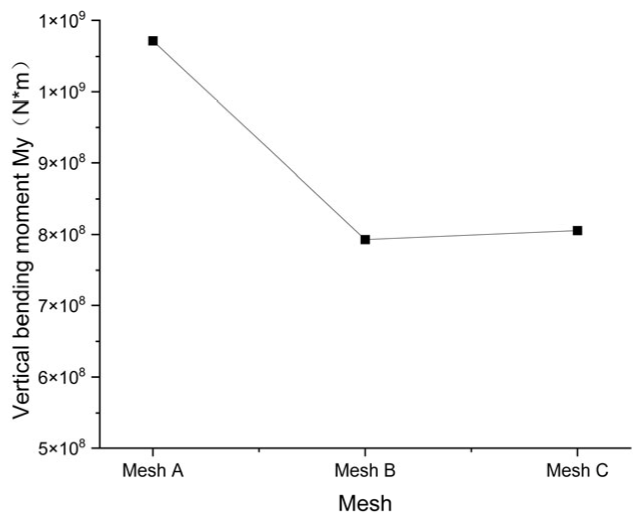
The numerical results for the amplitudes of the vertical bending moment at midship are presented in Figure 13. Mesh B and Mesh C produce similar results, and the average difference between them is 1.6%. In comparison, there is a relatively large average difference, 35%, between the results obtained with Mesh A and Mesh B.

From the comparison of the results of three sets of meshes, it is found that the results from Mesh B and Mesh C are very close to each other, which shows the good mesh convergence property of the numerical model. Mesh B, with the meshing principle introduced above, is selected in this paper considering the accuracy and efficiency of the calculation.

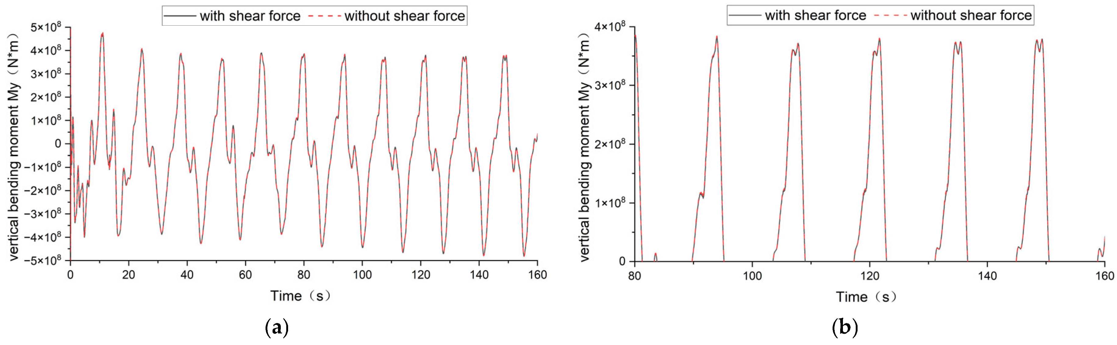
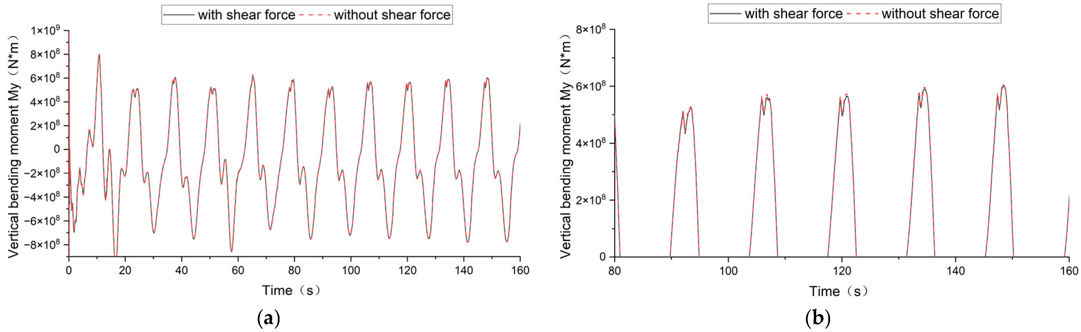
3.3. The Influence of Shear Force along the Wetted Surface

Because the fluid is assumed to be inviscid in potential flow theory, the shear force acting on the wetted surface of the floating body is neglected in SESAM/WADAM [26] and COMPASS-WALCS-NE [27]. As described in Section 2.5, the CFD-FEA method can account for the contribution of the shear force to the global solutions. In order to study the influence of shear force on the vertical bending moment of the cross-section, the numerical results obtained with and without shear force by the CFD-FEA method are compared, as shown in Figure 14 and Figure 15. From the comparison, it can be seen that the influence of shear force on the vertical bending moment of the cross-section is very small.

4. Results and Discussion

In this section, the hydrodynamic and structural responses are obtained using the CFD-FEA method. Then, the results are analyzed and compared with those obtained using a potential-flow-based method for wave loads with and without accounting for the elasticity, and the CFD-FEA method for hydroelastic analysis is validated.

4.1. Numerical Results

The simulation is carried out for a range of regular wave heights, as shown in

Table 3. Regular wave.

Wave Direction	Wave Length	Wave Period	Wave Height
Heading angle 180°	300 m	13.862 s	2.5 m
			5.0 m
			7.5 m
			10.0 m
			12.5 m
			16.0 m

. The results obtained by the CFD-FEA method are compared with those using the commercial code SESAM. In order to investigate the behavior of the numerical simulation without unnecessary repetitions, one of the regular wave heights in Table 3 is chosen as a typical case for in-depth analysis, namely, head seas with a wave height of 16 m.

4.1.1. Wave Simulations

The wave surface elevation of the entire flow field is shown as Figure 16. In Figure 16b, the details of the flow field can be observed clearly, such as water entry and exit of the floating body, elastic deformation of the floating body, and free surface disturbances. Due to the numerical dissipation in the computation and the fluid viscosity, the wave heights are continuously attenuated in the process of wave propagation. In order to verify the accuracy of numerical wave making, several numerical wave height meters are arranged in the flow field to monitor the wave heights at different locations to compare the deviation between the theoretical wave heights and the actual wave heights. The location of numerical wave height meters should be far enough away from the floating body where the influence of the floating body is negligible. Figure 17 shows the actual wave heights at four locations in the flow field. It can be found that the deviations between the actual wave heights and the theoretical wave heights are all within 5%, meeting the accuracy requirements in [25].

4.1.2. Motions and Deformations of the Floating Body in Waves

Figure 18a shows the rigid body displacements and the elastic deformations of the floating body in the vertical direction at four time instants within one wave period. The rigid body displacements of the floating body are removed to obtain the vertical elastic deformation of the floating body at four time instants within one wave period, as shown in Figure 18b. It can be seen that at $t=100 \mathrm{s}$, the floating body is in a sagging condition, and at $t=100 \mathrm{s}+1/2T$, the floating body is in a hogging condition, where $T$ is the wave period.

4.1.3. Wave Loads

The pressure on the floating body surface is shown in Figure 19, and the vertical velocity at the center of gravity of each section of the floating body is shown in Figure 20a. Once the pressure, the vertical velocity, and the vertical acceleration are obtained, the vertical bending moment $M_y$ at the cross-sections of the floating body can be obtained from Equation (5), and the time histories are shown in Figure 20b–d.

It can be seen in Figure 20b–d that the results display a periodic pattern of the wave loads on the floating body under the action of regular waves. In order to analyze the change in the wave loads on the floating body, the flow fields at the instant when the vertical bending moment $M_y$ of the cross-section reaches the peak and the trough are compared. For instance, it can be seen in Figure 20c that at $t=106.84 \mathrm{s}$, $M_y$ at the midship cross-section ($x=0 \mathrm{m}$) reaches a peak value; at $t=113.73 \mathrm{s}$, $M_y$ reaches a trough value. Figure 21 shows the side views of the flow field wave surface at $t=106.84 \mathrm{s}$ and $t=113.73 \mathrm{s}$, respectively. It can be observed in the figures that when the floating body is in a hogging condition, the vertical bending moment $M_y$ at the middle cross-section reaches a peak value, amd when the floating body is in a sagging condition, the vertical bending moment $M_y$ at the middle cross-section reaches a trough value, that is, the location of the wave crest and trough on the floating body causes a hogging or sagging condition of the floating body. As the wave crest and wave trough move longitudinally along the floating body, the vertical bending moment $M_y$ changes with time.

4.1.4. Fluid Pressure

The locations of the fluid pressure monitoring points on the floating body surface are shown in

Table 4. Location of fluid pressure monitoring points.

No. of Fluid Pressure Monitoring Point	Location	Coordinates
		x/m	y/m	z/m
1a	Stern	−147.500	0.000	2.500
1b		−147.500	2.498	0.000
1c		−147.500	2.155	−2.500
1d		−147.500	0.000	−5.000
2a	Midship	0.000	0.000	2.500
2b		0.000	2.498	0.000
2c		0.000	2.155	−2.500
2d		0.000	0.000	−5.000
3a	Bow	147.500	0.000	2.500
3b		147.500	2.498	0.000
3c		147.500	2.155	−2.500
3d		147.500	0.000	−5.000

, and the time history of the pressure is shown in Figure 22. Although it can be seen in the figure that the pressure extrema occur at the bow, midship, and stern of the floating body at some time instants, but no slamming occurred. In Figure 23, it can be found that, in addition to the periodic extrema of the fluid pressure, at some instants, e.g., 111 s, the fluid pressure at the stern of the floating body also has a local extremum. Since the difference in the fluid force between the bottom and top of the stern is approximately equal to the fluid force at the stern of the floating body, the fluid pressure at the top and the bottom of the stern, and the fluid pressure difference between the bottom and the top of the stern, are compared in Figure 23. In Figure 24, it can be found that at 111 s, the fluid pressures at the top and the bottom of the stern have local extrema, and the difference between the bottom and the top of the stern in the pressure also has local extrema. The instant when the fluid pressure at the stern of the floating body reaches a local extremum, the vertical bending moment at the cross-section of the floating body also has a local extremum, as shown in Figure 20b,c.

4.2. Validation of the Numerical Method

In order to validate the CFD-FEA coupling method, the wave loads on a single floating body are computed using the WADAM modules of the SESAM Suite and COMPASS-WALCS-NE, and the numerical results are compared with the CFD-FEA results. SESAM is a well-known suite developed by DNV for the hydrodynamic, structural design, and analysis of ships and offshore structures. WADAM is a module of SESAM developed based on the three-dimensional linear frequency domain potential flow theory. Because of the assumption of a rigid body, the elastic deformation of the floating body is ignored. The factors such as surface nonlinearity, fluid viscosity, and slamming of the floating body cannot be accounted for as well. COMPASS-WALCS-NE is a three-dimensional nonlinear hydroelastic analysis application developed by the China Classification Society. This application is based on the three-dimensional potential flow theory and three-dimensional structural dynamics, taking into account the nonlinear wave force caused by the change in the instantaneous wet surface of the hull, the slamming, and other nonlinear loads, and the influence of the structural elastic deformation on the flow field is also accounted for. COMPASS-WALCS-NE has been validated against experimental results in many studies [28,29,30]; for instance, it has shown that the accuracy of COMPASS-WALCS-NE for nonlinear wave loads is fairly sufficient.

The model used for the simulation with WADAM is shown in Figure 25a, and the one for simulation with COMPASS-WALCS-NE is shown in Figure 25b. During the simulation, the vertical bending moments $M_y$ at the cross-sections of x = −7.5 m, 0 m, and 75 m are monitored.

4.2.1. Comparison with WADAM Numerical Results

The numerical results of CFD-FEA and WADAM are compared in

Table 5. Comparison of calculation results of CFD-FEA and WADAM.

Wave Height/m	Method	Amplitude of Vertical Bending Moment ${\mathit{M}}_{\mathit{y}}$$/\mathbf{N}·\mathbf{m}$
		x = −75 m	x = 0 m	x = 75 m
2.5	CFD-FEA	1.052 × 108	2.087 × 108	1.096 × 108
	WADAM	1.219 × 108	2.286 × 108	1.261 × 108
	Deviation	−13.70%	−8.71%	−13.08%
5.0	CFD-FEA	1.741 × 108	3.430 × 108	1.663 × 108
	WADAM	2.438 × 108	4.573 × 108	2.523 × 108
	Deviation	−28.59%	−24.99%	−34.09%
7.5	CFD-FEA	2.355 × 108	5.018 × 108	2.381 × 108
	WADAM	3.657 × 108	6.859 × 108	3.784 × 108
	Deviation	−35.60%	−26.84%	−37.08%
10.0	CFD-FEA	2.373 × 108	5.212 × 108	2.622 × 108
	WADAM	4.877 × 108	9.145 × 108	5.045 × 108
	Deviation	−51.34%	−43.01%	−48.03%
12.5	CFD-FEA	3.326 × 108	6.756 × 108	3.307 × 108
	WADAM	6.096 × 108	1.143 × 109	6.306 × 108
	Deviation	−45.44%	−40.89%	−47.56%
16.0	CFD-FEA	4.742 × 108	7.928 × 108	3.315 × 108
	WADAM	7.802 × 108	1.463 × 109	8.072 × 108
	Deviation	−39.22%	−45.81%	−58.93%

. It can be seen that, for small wave heights, waves do not overtop the floating body, and the wave loads are small, thus the floating body does not have an obvious elastic deformation. In this case, the CFD-FEA method and WADAM produce similar numerical results for the amplitude of the vertical bending moment $M_y$. However, because the freeboard of the floating body is small, it is easy for the waves to overtop the floating body in case of large wave heights. In this case, the nonlinear characteristics of the instantaneous position variation in the body surface cannot be simply ignored. As the large wave heights result in large wave loads, the floating body will have obvious elastic deformation, and the hydroelastic response becomes significant. The elastic behavior of the body is ignored in WADAM, resulting in a large deviation between the CFD-FEA and WADAM numerical results in the case of large wave heights.

The variation in the numerical results of CFD-FEA and WADAM with the change in wave height is presented in Figure 26a–c. The results obtained with WADAM show that the amplitude of the vertical bending moment $M_y$ increases linearly with the wave height, while the numerical results obtained with CFD-FEA show that the amplitude of the vertical bending moment $M_y$ also increases with the wave height, but at a lower rate. This is because the CFD-FEA method can effectively capture the nonlinear characteristics of an instantaneous position variation in the body surface. Since the freeboard of the floating body is small and large waves can overtop the floating body, the wetted surface of the floating body does not increase “linearly” with the wave height once the wave height exceeds the height of the floating body. It can be seen that the results generated by the CFD-FEA method are more consistent with the reality than WADAM. The numerical method used in WADAM is a three-dimensional linear frequency domain potential flow theory, which assumes that the floating body oscillates slightly about the equilibrium position, and not only is the free-surface boundary condition linearized, but the body boundary condition is approximately satisfied on the average wet surface, which explains that the method is not applicable to solve the wave loads of a small freeboard floating body under severe sea conditions. In addition, due to the small stiffness of the single floating body, the floating body has an obvious elastic deformation in large waves, which is a behavior the method used in WADAM cannot capture.

The amplitude of the vertical bending moment is nondimensionalized as $M_y/\left(\rho gL2Bh\right)$, where $M_y$ is the amplitude of the vertical bending moment, $\rho$ is the water density, $L$ is the floating body length, $B$ is the floating body width, and $h$ is the wave height, as shown in

Table 6. Nondimensionalized amplitude of vertical bending moment of cross-section by CFD-FEA method.

Wave Height/m	${\mathit{M}}_{\mathit{y}}/\left(\mathit{\rho }\mathit{g}\mathit{L}2\mathit{B}\mathit{h}\right)$
	Cross-Section x = −75 m	Cross-Section x = 0 m	Cross-Section x = 75 m
2.5	0.0093	0.0185	0.0097
5.0	0.0077	0.0152	0.0074
7.5	0.0069	0.0148	0.0070
10.0	0.0052	0.0115	0.0058
12.5	0.0059	0.0120	0.0059
16.0	0.0066	0.0110	0.0046

. It can be observed in Figure 26d that, in general, the nondimensionalized amplitude of the vertical bending moment at the cross-sections decreases with the increase in the wave height. According to the three-dimensional linear frequency domain potential flow theory, the nondimensionalized amplitude of the vertical bending moment at each cross-section does not change with the wave height; however, this is only valid for linear problems. In fact, because of the nonlinearity of the body surface, the nondimensionalized amplitude of the vertical bending moment at the cross-section decreases with the increase in the wave height when the wave overtops the floating body.

4.2.2. Comparison with COMPASS-WALCS-NE Numerical Results

Since the nonlinear characteristics of the hydrodynamic forces of the floating body are obvious in large waves, in order to further investigate the validity of the numerical results of the CFD-FEA method for the case of large wave heights, the time history of a vertical bending moment at each cross-section for h = 12.5 m and h = 16 m obtained with the CFD-FEA method and COMPASS-WALCS-NE are compared in Figure 27 and Figure 28. The curve marked “CFD-FEA” represents the numerical results obtained by the CFD-FEA method accounting for the elastic deformation of the floating body, and the curve marked “COMPASS-WALCS-NE” represents the numerical results obtained by COMPASS-WALCS-NE. It can be seen in Figure 27 and Figure 28 that, about the amplitude of the vertical bending moment $M_y$, the numerical results of the CFD-FEA method are in a good agreement with the numerical results generated by COMPASS-WALCS-NE. However, the details of the time history curve by the CFD-FEA method are less consistent with those of COMPASS-WALCS-NE. The CFD-FEA method can capture the pressure extrema at the bow, midship, and stern of the floating body at some time instants, even though no slamming occurs, as analyzed in Section 4.1.4. In contrast, the time history curve by COMPASS-WALCS-NE is very smooth, without local extremum. The CFD-FEA method can capture the sudden change in the vertical bending moment $M_y$ during the water entry and exit of the floating body that the potential-flow-based methods cannot.

5. Conclusions

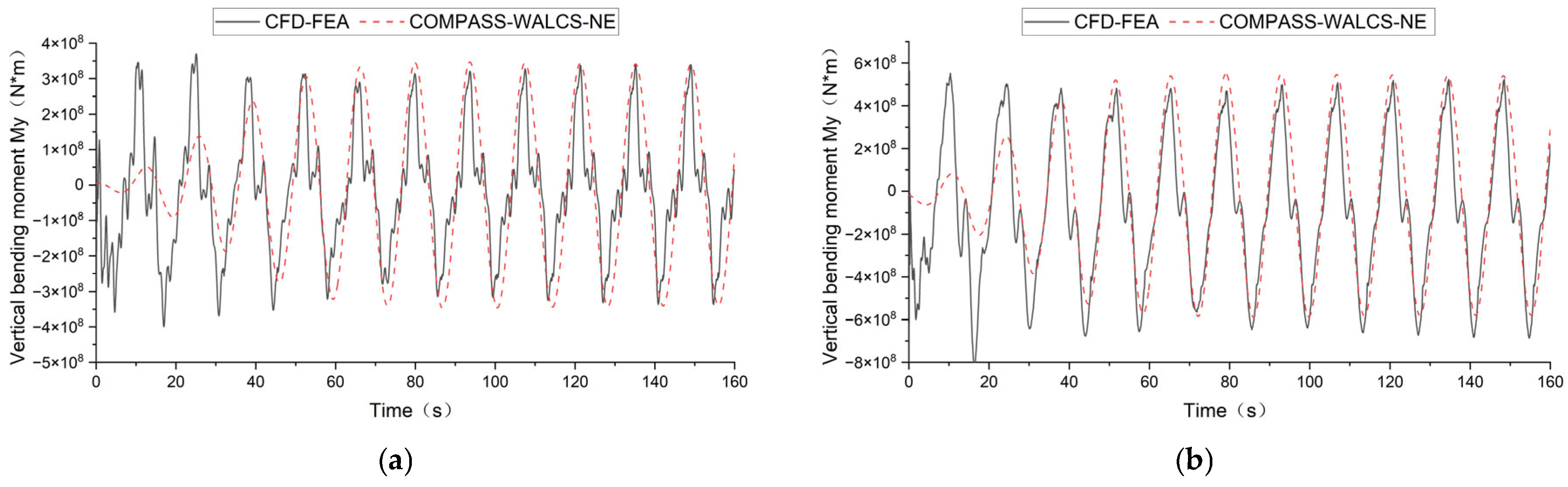
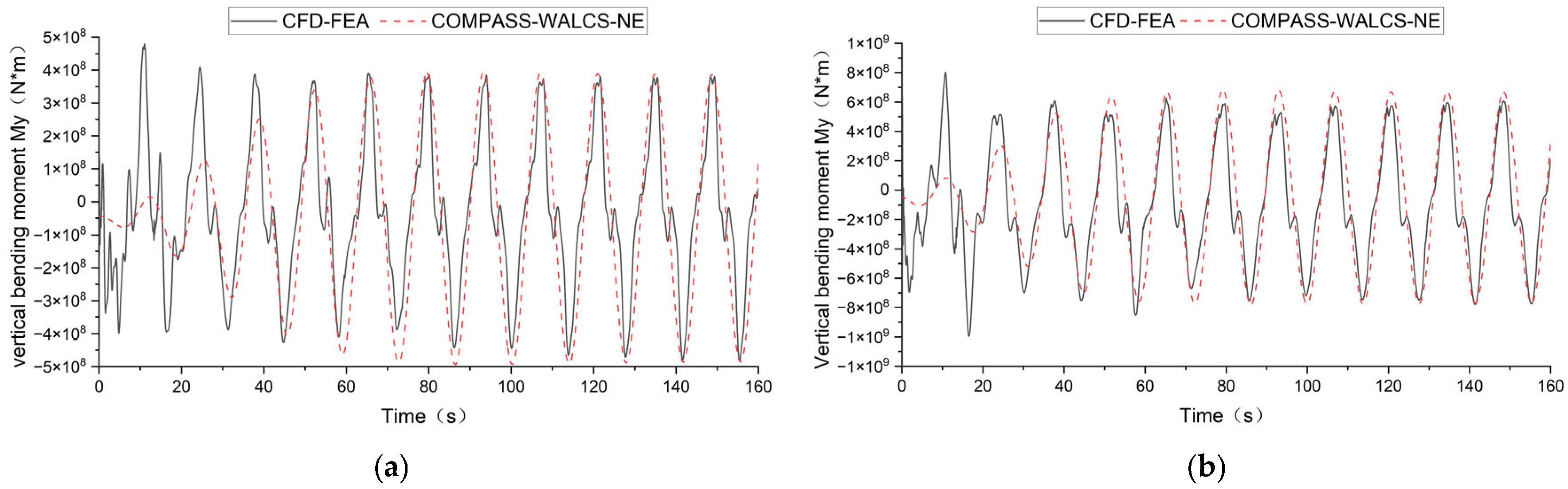
In this study, the hydrodynamic and structural responses of an unconventional large floating structure are simulated and analyzed using a CFD-FEA method. The results generated by the CFD-FEA method are compared with those generated by a rigid body linear frequency domain potential flow theory (WADAM) and by a three-dimensional potential flow nonlinear hydroelastic theory (COMPASS-WALCS-NE). Based on the analysis of the numerical results, the following concluding remarks can be drawn:

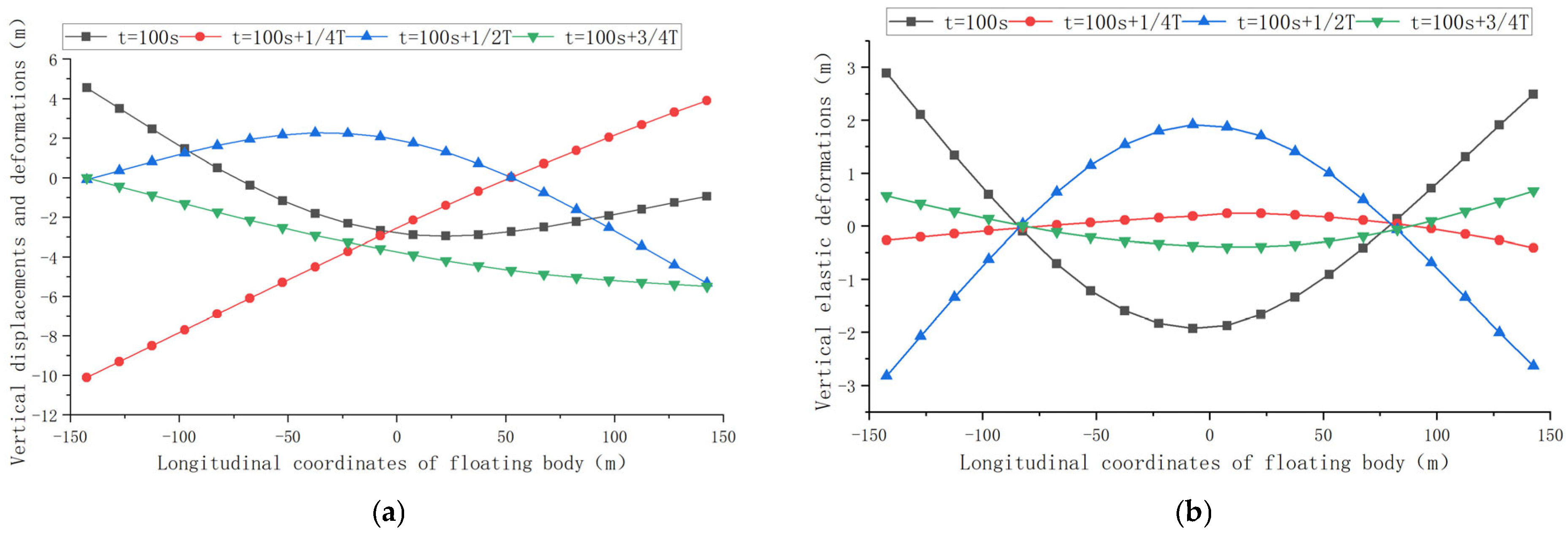
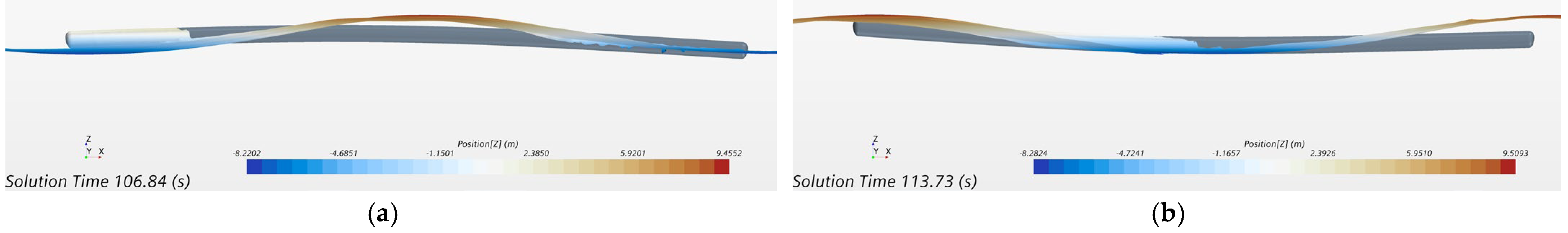
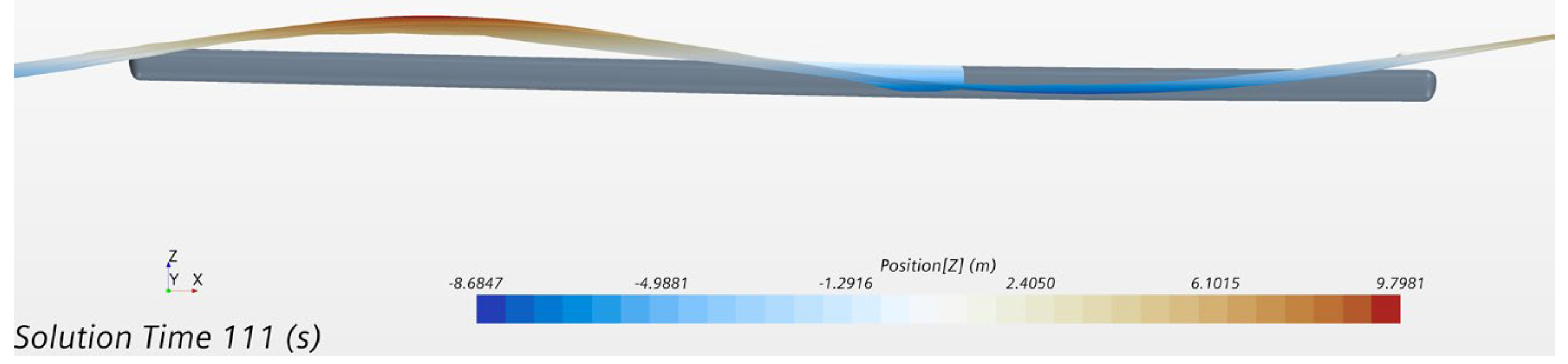
(1) The proposed CFD-FEA method can effectively exchange the information of the fluid domain and structure domain through the coupling interface, and a two-way coupling computation of the fluid domain and structure domain is realized. The numerical results of the elastic deformation of the floating body are reasonable.

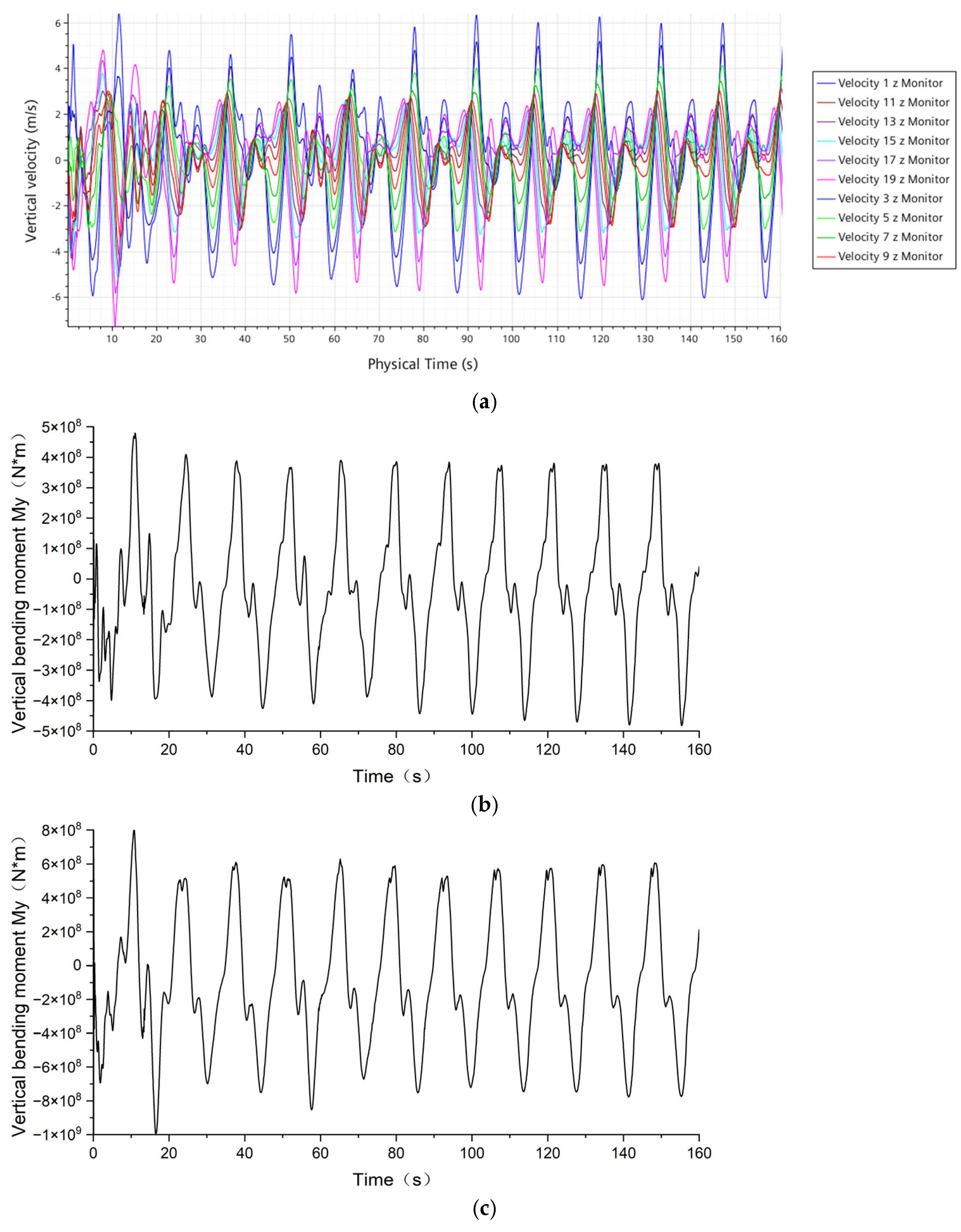
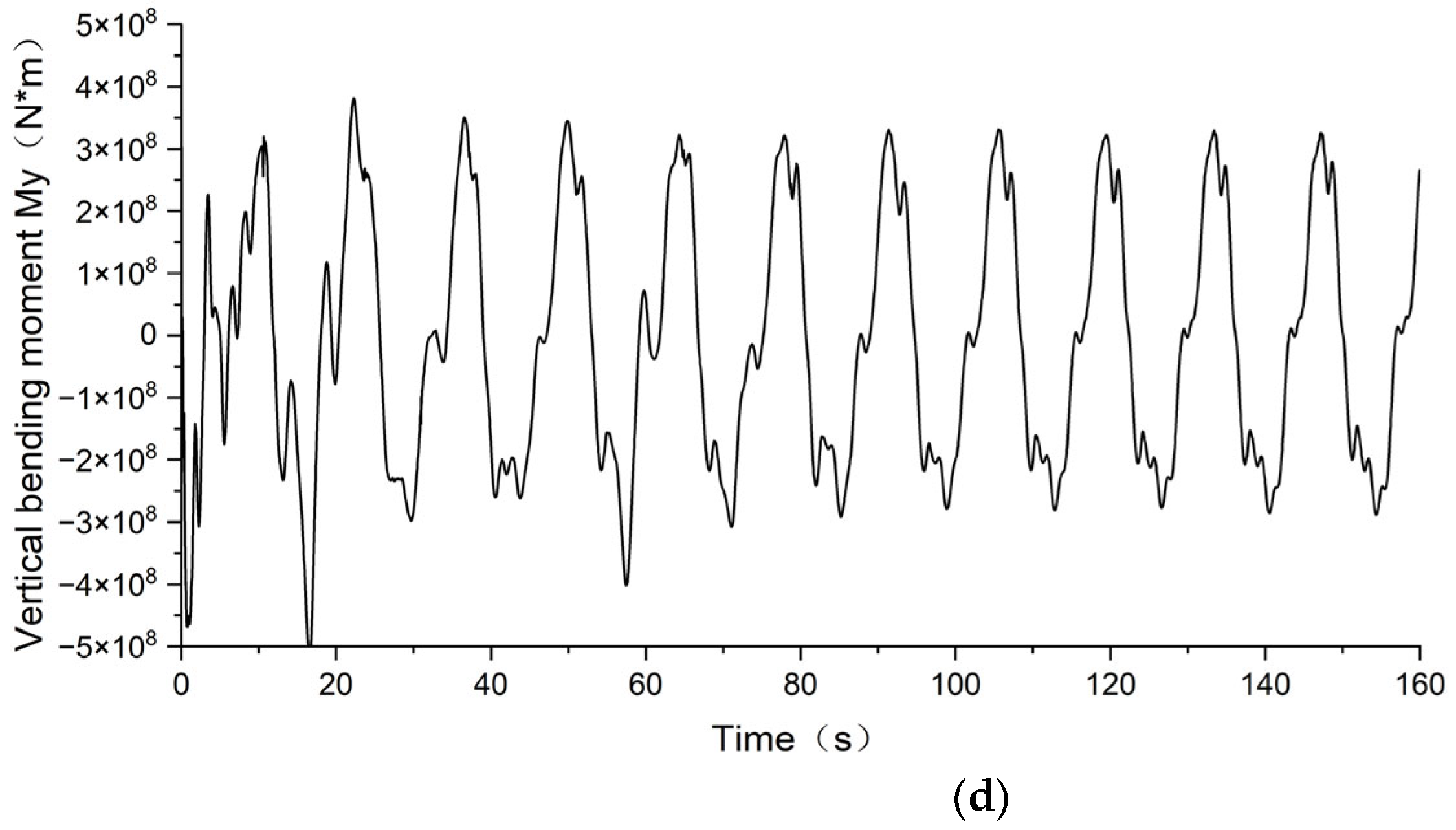
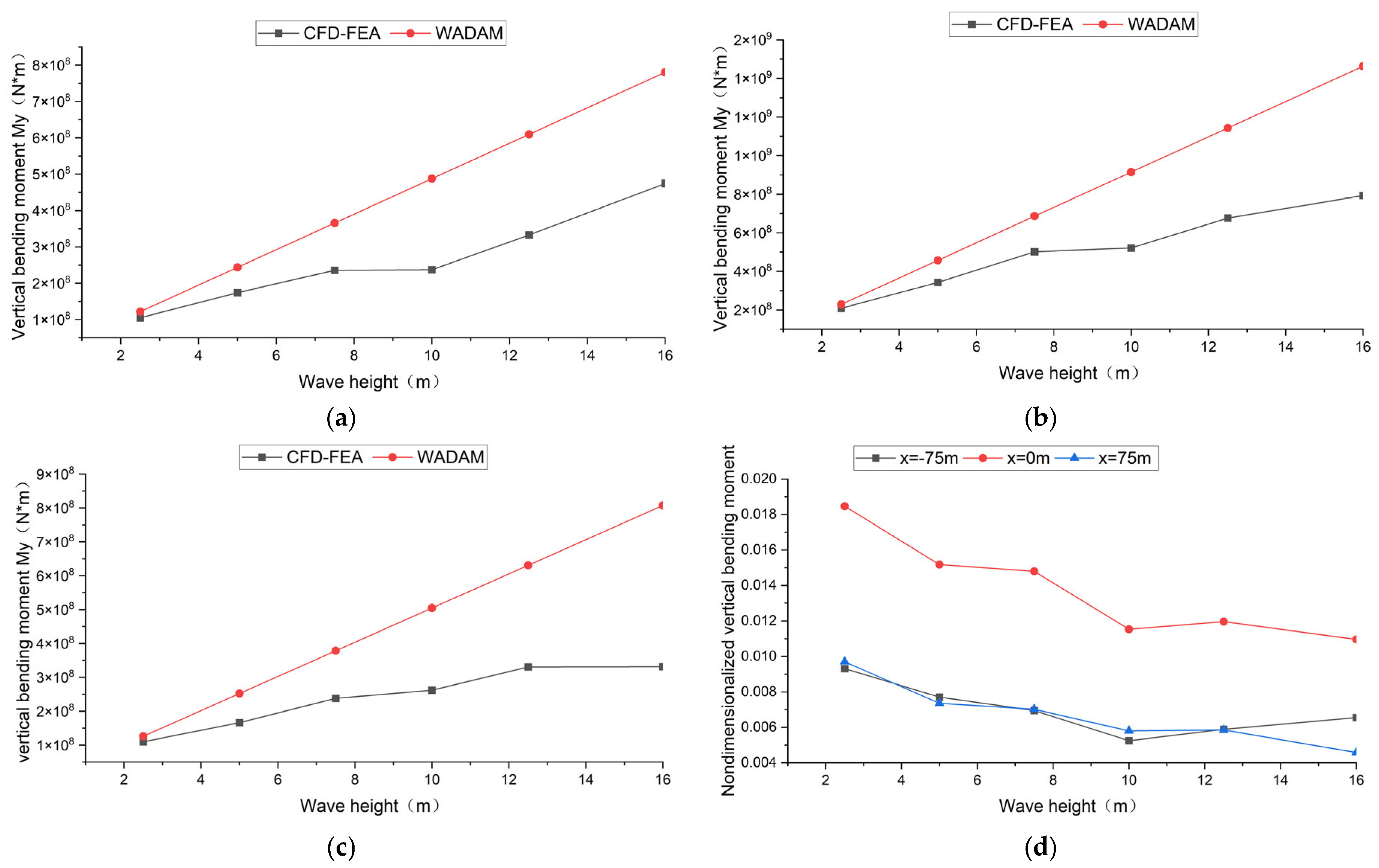
(2) In the case of large wave heights where wave overtopping occurs, the rate of an increase in the amplitude of the vertical bending moment $M_y$ obtained by the CFD-FEA method slowly decreases with the increase in the wave height. The amplitude of the vertical bending moment $M_y$ obtained by the CFD-FEA method is smaller than that by WADAM. Hydroelastic responses of elastic floating structures and nonlinear behaviors are observed in large wave heights, for which case COMPASS-WALCS-NE and the CFD-FEA method are recommended to solve such problems.

(3) For large wave heights, the peak values of the vertical bending moment $M_y$ obtained by the CFD-FEA method are in a good agreement with those by COMPASS-WALCS-NE, which shows that the CFD-FEA method is valid. Moreover, the CFD-FEA method can also capture complex phenomena, such as the details of the change in the vertical bending moment $M_y$, that the potential-flow-based methods cannot.

In this study, the CFD-FEA method for the hydroelastic response of large floating offshore structures is validated. Not only can the behavior of the hydroelastic responses of elastic floating structures be well estimated by the CFD-FEA method, but also the significant advantages of the CFD-FEA method over the traditional methods in capturing complex nonlinear behaviors are demonstrated.