
Evaluating Ice Load during Submarine Surfacing and Ice Breaking
by
 , , ,
, , ,
Liang Li
1,2,3,4,*,
Xiangbin Meng
5,
Alexander Bekker
6,
Oleg Makarov
6,
Wei Wang
1 and
Tao Zhang
7 
1
School of Civil Engineering, Harbin Institute of Technology, Harbin 150090, China
2
Hebei Key Laboratory of Earthquake Disaster Prevention and Risk Assessment, Sanhe 065201, China
3
Key Lab of Structures Dynamic Behavior and Control of the Ministry of Education, Harbin Institute of Technology, Harbin 150090, China
4
Key Lab of Smart Prevention and Mitigation of Civil Engineering Disasters of the Ministry of Industry and Information Technology, Harbin Institute of Technology, Harbin 150090, China
5
China Construction Engineering Company Limited (MACAU), Macau 999078, China
6
Department of Marine Arctic Technologies, Far Eastern Federal University, 690922 Vladivostok, Russia
7
China Ship Scientific Research Center, Wuxi 214082, China
*
Author to whom correspondence should be addressed.
J. Mar. Sci. Eng. 2023, 11(4), 736; https://doi.org/10.3390/jmse11040736
Submission received: 13 December 2022
/
Revised: 12 March 2023
/
Accepted: 22 March 2023
/
Published: 28 March 2023
(This article belongs to the Section Ocean Engineering)
Abstract
:At present, the calculation method of ice load on surface navigation ships has been very mature, but the calculation method of submarine ice load is very few. The reasonable evaluation of submarine ice load has become an urgent problem to be solved. In this paper, the mechanical characteristics of the submarine surfacing ice-breaking process are systematically analyzed. Based on the theory of plate and shell, the theoretical calculation models of ice-breaking resistance of the submarine command tower and hull are established, respectively, and the ice load calculation method of the command tower and the hull is obtained. Then, the submarine model SUBOFF is used to perform the numerical simulation of the submarine’s ice-breaking and surfacing process. The numerical result is compared with the ice-breaking resistance calculation model. The results show that the ice-breaking resistance calculation model proposed in this paper is consistent with the numerical simulation results, and the influence of parameters such as ice mechanical properties, the upper area of the command tower, and initial crack length on ice-breaking resistance is established. The calculation model in this paper can provide a theoretical reference for the optimization design of polar submarine structures.
1. Introduction
In recent years, researchers in various countries have increasingly focused on developing and conducting scientific research on Arctic shipping lanes. Global warming has made the Arctic regions more attractive for oil and gas exploitation [1,2]. Polar ships are essential equipment for polar exploration, shipping, and resource exploitation. Nowadays, polar icebreakers are commonly used to ensure smooth transportation in polar areas. Traditional icebreakers use above-water ice-breaking technology, where the weight of the hull or the bow’s collision crushes the ice [3,4,5,6]. Many countries worldwide are building or planning to build new-type polar ships to meet the needs of scientific research, waterway opening, escorting, and resource development [7]. The most advanced ice-breaking ship with the above-water method can break the ice layers with a maximum thickness of 3 m. However, during the winter of the Arctic, the average ice thickness is nearly 4 m, and the traditional ice-breaking methods of icebreakers became ineffective. Years ago, Russian scholars proposed the idea of a semi-submersible icebreaker, which uses the buoyancy of water to make the hull below the water float up and break through the ice layer. This type of icebreaker can break through solid ice layers with a thickness of more than 5 m [8]. Therefore, to maintain transportation in the polar region, it is necessary to develop upward-floating ice-breaking technology for the underwater hull. The study of the submarine-ice interaction can help to determine the ice-breaking resistance of underwater vessels and aid in the development of underwater ice-breaking technology.
The scientific study of the interaction between polar navigation vessels and ice has been a key research topic in the field of polar engineering. Ice-breaking resistance depends not only on the physical and mechanical properties of sea ice and the way the icebreaker breaks the ice but also on the damage pattern of the sea ice. To assess ice loads on ships, based on experimental data and the mechanical properties of sea ice, scholars have proposed many methods for calculating ice-breaking resistance (Lewis & Edwards [9]; Kotras et al. [10]; Lindqvist [11]; Keinonen et al. [12]; Riska et al. [13]; Spencer et al. [14]; Valanto [15]; Jeong et al. [16]; Li et al. [17]). The Lewis & Edwards and Lindqvist formulas are the more well-known formulas used to calculate ice-breaking resistance. Currently, the Keinonen and Riska formulas are also used. Both the Lewis & Edwards formula and the Lindqvist formula are based on analysis of model ship tests and real ship test data and each formula is accounting for different types of resistance. The Lewis & Edwards formula considers ice-breaking bending resistance, frictional resistance, ice-breaking resistance from dislodging and sinking broken ice, and resistance from hull collisions with broken ice, while the Lindqvist formula divides ice-breaking resistance into three components: ice-breaking bending resistance, breaking resistance and immersion resistance, each of which includes a velocity-dependent empirical factor. Riska’s formula and Keinonen’s formula are statistical formulas derived from ice-breaking test data on live ships in the Baltic Sea region. Riska’s formula relates ice-breaking resistance to ice thickness, speed, and hull geometry. Keinonen’s formula relates ice-breaking resistance to parameters such as hull geometry, hull environment, ice and snow thickness, ice bending strength, water salinity, and surface temperature. All four of these formulas, when considering the calculation of the bending resistance to ice-breaking subterm, regard the bending stress in the ice to reach the bending strength of the ice as the damage criterion, which in turn determines the bending resistance to ice-breaking. The above methods of assessing ice-breaking resistance are all based on surface vessels and do not take the vertical floating ice-breaking conditions of submerged vessels into account. However, an understanding of the development of ice-breaking calculation methods for surface vessels can be useful as a reference for the development of ice-breaking resistance calculation methods for submerged vessels.
The research on the calculation of the ice-breaking resistance of submerged vessels is still in its infancy, and relevant research at home and abroad is mainly based on experimental and numerical simulation methods. Scholars such as Kozin introduced the bending gravity wave generated by submarine motion under ice cover into the submarine ice-breaking process [18,19,20]. Kozin proposed a numerical model for analyzing the stress–strain state of the ice cover, which takes into account fractures of various widths caused by hydrodynamic loads due to submarine motion, and determined the relationship between deflection and stress amplitude in the ice layer and crack width when the submarine is surfacing at a speed less than the critical speed, where the inertial force is negligible compared to the elastic force. Based on the ice-breaking technology of bending gravity wave of submarine motion, scholars such as Kozin and Zemlyak have experimentally analyzed the influence of SV shape characteristics (submarine length and width) and bottom contour on ice-breaking efficiency and proposed that the ice-breaking ability to bend gravity wave can be evaluated by ice bending failure criterion [21,22].
Numerical simulation has emerged as a favorable approach for addressing the challenges presented by the testing conditions of ice-breaking studies, along with the development of numerical techniques. Numerical methods such as finite element (FEM), discrete element (DEM), smooth particle method (SPH), and proximate dynamics (PD) have been widely used to simulate the interaction between icebreakers with ice. Some scholars have started to use numerical methods to study the interaction mechanism between underwater ships and ice in the vertical direction. Ye and other scholars proposed an aerodynamics numerical model of submarine vertical floating and ice-breaking, then simulated the process of submarine lifting and ice-breaking and analyzed the time course changes in the law of ice load on submarine structure [23]. Wang et al. proposed a numerical simulation method of ice-water-structure coupling based on structured-arbitrary Lagrangian Eulerian fluid-solid coupling method and penalty function contact algorithm to address the problem of strong nonlinearity of structure-ice interaction by applying LS-DYNA finite element software to study the ice-breaking process of cylindrical vertical water exit [24]. Yue et al. obtained the main control parameters and similar laws affecting the dynamic load of underwater structures and their head stresses using dimensional analysis for the application context of underwater structures out of the water and breaking ice. Using LS-DYNA, numerical simulations were carried out for different initial velocities of underwater structures out of the water through different ice layers to obtain their dynamic load characteristics and mechanism of action [25].
The numerical analysis of ice load can explain the damage mechanism of sea ice, the characteristics of local ice pressure distribution, and the variation law of total ice force from different levels, which is an important way to study the interaction between sea ice and structures. However, the reliability of the computational model and the rationality of the computational parameters need to rely on an accurate ice mechanics model (physical model). Ice action models based on ice mechanics (physical models) are relatively few, but the works of Dempsey [26,27,28], and Maattanen and Hoikkanen [29], Rüdiger [30] can be mentioned. Sea ice is a multi-phase material consisting of pure ice, brine, air, and sometimes solid salts. Thus, a comprehensive mechanical model of ice would need to include linear and non-linear aspects of elasticity, visco-elasticity, visco-plasticity, and fracture [31]. under the influence of load, microcracks occur in the ice. The critical stress intensity factor (fracture toughness) is a criterion for when a crack will propagate, and it depends on the type of ice and the state of the ice. The size and number of cracks in the ice affect the ice load acting on the structure [32]. At present, scholars mainly use experimental methods and numerical simulation methods to study the icebreaking mechanism of the submarine and analyze the influence of submarine shape and ice conditions on icebreaking capacity, but there is no theoretical research on the evaluation method of ice resistance when submarine surfacing and breaking the ice. The calculation of the ice-breaking resistance of submarines in vertical floating has become an important problem for evaluating submarine navigation safety in ice areas, and it is also of great theoretical significance to the structural design of submarines moving in ice areas. Therefore, it is urgent to predict the ice-breaking resistance of submarines in vertical floating, which is also the purpose of this paper.
According to the study by Ye et al. [23], in the process of submarine surfacing and ice-breaking, the command tower first makes contact with the ice cover and then crushes through it, causing crushed ice to pile up around or on top of the command tower. After the command tower completely surfaced, as the hull continues to lift and break the ice, a large area of the ice layer is crushed and bent until the hull fully surfaces, and crushed ice piles up on the surface of the hull as well, as shown in Figure 1. The actual process of a submarine vertically lifting and breaking the ice is very complicated, making it difficult to calculate the ice resistance theoretically. According to the simplification of the submarine lifting and ice-breaking process, submarine ice-breaking resistance is divided into ice resistance for the command tower and ice resistance for the hull. To accurately predict the ice resistance, the mechanical characteristics of the submarine’s floating and ice-breaking processes are analyzed, and the theoretical calculation models of ice resistance to the submarine’s command tower and hull are established based on the theory of plate and shell mechanics. Subsequently, the ice loads on the submarine’s command tower and hull are calculated using the theoretical model and verified by the numerical simulation method. At last, the theoretical calculation model is used to investigate the influence of physical parameters of sea ice and submarine geometric dimensions on ice-breaking resistance.
In the following context, Section 2 states the establishment and derivation of a theoretical calculation model of ice load on a submarine hull and command tower. Section 3 shows the establishment and results of a numerical model of submarine floating and breaking ice. Section 4 introduces a comparison of the results of the theoretical model and numerical model, and a discussion of the influence of key parameters such as the thickness of sea ice, the upper area of the command tower, and initial crack length. Finally, Section 5 discusses the validity of the mechanical model in this paper, the relationship between key parameters and ice resistance of submarine lifting and breaking ice, and the theoretical support of the results of this paper for submarine design and navigation.
2. Theoretical Calculation Model of Ice-Breaking Resistance
2.1. Calculation Model of Ice-Breaking Resistance of Command Tower
The simplified model for the calculation of ice resistance of the submarine command tower is shown in Figure 2. The command tower first contacts the ice cover when the submarine surfaced. Assuming that the size of the ice sheet is much larger than the size of the command tower, it can also be said that the ice sheet can be approximately infinite in size in this model. According to Saint-Venant’s Principle, the stress of the non-contact part around the ice sheet is very small so that the ice layer can be simplified as a clamped rectangular plate subjected to a rectangle uniform load q in the central area of the plate (shaded part in Figure 2). The length and width of the plate are the areas of the load part . When a submarine is surfacing to break the ice, its speed of movement should be reduced as much as possible to maximize safety during the ice-breaking process. In this model, the effect of velocity is ignored from a hydrostatic point of view and the compression of the ice by the command tower is transferred to a distributed load. It is also assumed that sea ice is an isotropic elastic material. The type of ice rink in this article is level ice. According to the approximate theory of bending of plates subjected to out-of-plane loads, the thickness of the plate determines the deformation properties of the plate, the deflection of the ice plate is much less than the thickness of the ice layer, so the ice plate can be regarded as a thin plate with small deflection. Based on the theory of plate and shell mechanics, the deflection and stress of the plate under the bending are first determined, then the interaction force between the command tower and ice is calculated according to the ice bending failure criterion [33,34,35]. The interaction force is regarded as the ice load of the command tower. Rectangular ice plates are divided into load-affected areas () and non-load-affected areas (the parts above the line and beneath the line) according to the distribution of the uniform load. The deflection of the ice plates is divided into area and area below line (the deflection is equal to that of the part above the line ).
Following the force analysis diagram of the ice plate in Figure 2, the differential equation for the ice plate deflection surface under the distributed load q can be formulated.
M. Levy’s method is used to determine the deflection of the clamped rectangular plate subjected to uniform load [36]. The deflection of the ice plate in area is equivalent to the sum of the deflection and , where is the deflection of the plate parallel to the x axis under uniform load and is the deflection that ensures meets all boundary conditions of the ice plate. Therefore, the deflection of the ice plate in the area is
where
According to Equations (3) and (4), the deflection of ice plate in area can be determined as follows
where
From Equations (3)–(7), D is the flexural rigidity of the ice plate, h is the thickness of the ice plate and is Poisson’s ratio of the ice plate.
For the plate bearing no load at the lower part of the line, refer to M. Levy’s method to set the deflection of the ice plate in this area as
According to the internal force, geometric continuity conditions, and the boundary conditions of the plate, six undetermined constants , , , , and , in formulas Equations (5) and (8) can be determined.
Geometric continuity condition: The geometric requirements along the line, when y is equal to , the following two equations are obtained.
Internal force continuity condition: The bending moment and shear force along line are continuous, according to the continuous condition, when y is equal to , the following equation can be obtained:
Boundary conditions: The ice layer is regarded as clamped rectangular plate, when y is equal to the , the following two equations can be obtained:
The six constants can be solved by combining Equations (10), (11), (13), (14), (16) and (17). The expressions for the constants to be solved are as follows.
The specific expressions of and are:
The deflection of a thin plate subjected to a uniform load at its center is obtained by substituting the six constants to be determined into Equations (5) and (8), respectively. The relationship between the deflection and the bending moment and shear force of the ice plate is as follows:
The stress expression of any microelement in the ice plate is as follows:
Substituting the obtained , , , , , into Equations (32)–(38). It can be seen that the stresses on the ice plate microelements are all functions of variables q and z, z is the coordinate axis in the thickness direction of the ice plate, and the middle plane of the ice plate is where z is equal to zero. The stresses on the ice plate will change as uniform load q fluctuates, and the stresses vary with the thicknesses (different values of z) of the ice plate.
According to the stress state of the ice plate from Equation (32) to Equation (38), the stress level of the ice plate is directly related to the uniformly distributed load. Existing failure criteria for the bearing capacity of floating ice sheets predict the load for the occurrence of the first radial crack or a circumferential crack when the maximum stress obtained from an elastic analysis in the ice equals the bending strength. According to Newton’s third law, the ice load on the command tower should be the same as the force exerted by the command tower on the ice plate. Therefore, the key to the problem is to find out the range of the uniform load.
The characteristic equation for the stress state of the ice plate micro-element is as follows:
In this equation: —first invariant of the stress tensor;
—second invariant of the stress tensor;
—third invariant of the stress tensor.
The failure of ice shows brittle fracture characteristics. In this paper, the classical maximum normal stress criterion is used to verdict the failure of ice plates. Three principal stresses , and can be obtained from the characteristic equation of stress state, and they are all one-dimensional cubic functions of the uniform load q. Using the maximum normal stress criterion, the uniform load q can be obtained. The product of the uniform load q and the upper area of the command tower is the ice resistance of the command tower when the submarine surfaces and breaks the ice.
2.2. Calculation Model of Ice Resistance of Submarine Hull
After the command tower breaks through the ice, the submarine continues lifting and the hull contacts with the ice layer and starts to break the ice. The ice rink can be approximately infinite in size. Since the length of the crack generated by the command tower on the ice layer is relatively small compared with the ice plate, the ice layer is regarded as a plate with the initial crack when calculating the ice resistance of the hull. The effect of the hull on the ice layer is simplified as distributed p acting on the plate [17,37]. The initial crack length is v, the width and length of the plate are a and b, and the thickness is h. In this model, a finite-size rectangular plate is used instead of an infinite-size ice plate, and the four sides of the rectangular plate are bounded by fixed boundary conditions. The theoretical model for calculation is shown in Figure 3.
According to Figure 3, stress concentration occurs at point A. From the literature [38], a rectangular plate of equal thickness with one crack, under transversely distributed load (vertical action), we have the expression of stress intensity factor :
where ; ; v is the initial crack length of the ice plate; is Poisson’s ratio of sea ice; h is the thickness of the ice plate; p is distributed load on the ice plate; considering the actual situation of submarine floating and ice-breaking process, the contact area between the hull and the ice plate increases gradually with the floating process, so the distributed load reduction factor is introduced here. Ji Shunying et al. from the Dalian University of Technology gave the expression of the fracture toughness of ice based on experimental results [39].
where T is the temperature of sea ice.
Ice is considered as a plate with initial cracks when calculating hull ice break-up, when ice is subjected to lateral loads, according to the crack instability criterion, when the stress intensity factor reaches the fracture toughness of the ice. Cracking of the ice sheet expands and damage to the ice sheet occurs. Therefore, the uniform load p can be obtained once fracture toughness is determined. The maximum cross-sectional area in the horizontal direction of the submarine hull times the uniform load p is equal to the ice resistance of the submarine hull.
3. Numerical Simulation
3.1. Establishment of Numerical Model
Numerical simulation is widely used in the research of interaction between icebreakers and ice [40,41,42,43]. To verify the theoretical calculation model of the submarine’s floating ice resistance, numerical simulations are performed using the finite element code LS-DYNA to simulate the process of submarine lifting and ice-breaking. The US DARPA submarine model SUBOFF was selected as the research object [44]. The submarine has a total length of 104.544 m and its hull is divided into three parts: the forebody, the parallel middle body, and the afterbody. The command tower is located 22.176 m from the front end of the hull. In addition, the SUBOFF submarine model has four trail fins around the tail. Since this paper mainly studies the ice load on the command tower and the hull in the process of floating and ice-breaking and the four trail fins are very small compared with the command tower, the four fins are neglected in the simulations [45]. The ice rink in the cold zone can be regarded as infinite. In the numerical models, the actual ice rink will be replaced by a fixed ice plate (150 m × 36 m × 0.9 m). Both the submarine model and the ice rink model are built with SOLID164 solid elements.
Since the ice resistance of the submarine in the process of floating is the focal point of this study, only the shape of the submarine is considered and the material model of the submarine is set as a rigid body [46,47]. Sea ice is regarded as an elastic brittle material and the material model parameters defining the ice plate are shown in Table 1 [23,34]. Sea ice is modeled using an elastic-brittle model, and the failure of sea ice materials uses a strength criterion. When the stress reaches the permissible strength, damage to the sea ice occurs and crack development begins.
In the natural environment, the ice rinks float on the surface of the water. In the numerical simulation process, rigid planes are used to support the ice plates to simulate the actual fluid buoyancy effect [6,48,49]. In the numerical simulations, the submarine is set to have an initial constant speed to simulate the buoyancy effect on the submarine. In addition, it is necessary to consider that the submarine floats at a very low speed, which is mainly because the submarine will not hit the ice at a very high speed to ensure its safety. When a submarine is surfacing to break the ice, its speed of movement should be reduced as much as reasonably possible to maximize safety during the ice-breaking process. Furthermore, we can see that when the submarine is moving at a very small speed, the effect of speed on the ice load is already very small. The specific speed value is 0.005 m/s. The submarine will first slowly contact the ice with the command tower and float slowly, and the sea ice will break because of shear and bending force. The contact type between the submarine and ice plate is surface-to-surface. The finite element model of the submarine and the ice plate is shown in Figure 4.
In numerical simulations, the appropriate element size can not only ensure the accuracy of the calculation results but also improve the calculation efficiency. In the numerical model, the mesh division of the submarine in the numerical model is kept regular and uniform. The ice plate is meshed with three different sizes to investigate the effect of meshing size: 0.2 m × 0.2 m × 0.225 m, 0.2 m × 0.2 m × 0.3 m, and 0.3 m × 0.3 m × 0.3 m. Through calculation and comparison, it was observed that compared with the grid size of 0.2 m × 0.2 m × 0.225 m, the average difference in calculated ice loads is about 4%. so the grid size of 0.3 m × 0.3 m × 0.3 m × 0.3 m meets the accuracy requirement. In addition, when the grid size is 0.3 m × 0.3 m × 0.3 m, the calculation time of the model is 18 h, which is 57% less than the 42 h when the grid size is 0.2 m × 0.2 m × 0.3 m, and 65% less than when the grid size is 0.2 m × 0.2 m × 0.225 m.Therefore, the size of the ice plate selection unit is 0.3 m × 0.3 m × 0.3 m. After meshing, the whole finite element model has 201,311 elements and 568,160 nodes.
3.2. Numerical Simulation Results
Figure 5 shows the numerical simulation process of a submarine surfacing and ice-breaking in this study. Figure 5a,b show the process of ice-breaking of the command tower. The command tower first contacts the ice cover and starts to break the ice. As the submarine slowly floats up, cracks appeared on the ice plate. Subsequently, the submarine continues to float upward and the command tower broke out of the ice. In the meantime, some of the sea ice piles up on top of the command tower and some damaged sea ice piles up around the command tower. Figure 5c,d show the process of ice-breaking of the hull. After the command tower broke out of the ice layer, the hull continues to float upward and the ice layer first produced huge cracks, and then bent and damaged, which lead to the accumulation of sea ice on the surface of the hull. The numerically simulated process of submarine floating and ice-breaking is in good agreement with the actual situation, which verifies the effectiveness of the numerical model.
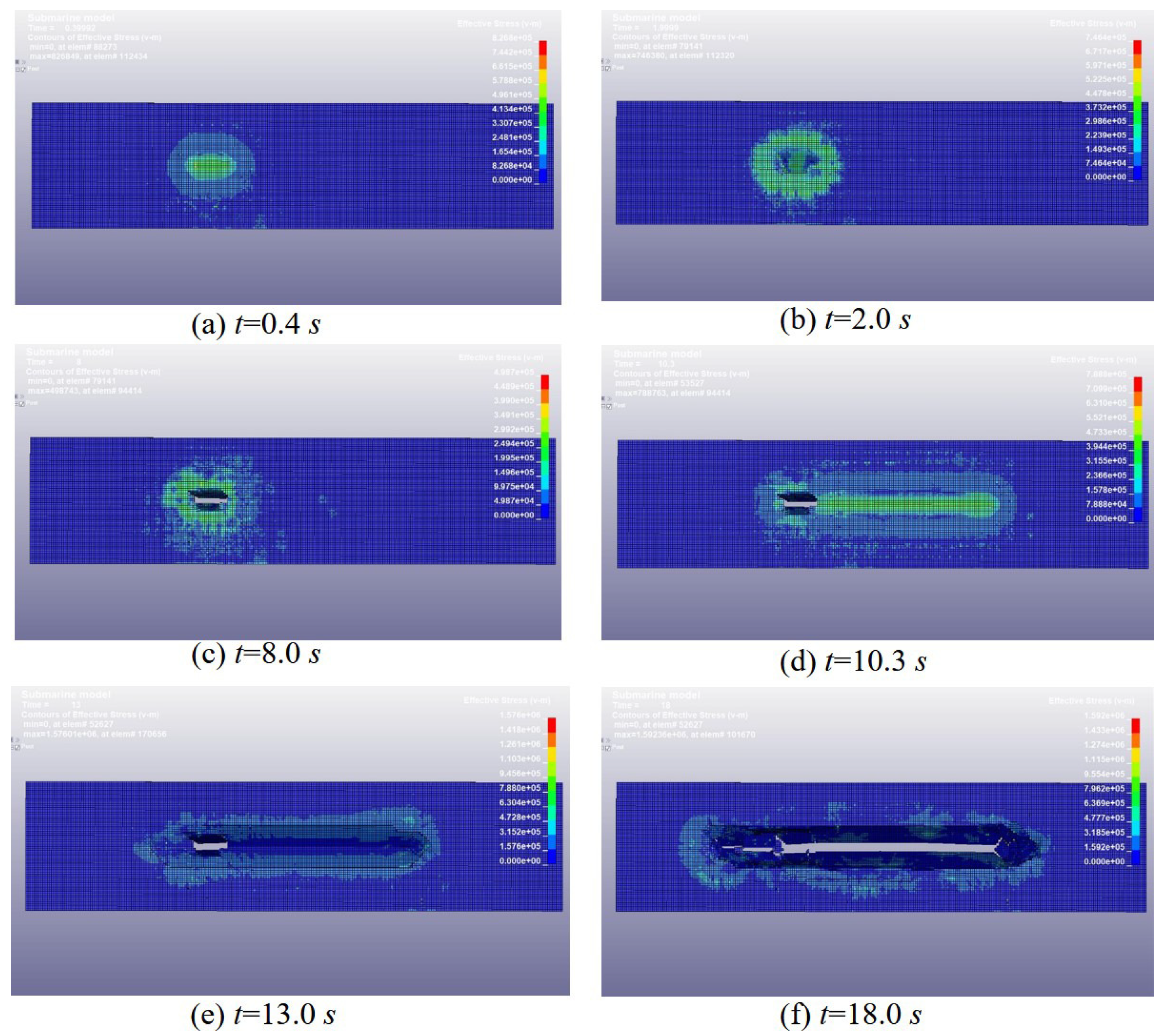
Figure 6 shows a distribution map of the von Mises equivalent force in the ice sheet at different moments when the submarine is out of the water and crossing the ice. When s, after the submarine has moved vertically upwards and contact between the command tower and the bottom of the ice occurs, a similar elliptical stress distribution occurs in the ice above the command tower, with the central region being the stress concentration area as shown in Figure 6a. As the submarine command tower continued its upward movement, the stresses in the central region of the ellipse increased, and when the stresses reached the strength limit of the sea ice material, the ice sheet cracked and broke down, and stress unloading occurred in the central region, after which the command tower had crossed the ice and broken ice appeared on it, as shown in Figure 6b,c. After the submarine command tower crossed the ice, the hull of the submarine also came into contact with the ice and a striped area of stress distribution appeared in the ice of the boat, as shown in Figure 6d. As the submarine’s hull continued to move vertically upwards, the ice was squeezed by the hull and the ice stress reached the strength limit of the sea ice material when an elliptical ring of cracks appeared around the area of strip stress, as shown in Figure 6e. As the submarine continued to float vertically, a large number of cracks appeared in the ice on the upper part of the hull and the submarine broke through the ice, causing the upper ice to fail and a crack to form in the middle of the ice sheet, creating an area of fast accumulation of broken ice in the upper area of the submarine, as shown in Figure 6f.
3.3. Comparison of Theoretical Model and Numerical Simulation Results
In the process of submarine floating and ice-breaking, the submarine needs to float slowly. After contact with the ice layer, compressed air will discharge the water in the ballast tank bit by bit to increase buoyancy and decrease its gravity until it cracks the ice. This process is called “static loading”. During the simulations, the floating speed is kept at 0.005 m/s to simulate the real floating process. According to the numerical simulation results, the ice loads of the submarine command tower and the hull are 247 kN and 1290 kN, respectively. The theoretical model proposed in this paper is applied to calculate the ice load, and the result shows that the ice loads of the submarine command tower and the hull are 231 kN and 1117 kN, respectively. By comparison, it is found that the difference between the numerical and theoretical results of ice loads is 6% in the command tower and 13% in the hull. In the numerical simulation, only the gravity of the ice plate is considered, and the change of buoyancy of the ice plate is not considered, which will lead to a slightly larger numerical simulation result. In general, the theoretical calculation model of submarine floating and ice-breaking resistance is feasible.
4. Results and Discussion
4.1. The Influence of the Upper Area of the Control Tower
The influence of the upper area of the command tower on the ice load is analyzed in this section. Because in the theoretical calculation part, the effect of the command tower on the ice plate is considered as a rectangular uniform load, with the load area of , the ratio of is kept unchanged, and the size of u and v is changed for calculation.
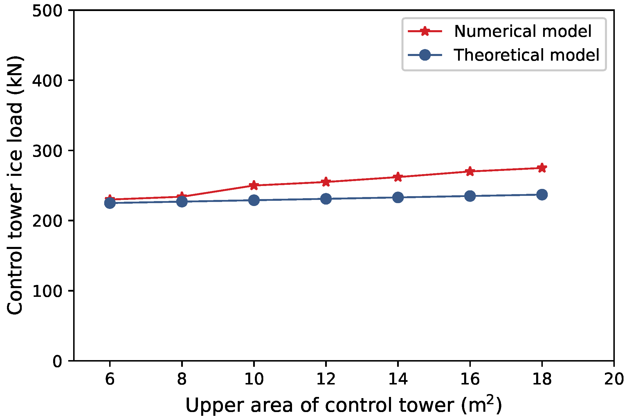
Figure 7 shows the relationship curve between the ice load of the command tower and its upper area. According to Figure 7, the area of the upper part of the command tower has increased by 2 times from 6.0 m to 18 m, and the ice load calculated by the theoretical model has increased by 0.04 times from 225 kN to 234.5 kN. The ice load calculated by the numerical model increases from 230 kN to 275 kN, an increase of 0.2 times. With the increase of the upper area of the command tower, the ice load of the command tower increases slowly. When designing the submarine structure, the upper area of the command tower should also be reduced as much as possible under the condition that the service conditions can be met, to ensure the safety of the submarine structure when the submarine floats up and breaks the ice.
4.2. The Influence of Initial Crack Length on Submarine Ice-Breaking Resistance
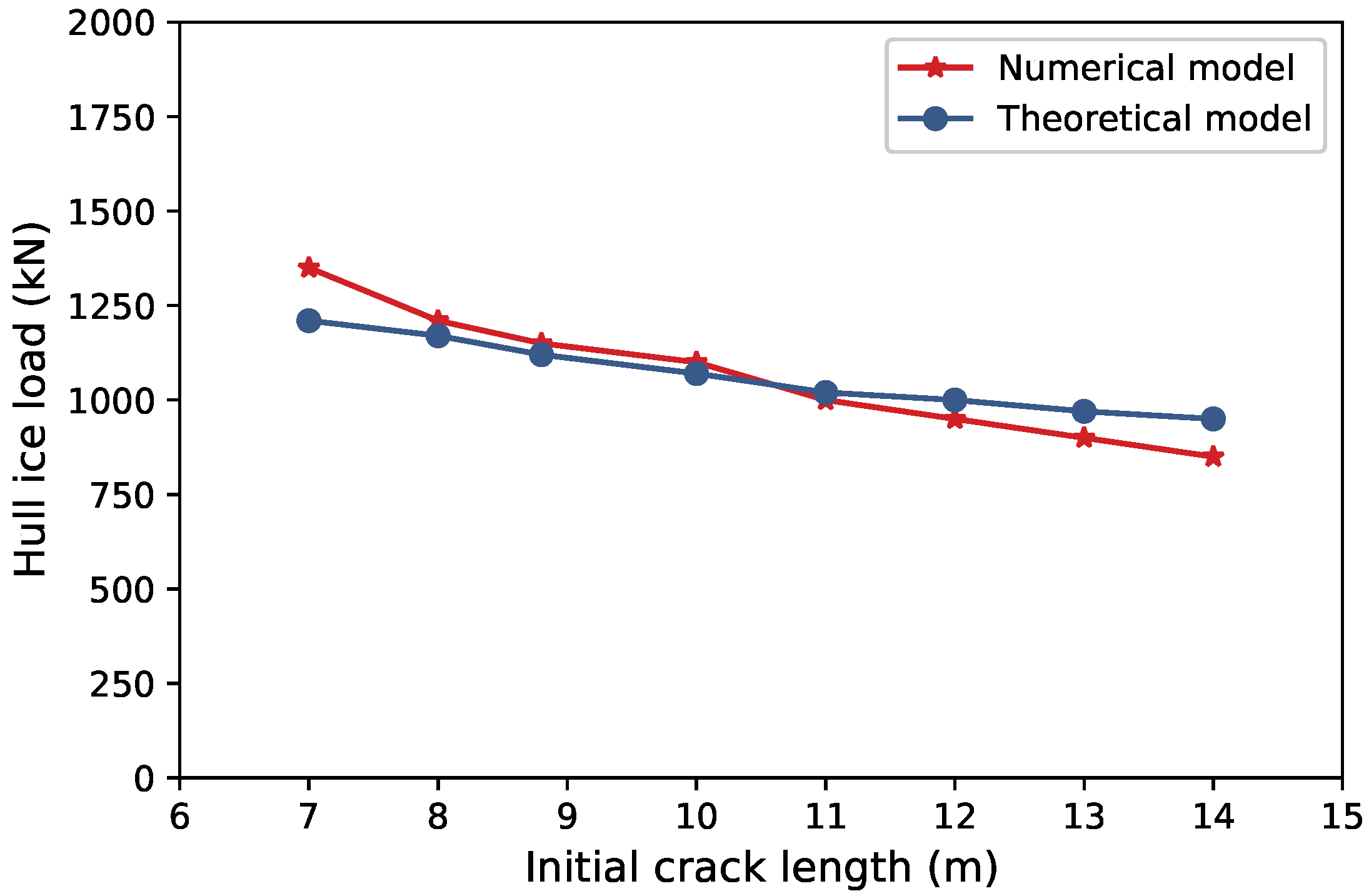
When calculating the ice load on the hull, the flat ice is regarded as a flat plate with initial cracks, and the influence of the crack length of the ice plate on the ice load on the hull needs to be investigated. Figure 8 shows the relationship curve between crack length and ice load on the hull. According to Figure 8, the ice load on the hull calculated by the theoretical model and the numerical model have similar trends, and the determined ice load decreases with the increase of crack length. This can be explained by the definition of stress intensity factor, which is a physical quantity reflecting the strength of elastic stress at the crack tip: with the increase of the initial crack length, the stress intensity factor increases, which means that the more concentrated the stress at point A of the crack tip, the smaller the force required to destroy the structure.
4.3. The Influence of Ice Thickness on Submarine Ice-Breaking Resistance
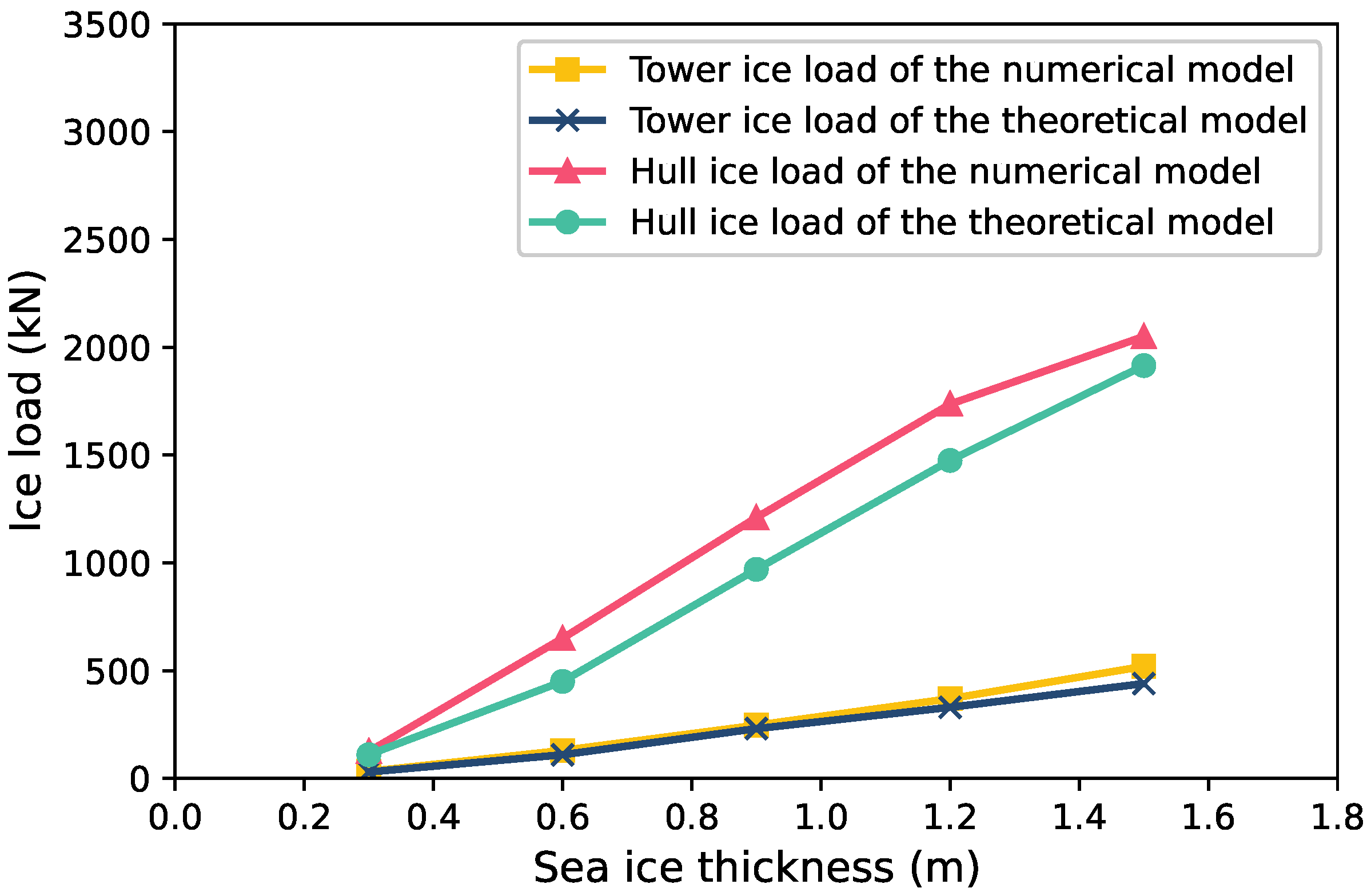
The thickness of sea ice has a direct impact on the navigation safety and ice-breaking performance of ships. Generally speaking, the ice load acting on the ship will increase with the increase in ice thickness. Figure 9 shows the influence curve of sea ice thickness on submarine ice load. The sea ice thickness varies from 0.3 m to 1.5 m, keeping other parameters of the submarine and ice layer unchanged. It can be seen from Figure 9 that with the increase in sea ice thickness, the ice load of the command tower and the ice load of the hull are also increasing. When the sea ice thickness increases from 0.3 m to 1.5 m, the ice load of the command tower increases by 4 times. The ice load of the command tower calculated by the theoretical model increases from 30 kN to 440 kN. The ice load of the command tower calculated by the numerical model increases from 33 kN to 520 kN. The ice load of the command tower increases by about 14 times. When the sea ice thickness increases from 0.3 m to 1.5 m, the ice load on the hull calculated by the theoretical model increases from 110 kN to 1915 kN, and the ice load on the hull calculated by the numerical model increases from 125 kN to 2050 kN, and the ice load on the hull increases by about 16 times. With the increase of sea ice thickness, the increase of ice load on the hull is faster than that on the command tower. As can be seen from Figure 9, the thickness of sea ice has a great impact on the ice load generated by submarine floating and ice-breaking. When a submarine floating and ice-breaking, it should be carried out at the thinner ice layer to ensure the structural safety of the submarine.
4.4. The Influence of Ice Bending Strength
In the ice load theoretical model of the command tower, bending strength is one of the mechanical performance indexes of sea ice, and is the key index to judge the sea ice damage when the submarine command tower breaks the ice. Figure 10 shows the relationship curve between the ice load and sea ice bending strength of the command tower. It can be seen from Figure 10 that with the increase of sea ice bending strength, the ice load on the command tower is also increasing. When the bending strength of sea ice increases from 0.36 MPa to 1.5 MPa, it increases by about 3 times. The ice load of the command tower calculated by the theoretical model increases by about 3 times from 231 kN to 900 kN. The ice load of the command tower calculated by the numerical model increases by about 3 times from 247 kN to 950 kN. From the results, it can be found that the ice load on the command tower is linearly related to the bending strength of sea ice, and the calculation results of the theoretical model and the numerical model are similar.
4.5. The Influence of Ice Elastic Modulus
Elastic modulus is the most important mechanical parameter in the elastic analysis of materials. According to the existing experimental data on the mechanical properties of sea ice, the elastic modulus of sea ice varies from 1 GPa to 4 GPa. Figure 11 shows the relationship curve between submarine ice load and sea ice elastic modulus. According to Figure 11, with the increase of the elastic modulus of sea ice, the ice load on the command tower and the ice load on the hull increase slowly, and the growth rate of the ice load on the hull is slightly greater than the growth rate of the command tower.
4.6. The Influence of Ice Friction Coefficient
When a submarine floats up to break the ice, both the hull and the command tower come into contact with the sea ice, creating frictional resistance, which in turn affects the resistance to breaking the ice. Whether the friction coefficient between submarine and sea ice affects the ice load needs to be analyzed. The friction coefficient is easily affected by the roughness of the material surface. The shells of submarines are generally made of high-strength steel. In this paper, the friction coefficient between ice and the submarine’s outer surface varies from 0.1 to 0.5 (Coefficient of friction between ice and steel). Figure 12 shows the relationship curve between submarine ice load (Command tower and hull) and sea ice friction coefficient. It can be seen from Figure 12. that with the increase of the friction coefficient between ice and the submarine, the ice load of the command tower and the ice load of the hull increase very slowly, and the increase of the ice load is about 2%.
5. Conclusions
Based on the mechanics of plate and shell, the mechanical models of submarine lifting and breaking ice by command tower and hull are established systematically in this paper. In addition, the finite element numerical model of submarine floating and ice-breaking is established to simulate the ice-breaking process. According to the results, several conclusions are made: (1) according to the submarine floating and ice-breaking mechanical model and numerical simulation, the ice-breaking load of the command tower and the hull are calculated, respectively, and the relative errors are 6% and 13%. The mechanical model established in this paper is able to evaluate the ice-breaking load of submarine floating and ice-breaking; (2) it is found that the ice thickness and the ice elastic modulus are directly proportional to the submarine ice load, while the initial crack length of the ice plate is inversely proportional to the hull ice load. It reveals the influence of the parameters such as the ice thickness, the upper area of the command tower and the initial crack length of the ice plate on the submarine lifting ice load.
Based on the research results of this paper, it can provide technical support for the study of submarine navigation in polar regions, and also provide theoretical guidance for the engineering design of submarine hull structures. However, in order to calculate the lifting ice load of a submarine more accurately, it is necessary to carry out a systematic theoretical analysis of the relationship between the gravity of the ice plate and the buoyancy of water.
Author Contributions
Conception, L.L., A.B. and W.W.; Methodology, L.L., X.M. and O.M.; Investigation, L.L., X.M. and T.Z.; Validation, L.L., X.M. and A.B.; Writing—original draft preparation, L.L.; Writing—review and editing, L.L. and A.B. Project administration, L.L. All authors have read and agreed to the published version of the manuscript.
Funding
This research was supported by Grant from the National Natural Science Foundation of China (Grant No. 51609054), and Hebei Key Laboratory of Earthquake Disaster Prevention and Risk Assessment (Grant No. FZ213103), and the Fundamental Research Funds for the Central Universities (Grant No. HIT. NSRIF. 2017065).
Institutional Review Board Statement
Not applicable.
Informed Consent Statement
Not applicable.
Data Availability Statement
Not applicable.
Conflicts of Interest
The authors declare no conflict of interest.
References
- Zhang, J.; Wu, Q.; Zhao, X. Analysis of Polar Class Ship Development. Ship Eng. 2016, 11, 1–5. [Google Scholar]
- Liu, R.W.; Xue, Y.Z.; Lu, X.K.; Cheng, W.X. Simulation of ship navigation in ice rubble based on peridynamics. Ocean. Eng. 2018, 148, 286–298. [Google Scholar] [CrossRef]
- Suyuthi, A.; Leira, B.J.; Riska, K. A generalized probabilistic model of ice load peaks on ship hulls in broken-ice fields. Cold Reg. Sci. Technol. 2014, 97, 7–20. [Google Scholar] [CrossRef]
- Lee, J.M.; Lee, C.J.; Kim, Y.S.; Choi, G.G.; Lew, J.M. Determination of global ice loads on the ship using the measured full-scale motion data. Int. J. Nav. Archit. Ocean. 2016, 8, 301–311. [Google Scholar] [CrossRef] [Green Version]
- Di, S.; Ji, S.; Xue, Y. Analysis of ship navigation in level ice-covered regions with discrete element method. Ocean. Eng. 2017, 35, 59–69. [Google Scholar]
- Lubbad, R.; Loset, S. A numerical model for real-time simulation of ship–ice interaction. Cold Reg. Sci. Technol. 2011, 65, 111–127. [Google Scholar] [CrossRef] [Green Version]
- Huang, Y.; Guan, P.; Mu, Y.U. Study of the Sailing’s Moving Responses of An Icebreaker in Ice. Math. Pract. Theory 2015, 45, 149–160. [Google Scholar]
- Liang, Y.; Ji, H.; Zhao, Q.; Wu, H.; Liu, Z. Technical progress of Russian submarine ice navigation tests. Mar. Equip./Mater. Mark. 2021, 29, 1–6. [Google Scholar]
- Lewis, J.; Edwards, R. Methods for predicting icebreaking and ice resistance characteristics of icebreakers. SNAME Trans. 1970, 78, 213–249. [Google Scholar]
- Kotras, T.; Baird, A.; Naegle, J. Predicting ship performance in level ice. Trans. Soc. Nav. Archit. Mar. Eng. SNAME 1983, 91, 329–349. [Google Scholar]
- Lindqvist, G. A straightforward method for calculation of ice resistance of ships. In Proceedings of the International Conference on Port and Ocean Engineering under Arctic Conditions (POAC), Lulea, Sweden, 12–16 June 1989; pp. 722–735. [Google Scholar]
- Keinonen, A.; Robbins, I. Icebreaker Characteristics Synthesis; Report for the Transportation Development Centre; Report (TP12812E); Transport Canada: Ottawa, ON, Canada, 1996. [Google Scholar]
- Riska, K.; Wilhelmson, M.; Englund, K.; Leiviska, T. Performance of merchant vessels in the Baltic; Report 52; Helsinki University of Technology: Helsinki, Finland, 1997. [Google Scholar]
- Spencer, D.; Jones, S.J. Model-Scale/Full-Scale Correlation in Open Water and Ice for Canadian Coast Guard “R-Class” Icebreakers. J. Ship Res. 2001, 45, 249–261. [Google Scholar] [CrossRef]
- Valanto, P. The resistance of ships in level ice. SNAME Trans. 2001, 109, 53–83. [Google Scholar]
- Jeong, S.; Lee, C.; Cho, S. Ice Resistance Prediction for Standard Icebreaker Model Ship. In Proceedings of the Twentieth International Offshore and Polar Engineering Conference, Beijing, China, 20–25 June 2010; pp. 1300–1304. [Google Scholar]
- Li, L.; Gao, Q.; Bekker, A.; Dai, H. Formulation of Ice Resistance in Level Ice Using Double-Plates Superposition. J. Mar. Sci. Eng. 2020, 8, 870. [Google Scholar] [CrossRef]
- Kozin, V.M.; Chizhumov, S.D.; Zemlyak, V.L. Influence of ice conditions on the effectiveness of the resonant method of breaking ice cover by submarines. J. Appl. Mech. Technol. Phys. 2010, 51, 398–404. [Google Scholar] [CrossRef]
- Pogorelova, A.; Zemlyak, V.; Kozin, V. Moving of a submarine under an ice cover in fluid of finite depth. J. Hydrodyn. 2019, 31, 562–569. [Google Scholar] [CrossRef]
- Sturova, I. The motion of a submerged sphere in a liquid under an ice sheet. J. Appl. Math. Mech. 2012, 76, 293–301. [Google Scholar] [CrossRef]
- Zemlyak, V.; Pogorelova, A.; Kozin, V. Influence of peculiarities of the form of a submarine vessel on the efficiency of breaking ice cover. In Proceedings of the International Offshore and Polar Engineering Conference, Anchorage, AL, USA, 30 June–4 July 2013; pp. 1252–1258. [Google Scholar]
- Zemlyak, V.L.; Kozin, V.M.; Baurin, N.O.; Ipatov, K.I.; Kandelya, M.V. The study of the impact of ice conditions on the possibility of the submarine vessels surfacing in the ice cover. J. Phys. Conf. Ser. 2017, 919, 012004. [Google Scholar] [CrossRef] [Green Version]
- Ye, L.Y.; Wang, C.; Guo, C.Y. Peridynamic model for submarine surfacing through ice. Chin. J. Ship Res. 2018, 13, 51–59. [Google Scholar]
- Wang, C.; Wang, J.; Wang, C.; Guo, C.; Zhu, G. Research on vertical movement of cylindrical structure out of water and breaking through ice layer based on S-ALE method. Chin. J. Theor. Appl. Mech. 2021, 53, 3110–3123. [Google Scholar]
- Junzheng, Y.; Xianqian, W.; Chenguang, H. Multi-field coupling effect and similarity law of floating ice break by vehicle launched underwater. Chin. J. Theor. Appl. Mech. 2021, 53, 1930–1939. [Google Scholar]
- Dempsey, J.P.; Defranco, S.J.; Adamson, R.M.; Mulmule, S.V. Scale effects on the in situ tensile strength and fracture of ice. Part I: Large grained freshwater ice at Spray Lakes Reservoir, Alberta. In Fracture Scaling; Springer: Dordrecht, The Netherlands, 1999; pp. 325–345. [Google Scholar] [CrossRef]
- Palmer, A.; Dempsey, J. Models of large-scale crushing and spalling related to high-pressure zones. In Proceedings of the Iahr International Symposium on Ice, Montreal, QC, Canada, 19–23 June 2002. [Google Scholar]
- Dempsey, J.P. Research trends in ice mechanics. Int. J. Solids Struct. 2000, 37, 131–153. [Google Scholar] [CrossRef]
- Määttänen, M.; Hoikkanen, J. The effect of ice pile-up on the ice force of a conical structure. In Proceedings of the Iahr International Symposium on Ice, Espoo, Finland, 20–23 August 1990; pp. 131–153. [Google Scholar]
- von Bock und Polach, R.U.F.; Ettema, R.; Gralher, S.; Kellner, L.; Stender, M. The non-linear behavior of aqueous model ice in downward flexure. Cold Reg. Sci. Technol. 2019, 165, 102775. [Google Scholar] [CrossRef] [Green Version]
- Xu, B.; Guyenne, P. Nonlinear simulation of wave group attenuation due to scattering in broken floe fields. Ocean. Model. 2023, 181, 102139. [Google Scholar] [CrossRef]
- Lu, W.; Lubbad, R.; Løset, S. In-plane fracture of an ice floe: A theoretical study on the splitting failure mode. Cold Reg. Sci. Technol. 2015, 110, 77–101. [Google Scholar] [CrossRef]
- Jeong, S.Y.; Choi, K.; Kang, K.J.; Ha, J.S. Prediction of ship resistance in level ice based on empirical approach. Int. J. Nav. Archit. Ocean. 2017, 9, 613–623. [Google Scholar] [CrossRef]
- Li, L.; Shkhinek, K. Dynamic interaction between ice and inclined structure. Mag. Civ. Eng. 2014, 45, 71–79. [Google Scholar] [CrossRef]
- Xing, H.; Liu, Z.; Li, H. Calculation method of ice pressure of extruded ice plate in reservoirs based on the fracture mechanics. Adv. Sci. Technol. Water Resour. 2013, 33, 10–13. [Google Scholar] [CrossRef]
- Tameroğlu, S. General Solution of the Biharmonic Equation and Generalized Levy’s Method for Plates. J. Struct. Mech. 1986, 14, 33–51. [Google Scholar] [CrossRef]
- Dobrodeev, A. Ice resistance of ships in brash ice channel: Calculation method. Trans. Krylov State Res. Cent. 2019, 3, 11–21. [Google Scholar] [CrossRef]
- Institute, C.A.R. Handbook of Stress Strength Factors; Science Publishers: New York, NY, USA, 1993. [Google Scholar]
- Ji, S.; Liu, H.; Xu, N.; Ma, H. Experiments on sea ice fracture toughness in the Bohai Sea. Adv. Water Sci. 2013, 024, 386–391. [Google Scholar]
- Aksnes, V. A panel method for modelling level ice actions on moored ships. Part 1: Local ice force formulation. Cold Reg. Sci. Technol. 2011, 65, 128–136. [Google Scholar] [CrossRef]
- Sawamura, J. 2D numerical modeling of icebreaker advancing in ice-covered water. Int. J. Nav. Archit. Ocean. 2018, 10, 385–392. [Google Scholar] [CrossRef]
- Tan, X.; Su, B.; Riska, K.; Moan, T. A six-degrees-of-freedom numerical model for level ice-ship interaction. Cold Reg. Sci. Technol. 2013, 92, 1–16. [Google Scholar] [CrossRef]
- Zhou, L.; Riska, K.; Ji, C. Simulating transverse icebreaking process considering both crushing and bending failures. Mar. Struct. 2017, 54, 167–187. [Google Scholar] [CrossRef]
- Groves, N.C.; Huang, T.T.; Chang, M. Geometric Characteristics of DARPA SUBOFF Models; Report; David Taylor Research Center: Bremerton, WA, USA, 1989. [Google Scholar]
- Kjerstad, O.K.; Metrikin, I.; Løset, S.; Skjetne, R. Experimental and phenomenological investigation of dynamic positioning in managed ice. Cold Reg. Sci. Technol. 2015, 111, 67–79. [Google Scholar] [CrossRef]
- Huang, L.; Tuhkuri, J.; Igrec, B.; Li, M.; Stagonas, D.; Toffoli, A.; Cardiff, P.; Thomas, G. Ship resistance when operating in floating ice floes: A combined CFD&DEM approach. Mar. Struct. 2020, 74, 102817. [Google Scholar] [CrossRef]
- Han, D.; Paik, K.J.; Jeong, S.Y.; Choung, J. Prediction of the ice resistance of icebreakers using explicit finite element analyses with a real-time load control technique. Ocean. Eng. 2021, 240, 109825. [Google Scholar] [CrossRef]
- Jeon, S.; Kim, Y. Numerical simulation of level ice-structure interaction using damage-based erosion model. Ocean. Eng. 2020, 220, 108485. [Google Scholar] [CrossRef]
- Truong, D.D.; Jang, B.S. Estimation of ice loads on offshore structures using simulations of level ice-structure collisions with an influence coefficient method. Appl. Ocean. Res. 2022, 125, 103235. [Google Scholar] [CrossRef]
Figure 1.
Photographic view of submarine floating ice-breaking. (a) command tower ice-breaking [23]. (b) hull ice-breaking [23].

Figure 2.
The simplified model for the calculation of ice resistance of control tower.

Figure 3.
Calculation model of ice breaking force of hull.

Figure 4.
Submarine-Ice Plate Finite Element Model.

Figure 5.
Numerical simulation of the process of submarine ice breaking.

Figure 6.
Distribution Map of von Mises equivalent stress in the ice sheet at different moments when the submarine is out of the water and crossing the ice.
Figure 6.
Distribution Map of von Mises equivalent stress in the ice sheet at different moments when the submarine is out of the water and crossing the ice.

Figure 7.
The relationship between the ice load of the command tower and its upper area.

Figure 8.
The relationship curve of hull ice load and initial crack length.

Figure 9.
The relationship between submarine ice load and sea ice thickness.

Figure 10.
The relation curve between ice load and sea ice bending strength of command tower.

Figure 11.
The relation curve between submarine ice load and sea ice elastic modulus.

Figure 12.
The relation curve between submarine ice load and sea ice friction coefficient.


Table 1.
Material Model Parameters of Ice Field.
| Parameters (Unit) | Symbol | Value |
|---|---|---|
| Density [kg/m] | 900 | |
| Modulus of elasticity [GPa] | E | 1.8 |
| Shear modulus [GPa] | G | 0.72 |
| Poisson’s ratio | 0.25 | |
| Bending strength [MPa] | 0.36 | |
| Compression strength [MPa] | 1.08 | |
| Shear strength [MPa] | 0.54 |
Disclaimer/Publisher’s Note: The statements, opinions and data contained in all publications are solely those of the individual author(s) and contributor(s) and not of MDPI and/or the editor(s). MDPI and/or the editor(s) disclaim responsibility for any injury to people or property resulting from any ideas, methods, instructions or products referred to in the content. |
© 2023 by the authors. Licensee MDPI, Basel, Switzerland. This article is an open access article distributed under the terms and conditions of the Creative Commons Attribution (CC BY) license (https://creativecommons.org/licenses/by/4.0/).
Share and Cite
MDPI and ACS Style
Li, L.; Meng, X.; Bekker, A.; Makarov, O.; Wang, W.; Zhang, T. Evaluating Ice Load during Submarine Surfacing and Ice Breaking. J. Mar. Sci. Eng. 2023, 11, 736. https://doi.org/10.3390/jmse11040736
AMA Style
Li L, Meng X, Bekker A, Makarov O, Wang W, Zhang T. Evaluating Ice Load during Submarine Surfacing and Ice Breaking. Journal of Marine Science and Engineering. 2023; 11(4):736. https://doi.org/10.3390/jmse11040736
Chicago/Turabian StyleLi, Liang, Xiangbin Meng, Alexander Bekker, Oleg Makarov, Wei Wang, and Tao Zhang. 2023. "Evaluating Ice Load during Submarine Surfacing and Ice Breaking" Journal of Marine Science and Engineering 11, no. 4: 736. https://doi.org/10.3390/jmse11040736
Note that from the first issue of 2016, this journal uses article numbers instead of page numbers. See further details here.