Numerical Investigation into the Performance of an OWC Device under Regular and Irregular Waves

Abstract

A numerical investigation into the hydrodynamic efficiency of an oscillating water column (OWC) device for the production of energy from sea waves under the conditions of regular and irregular waves is proposed. The numerical simulations were carried out using a two-dimensional version of a recently published three-dimensional free-surface nonhydrostatic numerical model, which is based on a conservative form of the contravariant Navier–Stokes equations written for a moving co-ordinate system. The governing equations are spatially discretized by a finite volume shock-capturing scheme based on high-order wave-targeted essentially nonoscillatory reconstructions and an exact Riemann solver. Time discretization was performed by a predictor-corrector method that took into account the nonhydrostatic pressure component. The proposed numerical model allowed us to highlight the significant differences between the hydrodynamic efficiency obtained under irregular waves and those obtained under regular monochromatic waves and provides more realistic evaluations of the OWC device performances. The results of the above comparison showed a reduction in the hydrodynamic efficiency of the OWC from 0.78 to about 0.54 when passing from regular waves to the corresponding irregular ones. The model was applied to assess the potential energy production obtainable by a set of OWCs at the Cetraro harbor (southern Italy). The numerical results show that, by adopting the optimal dimensions of the OWC, the estimated mean annual energy production obtainable at the Cetraro harbor is equal to 1540.52 MWh, which corresponds to the energy production of about 10 wind turbines with a nominal power of 60 KW.

1. Introduction

In the last decade, the energy crisis and climate change have encouraged even more research and development of alternative energy sources. In 2015, at the Paris climate change conference, the United Nations set the goal of achieving energy neutrality by 2050. In this context, considering that around 70 percent of the Earth’s surface is covered by oceans and that two-thirds of the world’s population lives close to the coast, the energy produced by the waves is a great opportunity. It was estimated that the potential worldwide wave power resource is 2.11 TW [1], which is close to the world electricity consumption (around 3 TWyr). Oscillating water columns (OWCs) are among the most used devices for the conversion of energy from wave motion [2,3]. These devices consist of a semi-submerged chamber, open along one side (usually orthogonal to the prevailing wave propagation direction), where the air is trapped by the seawater surface and is compressed (or decompressed) by the wave motion. Generally, the OWC power take-off system is realized by connecting the air inside the chamber to the atmosphere through a self-rectifying air turbine [4,5] (i.e., designed to rotate in the same direction regardless of the direction of the airflow passing through it), which drives an electric generator that is placed above sea level. The water column inside the chamber can be actually considered as a swinging piston that forces air to pass through the turbine. The mechanical power absorbed by the turbine directly depends on the changes in the volume of the air inside the chamber, which are produced by the water free-surface oscillations. As demonstrated by several laboratory studies, in general, the free-surface oscillations inside the chamber do not coincide with the ones of the wave motion arriving at the device. The external and internal walls of the chamber interfere with the wave motion and modify it: a part of the incoming wave is reflected outward by the semi-submerged wall that encloses the air in the chamber; the part of the wave that is transmitted inside the chamber is altered by the reflections of the wave against the internal walls. This implies a considerable variability in the performance of the device, as the characteristics of the incoming waves and geometrical characteristics of the chamber vary. Consequently, an assessment of the potential energy production from the waves in a given coastal region by an OWC device requires the quantification of its hydrodynamic efficiency, i.e., the ratio between the mechanical power absorbed by the OWC in a given time interval and the mechanical power transmitted to the water column (in the same time interval) by the undisturbed incoming waves. In several of the works present in the literature [6,7,8,9,10,11,12,13,14,15], the variations in the hydrodynamic efficiency of the OWCs as a function of the characteristics of the incoming waves are calculated by laboratory tests [6,7,8,9] or by analytical and numerical studies [10,11,12,13,14,15], in which the wave trains are composed by regular waves that are characterized by a single height and period (monochromatic waves). The analytical study proposed in [10] is based on linearized wave theory, according to which the fluid motion is irrotational and harmonic in time with a fixed angular frequency. This method is limited to the cases in which the OWCs are located in deep water and are subjected to regular wave trains. In [11,12,13,14,15], the simplifying hypothesis given by the linear wave theory is removed, but the numerical simulations are limited to the interaction between an OWC located on a deep bottom and regular wave trains. Consequently, the waves that reach the OWC are not modified by the interaction with the bottom and maintain the height and wavelength of the regular input ones. These works show that, under these conditions, it is possible to find a frequency of the regular incoming waves that produce resonance phenomena in the air chamber, resulting in a significant increase in the performance of the device.

It must be emphasized that the real wave trains, from which it is possible to extract energy, are composed of irregular waves that can hardly be represented by monochromatic waves. A more realistic mathematical representation of the real waves can be numerically obtained by the superposition of the sinusoidal waves of various amplitudes, frequencies, and phases, characterized by a given statistical distribution and represented by an energy spectrum [16]. It is well known that the flow velocity and free-surface fields associated with irregular waves cannot be simulated by linear wave theory [17]. The numerical simulation of the flow velocity and free-surface elevation produced by irregular waves and their interaction with the OWC can be carried out by nonhydrostatic free-surface flow numerical models based on the Navier–Stokes equations. In such numerical models, one of the main difficulties is the simulation of the evolution of the free surface [18,19,20,21] from the deep water region, where dispersive effects are dominant, to the surf and swash zone, where highly nonlinear and dissipative processes, like wave-breaking, take place. In several numerical studies on the performances of OWCs [22,23], the adopted numerical models are based on the volume of fluid (VOF) method. In this method, the simulation of the free-surface movements is carried out by numerically solving the equations of two phases, water and air, by a finite volume discretization scheme based on a fixed Cartesian grid; every cell of the fixed computational grid can contain either water only, air only, or a mixture of both; the free surface is located in the grid cells where the volume fraction of the water is between one and zero. Consequently, the separation between water and air is not sharply identified, and it does not correspond with a cell boundary: therefore, it is difficult to correctly assign the pressure boundary condition and the kinematic condition at the free surface. By using this methodology, a small spatial discretization step and a considerable number of grid points are needed to correctly track the free-surface motion. Accordingly, this method has main applicability to laboratory-scale simulation due to its high computational cost.

An alternative numerical approach for the free-surface flow simulations is based on the equations of motion written on a moving co-ordinate system that adapts to the free-surface movements. At every instant of the simulation and via a time-dependent co-ordinate transformation, the physical domain occupied by the water is transformed in a fixed and regular computational domain, in which the free surface coincides with the upper boundary. On this boundary, the pressure boundary condition and kinematic boundary condition at the free surface can be exactly and easily assigned. As demonstrated by several papers [20,21,24], this approach allows researchers to accurately simulate the wave motion by also using a few grid cells (less than 15) along the vertical direction.

In this paper, we propose a numerical study on the hydrodynamic efficiency of an OWC device under regular and irregular waves and its application to a real case. The numerical simulations were carried out by two-dimensional versions of a recently published three-dimensional numerical model [24], which is based on an integral form of the equations of motion expressed in contravariant formulations using a moving co-ordinate system that adapts to the variations of the free surface and, consequently, does not require large numbers of grid cells along the vertical direction. The above equations of motion are discretized by an innovative finite-volume-shock-capturing scheme and are numerically solved by a predictor-corrector method that allows us to take into account the nonhydrostatic pressure component. When using the above numerical model, it is possible to simulate the free-surface and flow velocity fields produced by regular or irregular waves, their evolution from the deep water region to the coastline, and, more importantly, the hydrodynamic changes due to their interaction with the OWC device. The proposed model was validated against a series of experimental tests to measure the efficiency of a laboratory-scale OWC developed by Morris-Thomas et al. [25], which were carried out by using regular waves. The model is then used to evaluate the efficiency of the same OWC device by performing a second series of numerical simulations, in which the inputs are irregular waves characterized by the same energy as the regular ones used in the experimental tests. A comparison between the two series of numerical simulations highlights the overestimation of the OWC hydrodynamic efficiency, which is obtained by using regular waves and demonstrates the need to use irregular waves to provide more realistic evaluations of the potential energy obtainable by an OWC device. Finally, the proposed model was applied to evaluate the potential energy production obtainable from the waves by using a set of OWCs placed along the breakwater that protects the Cetraro harbor in southern Italy.

The paper is organized as follows. In Section 2, the equations of motion of the numerical model, the equations used to calculate the mechanical power transmitted by the waves and, those absorbed by the OWC are described. The numerical results obtained by the proposed model are shown in Section 3, which is divided into three subsections: in the first and second subsections, the results obtained by using regular and irregular waves, respectively, are shown; in the last subsection of Section 3, the proposed model is applied to evaluate the energy production obtainable by a set of OWCs at the Cetraro harbor (southern Italy). In Section 4, the conclusions are drawn.

2. Method

In this section, the equations of motion, the procedure to model irregular waves, the equations used to calculate the mechanical power transmitted by the waves, and the one absorbed by the OWC are shown.

2.1. Governing Equations

In the proposed model, the time evolution of the flow velocity field and free-surface elevation are obtained by the numerical integration of the Navier–Stokes equations written in an integral and contravariant formulation on a moving curvilinear co-ordinate system. By adopting a two-dimensional space, in which $x^1$ and $x^2$ are, respectively, the horizontal and vertical Cartesian co-ordinates and ${\xi }^1$ and ${\xi }^2$ are the moving curvilinear co-ordinates, the continuity equation and the momentum balance equation read

$$\frac{d}{d\tau }{\int }_{\Delta A_0}\left(\rho \sqrt{c}\right)d{\xi }^{1}d{\xi }^2+\sum _{\alpha =1}^2\left\{{\int }_{\Delta L_0^{\alpha +}}\left[\rho \left(u^{\alpha }-v^{\alpha }\right)\sqrt{c}\right]d{\xi }^{\beta }-{\int }_{\Delta L_0^{\alpha -}}\left[\rho \left(u^{\alpha }-v^{\alpha }\right)\sqrt{c}\right]d{\xi }^{\beta }\right\}=0$$

(1)

$$\begin{array}{c}\frac{d}{d\tau }{\int }_{\Delta A_0}\left({\overrightarrow{\tilde{c}}}^{\left(l\right)}·{\overrightarrow{c}}_{\left(k\right)}\rho u^k\sqrt{c}\right)d{\xi }^{1}d{\xi }^2\hfill \\ \hspace{1em}\hspace{1em}\hspace{1em}\hspace{1em}\hspace{1em}\hspace{1em} +{\displaystyle \sum _{\alpha =1}^2}\left\{{\int }_{\Delta L_0^{\alpha +}}\left[{\overrightarrow{\tilde{c}}}^{\left(l\right)}·{\overrightarrow{c}}_{\left(k\right)}\rho u^k\left(u^{\alpha }-v^{\alpha }\right)\sqrt{c}\right]d{\xi }^{\beta }\right.\hfill \\ \hspace{1em}\hspace{1em}\hspace{1em}\hspace{1em}\hspace{1em}\hspace{1em} \left.-{\int }_{\Delta L_0^{\alpha -}}\left[{\overrightarrow{\tilde{c}}}^{\left(l\right)}·{\overrightarrow{c}}_{\left(k\right)}\rho u^k\left(u^{\alpha }-v^{\alpha }\right)\sqrt{c}\right]d{\xi }^{\beta }\right\}\hfill \\ \hspace{1em}\hspace{1em}\hspace{1em}\hspace{1em}\hspace{1em}\hspace{1em} ={\int }_{\Delta A_0}^2\left({\overrightarrow{\tilde{c}}}^{\left(l\right)}·{\overrightarrow{c}}_{\left(k\right)}\rho f^k\sqrt{c}\right)d{\xi }^{1}d{\xi }^2\hfill \\ \hspace{1em}\hspace{1em}\hspace{1em}\hspace{1em}\hspace{1em}\hspace{1em} +{\displaystyle \sum _{\alpha =1}^2}\left\{{\int }_{\Delta L_0^{\alpha +}}\left[{\overrightarrow{\tilde{c}}}^{\left(l\right)}·{\overrightarrow{c}}_{\left(k\right)}{T}^{k\alpha }\sqrt{c}\right]d{\xi }^{\beta }-{\int }_{\Delta L_0^{\alpha -}}\left[{\overrightarrow{\tilde{c}}}^{\left(l\right)}·{\overrightarrow{c}}_{\left(k\right)}{T}^{k\alpha }\sqrt{c}\right]d{\xi }^{\beta }\right\}\hfill \end{array}$$

(2)

where ${\overrightarrow{c}}_{\left(k\right)}=\partial \overrightarrow{x}/\partial {\xi }^k$ and ${\overrightarrow{c}}^{\left(k\right)}=\partial {\xi }^k/\partial \overrightarrow{x}$ $\left(k=1,2\right)$ are, respectively, the $k-th$ covariant and contravariant base vectors; $\sqrt{c}=\sqrt{\left|c_{kl}\right|}$ is the Jacobian of the co-ordinate transformation, in which $c_{kl}={\overrightarrow{c}}_{\left(k\right)}·{\overrightarrow{c}}_{\left(l\right)}$ is the covariant metric tensor; ${\overrightarrow{\tilde{c}}}^{\left(l\right)}={\overrightarrow{c}}^{\left(l\right)}\left({\xi }_0^1,{\xi }_0^2\right)$ is the $l-th$ contravariant base vector at point $P_0={\xi }_0^1,{\xi }_0^2,$ located at the center of the control area $\mathsf{\Delta }{A}_0$ over which the integral is taken (that is the vector field used to project the momentum equations along a physical direction); $\mathsf{\Delta }{L}_0^{\alpha +}$ and $\mathsf{\Delta }{L}_0^{\alpha -}$ are the border line of the control area $\mathsf{\Delta }{A}_0=\mathsf{\Delta }{\xi }^1\mathsf{\Delta }{\xi }^2$ on which ${\xi }^{\alpha }$ is constant, that are located, respectively, at higher and lower values of ${\xi }^{\alpha }$; $u^{\alpha }$ and $v^{\alpha }$ are the contravariant component of the flow velocity and moving co-ordinate lines, respectively; $\rho$ is the fluid density; $f^k$ are the contravariant components of the body forces per unit mass; $T^{k\alpha }$ is the stress tensor components. In order to obtain a moving curvilinear co-ordinate system that adapts to the free-surface oscillations, the following co-ordinate transformation, from the Cartesian $\left(x^1,x^2\right)$ to the curvilinear ones $\left({\xi }^1,{\xi }^2\right)$, is used

$${\xi }^1=x^1;{\xi }^2=\frac{x^2+d}{D}$$

(3)

where $D\left(x^1,t\right)=d\left(x^1\right)+\eta \left(x^1,t\right)$ is the total water depth; $d\left(x^1\right)$ is the still water depth; $\eta \left(x^1,t\right)$ is the free-surface elevation from the still water depth. By using Equation (3), after some manipulations, Equations $\left(1\right)$ and $\left(2\right)$ can be written in the form

$$\frac{\partial \overline{D}}{\partial \tau }=-\frac{1}{\mathsf{\Delta }{\xi }^1}\left\{{{\displaystyle \int }}_0^1{u}^{1}Dd{\xi }^2-{{\displaystyle \int }}_0^1{u}^{1}Dd{\xi }^2+{\left[{{\displaystyle \int }}_{\mathsf{\Delta }{\xi }^1}^{}\left(u^2-v^2\right)Dd{\xi }^1\right]}_{{\xi }^2=1}-{\left[{{\displaystyle \int }}_{\mathsf{\Delta }{\xi }^1}^{}\left(u^2-v^2\right)Dd{\xi }^1\right]}_{{\xi }^2=0}\right\}$$

(4)

$$\begin{array}{cc}\hfill \frac{\partial \overline{D{u}^l}}{\partial \tau }=-\frac{1}{\Delta A_0}\sum _{\alpha =1}^2& \left\{{\int }_{\Delta L_0^{\alpha +}}\left[{\overrightarrow{\tilde{c}}}^{\left(l\right)}·{\overrightarrow{c}}_{\left(k\right)}D{u}^k\left(u^{\alpha }-v^{\alpha }\right)+{\overrightarrow{\tilde{c}}}^{\left(l\right)}·{\overrightarrow{c}}_{\left(k\right)}G\eta D\right]d{\xi }^{\beta }\right.\hfill \\ \hfill & \left.-{\int }_{\Delta L_0^{\alpha -}}\left[{\overrightarrow{\tilde{c}}}^{\left(l\right)}·{\overrightarrow{c}}_{\left(k\right)}D{u}^k\left(u^{\alpha }-v^{\alpha }\right)+{\overrightarrow{\tilde{c}}}^{\left(l\right)}·{\overrightarrow{c}}_{\left(k\right)}G\eta D\right]d{\xi }^{\beta }\right\}\hfill \\ \hfill & +\frac{1}{\Delta A_0}\sum _{\alpha =1}^2\left\{{\int }_{\Delta L_0^{\alpha +}}{\overrightarrow{\tilde{c}}}^{\left(l\right)}·{\overrightarrow{c}}_{\left(k\right)2}2{\nu }_T{S}^{k\alpha }Dd{\xi }^{\beta }-{\int }_{\Delta L_0^{\alpha -}}{\overrightarrow{\tilde{c}}}^{\left(l\right)}·{\overrightarrow{c}}_{\left(k\right)}2{\nu }_T{S}^{k\alpha }Dd{\xi }^{\beta }\right\}\hfill \\ \hfill & -\frac{1}{\Delta A_0}\frac{1}{\rho }{\int }_{\Delta A_0}{\overrightarrow{\tilde{c}}}^{\left(l\right)}·{\overrightarrow{c}}_{\left(k\right)}\frac{\partial p^{DYN}}{\partial {\xi }^m}Dd{\xi }^{1}d{\xi }^2\hfill \end{array}$$

(5)

where the total pressure is split into two components, $p=\rho g\left(\eta -x^2\right)+p^{DYN}$; $g$ is the acceleration due to gravity; $p^{DYN}$ is the so-called dynamic pressure; ${\nu }_T$ is the eddy viscosity, and $S^{k\alpha }$ is the strain rate tensor; $\overline{D}=\frac{1}{\mathsf{\Delta }{L}_0^2}{{\displaystyle \int }}_{\mathsf{\Delta }{L}_0^2}^{ }Dd{\xi }^1$ and $\overline{D{u}^k}=\frac{1}{\mathsf{\Delta }{A}_0}{{\displaystyle \int }}_{\mathsf{\Delta }{A}_0}^{ }{\overrightarrow{\tilde{c}}}^{\left(l\right)}·{\overrightarrow{c}}_{\left(k\right)}D{u}^{k}d{\xi }^{1}d{\xi }^2$ are, respectively, the cell-averaged values of total water depth and l-th contravariant component of the chosen conservative variable, which is given by the projection, along the direction of ${\overrightarrow{\tilde{c}}}^{\left(l\right)}$, of the product between the total water depth and the flow velocity vector. By applying the impenetrability condition at the fixed bottom, $u^2=v^2=0$, and the kinematic condition at the free surface, $u^2=v^2$, Equation (4) becomes

$$\frac{\partial \overline{D}}{\partial \tau }=-\frac{1}{\mathsf{\Delta }{\xi }^1}\left[{{\displaystyle \int }}_0^1{u}^{1}Dd{\xi }^2-{{\displaystyle \int }}_0^1{u}^{1}Dd{\xi }^2\right]$$

(6)

The eddy viscosity ${\nu }_T$ calculated by the Smagorinsky turbulence model:

$${\nu }_T={\left(C_s\mathsf{\Delta }\right)}^2\left|S^{k\alpha }\right|$$

(7)

where $\mathsf{\Delta }=\sqrt{D\mathsf{\Delta }{\xi }^1\mathsf{\Delta }{\xi }^2}$ is the characteristic dimension of the calculation grid and $C_s$ is the Smagorinsky coefficient (ranging between 0.1 and 0.2).

The equations of motion (5) and (6) are numerically solved by a predictor-corrector time integration method, which is based on an innovative, recently published shock-capturing scheme [24] and an iterative procedure for a Poisson-like equation. In the predictor stage, Equation (5) without the dynamic pressure term is discretized by a finite volume shock-capturing scheme, which is based on high-order reconstructions carried out by a so-called Wave Targeted Essentially Nonoscillatory (WTENO) scheme and an exact Riemann solver. The obtained flow velocity field (called predictor velocity field), which in general is not divergence-free, is used to calculate the right-hand side of the Poisson-like equation. In the corrector stage, the numerical solution of the above Poisson-like equation provides the dynamic pressure by which the predictor velocity filed is corrected. The final velocity field, which is divergence-free, is introduced in Equation (6) to update the free-surface elevation. A detailed description of the numerical model can be found in [24].

2.2. Representation of Irregular Waves

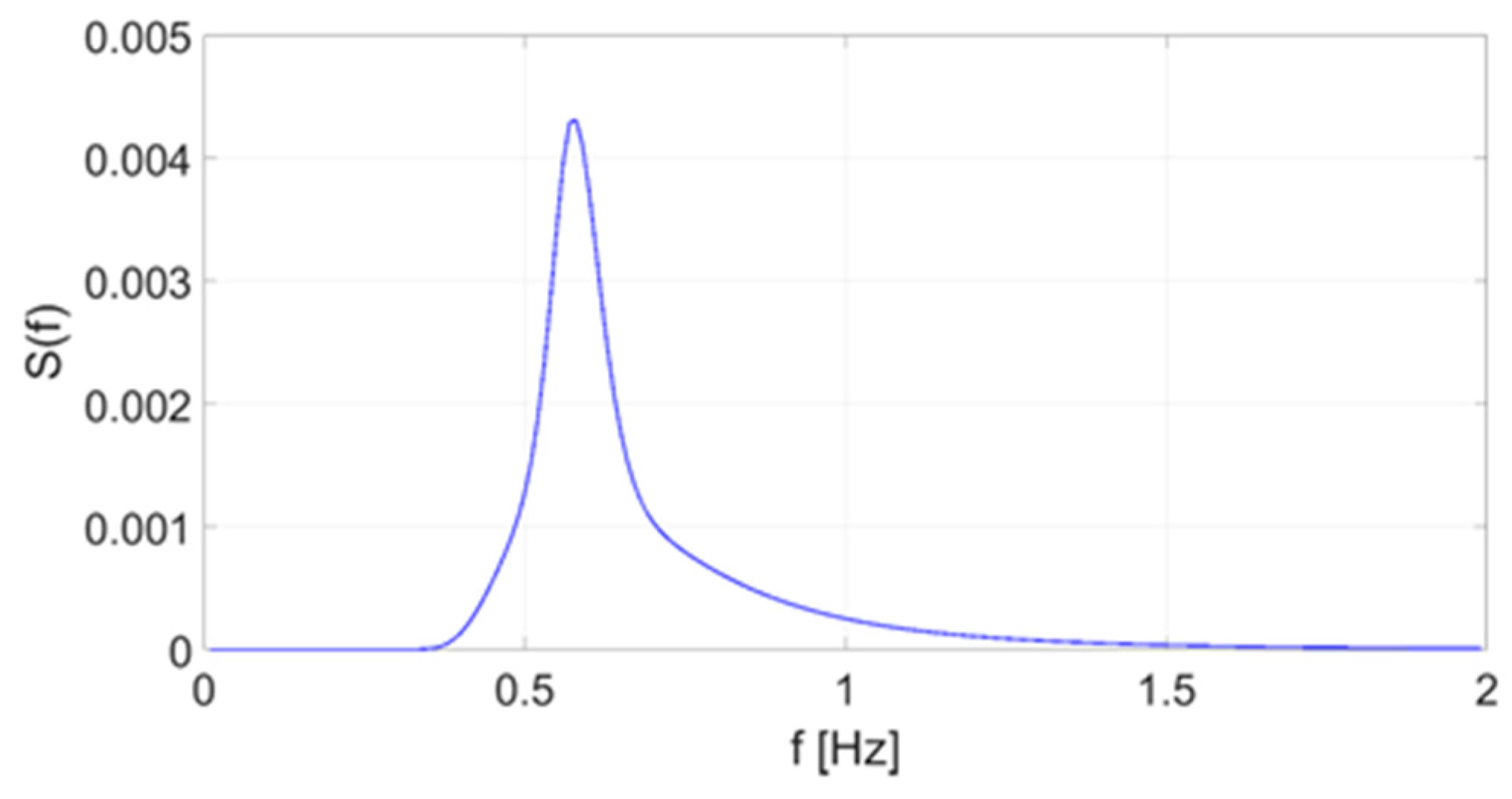
The sea surface is characterized by irregular waves that can be effectively described by the superposition of sinusoidal waves of various amplitudes, frequencies, and phases that follow a given statistical distribution. It has been shown [26] that the average energy of a wave train is proportional to the mean value of the square of the free surface elevation. Therefore, it is possible to relate the energy of a single sinusoidal component to its wave height and represent the energy of an irregular wave composed of waves of different amplitudes and frequencies through an energy spectrum. In this study, a JONSWAP-type spectrum is used [27], whose density spectrum function is

$$S\left(f\right)=C_J{H}_s{}^2\frac{f_p{}^4}{f^5}\exp \left[-\frac{5}{4}{\left(\frac{f_p}{f}\right)}^4\right]{\gamma }^b$$

(8)

where $S\left(f\right)$ is the quantity such that $S\left(f\right)df$ gives the specific energy (energy divided by the horizontal area and $\rho g$) of the waves with a frequency between $f$ and $f+df$; $H_s$ is the characteristic wave height, which is defined as $H_s=4\sqrt{m_0}$, where $m_n={{\displaystyle \int }}_0^{\infty }{f}^{n}S\left(f\right)df$ is the $n_{th}$ moment of the spectrum [16]; $f_p$ is the peak frequency; $\gamma$ is the so-called enhancement factor (in this study assumed equal to 3.3); $b$ is the exponent defined by the following expression:

$$b=\exp \left\{-\frac{1}{2}{\left(\frac{f/f_p-1}{\sigma }\right)}^2\right\};\sigma =\{\begin{array}{c}0.07 se f<f_p\\ 0.09 se f>f_p\end{array}$$

(9)

and $C_J$ is a constant required to obtain the predetermined total specific energy of the irregular wave. In the present study, $H_s$ is calculated by imposing that the $0_{th}$ moment of the spectrum, which is equal to the specific energy of the irregular wave, is equal to the specific energy of the corresponding regular wave, which is given by $\frac{1}{8}{H}^2$ [17]:

$$H_s=4\sqrt{m_0}=4\sqrt{\frac{1}{8}{H}^2}=\sqrt{2}H$$

(10)

where $H$ is the height of the regular wave. The frequency peak of the spectrum, $f_p$, is calculated from the regular wave period, $T$, by the relationship between the $0_{th}$ and the $-1_{th}$ moment of the spectrum [16]:

$$T=\frac{m_{-1}}{m_0}=0.903T_p,\mathrm{from}\mathrm{which}\mathrm{we}\mathrm{obtain}{T}_p=1.107T$$

(11)

The constant $C_J$ is evaluated by imposing that the area under the spectrum (which gives the specific total energy of the irregular wave) is equal to the specific energy of the corresponding regular wave:

$$C_J=\frac{H^2/8}{{{\displaystyle \int }}_0^{\infty }\left(H_s{}^2\frac{f_p{}^4}{f^5}\exp \left[-\frac{5}{4}{\left(\frac{f_p}{f}\right)}^4\right]{\gamma }^b\right)df}=0.205$$

(12)

Figure 1 shows the JONSWAP spectrum of an irregular wave (designed to have the same energy as a regular one) with a wave height equal to 0.08 m and wave period equal to 1.92 s.

2.3. Evaluation of the Hydrodynamic Efficiency

The hydrodynamic efficiency of the OWC device is evaluated through its capture ratio, which is given by the ratio between the average mechanical power absorbed by the OWC in a given period, $P_{OWC}$, and the mean mechanical power that is transmitted to the water column by the undisturbed wave, during the same period, $P_{wave}$,

$$\zeta =\frac{P_{OWC}}{P_{wave}}$$

(13)

where $\zeta$ can range between 0 (if the OWC device does not absorb any of the power transmitted by the waves) and 1 (if it completely absorbs that power).

2.3.1. Evaluation of the Power Transmitted by the Waves

In this paper, the evaluation of the average power transmitted to the water column during a given time interval by a regular or irregular wave is carried out by the values of water velocity and pressure obtained from the numerical simulation. In fact, it is known [17] that, during a generic time interval $\Delta t$ characterized by the passage of regular or irregular waves, the mean mechanical power transmitted to the water column (per unit length of the wavefront) through a vertical section is given by the time-averaged integral over the water column of the product between the pressure, $p$, and the horizontal velocity component, $u$:

$$P_{wave}=\frac{1}{\Delta t}{{\displaystyle \int }}_t^{t+\Delta t}{{\displaystyle \int }}_{-h}^{\eta }pudzdt$$

(14)

In the case of regular wave trains characterized by a single wave period $T$, the adopted time interval $\Delta t$ may coincide with the wave period $T$; in the case of irregular wave trains, the time interval $\Delta t$ is chosen sufficiently long to include a significant number of free surface oscillations around the still water level.

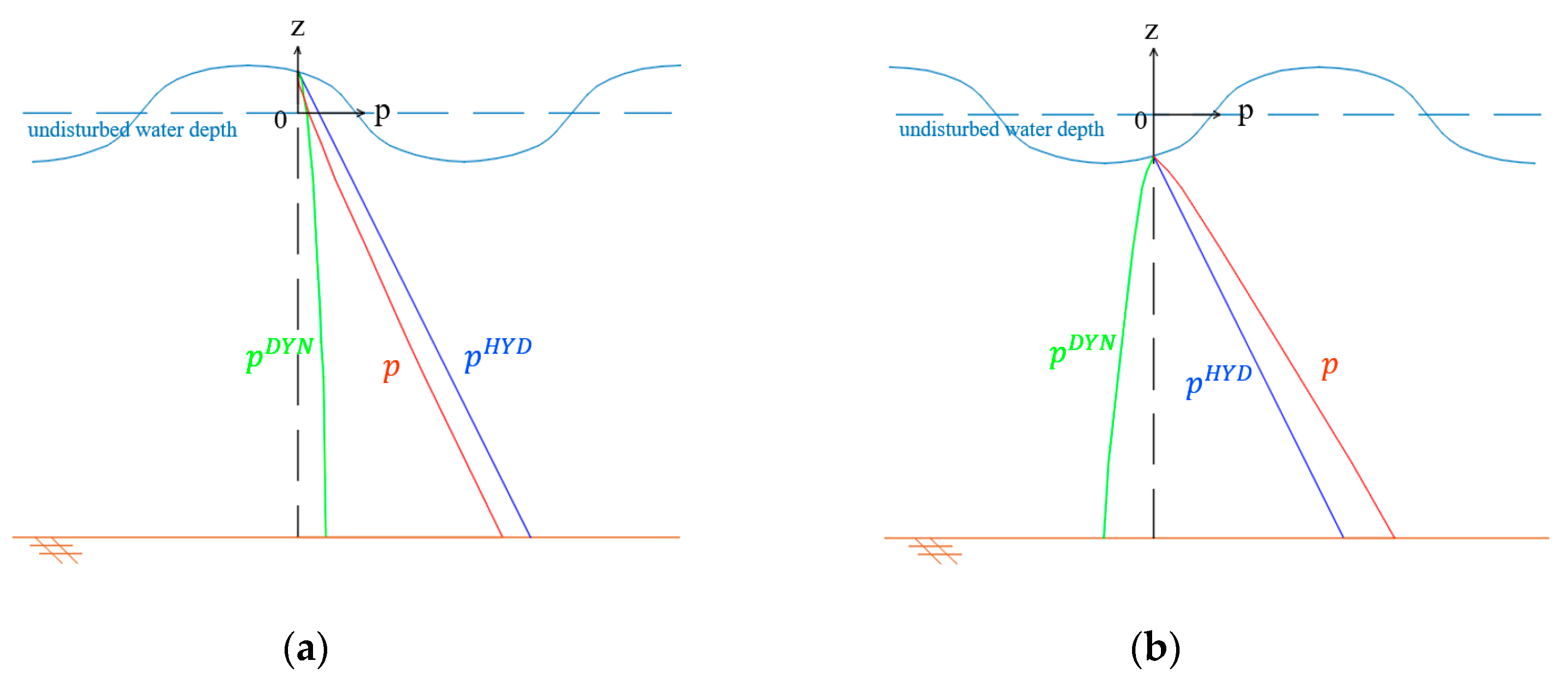
In the proposed model, the total pressure $p$ is given by the difference between a hydrostatic component, $p^{HYD}=\rho g\left(\eta -x^2\right)$, and a dynamic one, $p^{DYN}$. The latter, which is calculated by a predictor-corrector procedure, has a fundamental role in the transmission of the wave energy up to the OWC device: in the deep water region, the dynamic component is more than 10% of the hydrostatic component and is positive under the crests and negative under the trough. A scheme of the distribution of the pressure components under a wave is shown in Figure 2.

In the case of regular waves, the power transmitted by a wave to the water column can be found analytically using the expression derived from the linear wave theory [17], which gives the following relationship:

$$P_{wave}=\frac{1}{16}\rho g\frac{L{H}^2}{T}\left(1+\frac{2kd}{\sinh 2kd}\right)$$

(15)

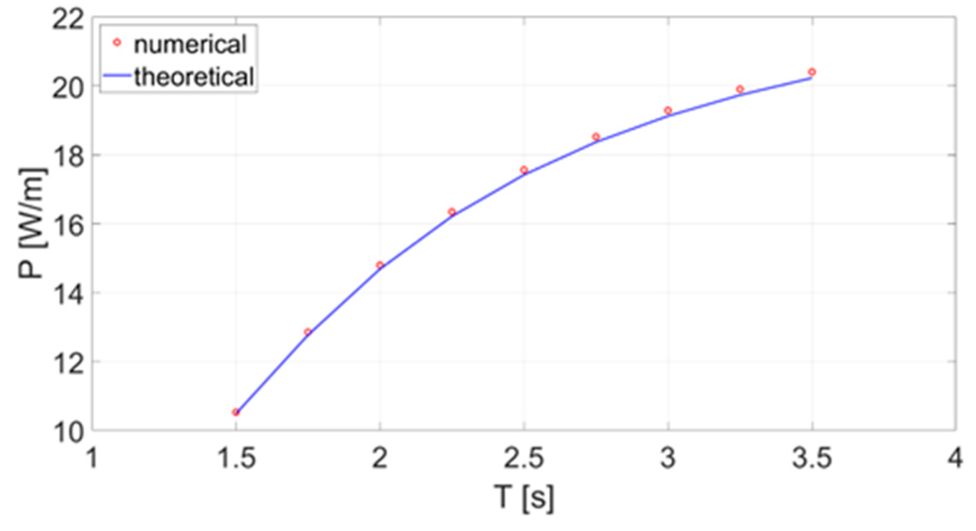
in which $L$ is the wavelength, $H$ is the wave height, $T$ is the wave period, $k=2\pi /L$ is the wave number, and $d$ is the undisturbed water depth. This expression can be used to validate the effectiveness of the proposed numerical model to generate input waves that transmit a given power to the water column. In Figure 3, it is shown a comparison between the values of the power transmitted by undisturbed regular waves calculated by the theoretical expression given by Equation (15) and the corresponding values calculated by Equation (14), in which the instantaneous values of $p$ and $u$ along the water column are obtained by the proposed model.

The good agreement between the numerical and theoretical results shows that the proposed numerical model can correctly simulate the velocity and pressure fields produced by a given wave and the transmission of its mechanical energy to the water column.

2.3.2. Evaluation of the Mechanical Power Absorbed by the OWC Device

In this paper, the evaluation of the power absorbed by the OWC device is performed by taking into account, in a fully coupled manner, the interaction between the wave motion and the air pressure inside the air chamber. In the proposed model, at each time step of the simulation, the variations of the free surface elevation inside the air chamber modify the volume of the chamber and the velocity of the air flowing through the air duct; in turn, the transit of air through the duct modifies the air pressure inside the air chamber. These pressure variations, which modify the dynamic pressure boundary condition of the free surface, can hinder or increase the water oscillations inside the air chamber. In the case in which a Wells turbine is used, as in the present study, it is possible to assume a linear relationship [28,29,30] between the difference of pressure inside and outside the air chamber and the velocity of the air flowing through the duct. Following Ning et al. [31] and Koo et al. [32], the air pressure difference inside and outside the chamber is calculated as

$$\Delta p=\left(p_{int}-p_{ext}\right)=wC$$

(16)

where $p_{ext}$ and $p_{int}$ are the pressure outside (equal to the atmospheric one) and inside the air chamber, respectively; $w$ is the velocity of the air passing through the duct, and $C$ is a constant that depends on the characteristics of the turbine and used numerical model. In [31], the constant $C$ is assumed to be equal to $3.5 \mathrm{Kg}/{\mathrm{m}}^2\mathrm{s}.$ In the present study, a value of $3.8 \mathrm{Kg}/{\mathrm{m}}^2\mathrm{s}$ is chosen for the constant $C$, which provides a better agreement between the numerical results and the experimental data. The velocity $w$ at the air duct inlet is calculated through the equation

$$w=\frac{\Delta V}{A\Delta t}$$

(17)

where $\Delta V$ is the change of the air volume in the chamber during a time interval $\Delta t$ and $A$ is the sectional area of the air duct. In this paper, according to [31,32], the effect of air compressibility is considered negligible, and consequently, the changes in the air volume in the chamber are calculated as a function of the free-surface variations.

The mean mechanical power absorbed by the OWC in a time interval $\Delta t$ is given by the time average of the product between the air flow rate in the duct and the difference of pressure inside and outside the air chamber:

$$P_{OWC}=\frac{1}{\Delta t}{{\displaystyle \int }}_t^{t+\Delta t}Q\left(t\right)\Delta p\left(t\right)dt$$

(18)

where $Q\left(t\right)=w\left(t\right)A$ is the airflow rate in the duct. By considering Equation $\left(16\right)$, it is possible to rewrite Equation (18) as

$$P_{OWC}=\frac{1}{\Delta t}{{\displaystyle \int }}_t^{t+\Delta t}w\left(t\right)w\left(t\right)ACdt=\frac{AC}{\Delta t}{{\displaystyle \int }}_t^{t+\Delta t}{w}^2\left(t\right)dt$$

(19)

3. Results

This section is divided in three subsections: in the first one, the proposed model is validated against an experimental test regarding the efficiency of a laboratory-scale OWC by Morris-Thomas [25], which used regular waves; in the second subsection, the proposed model is used to calculate the performance of the same OWC device under more realistic conditions given by irregular wave trains characterized by the same wave energy of the regular ones used for the validation; in the third subsection, the proposed model is applied to evaluate the potential energy production obtainable from the waves by using a set of OWCs placed along the breakwater that protects the Cetraro harbor in southern Italy.

3.1. Validation of the Numerical Model

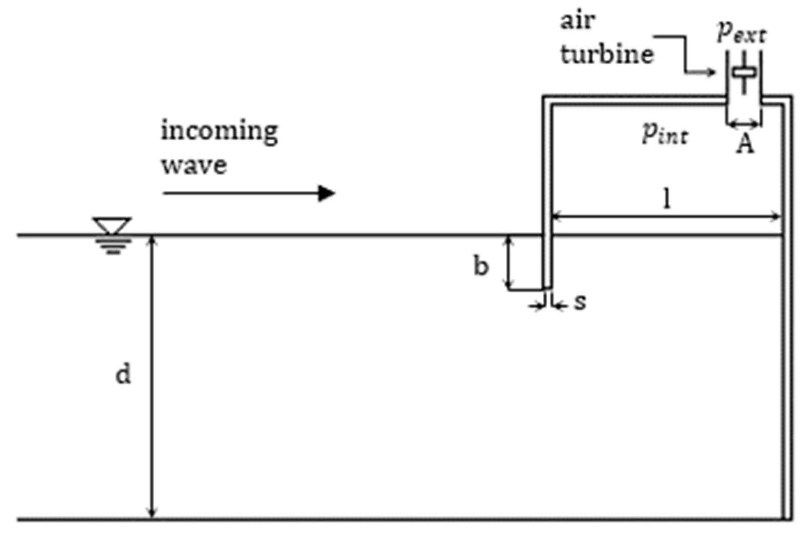
In order to validate the numerical model, data from an experimental laboratory study by Morris-Thomas et al. [25] were used. This laboratory study involved a 1:12.5 scale model of an OWC device, which was placed at the end of a wave tank with a geometry similar to a commercial prototype used at Port Kembla on Australia’s east coast. The distance between the wave maker and the device was about 38 m; the undisturbed water depth $d$ was 0.92 m, and the wave height $H$ was 0.08 m. The pressure variation inside the chamber due to the power take-off was modeled through a vent, with a width A $=0.005 \mathrm{m}$, which crossed the entire upper wall of the OWC device. The air chamber had a length of $l=0.64 \mathrm{m}$ in the wave propagation direction; the thickness and draught of the front wall were, respectively, $s=0.04 \mathrm{m}$ and b $=0.15 \mathrm{m}$ (see Figure 4 and

Table 1. Values of the geometric parameters of the experimental test used to validate the proposed numerical model.

d	0.92	m
b	0.15	m
s	0.04	m
l	0.64	m
a	0.005	m

).

In the numerical simulations, the geometrical configuration of the experimental test was reproduced by using a spatial discretization step, $dx=0.04 \mathrm{m}$, in the horizontal direction and 13 layers in the vertical direction.

The comparison between the experimental and numerical results was carried out by calculating the hydrodynamic efficiency of the OWC, which is given by the ratio between the mechanical power absorbed by the device and the power transmitted by the incident wave for different values of the dimensionless deep-water wave number, $K_d$. The latter is defined as

$$K_d=kd\tanh \left(kd\right)$$

(20)

where $d$ is the still water depth; $k=2\pi /L$ is the wave number of the incident wave, and $L$ is the wavelength, which is calculated iteratively by using the linear wave theory:

$$L=\frac{g{T}^2}{2\pi }\tanh \left(2\pi \frac{d}{L}\right)$$

(21)

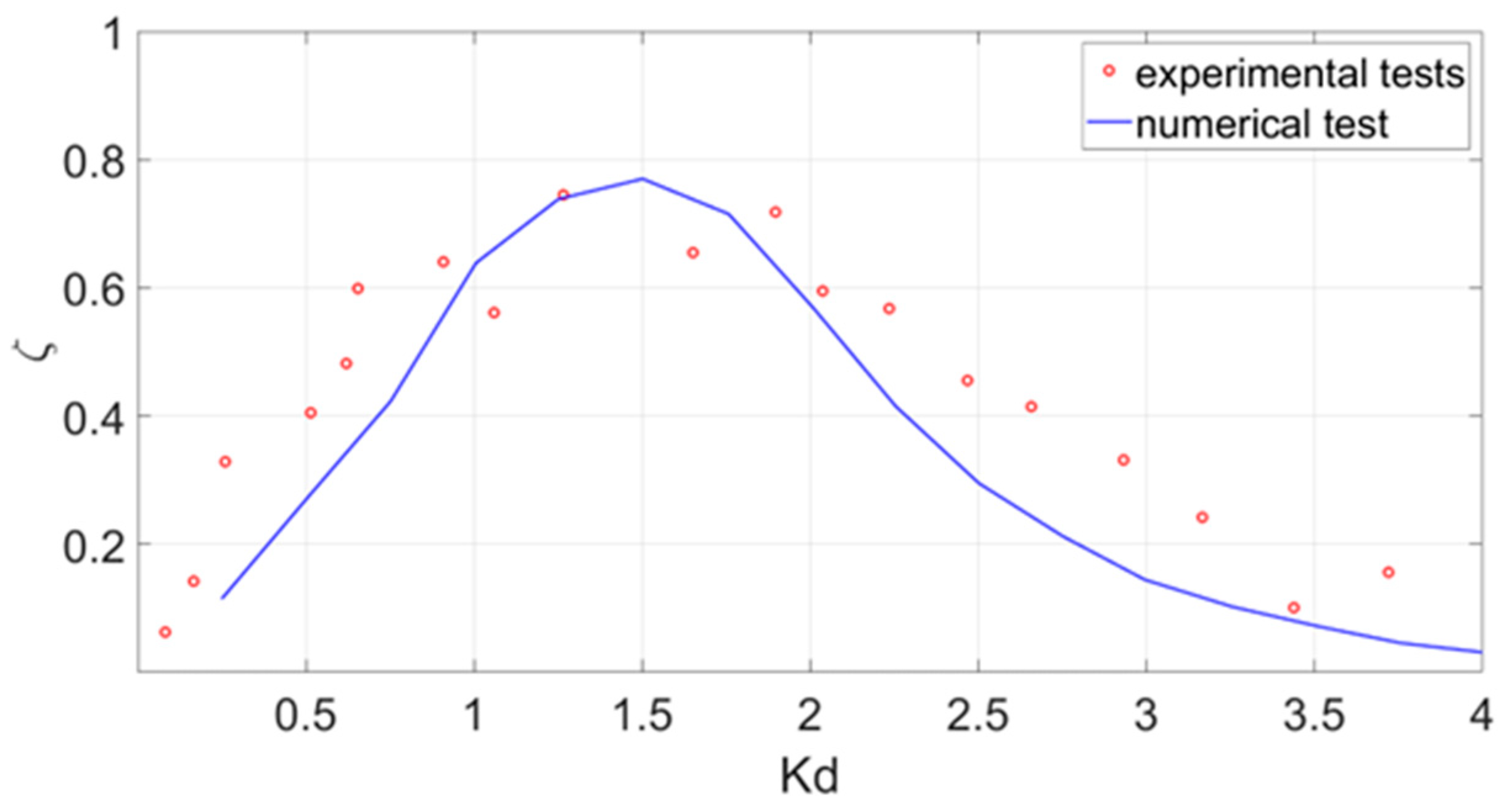
Figure 5 shows the comparison between the OWC hydrodynamic efficiency obtained by the experimental data and the one calculated through the numerical simulations for different wave numbers. A good agreement is found between the experimental values and the numerical ones for all the wave numbers. From both the experimental and numerical results, it is evident that the hydrodynamic efficiency of the OWC has a maximum of about 78% near $K_d=1.5$ (corresponding to a wave frequency of 0.64 Hz and a wavelength of 3.56 m).

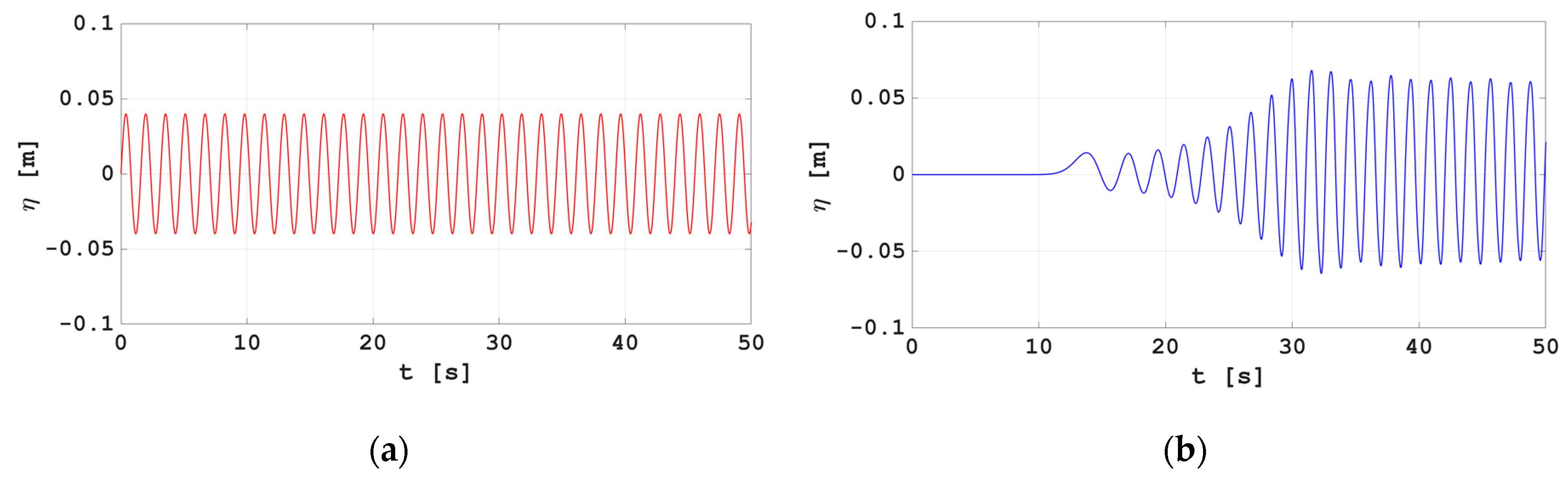
As shown by the numerical results obtained by using the proposed model, this maximum hydrodynamic efficiency is due to resonance phenomena in the air chamber of the OWC: for a given specific wave frequency and wavelength of the incoming waves, the part of the wave that is transmitted inside the air chamber due to the reflections by the internal walls induces a periodic amplification of the water column oscillations in the air chamber that is in phase with the incoming waves. After that, no less than 10 incoming waves with the same period (and wavelength) have reached the air chamber; these in-phase amplification phenomena produce the final maximum increment of the wave amplitude inside the air chamber. In these conditions, the maximum mechanical power absorption in the air chamber and OWC hydrodynamic efficiency take place. This behavior is highlighted in Figure 6, which shows the first 50 s of the time history of the free-surface elevation (for the wave corresponding to the efficiency peak) at the generation point (Figure 6a) and at the center of the air chamber (Figure 6b).

Inside the air chamber, a transitory occurrence of about 10 waves induces an increase in the free-surface oscillations, from about $\pm 0.02$ m to about $\pm 0.06$ m, with a consequent final improvement in mechanical power absorption and OWC hydrodynamic efficiency. It must be emphasized that, in order to obtain this final result, the incoming waves should have the same geometric characteristics during the considered time interval. This situation hardly occurs in natural conditions, where the real waves have randomly distributed wave characteristics.

3.2. Hydrodynamic Efficiency of the OWC Device under Irregular Waves

In many of the studies on the OWC hydrodynamic efficiency [10,11,12,13,14,15], the wave trains interacting with these devices are composed of sinusoidal monochromatic waves. This simplification is unrealistic and, as discussed above, may lead to an overestimation of OWC performance. In this subsection, the proposed numerical model was applied to the study of OWC performance in the presence of irregular waves. In order to quantify any overestimation of the OWC hydrodynamic efficiency due to the use of regular waves, all the simulations performed to validate the model were repeated by using irregular waves defined by JONSWAP spectra, characterized by the same total energy of the corresponding regular waves. The simulation time for all the irregular wave cases is not less than 600 s, which corresponds to more than 100 waves identified by the zero-crossing technique.

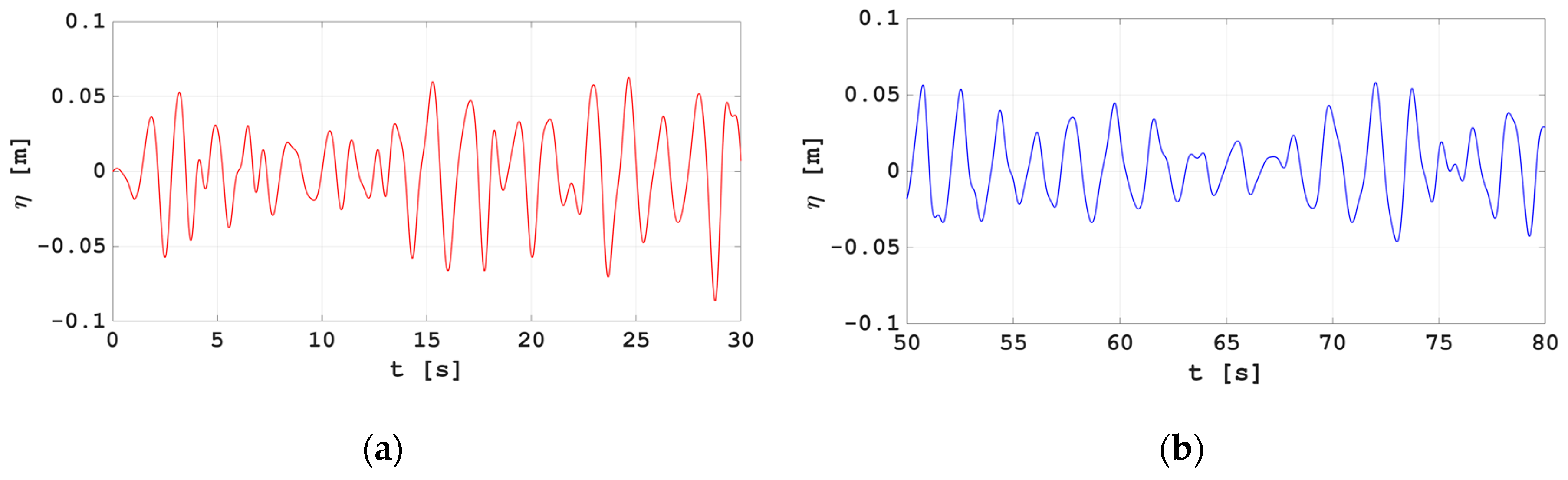
Figure 7 shows a small portion (30 s) of the time series of the free-surface elevation at the generation point (Figure 7a) and at the center of the air chamber (Figure 7b) for the irregular wave train corresponding to the regular one, which provides maximum OWC hydrodynamic efficiency $\left(K_d=1.5\right)$.

Figure 7b shows that, in the case of the irregular wave train, the wave amplitudes inside the air chamber are characterized by significant variability and are similar to the ones outside the OWC that do not favor the onset of resonance conditions. This result is very different from the one obtained by using regular waves (Figure 6b), in which resonance conditions favor the amplification of the free-surface oscillation during the entire simulated time interval.

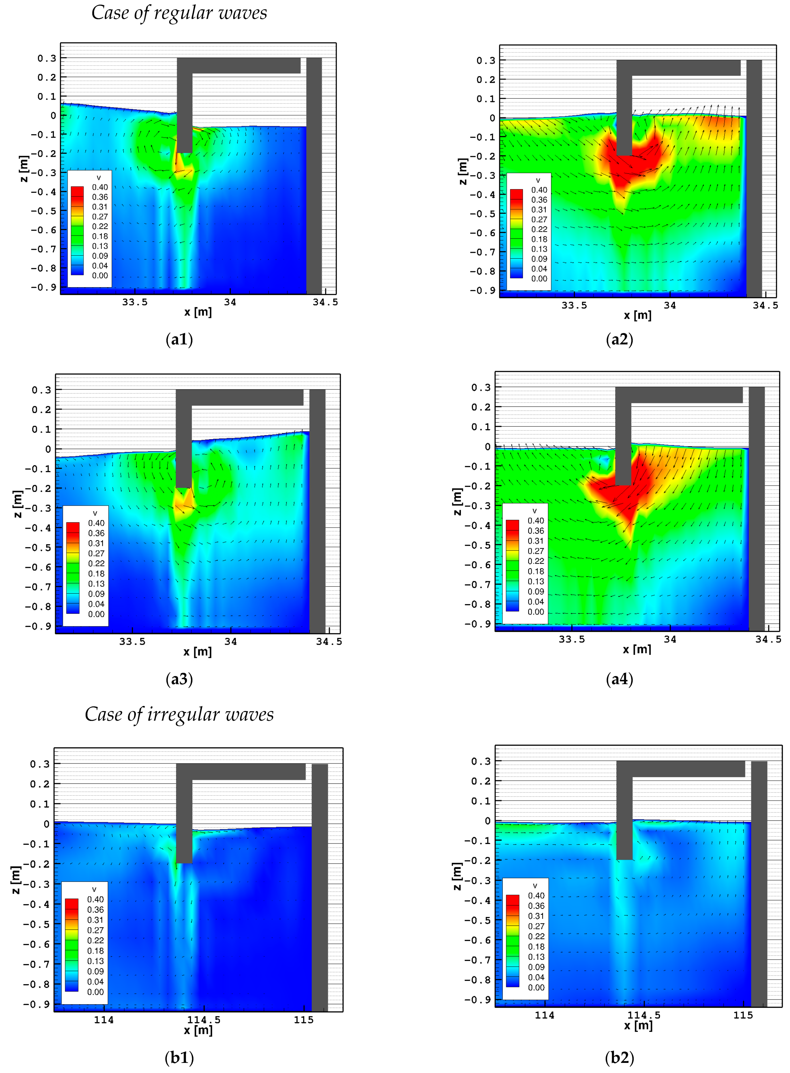
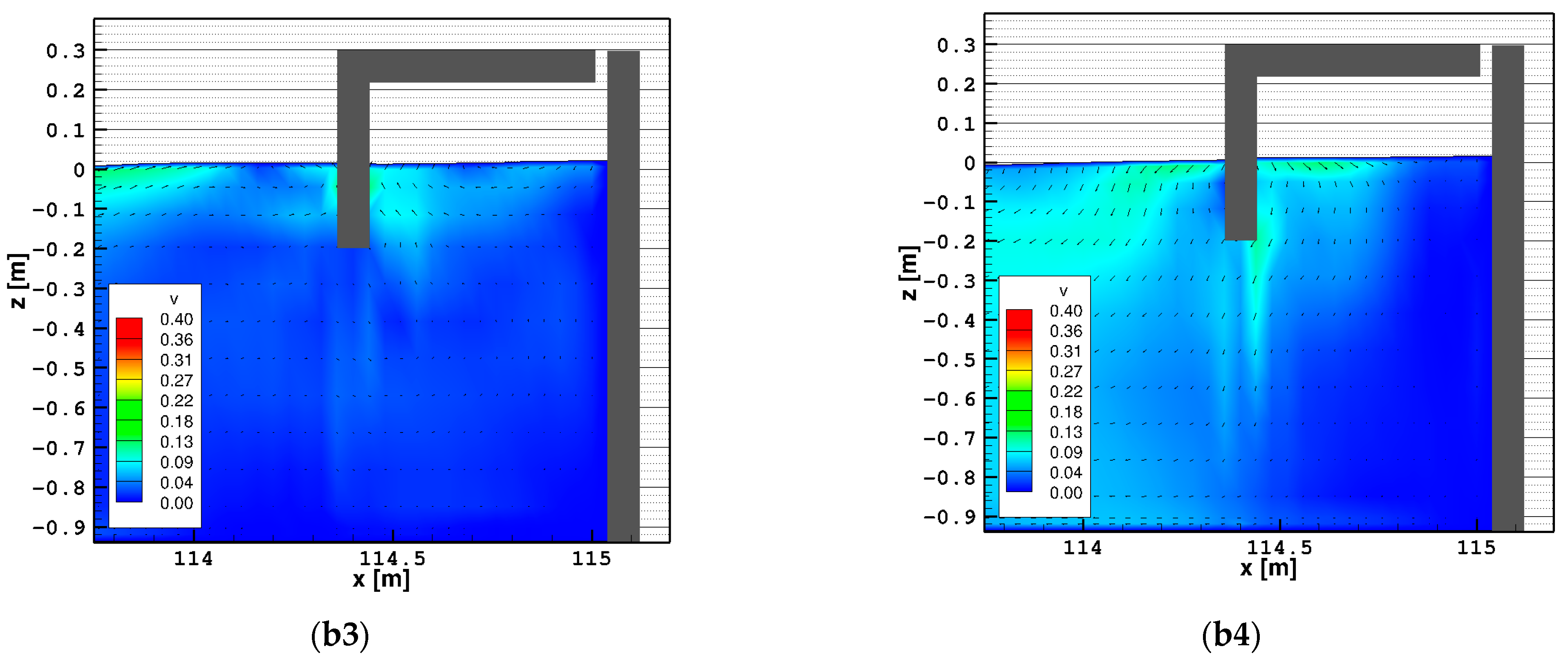
The differences between the hydrodynamics inside the chamber produced by the regular wave train and by the corresponding irregular one are highlighted in Figure 8, where two sequences of the instantaneous velocity and free-surface elevation fields are shown: the first sequence shows the results obtained by adopting the regular wave train, which provides maximum hydrodynamic efficiency (Figure 8a); the second sequence shows the results obtained by using the corresponding irregular one (Figure 8b). The comparison of the two sequences shows that, in the case of regular waves, the periodic free-surface elevation gradients between the outside and inside of the air chamber produce water velocities that are significantly greater than those occurring in the case of irregular waves. In this latter case, there are several time intervals in which the wave energy transmission inside the air chamber is significantly less than in the regular wave case, with a consequent decrease in hydrodynamic efficiency from 0.78 to about 0.54.

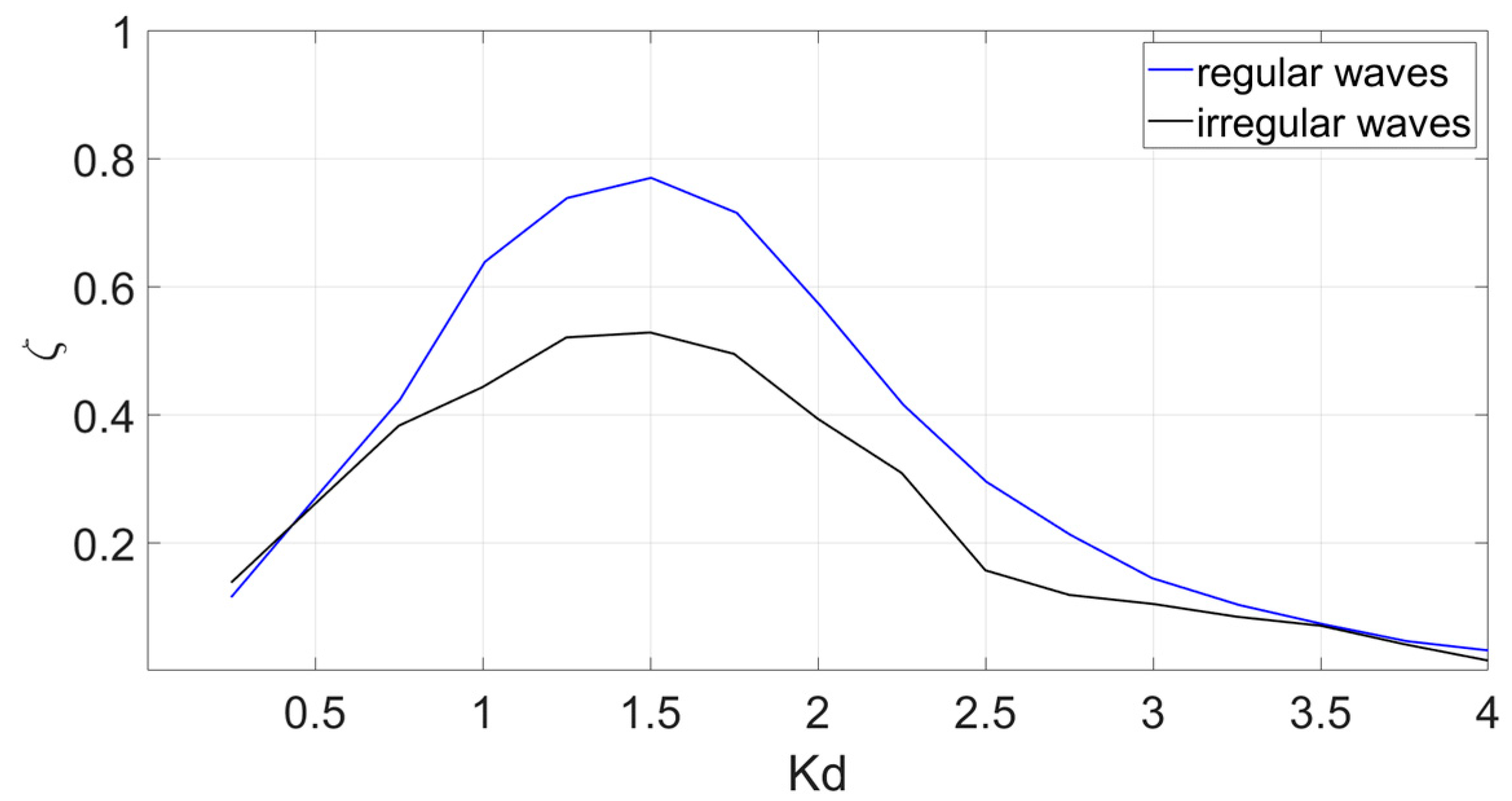
In this work, in order to find the irregular wave train that produces maximum hydrodynamic efficiency, all the numerical simulations carried out to produce the graph in Figure 5 were repeated by using irregular wave trains characterized by the same energy as the corresponding regular ones. The comparison between the hydrodynamic efficiency obtained by using regular and irregular wave trains is shown in Figure 9. This figure shows that the variation in the hydrodynamic efficiency as a function of the deep-water wave number of the incident waves is similar in the two cases and that the peak efficiency of the device occurs for the same dimensionless deep-water wave number. The comparison between the two curves highlights that the hydrodynamic efficiency obtained by using irregular wave trains is significantly lower than the one obtained by the corresponding regular ones, with a maximum decrease of about 25% at the efficiency peak.

In conclusion, the numerical results obtained by the proposed model show that the hydrodynamic efficiency calculated by considering regular waves can be significantly overestimated with respect to the one calculated by considering irregular waves. This demonstrates the fact that, for a more reliable assessment of the expected device efficiency, it is necessary to refer to the values obtained by using irregular waves.

3.3. Evaluation of the Potential Energy Production Obtainable by OWCs at Cetraro Harbor

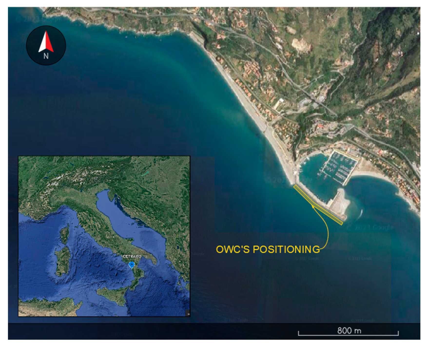
In this section, the proposed numerical model is used to estimate the potential energy production obtainable by a set of OWC devices at Cetraro harbor (Southern Italy). The Cetraro harbor (Figure 10) is protected by a straight breakwater parallel to the coastline, which extends for about 500 m in the southeast direction.

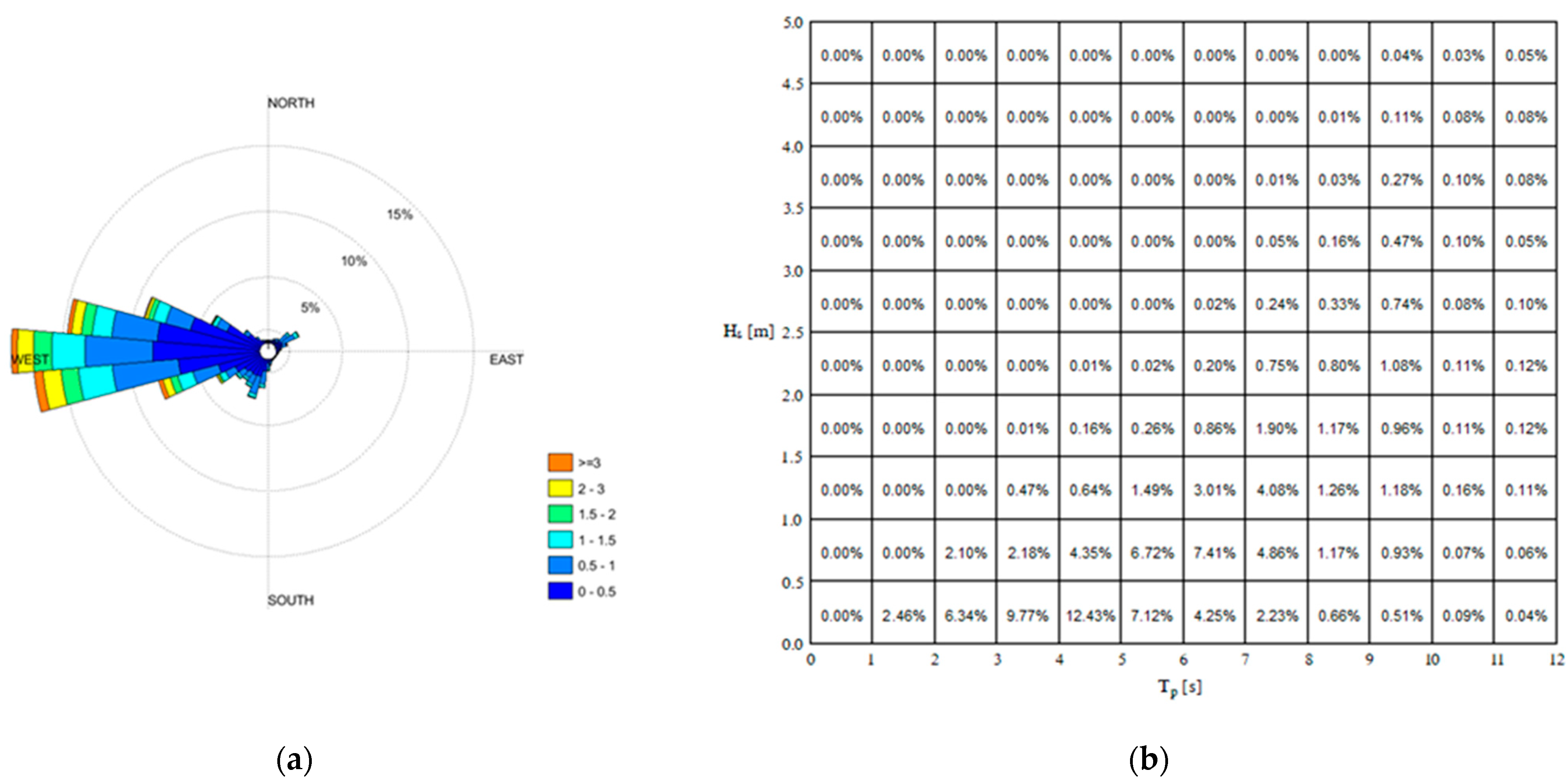
In order to characterize the prevailing wave regime at the Cetraro harbor, the data from a measurement campaign carried out by the Cetraro buoy of the Italian National Ondametric Network (RON), installed offshore Cetraro and active from 1999 to 2014, were processed. Figure 11 shows the directional distribution and the joint probability distribution between peak period $T_p$ and significant wave height $H_s$ obtained as a result of data processing. Figure 11a shows that most of the waves propagate from west to east. Figure 11b shows that the waves with a higher frequency of occurrence are relatively small, with a significant wave height between 0 and 1, as is typical on the coasts of the Mediterranean Sea.

For the evaluation of the potential energy production obtainable at this site, the installation of a set of OWC devices integrated into the breakwater for 400 m is assumed. The use of Wells turbines with a constant efficiency of 0.5 (for full-size turbines, the peak efficiency is 0.7–0.8 [4]) in the power take-off system is also assumed.

When using the proposed model, a series of numerical simulations are performed by generating irregular waves with JONSWAP-type spectra and wave characteristics derived from the buoy data. The generation point of these waves is located at a distance of 1500 m from the breakwater, where the water depth is 50 m, and the wave characteristics are the ones shown in Figure 11. For the present study, waves with a height of greater than 2 m are not considered because they are associated with extreme events. The remaining data were subdivided into four groups, from which four different irregular input waves were obtained: the first group includes all the recorded data relative to those waves with a height between 0 m and 0.5 m; the second one includes the waves with a height of between 0.5 m and 1 m; the third group includes the waves with a height of between 1 m and 1.5 m; the fourth group includes the waves with a height of between 1.5 m and 2 m. The mean significant wave height and peak period of each group are shown in

Table 2. Mean mechanical power absorbed by the device for different irregular wave characteristics: $H_s$ is the significant wave height, $T_p$ is the peak period, and $P_{prod}$ is the mean mechanical power absorbed per unit of length of the wavefront.

$${\mathit{H}}_{\mathit{s}}\left[\mathbf{m}\right]$$	$${\mathit{T}}_{\mathit{p}}\left[\mathbf{s}\right]$$	$${\mathit{P}}_{\mathit{p}\mathit{r}\mathit{o}\mathit{d}}[\mathbf{W}/\mathbf{m}]$$
0.29	4.51	545.44
0.72	5.88	3264.33
1.22	7.11	5010.10
1.72	7.89	5330.71

. Such wave parameters are used to generate the JONSWAP spectrum of the irregular input waves in the numerical simulations for the interaction between the waves and the OWC at Cetraro harbor. The numerical simulations relative to each irregular input wave are repeated for the different geometric characteristics of the OWC device in order to maximize the mean annual mechanical power absorption at Cetraro harbor for the given wave regime. The final chosen geometric characteristics were 6 m for the air chamber length (in the wave propagation direction) and 0.75 m for the front wall draught.

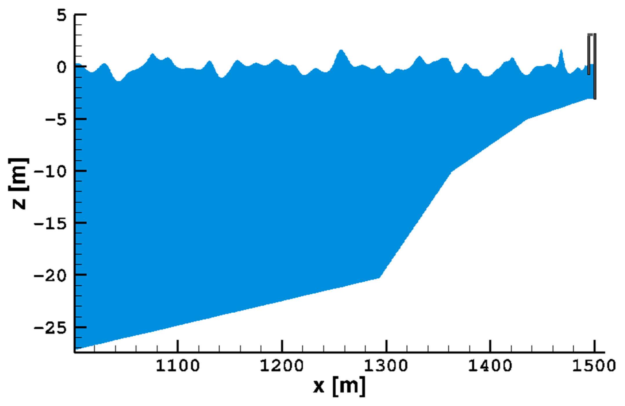
Figure 12 shows a detail of the instantaneous wave field obtained by the numerical simulation of the irregular waves with a significant wave height of 1.22 m and a peak period of 7.11 s.

In the last column of Table 2, the mean mechanical power absorption per unit of the length of the wavefront obtained by the numerical simulations relative to each irregular input wave is reported.

From Table 2, it is possible to note that, for the given geometric characteristics of the air chamber, the mechanical power absorption of the OWC device increases with the increase in the height of the incoming waves, and it is maximum for the waves belonging to the fourth group ($H_s=1.72 \mathrm{m}$), whose occurrence frequency is lower than 6% per year. From the same table, it can be noted that the mechanical power absorption is also close to the maximum for the waves belonging to the third group ($H_s=1.22 \mathrm{m}$), whose frequency is 12% per year, and also is significant for the waves of the second group ($H_s=0.72 \mathrm{m}$), whose frequency (30% per year) is considerably higher than the waves belonging to the fourth group. This implies that, at Cetraro harbor, significant power production can be obtained not only during the less frequent and intense storm surges but also during more common sea conditions. Furthermore, by summing the power contributions of each wave group multiplied by its mean occurrence time and by the length of the OWC plant (400 m), the estimation of the mean annual energy production obtainable at Cetraro harbor is about 1540.52 MWh. This value corresponds to the energy production of about 10 wind turbines with a nominal power of 60 KW, confirming the competitiveness of wave energy with respect to other renewable sources, even in areas such as the Mediterranean Sea, where waves do not possess a high energy potential.

It must be emphasized that by changing the length of the air chamber (in the wave propagation direction) with respect to the chosen one (6 m) the mean annual power absorption obtained by the numerical simulations does not increase. This result is observed not only by adopting a shorter air chamber length but also by using a longer one. In fact, by using an air chamber length equal to 7 m, a decrease in the mechanical power absorption associated with the smaller and more frequent waves (first and second group in Table 2) can be observed, which is only just compensated for by an increase in the mechanical power absorption associated with the bigger and less frequent waves (third and fourth group in Table 2). The resulting mean annual energy production is almost the same as the one obtained by using an air chamber length of 6 m. This effect is even more evident for an air chamber length greater than 7 m: in this case, the reduction in the mechanical power absorption associated with the smaller and more frequent waves is superior to the increase in power absorption associated with the bigger and less frequent waves. This implies an overall reduction in mean annual energy production for an air chamber length greater than 7 m.

4. Conclusions

A numerical investigation into the hydrodynamic performance of an oscillating water column device is proposed. The numerical simulations were carried out by using a two-dimensional free-surface nonhydrostatic numerical model that is based on the contravariant form of the Navier–Stokes equations expressed in a moving co-ordinate system. The proposed model was used to simulate wave propagations and interactions with the OWC device and to evaluate its mechanical power absorption for different geometric characteristics regarding the air chamber and different wave conditions. By using the proposed model, the performances of the OWC devices obtained by using regular waves were compared to those obtained by using irregular waves characterized by the same energy as the regular ones. The results of the numerical simulations show that the hydrodynamic efficiency calculated by using regular waves can be significantly overestimated with respect to those obtained by more realistic irregular waves. Finally, the model was applied to the evaluation of the potential energy production obtainable from the waves by using a set of OWCs placed along the breakwater that protects the Cetraro harbor in southern Italy. The numerical results show that, for the prevailing wave regime of the Cetraro harbor, the optimal air chamber length is equal to 6 m; greater lengths of the air chamber produce a reduction in the power absorption associated with the smaller and more frequent waves, which is not compensated for by the increase in power absorption associated with the bigger and less frequent waves. By adopting the optimal dimensions, the estimated mean annual energy production obtainable at the Cetraro harbor is equal to 1540.52 MWh, which corresponds to the energy production of about 10 wind turbines with a nominal power of 60 KW. These results show the competitiveness of wave energy with respect to other renewable sources, even in areas such as the Mediterranean Sea, where waves do not possess a high energy potential.

Future work on this issue will focus on removing some of the assumed simplifications in the adopted model, such as the incompressibility of the air inside the chamber, and on increasing the accuracy of the numerical solution on coarse computational grids that are usually adopted for real-scale simulations. For that purpose, a new line of research will be concerned with the development and adoption of a more complex turbulence model than the Smagorinsky one (which is strictly dependent on the spatial grid step) in order to reduce energy dissipation and improve the numerical results on coarse computational grids. Furthermore, future numerical investigations will regard the comparison between different types of wave energy converters.

References

- Gunn, K.; Stock-Williams, C. Quantifying the global wave power resource. Renew. Energy 2012, 44, 296–304. [Google Scholar] [CrossRef]
- Falcão, A.F.O.; Henriques, J.C.C. Oscillating-water-column wave energy converters and air turbines: A review. Renew. Energy 2016, 85, 1391–1424. [Google Scholar] [CrossRef]
- Falcão, A.F.O. Overview on Oscillating Water Column Devices. Mater. Res. Proc. 2022, 20, 9781644901731-1. [Google Scholar]
- Gato, L.M.C.; Falcão, A.F.O. Aerodynamics of the wells turbine. Int. J. Mech. Sci. 1988, 30, 383–395. [Google Scholar] [CrossRef]
- Suzuki, M.; Arakawa, C. Guide vanes effect of wells turbine for wave power generator. Int. J. Offshore Polar Eng. 2000, 10, 153–159. [Google Scholar]
- Ning, D.; Zhou, Y.; Mayon, R.; Johanning, L. Experimental investigation on the hydrodynamic performance of a cylindrical dual-chamber Oscillating Water Column device. Appl. Energy 2020, 260, 114252. [Google Scholar] [CrossRef]
- Çelik, A.; Altunkaynak, A. Experimental investigations on the performance of a fixed-oscillating water column type wave energy converter. Energy 2019, 188, 116071. [Google Scholar] [CrossRef]
- Ram, K.; Faizal, M.; Ahmed, M.R.; Lee, Y. Experimental studies on the flow characteristics in an oscillating water column device. J. Mech. Sci. Technol. 2010, 24, 2043–2050. [Google Scholar] [CrossRef]
- Ning, D.; Wang, R.; Zou, Q.; Teng, B. An experimental investigation of hydrodynamics of a fixed OWC Wave Energy Converter. Appl. Energy 2016, 168, 636–648. [Google Scholar] [CrossRef]
- Rezanejad, K.; Bhattacharjee, J.; Soares, C.G. Analytical and Numerical Study of Nearshore Multiple Oscillating Water Columns. J. Offshore Mech. Artic Eng. 2013, 8, V008T09A098. [Google Scholar]
- Kamath, A.; Bihs, H.; Arntsen, Ø.A. Numerical investigations of the hydrodynamics of an oscillating water column device. Ocean. Eng. 2015, 102, 40–50. [Google Scholar] [CrossRef] [Green Version]
- Elhanaf, A.; Fleming, A.; Macfarlane, G.; Leong, Z. Numerical hydrodynamic analysis of an offshore stationary floating oscillating water column wave energy converter using CFD. Int. J. Nav. Archit. Ocean. Eng. 2017, 9, 77–99. [Google Scholar] [CrossRef] [Green Version]
- Luo, Y.; Nader, J.; Cooper, P.; Zhu, S. Nonlinear 2D analysis of the efficiency of fixed Oscillating Water Column wave energy converters. Renew. Energy 2014, 64, 255–265. [Google Scholar] [CrossRef]
- Teixeira, P.R.F.; Davyt, D.P.; Didier, E.; Ramalhais, R. Numerical simulation of an oscillating water column device using a code based on Navier-Stokes equations. Energy 2013, 61, 513–530. [Google Scholar] [CrossRef]
- Haghighi, A.T.; Nikseresht, A.H.; Hayati, M. Numerical analysis of hydrodynamic performance of a dual-chamber Oscillating Water Column. Energy 2021, 221, 119892. [Google Scholar] [CrossRef]
- Carter, D.J.T. Estimation of wave spectra from wave height and period. Inst. Oceanogr. Sci. 1982, 135, 1–20. [Google Scholar]
- Kundu, P.K.; Cohen, I.M.; Dowling, D.R. Gravity Waves. In Fluid Mechanics, 5th ed.; Elsevier: Waltham, MA, USA, 2012. [Google Scholar]
- Bradford, S.F. Numerical simulation of surf zone dynamics. J. Waterw. Port Costal Ocean. Eng. 2000, 126, 1–13. [Google Scholar] [CrossRef]
- Higuera, P.; Lara, J.L.; Losada, I.J. Simulating coastal engineering processes with OpenFOAM®. Coast. Eng. 2013, 71, 119–134. [Google Scholar] [CrossRef]
- Ma, G.; Shi, F.; Kirby, J. Shock-capturing non-hydrostatic model for fully dispersive surface wave processes. Ocean. Model. 2012, 43, 22–35. [Google Scholar] [CrossRef]
- Cannata, G.; Petrelli, C.; Barsi, L.; Gallerano, F. Numerical integration of the contravariant integral form of the Navier-Stokes equations in time-dependent curvilinear coordinate system for three-dimensional free surface flows. Contin. Mech. Thermodyn. 2019, 31, 491–519. [Google Scholar] [CrossRef] [Green Version]
- Elhanafi, A.; Macfarlane, G.; Fleming, A.; Leong, Z. Investigations on 3D effects and correlation between wave height and lip submergence of an offshore stationary OWC wave energy converter. Appl. Ocean. Res. 2017, 64, 203–216. [Google Scholar] [CrossRef]
- Wang, C.; Zhang, Y. Hydrodynamic performance of an offshore Oscillating Water Column device mounted over an immersed horizontal plate: A numerical study. Energy 2021, 222, 119964. [Google Scholar] [CrossRef]
- Cannata, G.; Palleschi, F.; Iele, B.; Gallerano, F. A Wave-Targeted Essentially Non-Oscillatory3D Shock-Capturing Scheme for Breaking Wave Simulation. J. Mar. Sci. Eng. 2022, 10, 810. [Google Scholar] [CrossRef]
- Morris-Thomas, M.T.; Irvin, R.J.; Thiagarajan, K.P. An Investigation into the Hydrodynamic Efficiency of an Oscillating Water Column. J. Offshore Mech. Arct. Eng. 2007, 129, 273–278. [Google Scholar] [CrossRef]
- Kinsman, B. Wind Waves: Their Generation and Propagation on the Ocean Surface; Prentice-Hall: Englewood Cliffs, NJ, USA, 1965. [Google Scholar]
- Hasselmann, K.; Barnett, T.P.; Bouws, E.; Carlson, H.; Cartwright, D.E.; Enke, K.; Ewing, J.A.; Gienapp, A.; Hasselmann, D.E.; Kruseman, P.; et al. Measurements of wind-wave growth and swell decay during the joint North Sea wave project (JONSWAP). Ergänzungsheft Zur Dtsch. Hydrogr. Z. 1973. Available online: http://resolver.tudelft.nl/uuid:f204e188-13b9-49d8-a6dc-4fb7c20562fc (accessed on 22 March 2023).
- Sheng, W.; Alcorn, R.; Lewis, A. On thermodynamics in the primary power conversion of oscillating water column wave energy converters. J. Renew. Sustain. Energy 2013, 5, 023105. [Google Scholar] [CrossRef] [Green Version]
- Curran, R.; Gato, L.M.C. The energy conversion performance of several types of Wells turbine designs. Proc. Inst. Mech. Eng. Part A J. Power Energy 1997, 211, 133–145. [Google Scholar] [CrossRef]
- Raghunathan, S. The wells air turbine for wave energy conversion. Prog. Aerosp. Sci. 1995, 31, 335–386. [Google Scholar] [CrossRef]
- Ning, D.; Shi, J.; Zou, Q.; Teng, B. Investigation of hydrodynamic performance of an OWC (oscillating water column) wave energy device using a fully nonlinear HOBEM (higher-order boundary element method). Energy 2015, 83, 177–188. [Google Scholar] [CrossRef]
- Koo, W.; Kim, M. Nonlinear Time-Domain Simulation of a Land-Based Oscillating Water Column. J. Waterw. Port Coast. Ocean. Eng. 2010, 136, 276–285. [Google Scholar] [CrossRef]
Figure 1.
JONSWAP spectrum of an irregular wave with the same energy as a regular wave with a height equal to 0.08 m and a period equal to 1.92 s.
Figure 2.
Qualitative pressure distribution along the water column: (a) under a wave crest; (b) under a wave trough. Dashed line: still water level; continuous line: instantaneous free-surface; red line: total pressure distribution; blue line: hydrostatic pressure distribution; green line: dynamic pressure distribution.
Figure 3.
Comparison of the transmitted wave power calculated by the proposed model (red dots) and by the theoretical expression given by Equation (15) (blue line).
Figure 4.
Geometric configuration of the experimental and numerical test used to validate the proposed model. is the undisturbed water depth; is the front wall draught; is the front wall thickness; is the air chamber length, and is the width of the vent on the OWC upper wall.
Figure 5.
Hydrodynamic efficiency of the OWC versus dimensionless deep-water wave number: a comparison between the experimental data (red dots) and the numerical results (blue line).
Figure 6.
Free-surface elevation versus time for the regular wave with : (a) at the generation point; (b) at the center of the air chamber.
Figure 7.
Time history of free-surface elevation of the irregular wave corresponding to the regular wave, which provides maximum hydrodynamic efficiency : (a) at the generation point; (b) at the center of the air chamber.
Figure 8.
Interaction between incident waves and the OWC device. Two different sequences of the instantaneous hydrodynamic fields were obtained under a regular wave train (Case a) and the corresponding irregular one (Case b). (a): regular wave train at 41.6 s (a1), 42 s (a2), 42.4 s (a3), and 42.8 s (a4). (b) Corresponding irregular wave train at 64.55 s (b1), 65 s (b2), 65.45 s (b3), and 65.9 s (b4). represents the magnitude of the flow velocity.
Figure 9.
Hydrodynamic efficiency versus dimensionless deep-water wave number: comparison between regular wave trains (blue line) and irregular wave trains (black line).
Figure 10.
Satellite image of Cetraro harbor. Source: Google Maps, 2023.
Figure 11.
Local waves data: (a) directional distribution of waves; (b) joint probability distribution between peak period and wave height .
Figure 12.
The instantaneous wave field obtained by the numerical simulation of an irregular wave train with and at Cetraro harbor.