Floating Solar Systems with Application to Nearshore Sites in the Greek Sea Region

Abstract

The increased availability of solar energy potential, especially in southern latitudes as in the Mediterranean Sea and the Aegean Sea regions, constitutes a strong motivation for the design and development of floating offshore solar energy platforms suitable for deployment and operation in the sea environment. In this work, a boundary element method is applied to the hydrodynamic analysis of pontoon-type floating structures carrying photovoltaic panels on the deck. Results are used to estimate the responses of the above floating structures, which are then exploited to calculate the effects of waves and motions on the energy performance of photovoltaics arranged on deck (FPVs). Using as an example a 100 kWp floating module located in the nearshore area of the Pagasitikos Gulf and Evia Island in the central Greece region, the time series of environmental parameters concerning wave, wind and solar data are used, in conjunction with the hydrodynamic responses of the floating structure, to illustrate the effects of waves on the floating PV performance. The results indicate significant variations in energy production due to the dynamic angle of solar incidence generated from the floating module’s responses depending on the sea state that should be taken into account in the design process. Additionally, it is shown that the particular concept could be a promising and economically viable alternative of marine renewables contributing to the European Green Deal policies.

1. Introduction

Solar radiation is a widely accessible source of energy. While wind availability is intermittent, solar energy is cyclic and diurnal. The global solar market noted significant growth in recent years, with China adding hundreds of GW based on photovoltaics; see, e.g., Global Market Outlook for Solar Power 2022–2026 (https://www.solarpowereurope.org/, accessed on 24 March 2023). Moreover, global energy consumption and climate change pressure guide European policy makers to endorse renewable energy for security and environmental payback. International policies (e.g., EU Energy Roadmap 2050 (https://ec.europa.eu/energy/, accessed on 24 March 2023) lead to augmented renewable energy needs, and offshore resources constitute increased potential.

In Europe, disadvantages such as (i) a lack of available large flat areas with acceptable normal solar irradiance, (ii) the dominant heat signature of PV installations and (iii) environmental concerns and other factors have delayed large-scale solar renewable energy production. An alternative is offered by the positioning of PV arrays over bodies of water, where water and wind at the surface act as a coolant, and the PVs can operate at a lower temperature. Installations in closed basins/reservoirs (e.g., irrigation pond, wastewater treatment plant, wineries) have been deployed in the USA, Europe and Asia; however, these have not yet been completely integrated into the commercial grid. Today, the leading offshore renewable energy source in Europe is wind; however, floating photovoltaics (FP) reflect novel renewable energy applications exploiting solar irradiance in marine environments, ideally in sea areas with high solar irradiation and lower energy in terms of wind, wave and current, such as the Mediterranean Sea.

On the other hand, the increased availability of solar energy potential, especially in southern latitudes such as the Mediterranean Sea and the Aegean Sea regions [1], constitutes a strong motivation for the design and development of floating offshore solar energy platforms, suitable for deployment and operation in the sea. FPV systems offer significant advantages, including the ample surface available for arrangements in arrays in the nearshore/coastal regions, as well as in open sea; see Trapani and Santafé [2]. Furthermore, lower ambient temperatures and higher wind speeds, compared to land, reduce the PV arrays’ temperature, resulting in increased energy yield; see [3]. A recent study [4] indicated that the amplification of power output of about 13% on an annual basis is feasible, due to a drop in the operating temperatures induced by the marine environment.

Although several solar installations have already been deployed in limited water bodies, such as lakes and reservoirs, the extension to offshore regions has proven to be a challenge, as their interaction with various environmental factors is not yet fully understood [5]. Safety and viability in offshore and nearshore regions necessitate the design and construction of resilient floating structures that can endure the wave and wind loads as well as the degradation factors of the marine environment. In a number of recent reviews, specific advantages of floating-type solar systems have been discussed, such as energy efficiency, higher power generation due to lower temperature underneath the panels and disadvantages due to shading effects of the structure on the aquatic environment; see, e.g., [6]. Additionally, the analysis of the performance of photovoltaic installations mounted on a floating platform has been discussed by various authors, focusing on design solutions for increasing the efficiency and cost effectiveness of floating photovoltaic plants; see, e.g., [7].

Important additional features concerning the FPV design, construction and operation in nearshore and offshore regions are connected with the effects of waves on the performance of the plant. In recent works [8,9], a novel hydrodynamic model has been developed, which can be applied to predict the dynamic responses of a floating twin-hull structure, supporting photovoltaic panels on deck, while subjected to wave loads. For the treatment of complicated resonance phenomena, as well as the effects of finite depth or bathymetric variations, which characterize coastal regions, a general model has been developed, based on boundary element methods (BEMs) in conjunction with a coupled mode system (CMS) and perfectly matched layer (PML) models. In the latter works, the twin-hull floating platform studied meets the stability requirements, in conjunction with the demand for a lightweight structure. Although these structures present complicated response patterns and resonance characteristics, they offer the maximization of surface availability, combined with a small towing resistance, facilitating mobility from production to deployment as well as the possibility of usage as a supplementary or emergency energy station for small islands and isolated touristic or other coastal industry facilities. Moreover, in the twin-hull case, the evaporative cooling effect is directly exploitable, by integrating an open grid deck. From this perspective, such floating units constitute a competitive candidate for covering the energy needs of remote islands, and can contribute to eliminating the costly need for grid connection. However, dynamic changes in the angle of incidence caused by wave-induced motions of the module could lead to a drop in power output in the order of 10%, as illustrated in Ref. [8]. In the latter work, a boundary element method (BEM) was applied for the hydrodynamic analysis of simple floating structures carrying photovoltaic panels on the deck. The method is restricted to 2D sectional analysis of the twin-hull structure in beam waves and is used to illustrate the effects of variable bottom topography that could be important for the responses in the nearshore and coastal region.

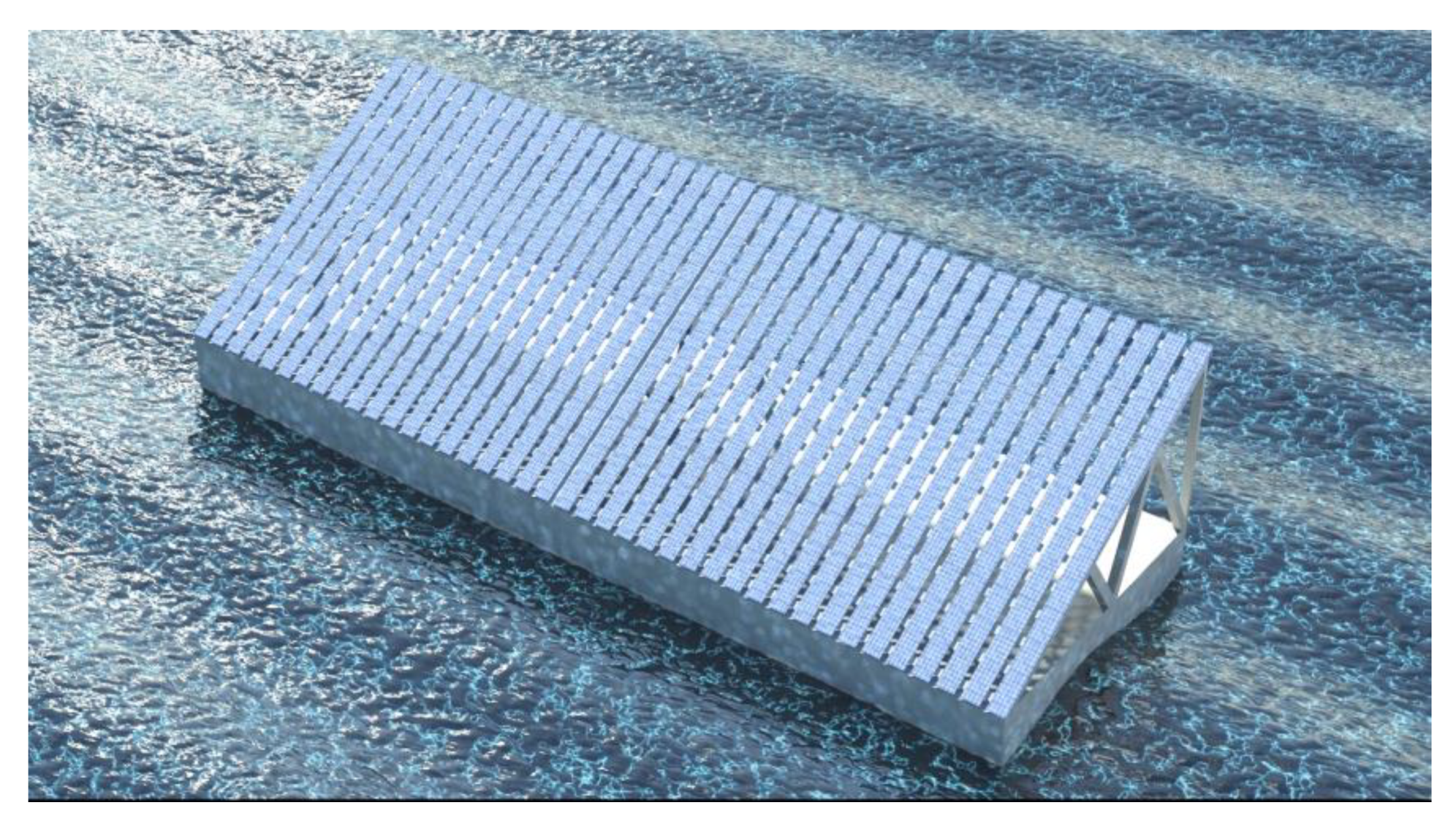
In this work, the above hydrodynamic model is extended using strip theory, to estimate the wave responses of 3D pontoon-type floating structures and their effects on the power performance in nearshore/coastal regions. The latter structure is examined as a simple alternative for the exploitation of solar energy with applications to nearshore and coastal regions of the Greek seas; see Figure 1. On the basis of linear wave theory, the wave–structure interaction problems are first solved for harmonic incident waves and subsequently the hydrodynamic response operators, calculated in the frequency domain, are used to derive the frequency spectra of the response; see, e.g., [10]. Using linear system theory, the response spectrum is exploited, in conjunction with the random phase model, to generate short-term time series of the responses of wave motions and their effects on the dynamic variation in the panel tilt angle, from which the solar power performance of the pontoon FPV is derived. Using as an example a 100 kWp floating module located in the nearshore area of the Pagasitikos Gulf and Evia Island in the central Greece region, the time series of environmental parameters concerning wave, wind and solar data are used, in conjunction with the hydrodynamic responses of the floating structure, to illustrate the effects of waves on the floating PV power performance.

In particular, we consider the FPV located in the SE coastal area of Evia Island and in the western part of the Pagasitikos Gulf, in central Greece, where a 45 m long and 15 m wide platform is considered to be deployed. Wave data were generated in the coastal regions by using the nearest offshore points from the ERA5 database in conjunction with an offshore-to-nearshore transformation technique using the SWAN wave model [11,12]. Calculated long-term responses of the FPV structure under wave loads were used to evaluate the effect on the performance of the solar station, indicating significant variations in the performance index depending on the sea state. The results were statistically processed for a typical meteorological year, and used in combination with the corresponding solar data provided by the photovoltaic geographical information system PVG_tools (https://re.jrc.ec.europa.eu/pvg_tools/en/, accessed on 24 March 2023), in order to derive predictions of the power performance of the floating module. The power output was compared against the corresponding land-based solar module configuration operating in the same nearby coastal region, and the results indicate significant variations in the energy production due to the sea environment and dynamic angle of solar incidence generated from the floating module’s responses depending on the sea state, that need to be considered in the design process. It is shown that the particular concept could be a promising and techno-economically viable alternative method concerning marine renewable exploitation contributing to the European Green Deal policies.

2. Hydrodynamic Model for Simple Floating Structures Supporting PV Modules

The hydrodynamic analysis of the floating module supporting the solar panels was performed using a BEM hydrodynamic model (see also [8]), which was based on a boundary integral formulation, involving simple singularities for the representation of the near field, in the vicinity of the floating body, in conjunction with suitable models for the treatment of radiation conditions of the considered diffraction/radiation problems. A Cartesian coordinate system x = (x₁, x₂, x₃) was used, where x₁, x₂ and x₃ are the longitudinal, transverse and vertical axes in the local coordinate system of the hull, respectively. The origin was located at the structure’s center of flotation, with the x₃-axis pointing upwards. Following linear water wave theory, the velocity field is represented by the gradient of the potential function Φ:

$$v\left(x;t\right)=\nabla \mathsf{\Phi }\left(x;t\right).$$

(1)

Under the assumptions that the free-surface elevation as well as the wave velocities are small, the potential function satisfies the linearized wave equations (see, e.g., [13]), and can be represented by

$$\mathsf{\Phi }\left(x;t\right)=\mathrm{Re}\left\{\phi \left(x;\mu \right)\cdot \exp \left(-i\omega t\right)\right\},$$

(2)

where φ denotes the complex potential function in the frequency domain, i = $\sqrt{-1}$ and μ = ω²/g is the frequency parameter, with ω being the angular frequency and g being the acceleration due to gravity.

The wave elevation is obtained in terms of the wave potential on the mean free-surface level (x₃ = 0), as follows:

$$\eta \left(x_1,x_2;t\right)=-\frac{1}{g}\frac{\partial \mathsf{\Phi }\left(x_1,x_2,0;t\right)}{\partial t}=\mathrm{Re}\left\{\frac{i\omega }{g}\phi \left(x_1,x_2,0;\mu \right)\cdot \exp \left(-i\omega t\right)\right\}.$$

(3)

A simple pontoon-type floating structure of length L is considered. The hull is characterized by a rectangular cross section of breadth B, and draft T, as schematically illustrated in Figure 1 and Figure 2. The water depth of the domain is denoted by h. The origin is located at the middle of the floating unit on the waterplane level. The hydrodynamic modeling only accounts for the roll response (ξ₄) of the structure, which dynamically alters the tilt angle of the solar panels on deck, while the linear oscillatory motions are considered not to impact the solar irradiance received. Using standard floating body hydrodynamic theory [14,15], the complex potential can be decomposed as follows:

$$\phi \left(x\right)=-i\omega {\displaystyle \sum _n{\xi }_n{\phi }_n\left(x\right)}, n=0,d,4,$$

(4)

where ${\phi }_0$ denotes the normalized incident field of unit amplitude A, φ_d is the diffracted field, ${\phi }_4$ is the radiation field induced by the angular roll oscillation of the structure about the longitudinal axis x₁, ξ₄ is the complex amplitude of the structure’s response in roll motion and ξ₀ = ξ_d = A = 1. The incident wave field is considered to be known and equal to

$${\phi }_0\left(x\right)=\frac{g}{{\omega }^2}\frac{\cosh \left(k\left(x_3+h\right)\right)}{\cosh \left(kh\right)}\exp \left(ik\left(\cos \left(\beta \right)x_1+\sin \left(\beta \right)x_2\right)\right),$$

(5)

where β denotes the direction of the incident wave propagation, as shown in Figure 2, and k is the wavenumber, calculated as the root of the dispersion relation:

$${\omega }^2=kg\tanh (kh).$$

(6)

2.1. BEM Hydrodynamic Model

Considering the elongated hull, in conjunction with the fact that the sections of the structure remain the same (orthogonal sections), and restricting ourselves to excitation mainly by waves incident from the transverse direction, a strip-theory approximation was used for the hydrodynamic analysis; see, e.g., [15]. In this context, we considered the 2D problem of incident waves to the orthogonal cross section, and the corresponding flow domain D of constant water depth h, which is enclosed by the free-surface $\partial D_{FS}$, the wetted surface of the structure $\partial D_{WS}$ and the impermeable seabed $\partial D_{BS}$; see Figure 2.

Assuming a homogeneous horizontal bathymetry profile at the vicinity of the floating structure, a mirroring technique is applied to account for the interaction of the wave field with the seabed, and the potential functions that describe the diffracted and radiated fields are represented by the following integral representation:

$${\phi }_n\left(x\right)={\displaystyle \underset{\partial D}{\int }{\sigma }_n\left(x^{\prime }\right)G\left(x^{\prime },x\right)d\ell \left(x^{\prime }\right)}, x\in D, x^{\prime }\in \partial D, n=d,4,$$

(7)

where $\partial D=\partial D_{FS}\cup \partial D_{WS}$,

$$G\left(x^{\prime },x\right)=\frac{\ln \left(\left|x^{\prime }-x\right|\cdot \left|x\prime -\widehat{x}\right|\right)}{2\pi },$$

(8)

is Green’s function for the Laplace equation in 2D, $\widehat{x}=\left(x_2,-2h-x_3\right)$ is the mirror point with respect to the bottom plane: x₃ = −h and ${\sigma }_n(x), x\in \partial D, n=d,4$ denotes the source–sink strength distribution defined on $\partial D$, corresponding to the diffraction field (n = d) and the roll radiation field (n = 4), respectively.

Based on the properties of the single-layer distributions, the corresponding derivatives of the functions ${\phi }_n(x), n=d,4$, normal to the boundary $\partial D$, are given by the following (see also [16]):

$$n\cdot \nabla {\phi }_n\left(x\right)=-\frac{{\sigma }_n\left(x\right)}{2}+{\displaystyle \underset{\partial D}{\int }{\sigma }_n\left(x^{\prime }\right)\left(n\left(x\right)\nabla G\left(x^{\prime },x\right)\right)d\ell \left(x^{\prime }\right)},\hspace{0.17em}\hspace{0.17em}\hspace{0.17em}\left(x,x^{\prime }\right)\in \partial D, n=d,4,$$

(9)

where $n\left(x\right)=\left(n_2,n_3\right)$ is the unit vector normal to $\partial D$, directed towards the exterior of the domain D.

Based on the above boundary integral representation, the diffracted and roll-radiated wave fields are evaluated by appropriately formulated boundary value problems (BVPs), involving the linearized free-surface BC (FSBC) on $\partial D_F$, as well as excitation terms on the wetted surface. Specifically, the diffracted and radiated fields are obtained as solutions of the following BVPs for $\hspace{0.17em}n=d,4$,

$${\nabla }^2{\phi }_n\left(x\right)=0,\hspace{0.17em}\hspace{0.17em}\hspace{0.17em}x\in D,$$

(10)

$$n\cdot \nabla {\phi }_n\left(x\right)-\mu (x_2){\phi }_n\left(x\right)=0, x\in \partial D_{FS},$$

(11)

$$n\cdot \nabla {\phi }_n\left(x\right)=N_n\left(x\right), \hspace{0.17em}\hspace{0.17em}x\in \partial D_{WS},$$

(12)

where

$$N_d\left(x\right)=-n\cdot \nabla {\phi }_0\left(x\right) \mathrm{and} N_4\left(x\right)=x_2{n}_3-x_3{n}_2$$

(13)

In order to eliminate the infinite extent of the domain in the x₂ direction, an absorbing layer technique was adopted, consisting of an absorbing layer which was used to attenuate the outgoing waves in an optimal way, preventing reflections from the outer boundary; see, e.g., [17]. The thickness of the layer was of the order of the local wavelength λ and the implementation of the absorbing layer was achieved by making the frequency parameter complex inside the absorbing layer, as

$$\mu (x_2)=\{\begin{array}{c}\hspace{0.17em}\hspace{0.17em}\hspace{0.17em}\hspace{0.17em}\hspace{0.17em}\hspace{0.17em}\hspace{0.17em}\hspace{0.17em}\hspace{0.17em}\hspace{0.17em}\hspace{0.17em}\hspace{0.17em}\hspace{0.17em}\hspace{0.17em}\hspace{0.17em}\hspace{0.17em}\hspace{0.17em}\hspace{0.17em}\hspace{0.17em}{\omega }^2{g}^{-1},\hspace{0.17em}\hspace{0.17em}\hspace{0.17em}\hspace{0.17em}\hspace{0.17em}\hspace{0.17em}\hspace{0.17em}\hspace{0.17em}\hspace{0.17em}\hspace{0.17em}\left|x_2\right|<R_{PML}\\ {\omega }^2{g}^{-1}{\left(1+ic\frac{{\left(\left|x_2\right|-R_{PML}\right)}^{\hspace{0.17em}q}}{{\lambda }^n}\right)}^2,\hspace{0.17em}\left|x_2\right|\ge R_{PML}\end{array}$$

(14)

In the above systems of equations, R_PML is the distance from the body where the PML is activated, and the optimized PML parameters c and q and effective length are defined depending on the angular wave frequency ω. Details concerning the values used can be found in

Table 1. Nearshore wave parameters associated with the wave climatology in the considered regions.

Nearshore Point	Hs,mean	Te,mean	Hs,std	Te,std	Hs min/max	Te min/max	R (Hs,Te)	θ,mean (deg)	θ,std (deg)
Pagasitikos Gulf	0.25 m	3.57 s	0.20 m	1.12 s	0.03/1.50 m	1.63/7.16 s	0.796	54.04	41.07
SE Evia Island	0.79 m	3.41 s	0.73 m	1.45 s	0.01/6.98 m	1.31/9.40 s	0.877	24.37	38.73

of Ref. [18].

Numerical solutions to the above BVPs were obtained by means of a low-order BEM, based on piecewise constant singularity distributions on linear 2D panels, ensuring continuity of the boundary geometry approximation; see also Belibassakis [19]. In the numerical scheme, the BCs were chosen to be satisfied at the collocation points coinciding with the panel midpoints, and therefore Equation (10) reduces to linear algebraic system(s) of M equations with M unknowns of the form $A\sigma =b$, where M denotes the number of panels used to discretize $\partial D.$ The component A_ij of the influence matrix A was calculated by the induced potential and velocity from the j–source–sink panel j to the i-collocation point and corresponds to the discretized form of the left-hand side of Equation (9), while the component b_j of the right-hand side contains the values of $N_n,n=d,4,$ given by Equation (12) and evaluated at the i-collocation point. The piecewise constant values of the source/sink strength distribution defined on the boundary $\partial D$ were then used to evaluate the potential and the velocities in the domain, as follows:

$${\phi }_n\left(x\right)={\displaystyle \sum _{m=1}^M{\sigma }_m^{(n)}}{\mathsf{\Phi }}_m\left(x\right),\hspace{0.17em}\hspace{0.17em}\hspace{0.17em}\hspace{0.17em}\nabla {\phi }_k\left(x\right)={\displaystyle \sum _{m=1}^M{\sigma }_m^{(n)}}{U}_m\left(x\right),\hspace{0.17em}\hspace{0.17em}n=d,4,$$

(15)

where ${\mathsf{\Phi }}_m(x)$ and $U_m(x)$, respectively, denote the induced potential and velocity from the m-panel with unit singularity strength to the field point, with the position vector equal to $x$, which can be calculated analytically; see, e.g., [20]. The present low-order BEM ensures very fast and accurate calculation with elimination of integration errors. The method is very cost-effective and its low computational requirements make it suitable for use in optimization problems as well.

Based on the incident, diffracted and roll-radiated wave fields, the roll response of the floating module (ξ₄) was evaluated by means of the equation of motion, as follows:

$${\xi }_4={\left[-{\omega }^2\left(I_{44}+A_{44}\right)-i\omega B_{44}+C_{44}\right]}^{-1}\left(F_{04}+F_{d4}\right)$$

(16)

where $F_{n4},\hspace{0.17em}n=0,d$ denote the Froude–Krylov (n = 0) and diffraction (n = d) roll moments, respectively. The latter were calculated via the integration of the pressure on the wetted surface induced by the incident and diffracted subfields $p_n(x)=-i\omega \rho {\phi }_n(x),\hspace{0.17em}\hspace{0.17em}n=0,d$, where ρ denotes the water density, multiplied by the component of the generalized normal vector, corresponding to rotation about the longitudinal axis,

$$F_{n4}={\omega }^2\rho {\displaystyle \underset{-L/2}{\overset{L/2}{\int }}\left[{\displaystyle \underset{\partial D_{WS}}{\int }{\phi }_n}\left(x\right)\cdot n_4\left(x\right)d\ell \left(x\right)\right]d{x}_1}={\omega }^2\rho L{\displaystyle \underset{\partial D_{WS}}{\int }{\phi }_n}\left(x\right)\cdot N_4\left(x\right)d\ell \left(x\right),\hspace{0.17em}\hspace{0.17em}\hspace{0.17em}n=0,d,$$

(17)

where in the case of the orthogonal barge, $N_4=(x_2{n}_3-x_3{n}_2)$. The added mass and hydrodynamic damping coefficients in the rolling motion of the floating pontoon were obtained from the corresponding expression of the roll–radiation moment as follows:

$${\omega }^2{A}_{44}+i\omega B_{44}=\hspace{0.17em}{\mathsf{\Pi }}_{44} \mathrm{where} {\mathsf{\Pi }}_{44}={\omega }^2\rho {\displaystyle \underset{-L/2}{\overset{L/2}{\int }}\left[{\displaystyle \underset{\partial D_{WS}}{\int }{\phi }_4}\left(x\right)\cdot N_4\left(x\right)d\ell \left(x\right)\right]d{x}_1}.$$

(18)

Finally, the moment of inertia is equal to I₄₄ = MR₄₄, where M = ρV is the mass of the structure and V = LBT is the submerged volume. The parameter C₄₄, modeling the hydrostatic restoring roll moment, equals C₄₄ = gM·GM, where GM denotes the metacentric height, evaluated as GM = KB + BM − KG, where K is the reference point at the keel of the structure, G is the center of gravity, B denotes the center of buoyancy located at x₃ = −T/2, and the metacentric radius BM is evaluated as BM = I/ρ∇, where I is the second moment of area of the waterplane along the longitudinal axis x₁, which in the case of the floating pontoon is given by Ι = LB³/12.

2.2. Numerical Results and Hydrodynamic Model Verification

Results obtained via the numerical scheme described above were compared against experimental measured data from the literature for verification purposes. The results concern a pontoon-type structure floating at depth h, with dimension ratios L/h = 3, B/h = 1 and T/h = 0.2, and the radius of gyration about the longitudinal axis is R₄₄ = 0.4B. 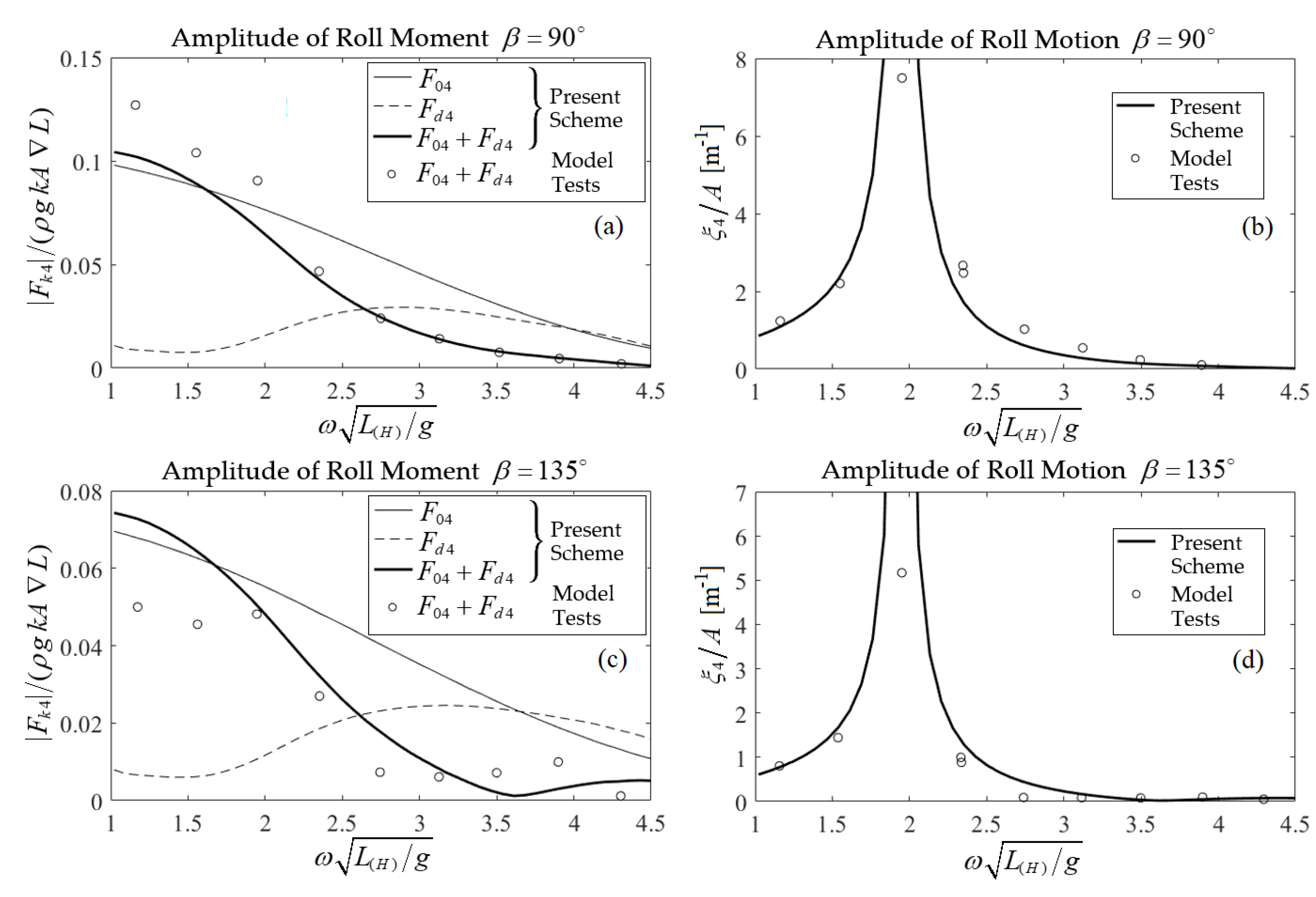Numerical and experimental results regarding the above configuration have been presented by Pinkster and van Oortmerssen [21]. In the latter work, model tests were carried out in the shallow water laboratory of the Netherlands Ship Model Basin, which measures 210 m in length and 15.75 m in breadth, and the water depth is equal to 1 m. The tests were carried out using a model at a scale of 1:50. Regular waves were generated at one end of the basin via a flap-type wave maker, while a perforated sloping beach at the other end of the basin served as a wave damper to minimize reflections. Concerning the present discrete BEM model, a minimum of 20 boundary elements per wavelength was applied to the free-surface boundary, while the number of equally distributed panels on the wetted surface of the pontoon cross section was 300, which was found to be sufficient for numerical convergence.

Figure 3a depicts the normalized Froude–Krylov, diffraction and total roll moments acting on the wetted surface, as calculated by the present BEM scheme and as measured by the model tests [21] for beam seas, with incident waves propagating at β = 90°. The Froude–Krylov, diffraction and total roll moments, as calculated by the present BEM scheme, were also plotted using thin, dashed and thick lines, respectively. Figure 3b shows the resulting response in roll motion for beam seas (β = 90°), as calculated via the present numerical scheme using Equation (13), and as measured using model tests. The corresponding results for quartering waves (β = 135°) are presented in Figure 3d. It can be seen that the present model is able to provide numerical predictions in good agreement with the experimental data.

Using the calculated responses of the above floating structure, for incident waves characterized by frequency spectra, in conjunction with many year-long time-series of wave parameters for the nearshore region where the structure is considered, the effect of waves on the power performance of the FPV system was estimated and comparatively presented against a nearby land-based solar park with the same components and dimensions. The above result was obtained by considering the dynamic variation in the angle of incidence of the solar irradiance on the FPV configuration, taking into account the perturbation of the tilt angle of the panels due to the structure wave responses; see also [8]. As an example, two nearshore/coastal sites in the Greek sea region were considered for the deployment and operation of the pontoon-type FPV structure, as described in the sequel.

3. Offshore-to-Nearshore Transformation of Wave Conditions

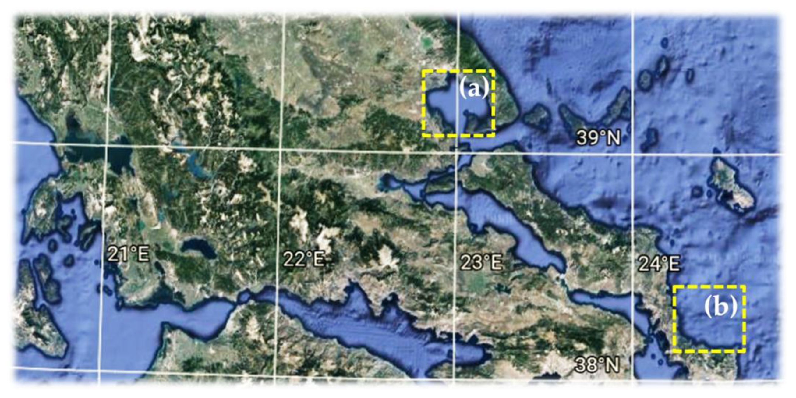
The nearshore/coastal regions of western Pagasitikos Gulf in central Greece, and SE coastal area of Evia Island, shown in Figure 4, are considered to demonstrate the applicability of the present method regarding the evaluation of the floating solar module’s power performance. In the above regions, a simple pontoon-type platform with dimensions L = 45 m in length and B = 15 m in breadth is considered to be deployed, in salt water of depth h = 15 m. The water density is ρ = 1025 kgr/m³ and the draft of the structure is T = 3 m, and therefore the total mass of the FPV is M = 2.075 × 10⁶ kg and the roll moment of inertia is I₄₄ = 7.47 × 10⁷ kgm². Moreover, the center of gravity is assumed to be located at a vertical distance of 3 m above the keel.

As described in more detail in the sequel, an offshore-to-nearshore transformation technique was used to generate wave data in the coastal location of the floating structure, based on corresponding offshore wave and wind data, in conjunction with geographical information, in order to account for the effects of the wave-induced dynamic motions on the power output of the FPV.

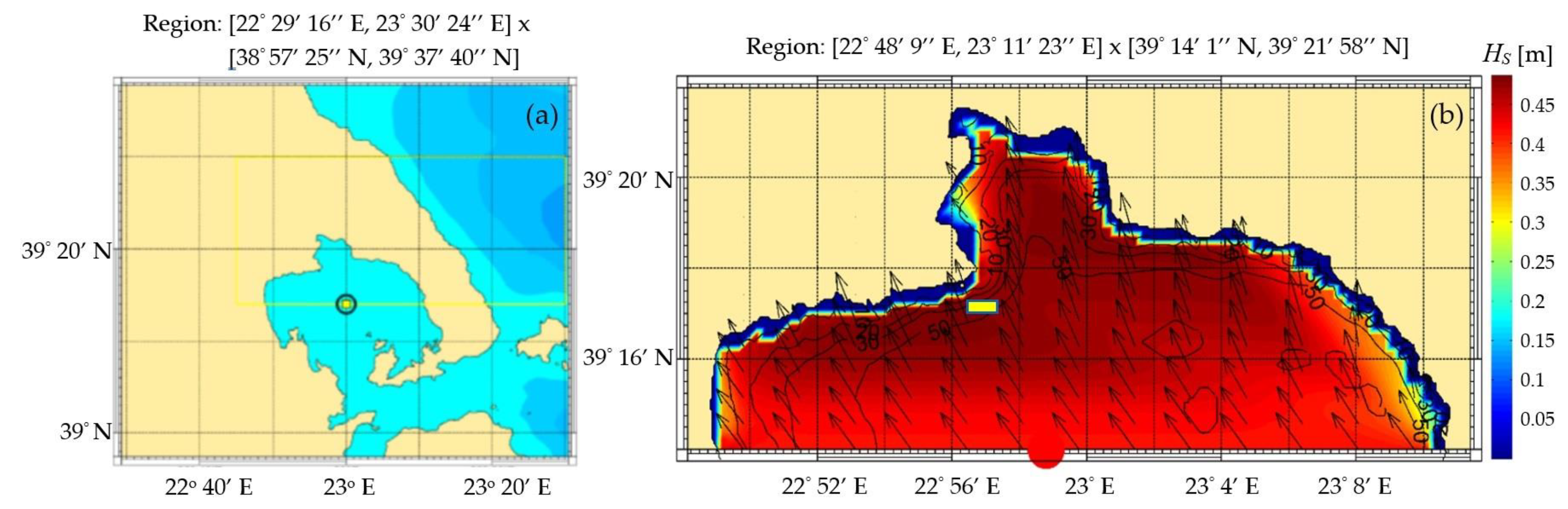
Several sources of offshore wave and wind data are available regarding the sea area of interest. The most complete databases come from the application of wave models that are operationally run at meteorological and oceanographic centers and from dedicated long-term hindcasts which have been performed. Moreover, satellite data with good spatial coverage are available in offshore areas around the globe. In order to obtain the nearshore wave conditions, the transformation of offshore data was used. This was achieved by using nearshore wave models for the transformation of waves using offshore wind and wave data, in conjunction with bathymetric and coastline data in the region under study. 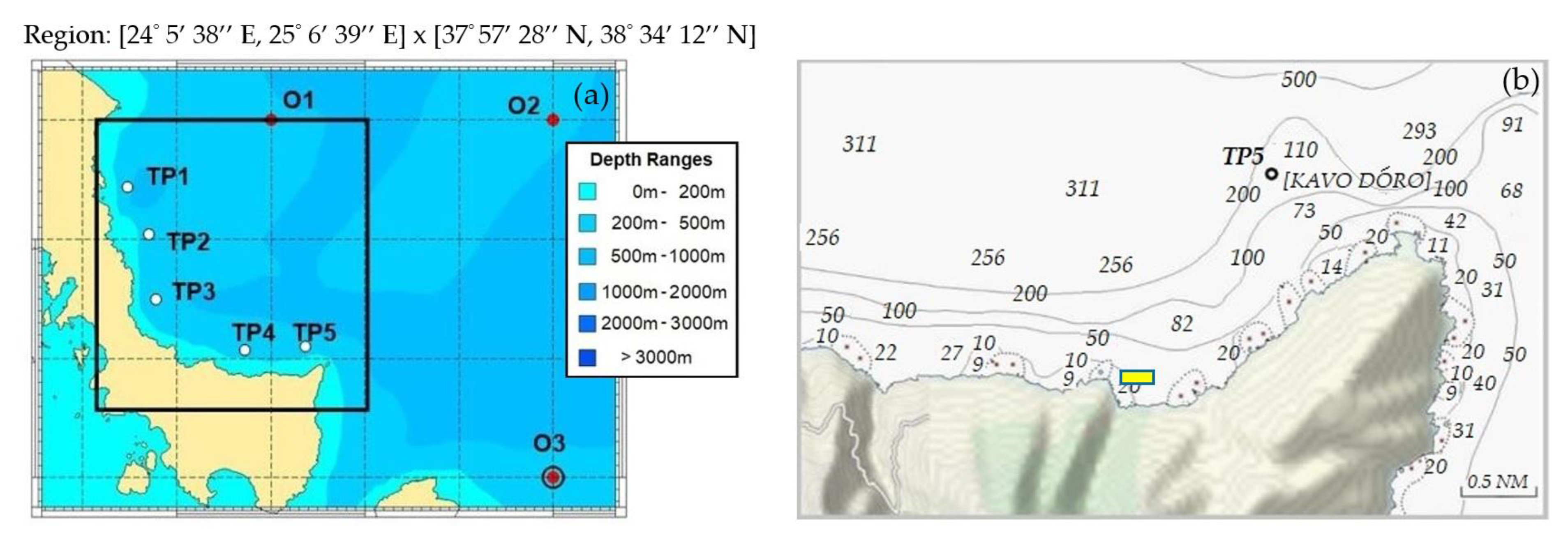Concerning the Pagasitikos Gulf region, the geographical area considered was [22°48′9′′ E, 23°11′23′′ E]–[39°14′1′′ N, 39°21′58′′ N], shown in Figure 5. In the SE coastal area of Evia Island, the geographical area considered was defined by the coordinates [24°10′ E, 24°40′ E]–[38°05′ N, 38°30′ N], shown in Figure 6. In both cases, the floating pontoon was considered to be deployed with the longitudinal axis directed to the east).

In the present work, the wave climate in the considered nearshore regions was derived from the ERA database of offshore-to-nearshore (OtN) transformation of wave conditions, obtained by means of the SWAN wave model [11,12]. The bathymetric data in the area of interest were used together with coastline data in order to set up the SWAN model for calculating the offshore-to-nearshore wave transformation for the nearshore target point coinciding with the location of the FPV, at water depth h = 15 m. The bathymetric data used in the SWAN wave model for the OtN transformation of wave conditions in the extended region were created via the combination of the EMODnet Digital Bathymetry (DTM 2016) which is based on more than 7700 bathymetric data sets from various countries near European Seas and is provided on a grid resolution of 1/8 by 1/8 arc minute of longitude and latitude [22]. The database used for the coastline was the Global, Self-Consistent, Hierarchical, High-Resolution Shoreline Database (GMT—GSHHS) provided under the GNU Lesser General Public License; see Wessel and Smith [23]. 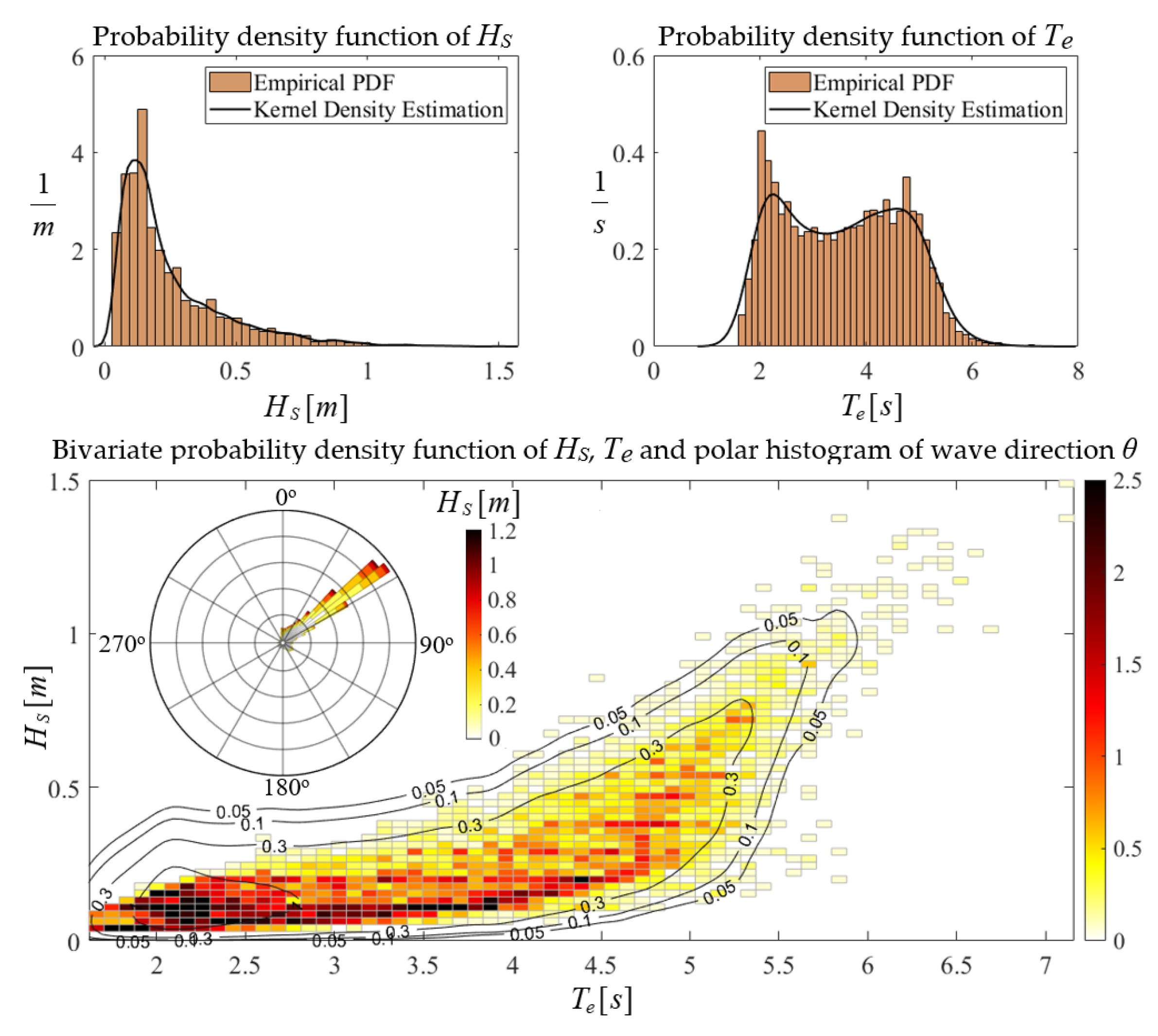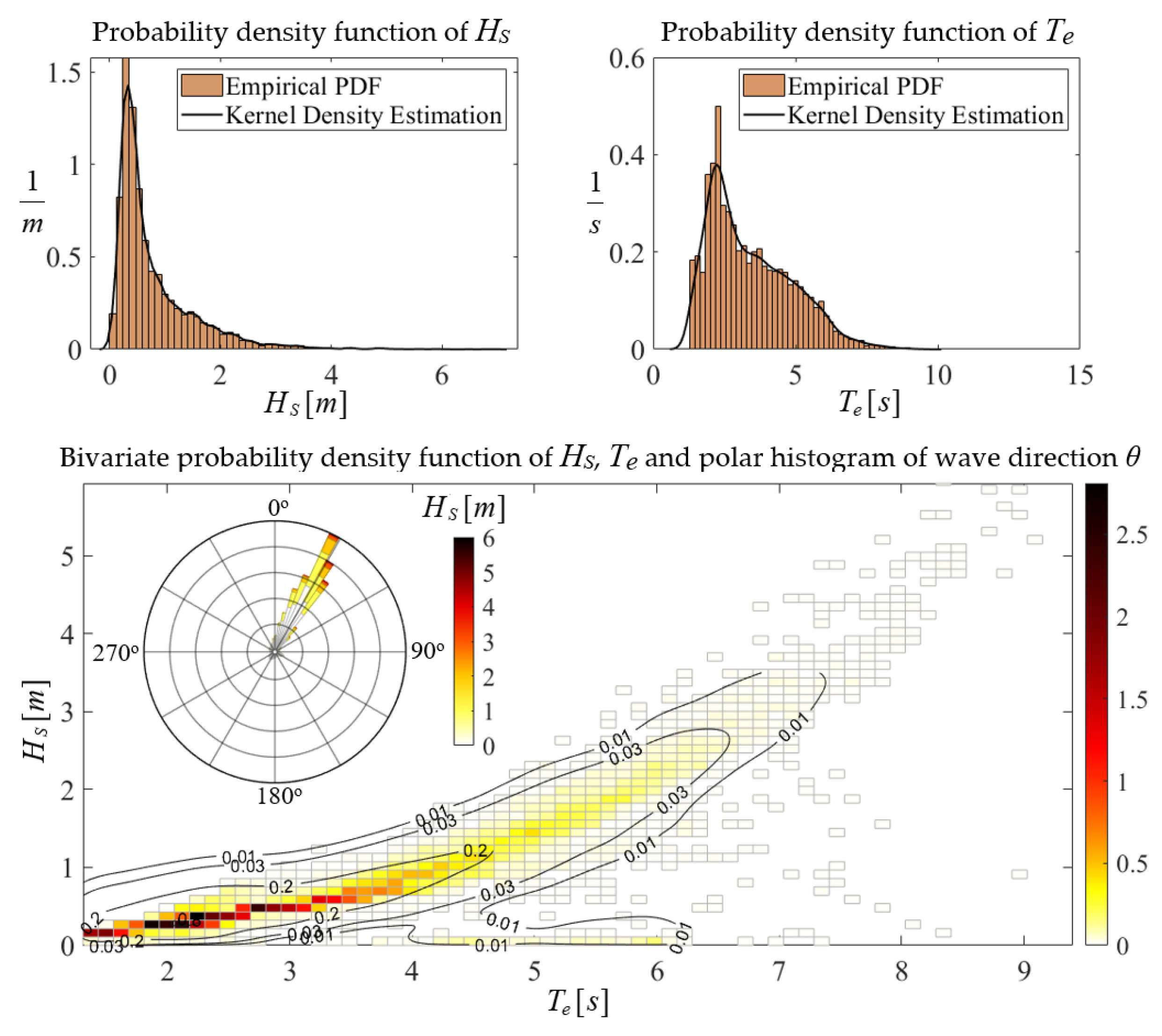The OtN methodology is described in more detail in [24], and the derived wave climatology in the two nearshore regions considered is presented in Figure 7 and Figure 8, respectively. Moreover, the basic statistical measures concerning wave characteristics (i.e., significant wave height H_s, mean energy period T_e and mean wave direction θ_m) at the two considered locations, including standard deviation and minimum (min) and maximum (max) values, are comparatively presented in Table 1.

4. Responses of the FPV Structure

The nearshore time series of wave parameters are used to define the corresponding incident wave spectra using the JONSWAP model, as presented in Figure 9a for a representative case. The latter model is defined by

$$S\left(f|H_S,T_{-10}\right)=\left(\frac{a{g}^2}{{\left(2\pi \right)}^4{f}^{\hspace{0.17em}5}}\exp \left[-1.25{\left(\frac{f}{f_p}\right)}^{-4}\right]{\gamma }^{\delta \left(f\right)}\right),$$

(19)

where $f=\omega /2\pi$ is the linear frequency and ω is the angular frequency; $f_p=1/T_p$ is the peak frequency estimated as $f_p=0.906/T_e$, and g = 9.81 m/s² is the acceleration due to gravity. Also, $a$ is a normalization parameter suitably defined such that $H_s^{}=\hspace{0.17em}4\sqrt{m_0^{}}$, where $m_0^{}$ is the zeroth-order spectral moment. Finally, the parameter $\gamma$ and the function $\delta \left(f\right)$ are defined as follows:

$$\gamma =3.3, \mathrm{and} \delta =\exp \left[-\frac{{\left(f-f_p^{}\right)}^2}{2{\sigma }_0^2{f}_p^2}\right] \mathrm{with} {\sigma }_0=\{\begin{array}{c}0.07,\hspace{0.17em}\hspace{0.17em}\hspace{0.17em}\hspace{0.17em}\hspace{0.17em}\hspace{0.17em}\mathrm{for}\hspace{0.17em}\hspace{0.17em}\hspace{0.17em}f<f_p\\ 0.09,\hspace{0.17em}\hspace{0.17em}\hspace{0.17em}\hspace{0.17em}\hspace{0.17em}\hspace{0.17em}\mathrm{for}\hspace{0.17em}\hspace{0.17em}\hspace{0.17em}f\ge f_p\end{array}$$

(20)

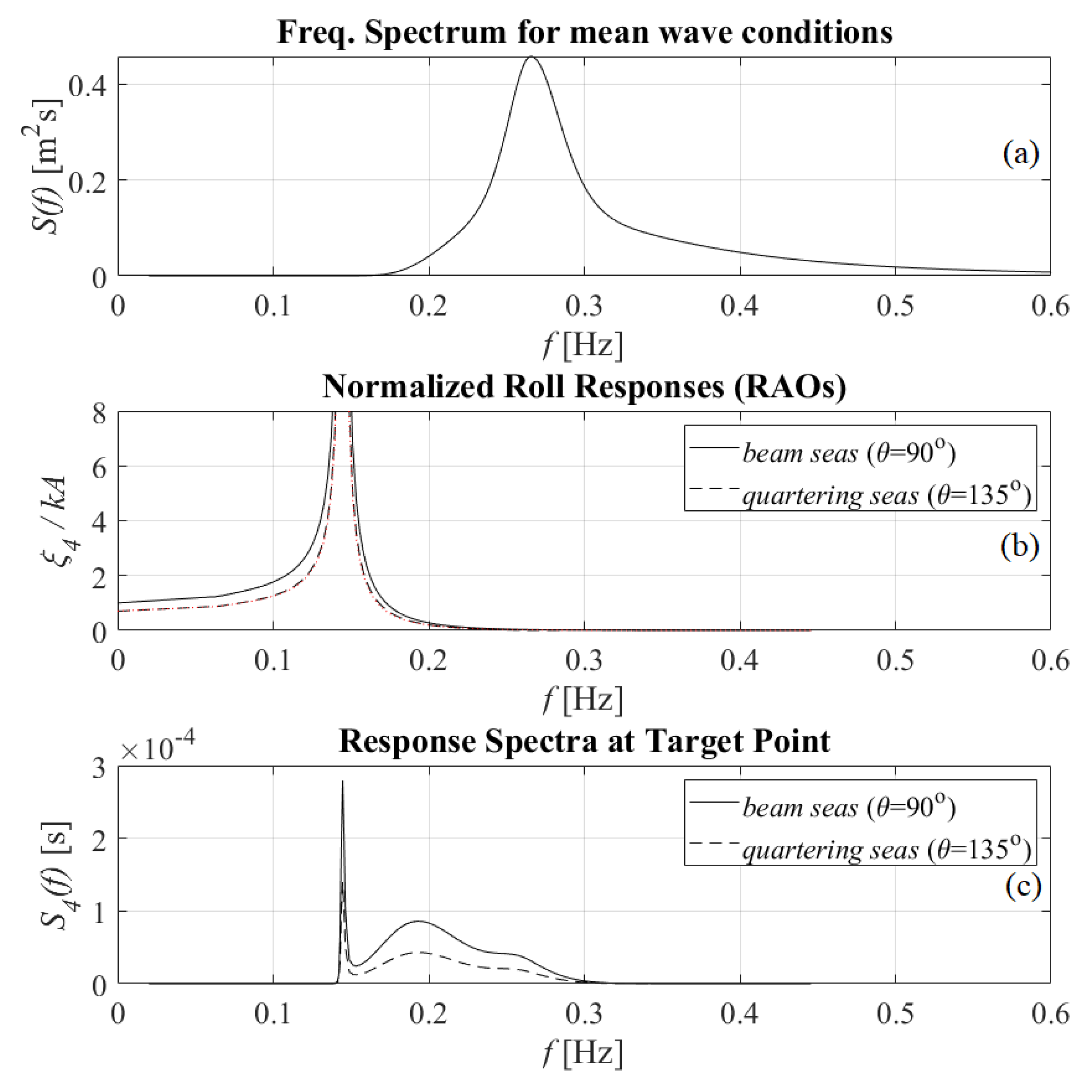
In order to combine the wave with the solar data in the considered region of the FPV and evaluate the power output performance, time series for a typical meteorological year were derived by taking mean values for each 6 h interval point in the long-term time series of wave parameters and each date of the year. The derived wave data were used to reconstruct nearshore frequency spectra and were combined with the roll response functions (RAO) of the considered pontoon structure, as presented in Figure 7 for two wave incident angles (β = 90° for beam waves, and β = 135° for beam-quartering seas) to obtain the spectra characterizing the rolling motion of the FPV.

In the example presented in Figure 9, we consider the FPV located in the coastal area of Evia Island (see Figure 6) and the incident wave spectra corresponding to the climatological mean value at the point, whereby significant wave height is H_s = 0.79 m and the corresponding value of the mean energy period T_e = 3.41 s. In this case, the frequency spectrum using the JONSWAP model shown in Figure 9a is combined with the roll response (RAO) of the FPV plotted in Figure 9b, and we derived the roll motion spectra as shown in Figure 9c for two incident angles (β = 90° for beam waves, and β = 135° for quartering seas).

For simplicity, we considered unidirectional incident waves, and the roll response spectrum was calculated using the RAO of the roll motion of the structure, as follows:

$$S_4\left(\omega \right)={\displaystyle \underset{\theta =0}{\overset{2\pi }{\int }}RA{O}^2\left(\omega ,\beta =\theta -{\psi }_H\right)k^{2}S\left(\omega \right)}d\theta ,$$

(21)

where $S\left(\omega \right)=S\left(f\right)/\left(2\pi \right)$, θ is the mean wave direction in geographical space and the wavenumber k is evaluated using the dispersion relation, Equation (6), for each frequency of water waves at water depth h = 15 m at the considered location. Moreover, ${\psi }_H$ denotes the angle of the longitudinal axis of the structure with respect to the east, measured from east to south, and in the considered example, ψ_H = 0° and thus β = θ.

Using the fact that the cross sections of the FPV are the same in the fore-aft direction, in conjunction with the transverse symmetry of the FPV structure, in the present work the pontoon FPV roll response, for various incident wave directions, is approximated by the following relation:

$$RAO\left(\omega ,\theta -{\psi }_H\right)\approx RA{O}_{2D}\left(\omega ,\beta \right)\left|\cos \left(\theta -{\psi }_H\right)\right|,$$

(22)

where $RA{O}_{2D}\left(\omega ,\beta \right)$ denotes the sectional response of the pontoon structure, which was obtained from Equation (16) for various frequencies of incident waves.

Based on the calculated roll response spectrum $S_4\left(\omega \right)$, simulated time series of roll motion ${\xi }_4\left(t;H_s,T_e,\theta \right)$ of the structure were constructed, for the considered configuration (structure and coastal environment), for each data point in the time series of incident waves characterized by the parameters $H_s,\hspace{0.17em}\hspace{0.17em}{T}_e$ and $\theta$. These were obtained using the random phase model, see, e.g., Refs. [10,25]. The response time series of the structure under spectral excitation was approximated by the following representation:

$${\xi }_4\left(t\right)={\displaystyle \sum _{n=1}^{{\rm N}}{A}_n}\cos \left(-{\omega }_n\hspace{0.17em}t+{\epsilon }_n\right), \mathrm{where} A_n=\sqrt{2S_4\left({\omega }_n\right)\mathsf{\Delta }{\omega }_n}$$

(23)

where ${\epsilon }_n\in \left[0,2\pi \right)$ are random phases.

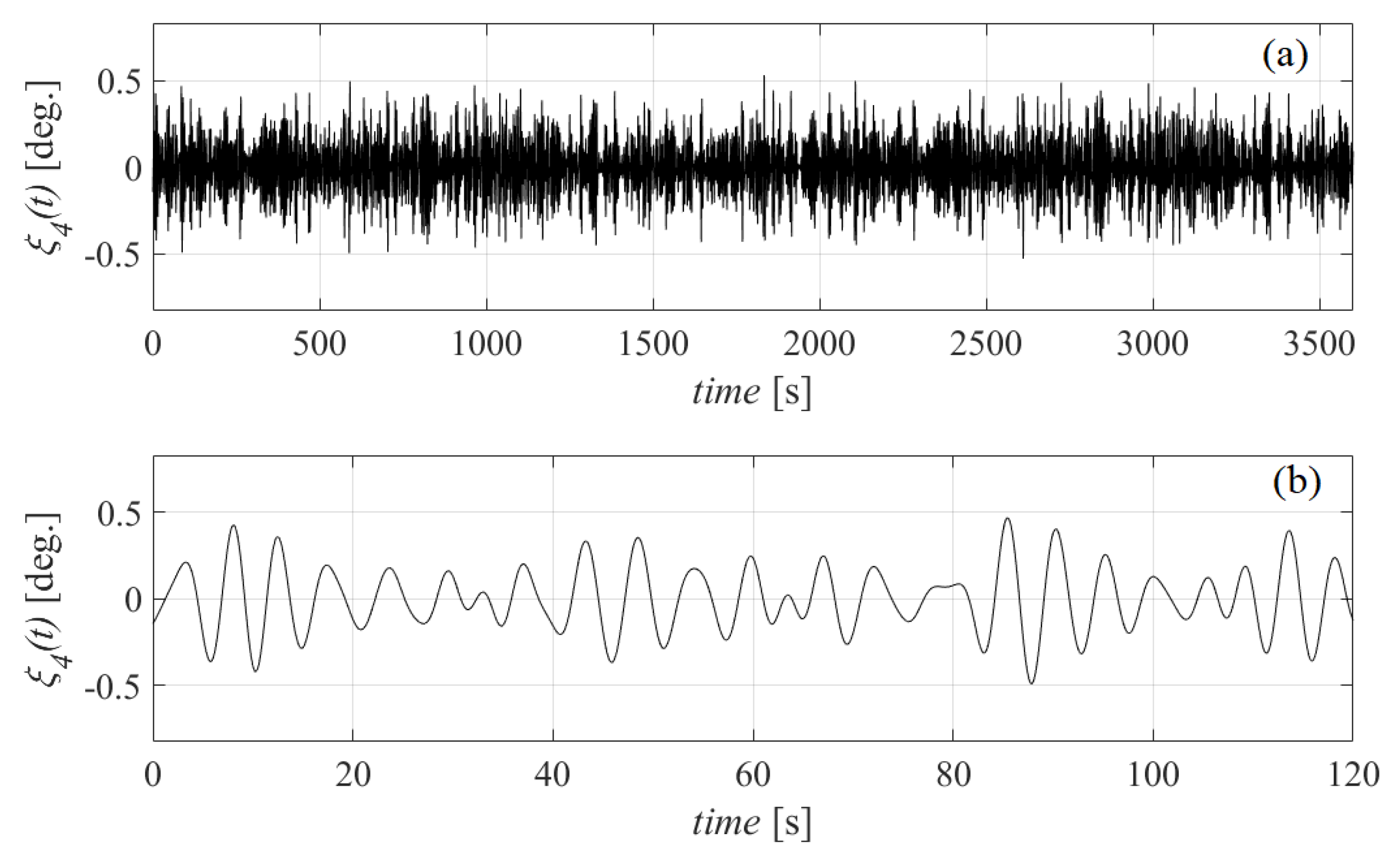
An example of roll motion simulated time series of the considered pontoon FPV structure, in the case of quartering incident waves with significant wave height equal to H_s = 0.79 m, peak period T_e = 3.41 s and mean direction θ_m = 24.37° (corresponding to the climatological mean values at the FPV coastal location of the SE Evia Island region), is presented in Figure 10. In the sequel, the short-time roll responses ${\xi }_4\left(t;H_s,T_e,{\theta }_m\right)$ for each wave condition were used to calculate the angle of incidence (AOI) at the FPV and the resulting effect on the power output performance of a PV system, in conjunction with other data concerning the tilt (with respect to the deck of the structure) and their orientation (azimuth angle), as described in the following section.

5. Effects of Waves on FPV Module Power Performance

The power performance of a floating photovoltaic (FPV) unit is based on a variety of factors, many of which result from the local marine environment. While certain factors that influence the energy efficiency of FPV are also found in corresponding land-based units, with comparable power output levels, others are not present in land installations. In the sea, there is generally a higher level of humidity than inland, as well as lower ambient temperatures. Several factors contribute to the temperature drop, including the transparency of water, which leads incoming solar radiation to exceed the surface layer and be transmitted to the inner layers of the medium, as well as the fraction of incident irradiation that is used for evaporation. Furthermore, wind speed is typically higher than on land due to longer fetch distances. The above parameters contribute to maintaining a lower operating temperature of the solar cells, which in turn leads to increased efficiency. In this work, in order to proceed to a preliminary calculation of the power output of the considered FPV module including the effect of the rolling motion due to excitation from waves, the following equation was used:

$$P\left(t\right)={\eta }_{pv}{A}_{pv}G\left(1-k_p\left(T_c-T_{stc}\right)\right),\hspace{0.17em}\hspace{0.17em}\hspace{0.17em}\hspace{0.17em}\hspace{0.17em}\hspace{0.17em}\mathrm{where}\hspace{0.17em}\hspace{0.17em}\hspace{0.17em}\hspace{0.17em}\hspace{0.17em}G=B+D+R.$$

(24)

In Equation (24), P is the power generated by the solar panels, ${\eta }_{pv}$ is the efficiency of the panels based on standard temperature conditions (STCs), $A_{pv}$ is the panel surface area, G is the global irradiance on the panels, $k_p$ is the temperature coefficient, $T_c$ is the cell’s temperature in a specific time and $T_{STC}$ is the standard test temperature.

For the examined configuration concerning the FPV platform of length 45 m and total breadth 15 m, a 100 kWp arrangement is considered, consisting of 11 parallel strings of 40 in-series modules (see Figure 1). In order to estimate the data, the Sanyo HIP-225HDE1 panel modules of 225 Wp nominal power, with dimensions 1.6 m × 0.86 m, V_PM = 33.9 V and I_PM = 33.9 V, were considered, with module efficiency of 15% at T_STC = 25 °C. Thus, the total panel area of panels on the FPV structure was A = 605.44 m² and k_p ≈ 0.4%/°C was used as an approximate value for the silicon panel technology. The total radiation G received by the panels consisted of the direct (beam) radiation B and the diffuse horizontal irradiation D, and it also included the reflected irradiance component R. The latter components were calculated as follows (see, e.g., [26]):

$$B=DNI\left({\ell }_1+{\ell }_2\cos \left(HRA\right)+{\ell }_3\sin \left(HRA\right)\right),$$

(25)

where

$${\ell }_1=\sin \left(\delta \right)\sin \left(\phi \right)\cos \left({\beta }_p\right)-\sin \left(\delta \right)\cos \left(\phi \right)\cos \left({\beta }_p\right),$$

(26)

$${\ell }_2=\cos \left(\delta \right)\cos \left(\phi \right)\cos \left({\beta }_p\right)+\cos \left(\delta \right)\sin \left(\phi \right)\sin \left({\beta }_p\right)\cos \left(\psi \right),$$

(27)

$${\ell }_3=\cos \left(\delta \right)\sin \left(\psi \right)\sin \left({\beta }_p\right),$$

(28)

and

$$D=DHI\left(\pi -{\beta }_p\right)/\pi ,$$

(29)

where DNI is the direct normal irradiance on a plane always normal to sun rays and DHI is the diffuse horizontal irradiance. In the above equations, δ is Earth’s declination angle, φ is the latitude of the location, ψ is the module azimuth measured from south to west and ${\beta }_p$ is the module tilt. Moreover, HRA is the hour angle defined by means of the local solar time. Regarding the case study presented in this work, the FPV latitude ranged from φ = 38.5° to 39.5° N, and the azimuth was selected to be ψ = 0°, describing a configuration with solar panels facing towards the south, which is close to the optimal value. The tilt with respect to the horizontal deck in still water was set to β = 30° and the HRA was defined in terms of the longitude and the equation of time (EOT); see, e.g., [26]. More importantly, the PV performance was directly affected by the angle of incidence (AOI) of solar irradiation, which in the case of FPV installations was influenced by the wave-induced responses. To account for the above effect, noting that the structure was oriented with its longitudinal axis directed to the east (see Figure 5 and Figure 6), the tilt angle of the present FPV panel configuration in the above equations was replaced by the corresponding dynamic value obtained by the summation of the static value and the instant roll response of the FPV defined on the short time scale, as described in the previous section, for each sea state in the constructed time series of the TMY.

$${\beta }_{FPV}\left(t\right)={\beta }_p+{\xi }_4\left(t\right).$$

(30)

In the general case, all angular responses of the floating structure contribute to the dynamic perturbation of the panel tilt angle ${\beta }_{FPV}\left(t\right)$, and future work will be directed to this extension, requiring the hydrodynamic analysis of the floating structure in 6 dof. Concerning the reflected irradiance component R, it is approximated in the present work as

$$R\left(t\right)=c\hspace{0.17em}(B+D),$$

(31)

where the coefficient c takes into account the albedo effect, which for the water body is taken approximately as c = 0.1, as compared to the albedo of a nearby rural area, taking values c = 0.2–0.4.

Data concerning the direct normal irradiance (DNI), diffuse horizontal irradiance (DHI) and environmental conditions concerning the cell temperature and wind for the specific site were obtained from the PVGIS SARAH2 database in the form of a typical meteorological year (TMY) data set for the specific site with a 1 h temporal resolution, provided by PVG tools (https://re.jrc.ec.europa.eu/pvg_tools/en/, accessed on 24 March 2023). The latter data set provides information concerning the dry-bulb temperature and relative humidity, from which the ambient temperature is calculated by the following (see also [27]):

$$T_A=T_{DB}+0.33p_V-0.7U-4,$$

(32)

where $T_A$ is the apparent temperature, $T_{DB}$ is the dry-bulb temperature at 2 m height, $U$ is the wind speed and $p_V$ is the vapor pressure in hPa, which is calculated using the following equation:

$$p_V=\exp \left(1.8096+17.69D/\left(273.3+D\right)\right).$$

(33)

In the above equations, D is the dew point temperature and it is estimated based on the relative humidity RH, using the approximate formula $D=100-0.2\left(100-RH\right)$ that is valid for RH > 50% (which is expected near the sea). The values of RH included in the TMY data set are used for calculations regarding the land-based configuration, while at sea it is assumed that RH = 80% (see https://www.gfdl.noaa.gov/blog_held/47-relative-humidity-over-the-oceans/, accessed on 24 March 2023).

After calculating the ambient temperature, the panel cell temperature was estimated using the following correlation provided by Sandia National Laboratories:

$$T_C=G\exp \left(a+bU\right)+T_A,$$

(34)

where G is the solar irradiance incident on the panels, and a and b are parameters depending on the module construction, which for glass/cell/polymer sheet panels are defined as $a=-3.56,\hspace{0.17em}\hspace{0.17em}b=-0.075$; see [28].

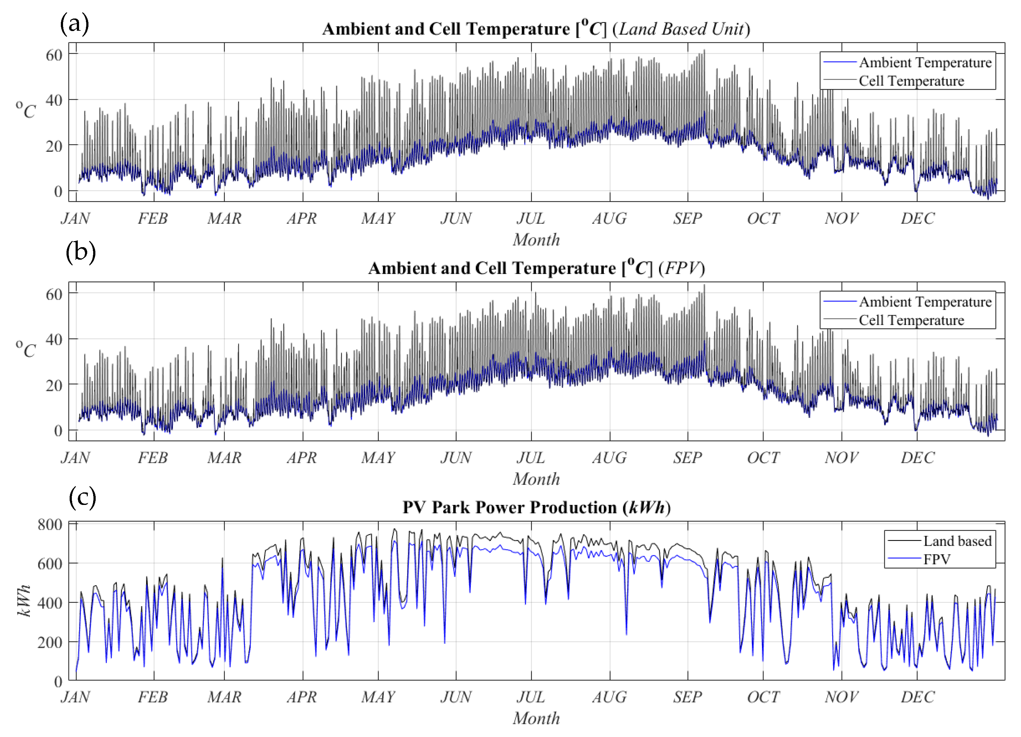
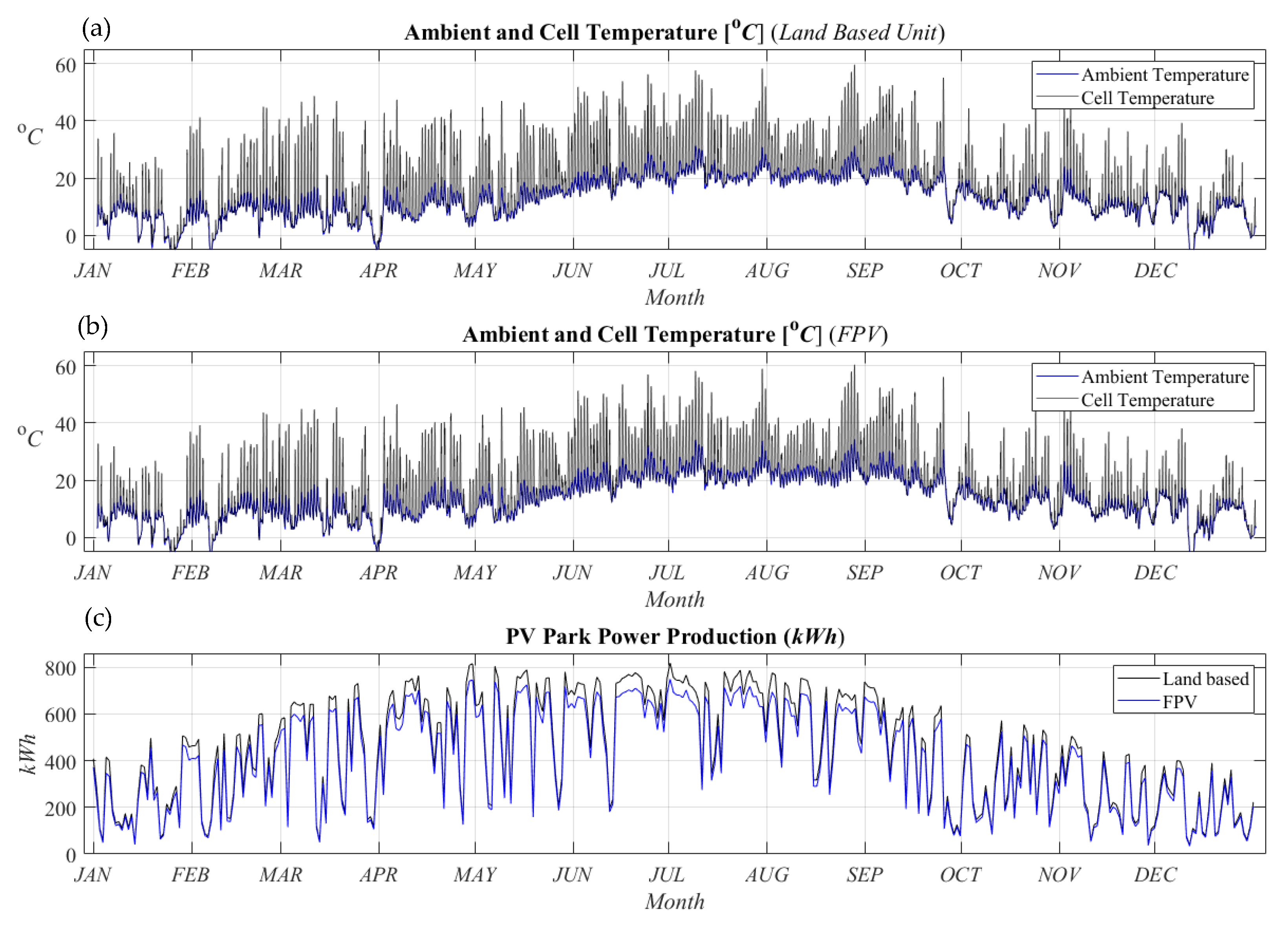
The numerical results concerning the performance and energy production of the considered 100 kWp system are presented comparatively in Figure 11 and Figure 12 for a land-based module and the considered FPV configuration located at the geographical nearshore/coastal locations of Pagasitikos Gulf and the SE region of Evia Island, respectively. In particular, the ambient and cell temperatures of the land-based and the floating configurations are presented in the subplots (a, b) of each figure, respectively, and the daily energy production in a TMY is shown in subplot (c). In the latter plots, the results concerning the calculated daily energy production for a fixed (inland) nearby configuration and for the FPV system in a TMY are comparatively plotted, using black and blue lines, respectively. It is observed that the dynamic variation in the angle of attack on the panels produced by the wave loads, along with the effect of the albedo of seawater, leads to a drop in the energy production, which is more pronounced in the summer period due to the additional adverse effect of the cell temperature. In the examples considered in this work, the calculated annual production drops by about 8–9%, from 173.5 MWh (nearby inland configuration) to 159.3 MWh (FPV) in the Pagasitikos Gulf and from 164.4 MWh (inland configuration) to 150.3 MWh in the SE region of Evia Island, respectively.

It is worth mentioning here that the water surface acts as an imperfect reflector that affects the panels’ temperature. In addition, water vapor above the water surface absorbs part of the near-infrared radiation that is most effective for photovoltaic energy conversion in crystalline silicon-based PV panels, which is an adverse effect. On the contrary, the presence of water, in conjunction with airflow due to wind, contributes to cooling. Additionally, a salty and humid sea environment constitutes an important additional parameter concerning the degradation of PV panels in the sea environment (see, e.g., [29]). Moreover, the improvement in the performance of the system by means of the cleaning of the solar panels due to rainfall and other parameters could be taken into account. The study of the above effects necessitates additional modeling and data and will be considered in future work.

Furthermore, electric system losses have not been taken into account and will be included in future extensions of the present model, that will also take into account the effects of all angular responses of the floating structure and the general orientation of the structure and panels on the angle of incidence. Finally, future research will be focused on the estimation of wind effects both concerning the cooling of the panels and concerning the strength and stability of the arrangement on the deck, as well as the stress of various structural parts, including cables and connectors.

6. Conclusions

The increased availability of solar energy potential, especially in southern latitudes such as the Mediterranean and the Greek Sea regions, constitutes a strong motivation for the design and development of floating offshore solar energy platforms suitable for deployment and operation in the marine environment. In this work, a BEM was used for the hydrodynamic analysis of floating-pontoon-type structures carrying photovoltaic panels on deck. The method supports the investigation of wave responses and their effects on solar power performance. A boundary integral formulation, involving simple singularities, was applied in the vicinity of the floating body for the representation of the near field, while a mirroring technique was applied to account for the interaction of the wavefields with the seabed, in conjunction with suitable models for the treatment of radiation conditions of the considered diffraction/radiation problems. Using as an example a 100 kWp module located in western Pagasitikos Gulf and the SE region of Evia Island, the effects of waves on the floating PV performance are presented, indicating significant variations in energy production due to dynamic variation in the angle of solar incidence generated from the floating module roll responses depending on the marine environment and the sea state. Future extensions of the method include the consideration of electric system losses and the cooling and cleaning effects of panels due to rainfall, as well as the effects of 6 dof motion on the FPV hydrodynamic responses due to waves. Finally, the wind effects on the cooling of the panels and on the stability of the panel arrangement on deck will be addressed.