
Application of the XBeach-Gravel Model for the Case of East Adriatic Sea-Wave Conditions

Abstract
:1. Introduction
2. Materials and Methods
2.1. GWK Data Set and Numerical Model Setup (Laboratory Conditions)
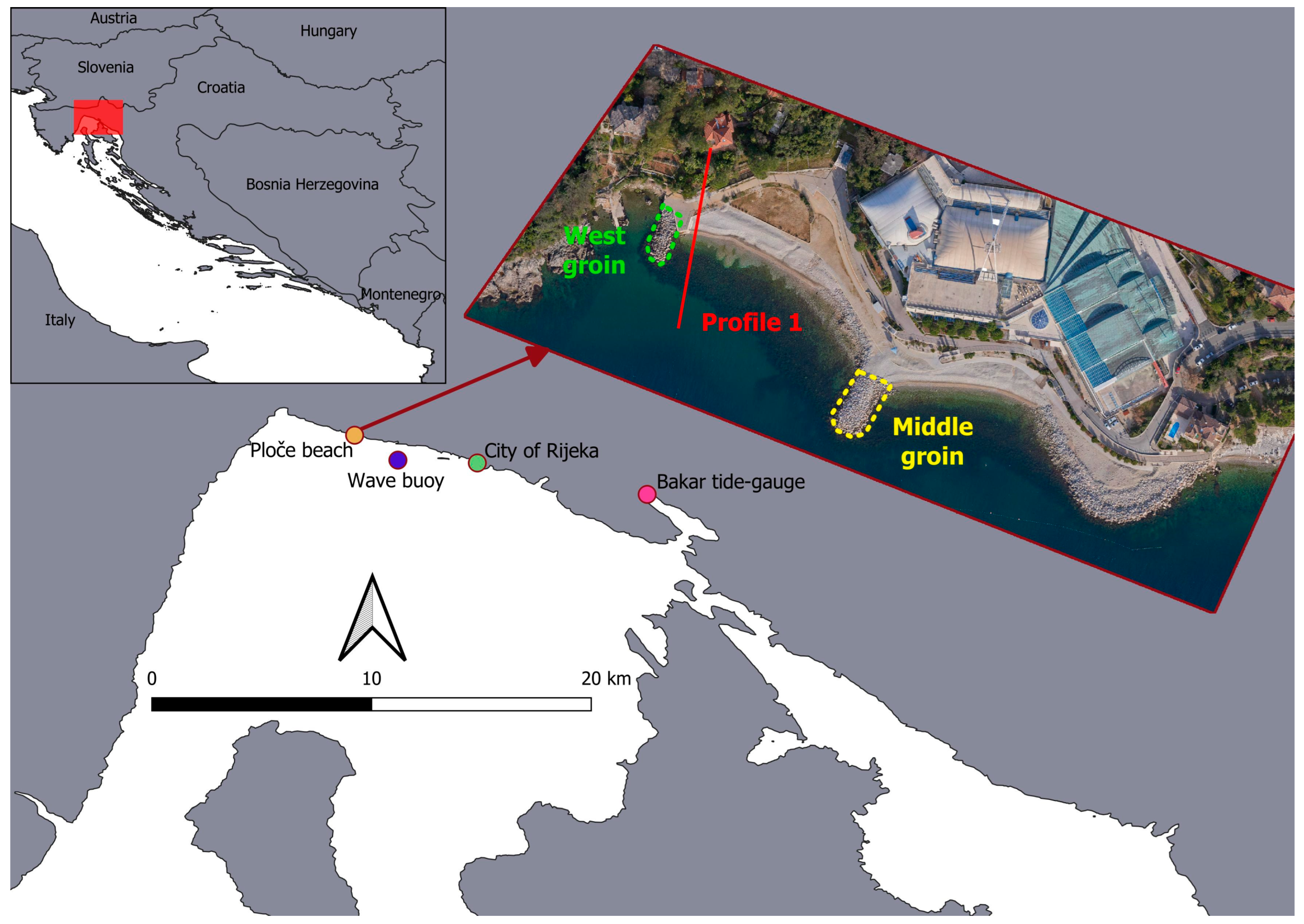
2.2. Ploče Beach Data Set and Numerical Model Setup (Field Conditions)
2.3. Brier Skill Score
3. Results
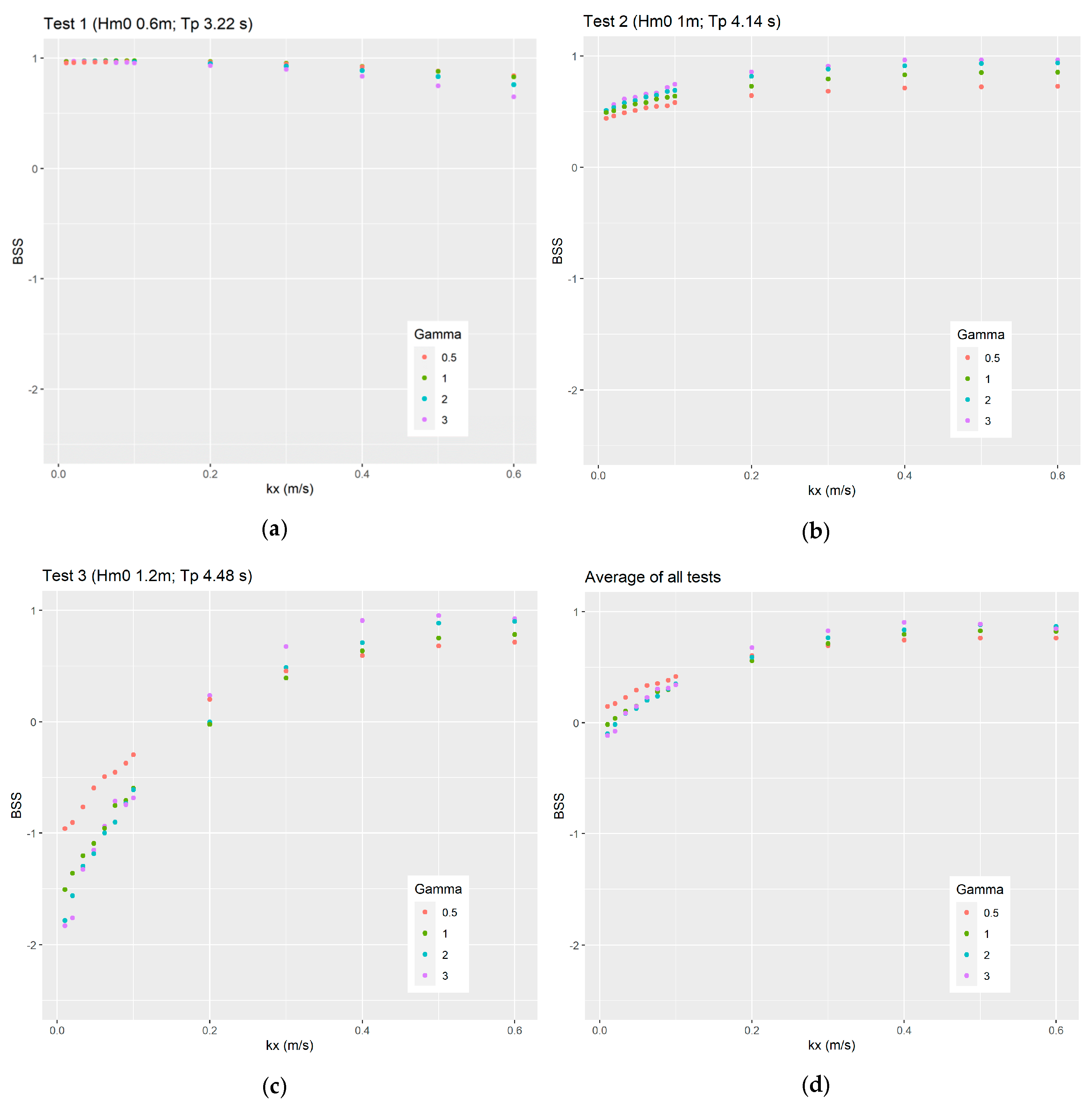
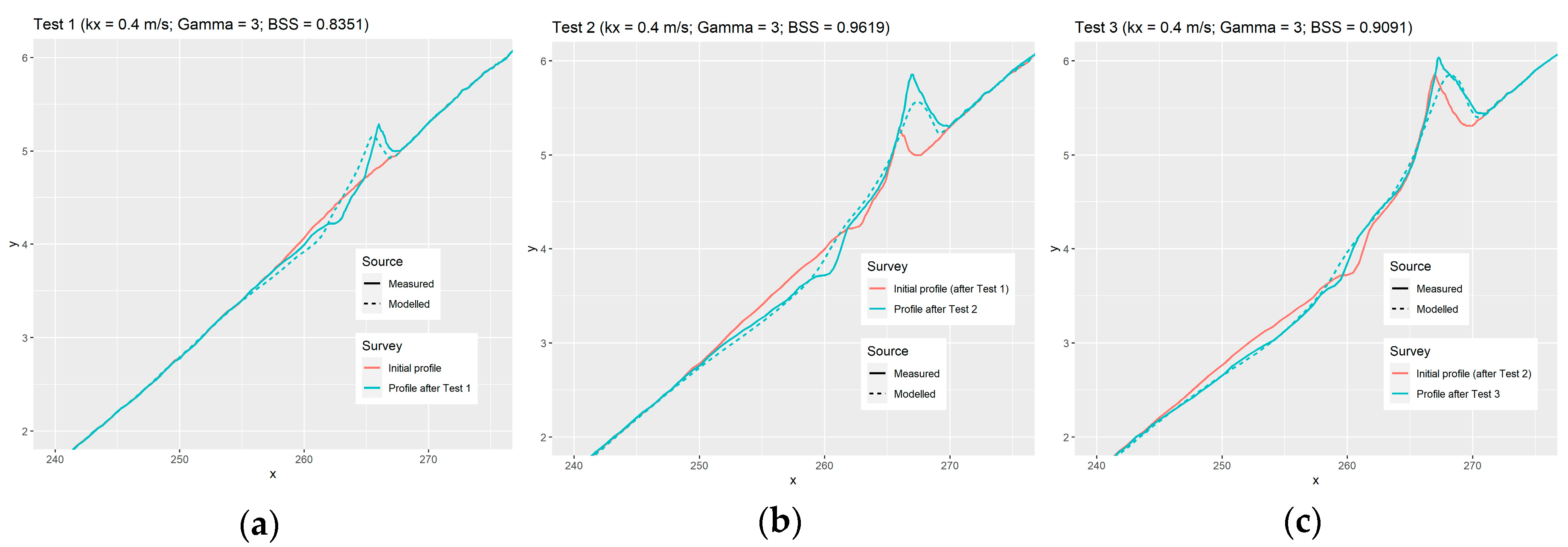
3.1. XBeach-Gravel Calibration for the GWK Data Set (Laboratory Conditions)
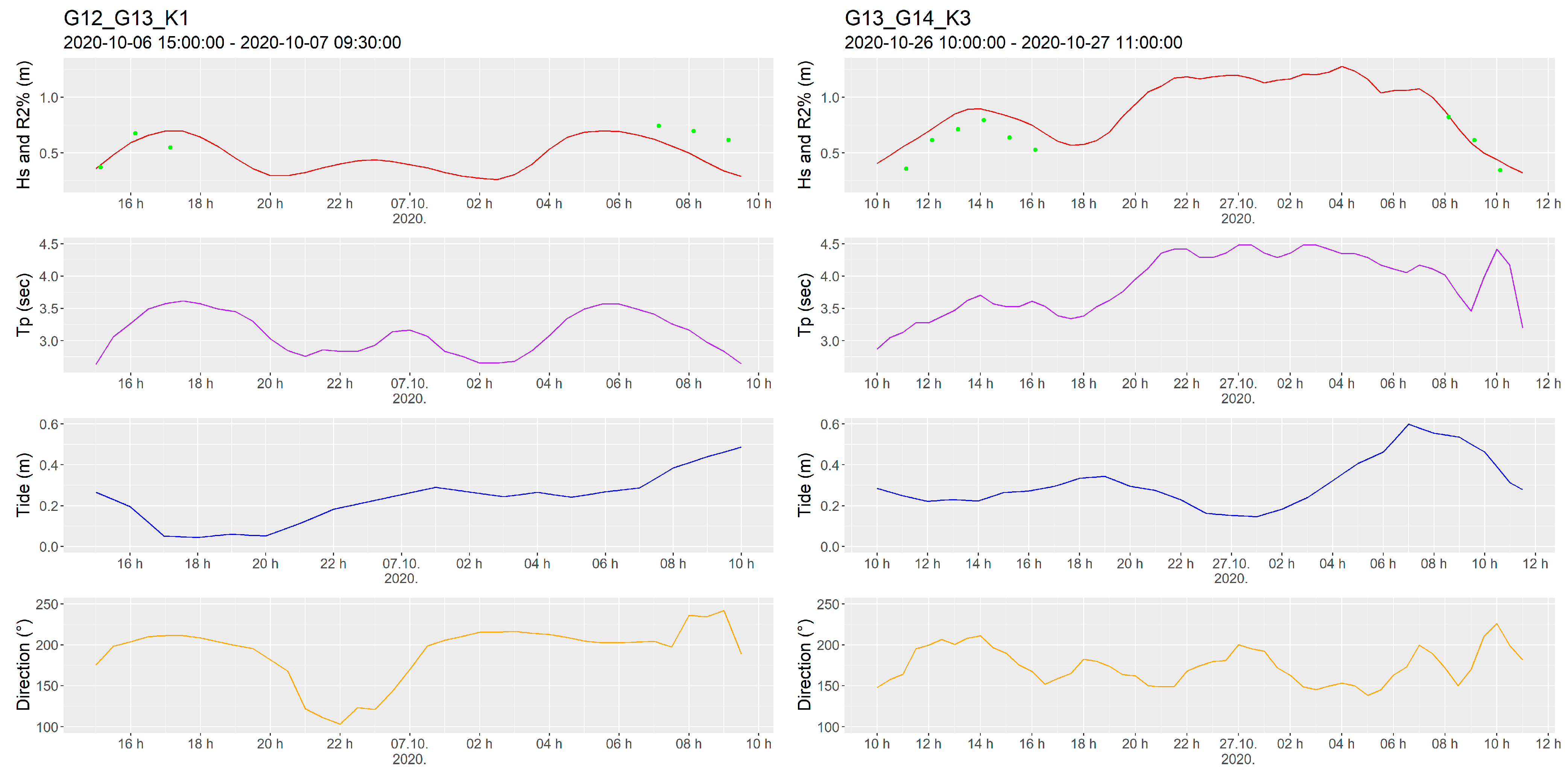
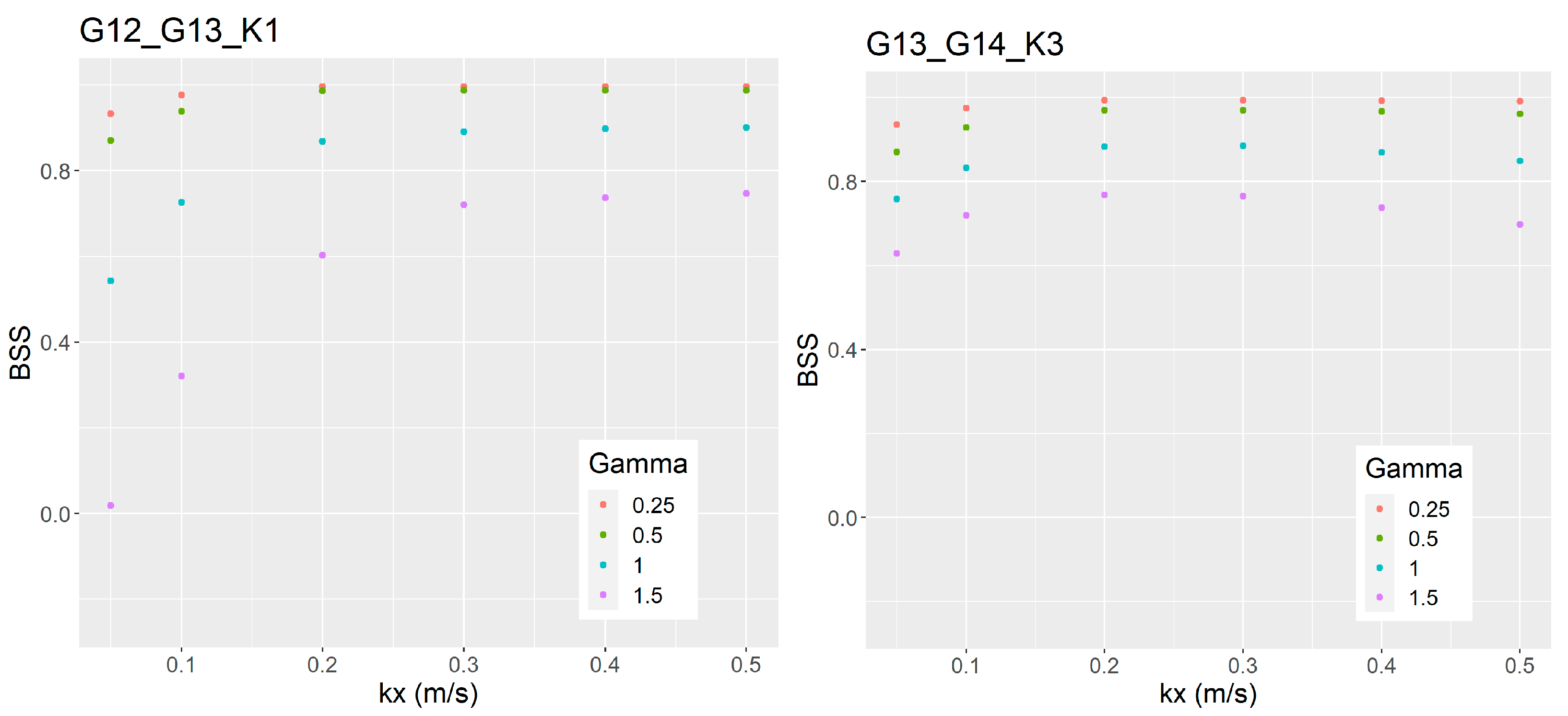
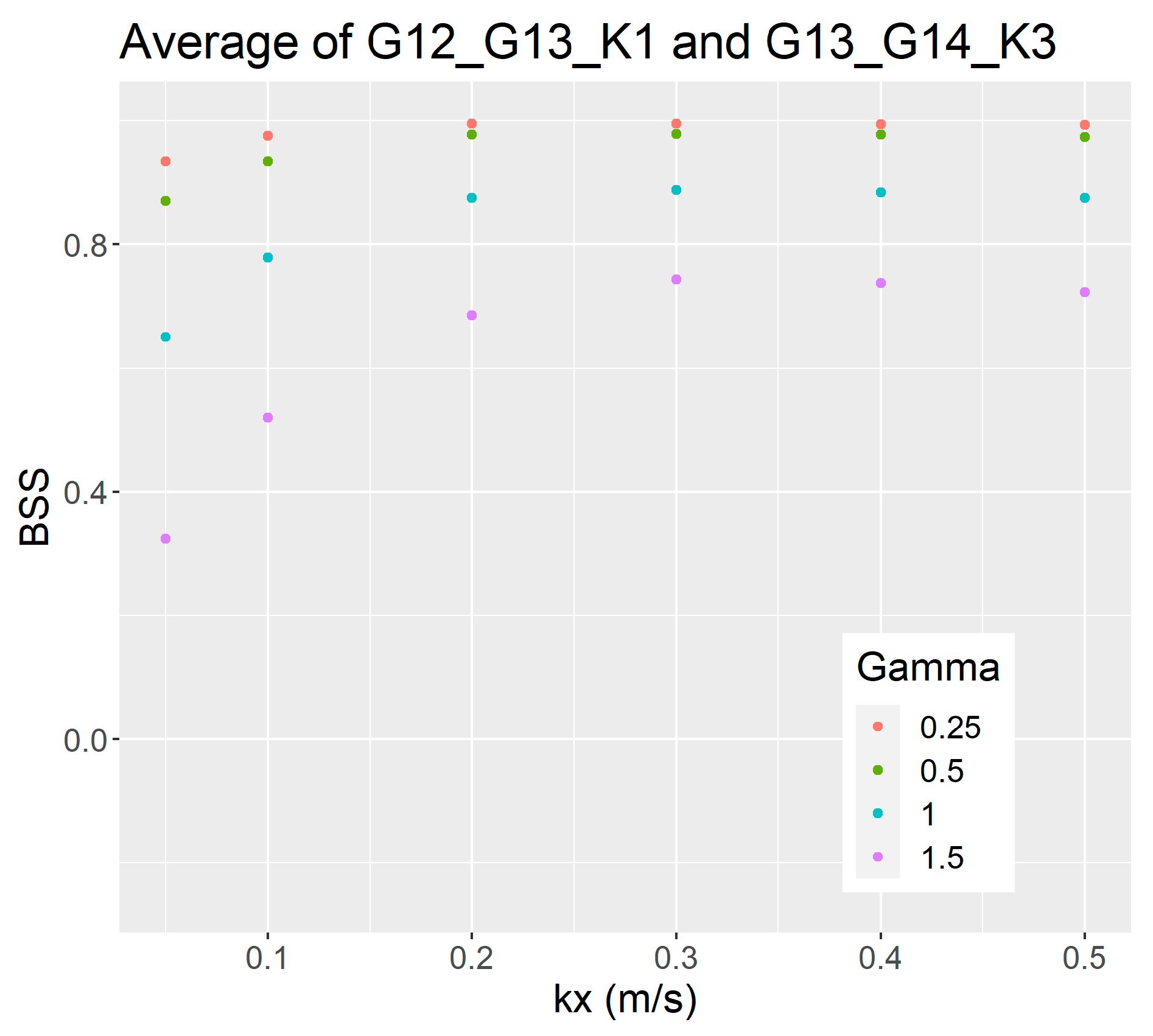
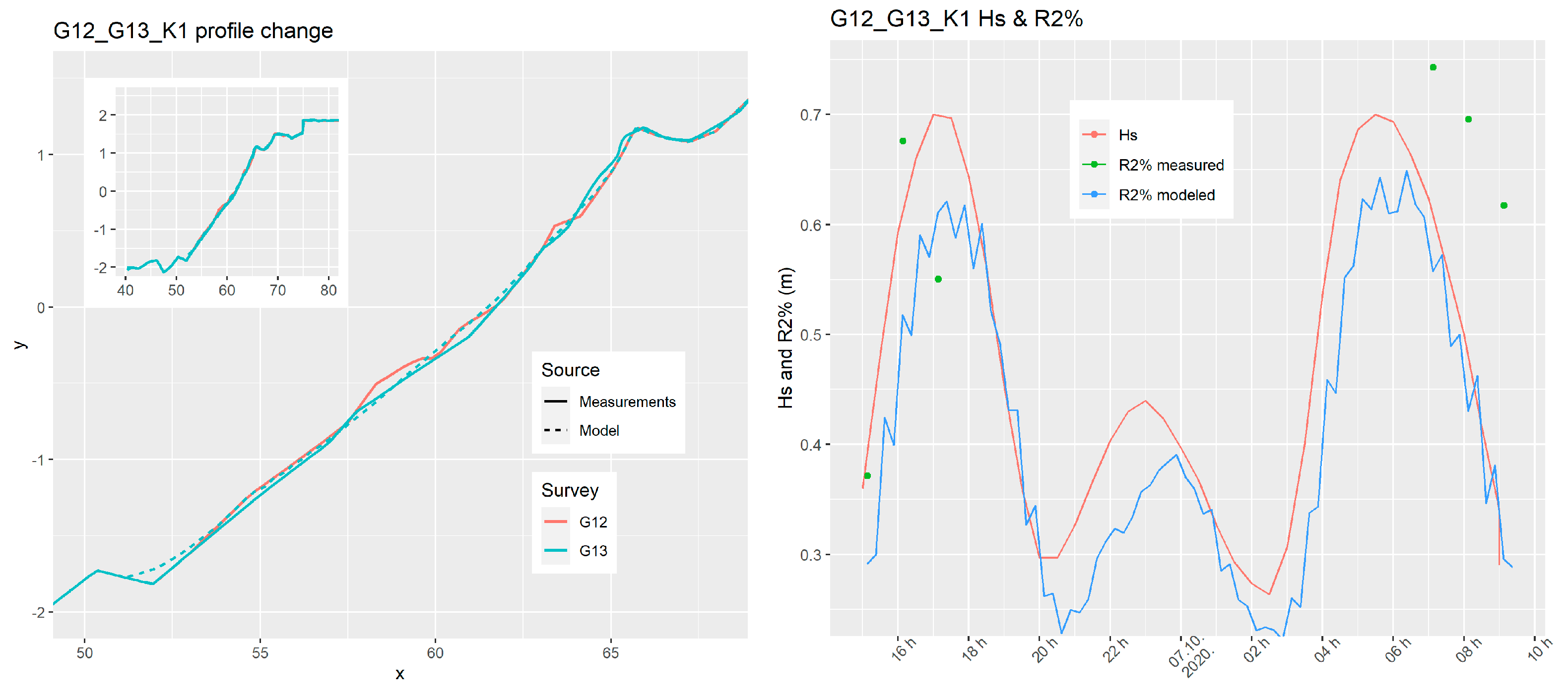
3.2. XBeach-Gravel Calibration for the Ploče Data Set (Field Conditions)
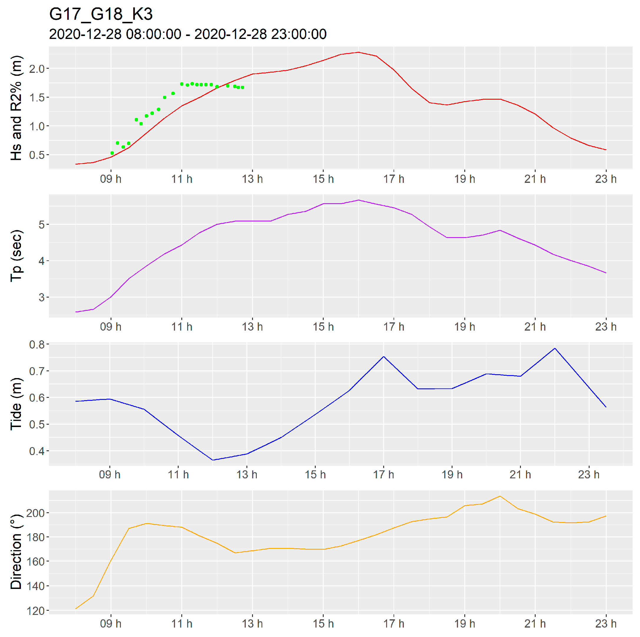
3.3. Validation for the Case of Wave Overtopping
4. Discussion
Author Contributions
Funding
Institutional Review Board Statement
Informed Consent Statement
Data Availability Statement
Acknowledgments
Conflicts of Interest
Appendix A

| Parameter Name | GWK—Test 1, 2 and 3 | Beach Ploče—G12_G13_K1 and G13_G14_K3 | Beach Ploče—G17_G18_K3 | ||
|---|---|---|---|---|---|
| Profile parameter setup | |||||
| Minimum grid size (m) | 0.1 | 0.1 | 0.1 | ||
| Maximum grid size (m) | 1 | 0.5 | 0.5 | ||
| Minimum points per wavelength | 40 | 60 | 60 | ||
| Maximum offshore bottom level (m) | 0 | −2 (m) for both simulations | −4 (m) | ||
| Coordinates | Constructed profile of Beach I in the GWK and subsequent profiles after Test 1, 2, and 3 | Geodetic survey 12 and 13, respectively | Geodetic survey 17 | ||
| Wave parameters setup | |||||
| Spectrum type | Unimodal for all waves | Unimodal for all waves | Unimodal for all waves | ||
| Gamma | 3.3 for all waves | 3.3 for all waves | 3.3 for all waves | ||
| Significant wave height (m) | Test 1 | Test 2 | Test 3 | 30 min average of Hs provided by the buoy measurements for each storm, smoothed by 1.5 h rolling average | 30 min average of Hs provided by the buoy measurements for each storm, smoothed by 1.5 h rolling average |
| 0.6 | 1 | 1.2 | |||
| Peak period (s) | Test 1 | Test 2 | Test 3 | 30 min average of Tp provided by the buoy measurements for each storm, smoothed by 1.5 h rolling average | 30 min average of Tp provided by the buoy measurements for each storm, smoothed by 1.5 h rolling average |
| 3.22 | 4.14 | 4.48 | |||
| Spreading | 10 for all waves | 30 min average of S provided by the buoy measurements for each storm, smoothed by 1.5 h rolling average | 30 min average of S provided by the buoy measurements for each storm, smoothed by 1.5 h rolling average | ||
| Tide parameters setup | |||||
| Back boundary water level | Variable | Variable | Variable | ||
| Offshore water level (m) | Set to 4.7 m for the entire simulation | 30 min interpolated data from the 1 h tide-gauge measurements at Bakar for each storm | 30 min interpolated data from the 1 h tide-gauge measurements at Bakar for each storm | ||
| Parameters setup | |||||
| Duration (s) | Test 1 | Test 2 | Test 3 | 68,400/91,800 | 55,800 |
| 8400 | 7200 | 7800 | |||
| Initial groundwater level (m) | 0 | 0 | 0 | ||
| Bottom aquifer (m) | 0 | 0 | 0 | ||
| D50—Median grain size (m) | 0.021 | 0.02 | 0.02 | ||
| Hydraulic conductivity (m/s) | 0.01, 0.02, 0.034, 0.048, 0.062, 0.076, 0.09, 0.1, 0.2, 0.3, 0.4, 0.5 | 0.05, 0.1, 0.2, 0.3, 0.4, 0.5 | 0.3 | ||
| Angle of repose (°) | 35 | 35 | 35 | ||
| Sediment transport formula | Van Rijn | Van Rijn | Van Rijn | ||
| Inertia coefficient (Ci) | 1 | 1 | 1 | ||
| Transport coefficient (γ) | 0.5, 1, 2, 3 | 0.25, 0.5, 1, 1.5 | 0.25 | ||
Appendix B

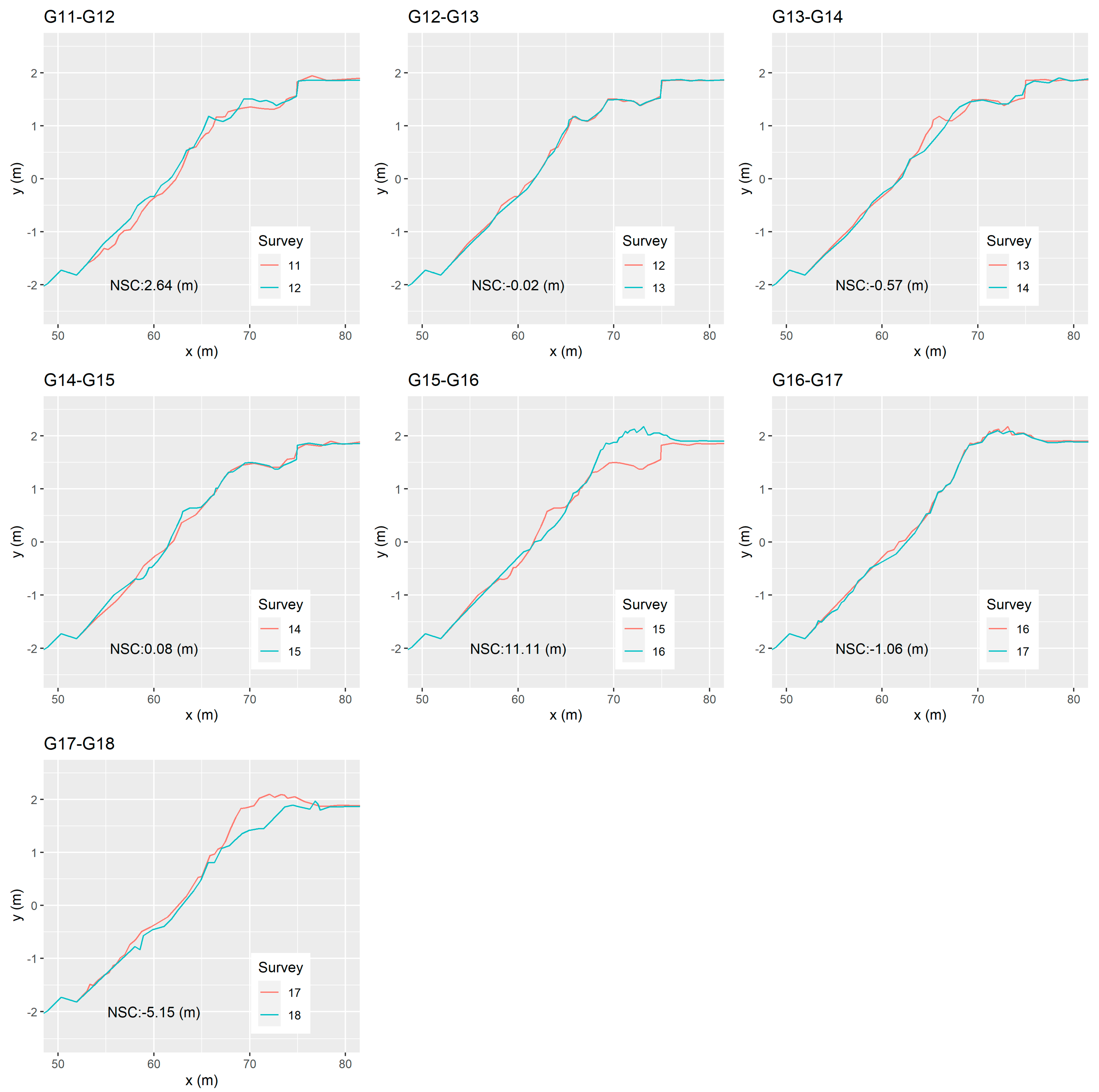
| Geodetic Surveys | Number of Wave Events | Net Sediment Change (m) | Start of Event | End of Event | Hs Max (m) | Average Wave Direction (°) | Runup Measurement | |
|---|---|---|---|---|---|---|---|---|
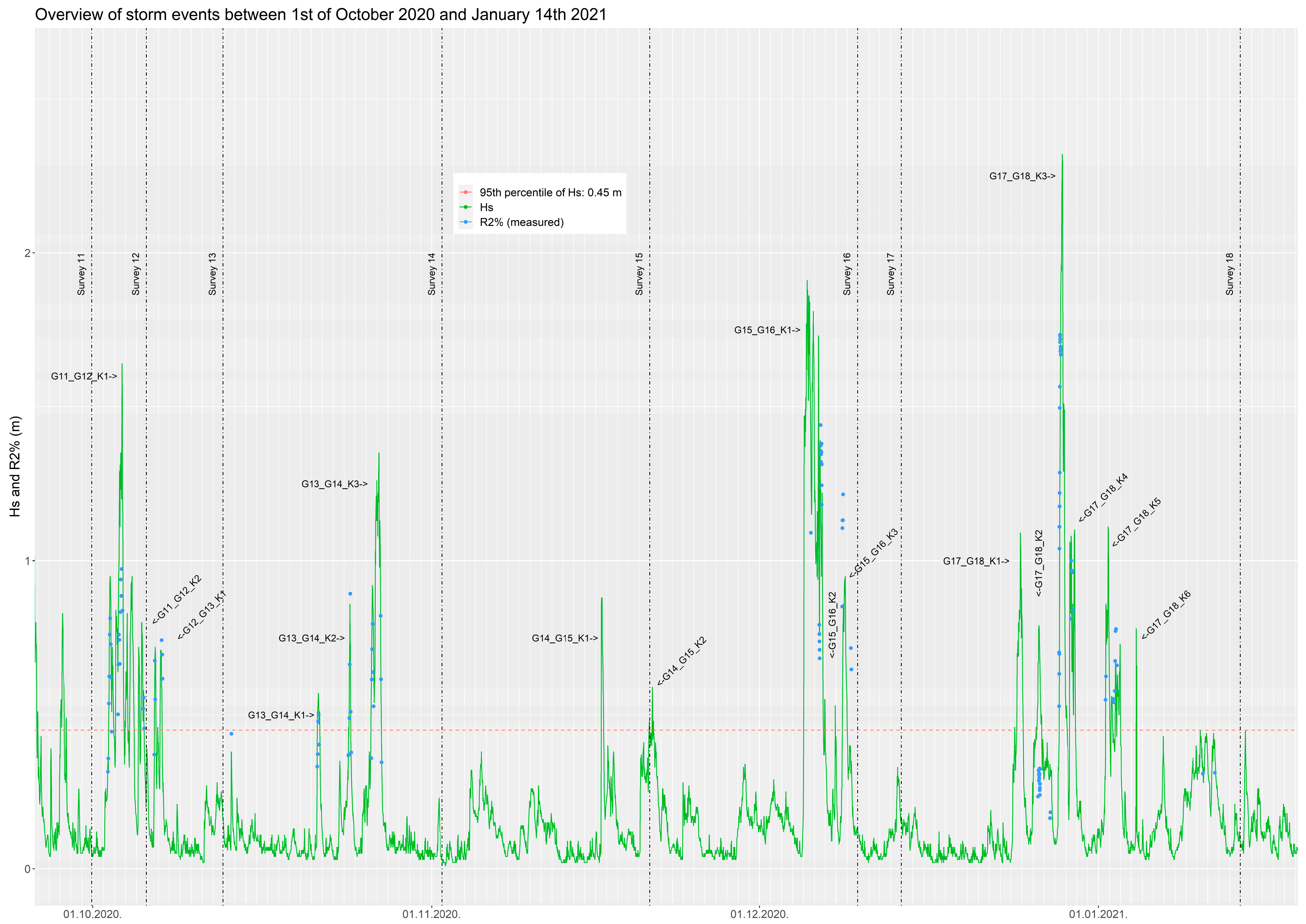
| G11 1.10.2020. | G12 6.10.2020. | K1 | 2.64 | 2.10.2020. 08:00:00 | 4.10.2020. 20:00:00 | 1.64 | 187 | Yes |
| K2 | 5.10.2020. 04:00:00 | 5.10.2020. 20:00:00 | 0.8 | 195 | Yes | |||
| G12 6.10.2020. | G13 13.10.2020. | K1 | −0.02 | 6.10.2020. 15:00:00 | 7.10.2020. 09:30:00 | 0.72 | 191 | Yes |
| G13 13.10.2020. | G14 2.11.2020. | K1 | −0.57 | 21.10.2020. 12:30:00 | 21.10.2020. 20:30:00 | 0.57 | 184 | Yes |
| K2 | 24.10.2020. 08:00:00 | 24.10.2020. 16:00:00 | 0.86 | 199 | Yes | |||
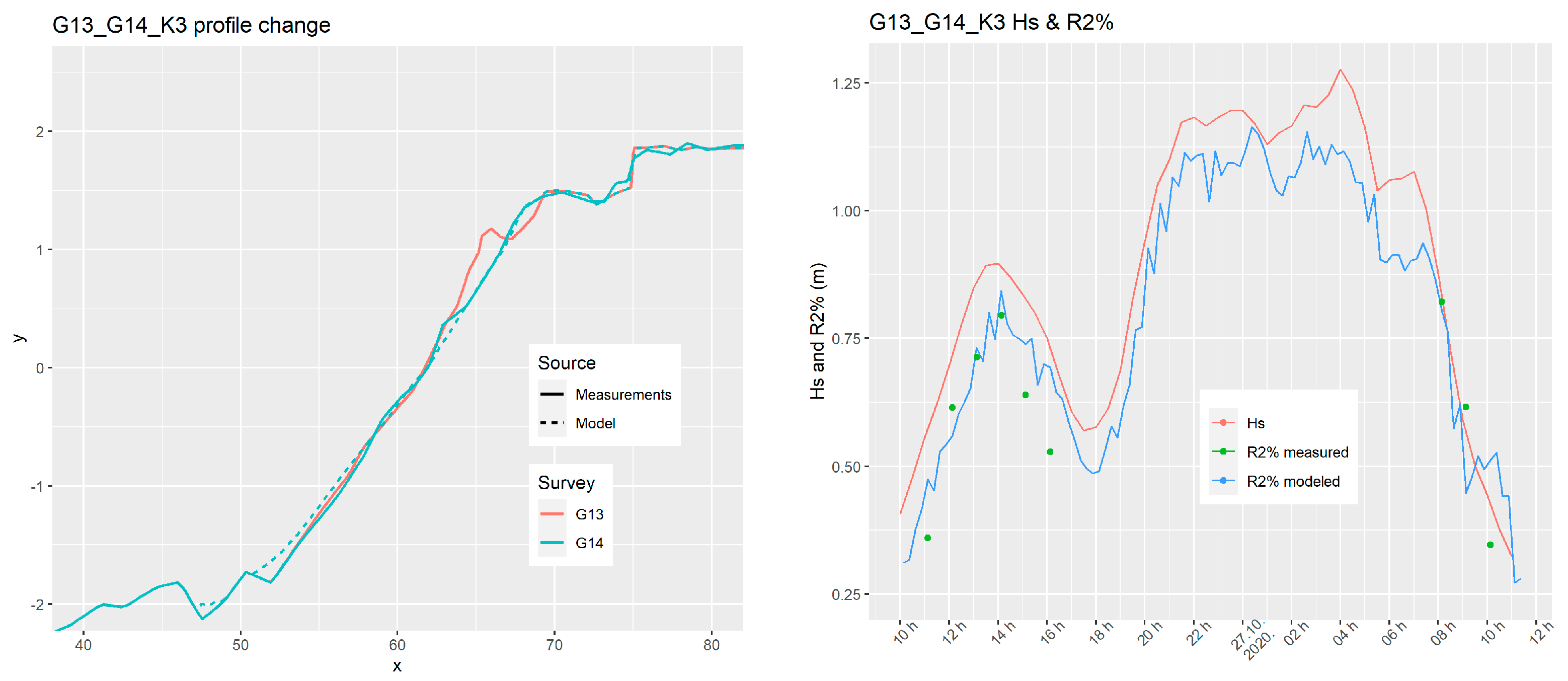
| K3 | 26.10.2020. 10:00:00 | 27.10.2020. 11:00:00 | 1.35 | 182 | Yes | |||
| G14 2.11.2020. | G15 21.11.2020. | K1 | 0.08 | 16.11.2020. 12:00:00 | 16.11.2020. 18:30:00 | 0.88 | 186 | / |
| K2 | 20.11.2020. 20:00:00 | 21.11.2020. 16:30:00 | 0.59 | 136 | / | |||
| G15 21.11.2020. | G16 10.12.2020. | K1 | 11.11 | 5.12.2020. 00:00:00 | 7.12.2020. 04:00:00 | 1.91 | 177 | Yes |
| K2 | 7.12.2020. 21:30:00 | 8.12.2020. 01:00:00 | 0.53 | 200 | / | |||
| K3 | 8.12.2020. 12:30:00 | 9.12.2020. 10:30:00 | 0.95 | 182 | Yes | |||
| G16 10.12.2020. | G17 14.12.2020. | / | −1.06 | / | ||||
| G17 14.12.2020. | G18 14.1.2021. | K1 | −5.15 | 24.12.2020. 03:00:00 | 25.12.2020. 05:00:00 | 1.09 | 199 | / |
| K2 | 26.12.2020. 04:00:00 | 27.12.2020. 17:00:00 | 0.79 | 125 | Yes | |||
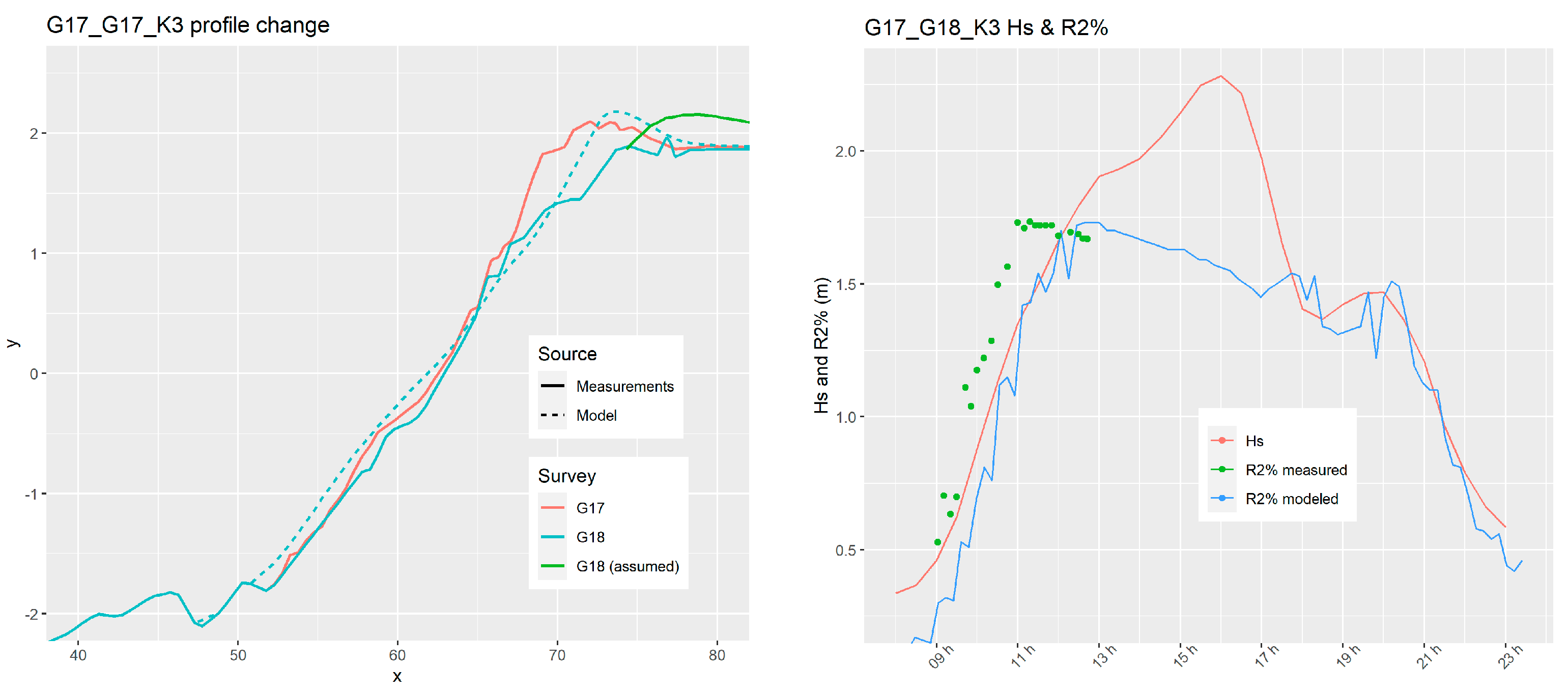
| K3 | 28.12.2020. 08:00:00 | 28.12.2020. 23:00:00 | 2.32 | 178 | Yes | |||
| K4 | 29.12.2020. 08:30:00 | 29.12.2020. 21:00:00 | 1.1 | 199 | Yes | |||
| K5 | 1.1.2021. 13:00:00 | 2.1.2021. 23:00:00 | 1.11 | 179 | Yes | |||
| K6 | 4.1.2021. 11:00:00 | 4.1.2021. 12:30:00 | 0.78 | 208 | / | |||
Appendix C

Appendix D

References
- Zadel, Z. Beaches in the Function of Primary Resource of the Beach Tourism Product. JMTS 2016, 51, 117–130. [Google Scholar] [CrossRef] [Green Version]
- Kovačić, M.; Srećko, F.; Perišić, M. The Issue of Coastal Area Management in Croatia: Beach Management. Acad. Tur. 2010, 3, 53–63. [Google Scholar]
- Hanson, H.; Brampton, A.; Capobianco, M.; Dette, H.H.; Hamm, L.; Laustrup, C.; Lechuga, A.; Spanhoff, R. Beach Nourishment Projects, Practices, and Objectives—A European Overview. Coast. Eng. 2002, 47, 81–111. [Google Scholar] [CrossRef]
- Speybroeck, J.; Bonte, D.; Courtens, W.; Gheskiere, T.; Grootaert, P.; Maelfait, J.-P.; Mathys, M.; Provoost, S.; Sabbe, K.; Stienen, E.W.M.; et al. Beach Nourishment: An Ecologically Sound Coastal Defence Alternative? A Review. Aquat. Conserv. Mar. Freshw. Ecosyst. 2006, 16, 419–435. [Google Scholar] [CrossRef]
- Pagán, J.I.; López, M.; López, I.; Tenza-Abril, A.J.; Aragonés, L. Study of the Evolution of Gravel Beaches Nourished with Sand. Sci. Total Environ. 2018, 626, 87–95. [Google Scholar] [CrossRef] [PubMed]
- Pikelj, K.; Ružić, I.; Ilić, S.; James, M.R.; Kordić, B. Implementing an Efficient Beach Erosion Monitoring System for Coastal Management in Croatia. Ocean Coast. Manag. 2018, 156, 223–238. [Google Scholar] [CrossRef] [Green Version]
- Stéphan, P.; Suanez, S.; Fichaut, B.; Autret, R.; Blaise, E.; Houron, J.; Ammann, J.; Grandjean, P. Monitoring the Medium-Term Retreat of a Gravel Spit Barrier and Management Strategies, Sillon de Talbert (North Brittany, France). Ocean Coast. Manag. 2018, 158, 64–82. [Google Scholar] [CrossRef]
- Stocker, T.F.; Qin, D.; Plattner, G.-K.; Tignor, M.M.B.; Allen, S.K.; Boschung, J.; Naules, A.; Xia, Y.; Bex, V.; Midgley, P.M. (Eds.) Climate Change 2013: The Physical Science Basis. Contribution of Working Group I to the Fifth Assessment Report of the Intergovernmental Panel on Climate Change; Cambridge University Press: Cambridge, UK; New York, NY, USA, 2014; ISBN 978-1-107-05799-9. [Google Scholar]
- Belušić Vozila, A.; Güttler, I.; Ahrens, B.; Obermann-Hellhund, A.; Telišman Prtenjak, M. Wind over the Adriatic Region in CORDEX Climate Change Scenarios. J. Geophys. Res. Atmos. 2019, 124, 110–130. [Google Scholar] [CrossRef] [Green Version]
- Belušić Vozila, A.; Telišman Prtenjak, M.; Güttler, I. A Weather-Type Classification and Its Application to Near-Surface Wind Climate Change Projections over the Adriatic Region. Atmosphere 2021, 12, 948. [Google Scholar] [CrossRef]
- Benetazzo, A.; Fedele, F.; Carniel, S.; Ricchi, A.; Bucchignani, E.; Sclavo, M. Wave Climate of the Adriatic Sea: A Future Scenario Simulation. Nat. Hazards Earth Syst. Sci. 2012, 12, 2065–2076. [Google Scholar] [CrossRef] [Green Version]
- Denamiel, C.; Pranić, P.; Quentin, F.; Mihanović, H.; Vilibić, I. Pseudo-Global Warming Projections of Extreme Wave Storms in Complex Coastal Regions: The Case of the Adriatic Sea. Clim. Dyn. 2020, 55, 2483–2509. [Google Scholar] [CrossRef]
- Bonaldo, D.; Bucchignani, E.; Pomaro, A.; Ricchi, A.; Sclavo, M.; Carniel, S. Wind Waves in the Adriatic Sea under a Severe Climate Change Scenario and Implications for the Coasts. Int. J. Climatol. 2020, 40, 5389–5406. [Google Scholar] [CrossRef]
- Međugorac, I.; Pasarić, M.; Güttler, I. Will the Wind Associated with the Adriatic Storm Surges Change in Future Climate? Appl. Clim. 2021, 143, 1–18. [Google Scholar] [CrossRef]
- Vilibić, I.; Šepić, J.; Pasarić, M.; Orlić, M. The Adriatic Sea: A Long-Standing Laboratory for Sea Level Studies. Pure Appl. Geophys. 2017, 174, 3765–3811. [Google Scholar] [CrossRef]
- Pasarić, M.; Orlić, M. Meteorological Forcing of the Adriatic: Present vs. Projected Climate Conditions. Geofizika 2004, 21, 69–87. [Google Scholar]
- Lončar, G.; Krvavica, N.; Šepić, J.; Bekić, D.; Gašparović, M.; Kulić, T. Potencijal primjene javno dostupnih baza podataka u svrhu procjene opasnosti od poplava mora u priobalnim gradovima Republike Hrvatske. Hrvat. Vode 2022, 30, 185–200. [Google Scholar]
- Vousdoukas, M.I.; Voukouvalas, E.; Annunziato, A.; Giardino, A.; Feyen, L. Projections of Extreme Storm Surge Levels along Europe. Clim. Dyn. 2016, 47, 3171–3190. [Google Scholar] [CrossRef] [Green Version]
- Bujak, D.; Bogovac, T.; Carević, D.; Ilic, S.; Lončar, G. Application of Artificial Neural Networks to Predict Beach Nourishment Volume Requirements. JMSE 2021, 9, 786. [Google Scholar] [CrossRef]
- McCall, R.T.; Masselink, G.; Poate, T.G.; Roelvink, J.A.; Almeida, L.P. Modelling the Morphodynamics of Gravel Beaches during Storms with XBeach-G. Coast. Eng. 2015, 103, 52–66. [Google Scholar] [CrossRef]
- McCall, R.T.; Masselink, G.; Poate, T.G.; Roelvink, J.A.; Almeida, L.P.; Davidson, M.; Russell, P.E. Modelling Storm Hydrodynamics on Gravel Beaches with XBeach-G. Coast. Eng. 2014, 91, 231–250. [Google Scholar] [CrossRef] [Green Version]
- Almeida, L.P.; Masselink, G.; McCall, R.; Russell, P. Storm Overwash of a Gravel Barrier: Field Measurements and XBeach-G Modelling. Coast. Eng. 2017, 120, 22–35. [Google Scholar] [CrossRef] [Green Version]
- Ions, K.; Karunarathna, H.; Reeve, D.E.; Pender, D. Gravel Barrier Beach Morphodynamic Response to Extreme Conditions. JMSE 2021, 9, 135. [Google Scholar] [CrossRef]
- Poate, T.G.; McCall, R.T.; Masselink, G. A New Parameterisation for Runup on Gravel Beaches. Coast. Eng. 2016, 117, 176–190. [Google Scholar] [CrossRef] [Green Version]
- Bergillos, R.J.; Masselink, G.; Ortega-Sánchez, M. Coupling Cross-Shore and Longshore Sediment Transport to Model Storm Response along a Mixed Sand-Gravel Coast under Varying Wave Directions. Coast. Eng. 2017, 129, 93–104. [Google Scholar] [CrossRef] [Green Version]
- Brown, S.I.; Dickson, M.E.; Kench, P.S.; Bergillos, R.J. Modelling Gravel Barrier Response to Storms and Sudden Relative Sea-Level Change Using XBeach-G. Mar. Geol. 2019, 410, 164–175. [Google Scholar] [CrossRef]
- Grottoli, E.; Bertoni, D.; Ciavola, P. Short- and Medium-Term Response to Storms on Three Mediterranean Coarse-Grained Beaches. Geomorphology 2017, 295, 738–748. [Google Scholar] [CrossRef]
- Williams, J.J.; Buscombe, D.; Masselink, G.; Turner, I.L.; Swinkels, C. Barrier Dynamics Experiment (BARDEX): Aims, Design and Procedures. Coast. Eng. 2012, 63, 3–12. [Google Scholar] [CrossRef]
- López de San Román-Blanco, B.; Coates, T.T.; Holmes, P.; Chadwick, A.J.; Bradbury, A.; Baldock, T.E.; Pedrozo-Acuña, A.; Lawrence, J.; Grüne, J. Large Scale Experiments on Gravel and Mixed Beaches: Experimental Procedure, Data Documentation and Initial Results. Coast. Eng. 2006, 53, 349–362. [Google Scholar] [CrossRef]
- Lončar, G.; Carević, D.; Ilić, S.; Krvavica, N.; Kalinić, F. Morfodinamika šljunčanog žala Ploče u uvjetima jakog juga. Hrvat. Vode 2020, 28, 205–216. [Google Scholar]
- Lončar, G.; Kalinić, F.; Carević, D.; Bujak, D. Numerical Modelling of the Morphodynamics of the Ploče Gravel Beach in Rijeka. e-GFOS 2021, 12, 33–48. [Google Scholar] [CrossRef]
- Tadić, A.; Ružić, I.; Krvavica, N.; Ilić, S. Post-Nourishment Changes of an Artificial Gravel Pocket Beach Using UAV Imagery. JMSE 2022, 10, 358. [Google Scholar] [CrossRef]
- Holman, R.A.; Stanley, J. The History and Technical Capabilities of Argus. Coast. Eng. 2007, 54, 477–491. [Google Scholar] [CrossRef]
- Bujak, D.; Ilic, S.; Miličević, H.; Carević, D. Wave Runup Prediction and Alongshore Variability on a Pocket Gravel Beach under Fetch-Limited Wave Conditions. J. Mar. Sci. Eng. 2023, 11, 614. [Google Scholar] [CrossRef]
- Powell, K.A. Predicting Short Term Profile Response for Shingle Beaches; Hydraulics Research Wallingford: Wallingford, UK, 1990. [Google Scholar]
- Roelvink, D.; Reniers, A.; van Dongeren, A.; van Thiel de Vries, J.; McCall, R.; Lescinski, J. Modelling Storm Impacts on Beaches, Dunes and Barrier Islands. Coast. Eng. 2009, 56, 1133–1152. [Google Scholar] [CrossRef]
- van Rijn, L.C.; Walstra, D.J.R.; Grasmeijer, B.; Sutherland, J.; Pan, S.; Sierra, J.P. The Predictability of Cross-Shore Bed Evolution of Sandy Beaches at the Time Scale of Storms and Seasons Using Process-Based Profile Models. Coast. Eng. 2003, 47, 295–327. [Google Scholar] [CrossRef]
- Hazen, A. Some Physical Properties of Sands and Gravels, with Special Reference to Their Use in Filtration. In Volume II State Sanitation: A Review of the Work of the Massachusetts State Board of Health, Volume II; Harvard University Press: Cambridge, MA, USA, 2013; pp. 232–248. ISBN 978-0-674-60048-5. [Google Scholar]
- Engstrom, W. A Method of Predicting Beach Orientation. Prof. Geogr. 1973, 25, 12–15. [Google Scholar] [CrossRef]


| Test 1 | Test 2 | Test 3 | |
|---|---|---|---|
| Hs (m) | 0.6 | 1 | 1.2 |
| Tp (s) | 3.22 | 4.14 | 4.48 |
| Duration (s) | 8400 | 7200 | 7800 |
| Steepness | 0.05 | ||
| Brier Skill Score | Qualification |
|---|---|
| 0.8–1 | Excellent |
| 0.6–0.8 | Good |
| 0.3–0.6 | Fair |
| 0–0.3 | Poor |
| <0 | Bad |
Disclaimer/Publisher’s Note: The statements, opinions and data contained in all publications are solely those of the individual author(s) and contributor(s) and not of MDPI and/or the editor(s). MDPI and/or the editor(s) disclaim responsibility for any injury to people or property resulting from any ideas, methods, instructions or products referred to in the content. |
© 2023 by the authors. Licensee MDPI, Basel, Switzerland. This article is an open access article distributed under the terms and conditions of the Creative Commons Attribution (CC BY) license (https://creativecommons.org/licenses/by/4.0/).
Share and Cite
Bogovac, T.; Carević, D.; Bujak, D.; Miličević, H. Application of the XBeach-Gravel Model for the Case of East Adriatic Sea-Wave Conditions. J. Mar. Sci. Eng. 2023, 11, 680. https://doi.org/10.3390/jmse11030680
Bogovac T, Carević D, Bujak D, Miličević H. Application of the XBeach-Gravel Model for the Case of East Adriatic Sea-Wave Conditions. Journal of Marine Science and Engineering. 2023; 11(3):680. https://doi.org/10.3390/jmse11030680
Chicago/Turabian StyleBogovac, Tonko, Dalibor Carević, Damjan Bujak, and Hanna Miličević. 2023. "Application of the XBeach-Gravel Model for the Case of East Adriatic Sea-Wave Conditions" Journal of Marine Science and Engineering 11, no. 3: 680. https://doi.org/10.3390/jmse11030680